5G-NR
5G New Radio
3GPP
3rd Generation Partnership Project
AC
address coding
ACF
autocorrelation function
ACR
autocorrelation receiver
ADC
analog-to-digital converter
AIC
Analog-to-Information Converter
AIC
Akaike information criterion
ARIC
asymmetric restricted isometry constant
ARIP
asymmetric restricted isometry property
CF
closed form
IM/DD
intensity modulation direct detection
ARQ
automatic repeat request
AUB
asymptotic union bound
AWGN
Additive White Gaussian Noise
S-I
signal-independent
CFA
closed-form (CF) algorithm
AWGN
additive white Gaussian noise
CRB
Cramér-Rao bound
BCRB
Bayesian CRB
BA
Blahut–Arimoto
BAA
Blahut–Arimoto Algorithm
ISAC
integrated sensing and communication
AR-D
achievable rate-distortion
AR-CRB
achievable rate- Cramér-Rao bound (CRB)
C-D
capacity-distortion
EC-D
enhanced capacity-distortion
R-D
rate-distortion
TS
time sharing
PSK
asymmetric PSK
SRC
sensing response channel
CC
communication channel
AoD
angle of departure
AoA
angle of arrival
AWRICs
asymmetric weak restricted isometry constants
AWRIP
asymmetric weak restricted isometry property
BCH
Bose, Chaudhuri, and Hocquenghem
BCHSC
BCH based source coding
BEP
bit error probability
BFC
block fading channel
BG
Bernoulli-Gaussian
BGG
Bernoulli-Generalized Gaussian
BPAM
binary pulse amplitude modulation
BPDN
Basis Pursuit Denoising
BPPM
binary pulse position modulation
BPSK
binary phase shift keying
BPZF
bandpass zonal filter
BSC
binary symmetric channels
BU
Bernoulli-uniform
BER
bit error rate
BS
base station
LS
least squares
SISO-COM and SIMO-SEN
single-input single-output for communication and single-input multiple output for sensing
CP
Cyclic Prefix
CDF
cumulative distribution function
CDF
cumulative distribution function
CDF
cumulative distribution function
CCDF
complementary cumulative distribution function
CCDF
complementary CDF
CCDF
complementary cumulative distribution function
CD
cooperative diversity
MAP
maximum a posteriori
CDMA
Code Division Multiple Access
ch.f.
characteristic function
CIR
channel impulse response
CoSaMP
compressive sampling matching pursuit
CR
cognitive radio
CS
compressed sensing
CS
Compressed sensing
CS
compressed sensing
CSI
channel state information
CCSDS
consultative committee for space data systems
COVID-19
Coronavirus disease
IB
inner bound
DAA
detect and avoid
DAB
digital audio broadcasting
DCT
discrete cosine transform
DFT
discrete Fourier transform
DR
distortion-rate
DS
direct sequence
DS-SS
direct-sequence spread-spectrum
DTR
differential transmitted-reference
DVB-H
digital video broadcasting – handheld
DVB-T
digital video broadcasting – terrestrial
DL
downlink
DSSS
Direct Sequence Spread Spectrum
DFT-s-OFDM
Discrete Fourier Transform-spread-Orthogonal Frequency Division Multiplexing
DAS
distributed antenna system
DNA
Deoxyribonucleic Acid
EC
European Commission
EED
exact eigenvalues distribution
EIRP
Equivalent Isotropically Radiated Power
ELP
equivalent low-pass
eMBB
Enhanced Mobile Broadband
EMF
electric and magnetic fields
EU
European union
FC
fusion center
FCC
Federal Communications Commission
FEC
forward error correction
FFT
fast Fourier transform
FH
frequency-hopping
FH-SS
frequency-hopping spread-spectrum
FS
Frame synchronization
FS
frame synchronization
FDMA
Frequency Division Multiple Access
GA
Gaussian approximation
GF
Galois field
GG
Generalized-Gaussian
GIC
generalized information criterion
GLRT
generalized likelihood ratio test
GPS
Global Positioning System
GMSK
Gaussian minimum shift keying
GSMA
Global System for Mobile communications Association
HAP
high altitude platform
IDR
information distortion-rate
IFFT
inverse fast Fourier transform
IHT
iterative hard thresholding
i.i.d.
independent, identically distributed
IoT
Internet of Things
IR
impulse radio
LRIC
lower restricted isometry constant
LRICt
lower restricted isometry constant threshold
ISI
intersymbol interference
ITU
International Telecommunication Union
ICNIRP
International Commission on Non-Ionizing Radiation Protection
IEEE
Institute of Electrical and Electronics Engineers
ICES
IEEE international committee on electromagnetic safety
IEC
International Electrotechnical Commission
IARC
International Agency on Research on Cancer
IS-95
Interim Standard 95
KKT
Karush–Kuhn–Tucker
LEO
low earth orbit
LF
likelihood function
LLF
log-likelihood function
LLR
log-likelihood ratio
LLRT
log-likelihood ratio test
LoS
line-of-sight
LRT
likelihood ratio test
LWRIC
lower weak restricted isometry constant
LWRICt
LWRIC threshold
LPWAN
low power wide area network
LoRaWAN
Low power long Range Wide Area Network
NLOS
non-line-of-sight
MB
multiband
MC
multicarrier
MDS
mixed distributed source
MF
matched filter
m.g.f.
moment generating function
MI
mutual information
MIMO
multiple-input multiple-output
MISO
multiple-input single-output
MJSO
maximum joint support cardinality
ML
machine learning
MLE
maximum likelihood estimator
GD
gradient descent
MMSE
minimum mean-square error
LMMSE
linear minimum mean-square error
MSE
mean-square error
MMV
multiple measurement vectors
MOS
model order selection
${M}$-PSK
$M$-ary phase shift keying
${M}$-PSK
$M$-ary asymmetric PSK
$M$-QAM
$M$-ary quadrature amplitude modulation
MRC
maximal ratio combiner
MSO
maximum sparsity order
M2M
machine to machine
MUI
multi-user interference
mMTC
massive Machine Type Communications
mm-Wave
millimeter-wave
MP
mean posterior
MPE
maximum permissible exposure
MAC
media access control
NB
narrowband
NBI
narrowband interference
NLA
nonlinear sparse approximation
NLOS
Non-Line of Sight
NTIA
National Telecommunications and Information Administration
NTP
National Toxicology Program
NHS
National Health Service
OC
optimum combining
OC
optimum combining
ODE
operational distortion-energy
ODR
operational distortion-rate
OFDM
orthogonal frequency-division multiplexing
OMP
orthogonal matching pursuit
OSMP
orthogonal subspace matching pursuit
OQAM
offset quadrature amplitude modulation
OQPSK
offset QPSK
OFDMA
Orthogonal Frequency-division Multiple Access
OPEX
Operating Expenditures
OQPSK/PM
OQPSK with phase modulation
PAM
pulse amplitude modulation
PAR
peak-to-average ratio
PDF
probability density function
PDF
probability density function
PDF
probability distribution function
PDP
power dispersion profile
PMF
probability mass function
ROST
Repetition-One Shot Trade-Off
PMF
probability mass function
PN
pseudo-noise
PPM
pulse position modulation
PRake
Partial Rake
PSD
power spectral density
PSEP
pairwise synchronization error probability
PSK
phase shift keying
PD
power density
$8$-PSK
$8$-phase shift keying
RCS
radar cross section
AR-D-GT
Achievable Rate-Distortion-Ground Truth
FSK
frequency shift keying
CVAE
Conditional Variational Auto-encoder
FIM
Fisher information matrix
QAM
Quadrature Amplitude Modulation
QPSK
quadrature phase shift keying
OQPSK/PM
OQPSK with phase modulator
RD
raw data
RDL
"random data limit"
RIC
restricted isometry constant
RICt
restricted isometry constant threshold
RIP
restricted isometry property
ROC
receiver operating characteristic
RQ
Raleigh quotient
RS
Reed-Solomon
RSSC
RS based source coding
r.v.
random variable
R.V.
random vector
RMS
root mean square
RFR
radiofrequency radiation
RIS
Reconfigurable Intelligent Surface
RNA
RiboNucleic Acid
SA-Music
subspace-augmented MUSIC with OSMP
SCBSES
Source Compression Based Syndrome Encoding Scheme
SCM
sample covariance matrix
SEP
symbol error probability
SG
sparse-land Gaussian model
SIMO
single-input multiple-output
SINR
signal-to-interference plus noise ratio
SIR
signal-to-interference ratio
SISO
single-input single-output
SMV
single measurement vector
SNR
signal-to-noise ratio
O-SNR
optical signal-to-noise ratio
SP
subspace pursuit
SS
spread spectrum
SW
sync word
SAR
specific absorption rate
SSB
synchronization signal block
TH
time-hopping
ToA
time-of-arrival
TR
transmitted-reference
TW
Tracy-Widom
TWDT
TW Distribution Tail
TCM
trellis coded modulation
TDD
time-division duplexing
TDMA
time division multiple access
DRT
deterministic-random tradeoff
UAV
unmanned aerial vehicle
URIC
upper restricted isometry constant
URICt
upper restricted isometry constant threshold
S&C
sensing and communication
O-ISAC
optical ISAC
UWB
ultrawide band
UWB
Ultrawide band
URLLC
Ultra Reliable Low Latency Communications
FOV
field of view
UWRIC
upper weak restricted isometry constant
UWRICt
UWRIC threshold
UE
user equipment
UL
uplink
ULA
uniform linear array
P2P
point-to-point
SDMC-DF
state-dependent memoryless channel with delayed feedback
Comm. Rx
communication receiver
Tx
transmitter
Sens. Rx
sensing receiver
WiM
weigh-in-motion
WLAN
wireless local area network
WM
Wishart matrix
WMAN
wireless metropolitan area network
WPAN
wireless personal area network
WRIC
weak restricted isometry constant
WRICt
weak restricted isometry constant thresholds
WRIP
weak restricted isometry property
WSN
wireless sensor network
WSS
wide-sense stationary
WHO
World Health Organization
Wi-Fi
wireless fidelity
CF
closed-form
SpaSoSEnc
sparse source syndrome encoding
OB
outer bound
UB
upper bound
LB
lower bound
CLT
central limit theorem
LiSAC
Lighting, Sensing, and Communication
VLC
visible light communication
VPN
virtual private network
RF
radio frequency
FSO
free space optical
IoST
Internet of space things
Comm. Opt.
communication optimal
Sens. Opt.
sensing optimal
w.r.t.
with respect to
LiDAR
Light Detection and Ranging
GSM
Global System for Mobile Communications
2G
second-generation cellular network
3G
third-generation cellular network
4G
fourth-generation cellular network
5G
5th-generation cellular network
gNB
next generation node B base station
NR
New Radio
UMTS
Universal Mobile Telecommunications Service
LTE
Long Term Evolution
QoS
quality of service

Optical ISAC: Fundamental Performance Limits and Transceiver Design

Alireza Ghazavi Khorasgani, Mahtab Mirmohseni, Ahmed Elzanaty 0009-0001-9141-7260 0000-0002-5247-5820 0000-0001-8854-8369 5/6GIC, Institute for Communication Systems (ICS), University of Surrey, Guildford, United Kingdom
{a.ghazavi, m.mirmohseni, a.elzanaty}@surrey.ac.uk
Abstract

This paper characterizes the optimal capacity-distortion (C-D) tradeoff in an optical point-to-point (P2P) system with single-input single-output for communication and single-input multiple-output for sensing (SISO-COM and SIMO-SEN) within an integrated sensing and communication (ISAC) framework. We consider the optimal rate-distortion (R-D) region and explore several inner (IB) and outer (OB) bounds. We introduce practical, asymptotically optimal maximum a posteriori (MAP) and maximum likelihood estimators (MLE) for target distance, addressing nonlinear measurement-to-state relationships and non-conjugate priors. As the number of sensing antennas increases, these estimators converge to the Bayesian Cramér-Rao bound (BCRB). We also establish that the achievable rate-CRB (AR-CRB) serves as an OB for the optimal C-D region, valid for both unbiased estimators and asymptotically large numbers of receive antennas. To clarify that the input distribution determines the tradeoff across the Pareto boundary of the C-D region, we propose two algorithms: i) an iterative Blahut-Arimoto algorithm (BAA)-type method, and ii) a memory-efficient closed-form (CF) approach. The CF approach includes a CF optimal distribution for high optical signal-to-noise ratio (O-SNR) conditions. Additionally, we adapt and refine the Deterministic-Random Tradeoff (DRT) to this optical ISAC context.

Index Terms:
Optical Integrated Sensing and Communication (O-ISAC), Bayesian Cramér-Rao Bound (BCRB), optimal input distribution, modified Deterministic-Random Tradeoff (DRT)

I Introduction

Future wireless networks aim to integrate advanced sensing with communication, essential for applications like intelligent transportation and smart cities. \AcISAC systems epitomize this convergence, sharing hardware, spectrum, and signaling for both sensing and communication (S&C) [1, 2]. While radio frequency (RF) integrated sensing and communication (ISAC) has been the primary focus, optical ISAC (O-ISAC) is emerging as a promising complement, particularly in free space optical (FSO) systems, which offer unique advantages in optical communication and sensing [3].

Previous works consider RF ISAC system [4, 5, 6, 7, 8, 9]. In [4], the optimal capacity-distortion (C-D) for single-antenna RF ISAC systems was explored. The optimal estimator simplifies to the linear minimum mean-square error (LMMSE) estimator under specific conditions (i.e., Gaussian priors), but real-world scenarios often involve nonlinear functions of sensing response channel (SRC) and non-conjugate priors, such as estimating distance from an echo signal, which complicates the computation of the optimal estimator [10]. Significant research has addressed the achievable rate- (AR-CRB) tradeoff in single-input single-output for communication and single-input multiple output for sensing (SISO-COM and SIMO-SEN) RF channels, particularly for parameters like angle of departure (AoD) and angle of arrival (AoA) [5, 6, 9, 7]. However, gaps remain in practical estimators, transceiver design, and optimal C-D regions. Additionally, most studies have focused on Gaussian signaling, which may not fully exploit the potential benefits for ISAC. To enhance observations, one solution is to record multiple feedbacks across several channel uses with block-wise independent, identically distributed (i.i.d.) states (block length $T$). While this improves sensing performance, it degrades communication performance proportionally to $T^{-1}$, especially for large $T$ [5, Eq. 36]. While all existing works focus on RF signals, which differ significantly from optical systems due to the positive and real nature of the signals, to the best of our knowledge, O-ISAC systems have not been explored in terms of information-theoretical fundamental limits.

This paper makes several key contributions: i) We characterize the optimal Pareto boundary of the achievable rate-distortion (AR-D) and C-D regions for an optical point-to-point (P2P) SISO-COM and SIMO-SEN ISAC system, which leverages multiple antennas to enhance both communication and sensing, focusing particularly on target distance estimation with nonlinear SRC relationships and non-conjugate priors. ii) We adapt and refine the deterministic-random tradeoff (DRT) [5] for optical SISO-COM and SIMO-SEN ISAC and general estimators, introducing practical, asymptotically optimal estimators. We analyze the performance of our proposed maximum a posteriori (MAP) and maximum likelihood estimator (MLE) estimators, demonstrating their convergence to the CRB as the number of sensing antennas increases. iii) We demonstrate that, in asymptotic scenarios, the AR-CRB serves as an outer bound (OB), while the MAP, MLE, and any unbiased estimator function as an inner bound (IB) for the optimal C-D region. iv) We propose two algorithms to determine the optimal input distribution for the Pareto boundary of the C-D region, validate these algorithms against the endpoints, and characterize the optimal O-ISAC input distribution under high optical signal-to-noise ratio (O-SNR) regime ($\textrm{\acs{O-SNR}}\triangleq\frac{\mathbb{E}[X]}{\sigma_{\textrm{c}}^{2}}\gg 1$).

Notation: Sets are denoted by calligraphic letters (e.g., $\mathcal{X}$), with cardinality $\lvert\mathcal{X}\rvert$. Real numbers are $\mathbb{R}$; nonnegative reals are $\mathbb{R}_{0}^{+}$. Random variables are uppercase (e.g., $X$), and realizations are lowercase (e.g., $x$). Vectors are boldfaced (e.g., $\boldsymbol{Y}_{\textrm{s}}$). Key symbols include $\sim$ (distribution), $\perp\!\!\!\perp$ (independence), and $\overset{a}{\sim}$ (asymptotic distribution). Functions/operators: $\mathcal{N}(\mu,\sigma^{2})$ (Gaussian), $\mathcal{H}(\cdot)$ (entropy), $\mathcal{I}(\cdot)$ ( mutual information (MI)), $\mathbb{E}_{X}[\cdot]$ (expectation), $|\cdot|$ (absolute value), and $\|\cdot\|$ ($\ell_{2}$ norm).

II System Model

Refer to caption
Fig. 1: O-ISAC system with memoryless channels.

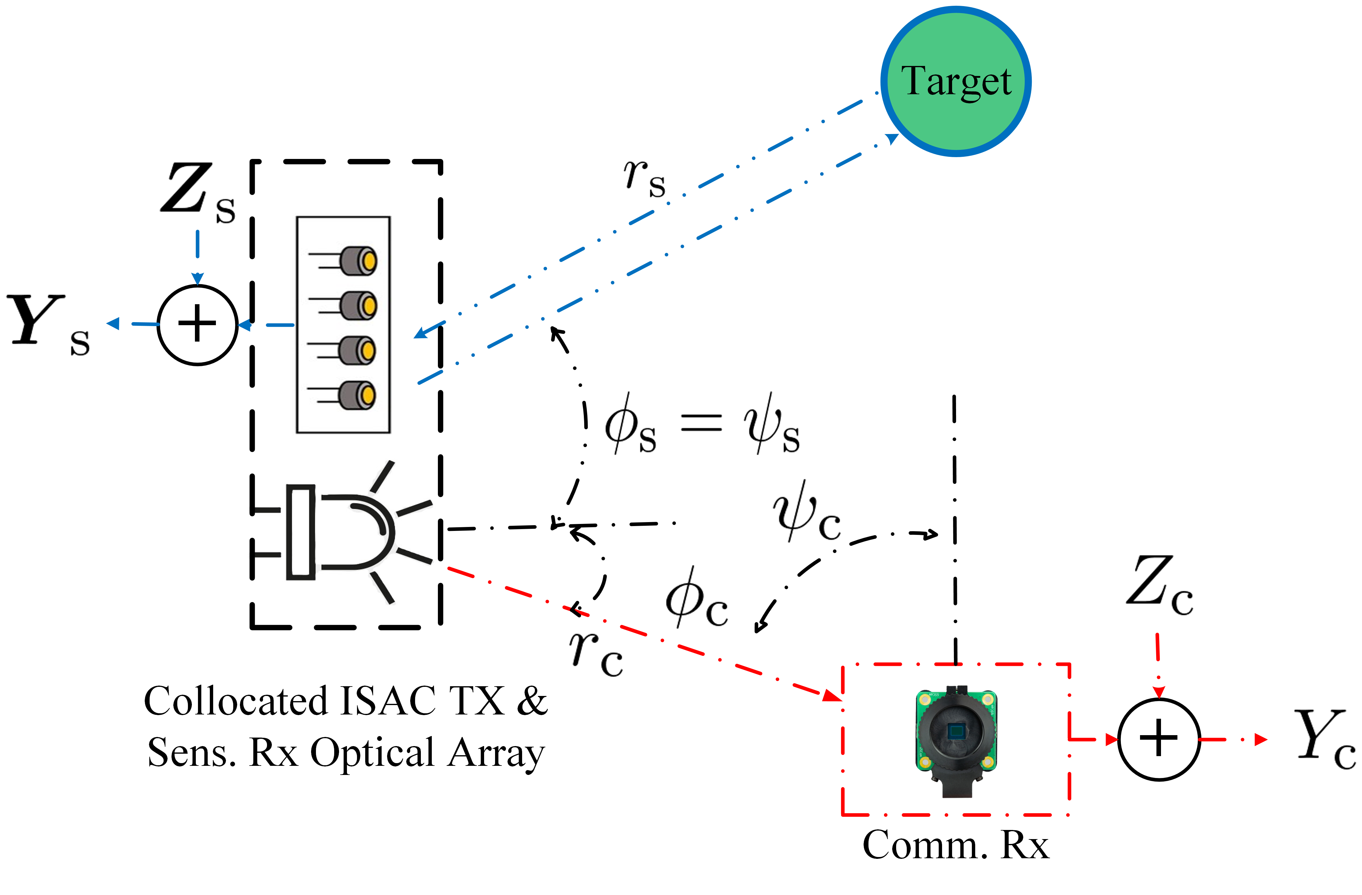
We consider a P2P O-ISAC system, as illustrated in Fig.​ 1. This system comprises a single-antenna transmitter (Tx), an $n_{\textrm{s}}$-antenna monostatic sensing receiver (Sens. Rx) that is collocated with the Tx, a single-antenna communication receiver (Comm. Rx), and a point-wise target. This configuration is typical for Light Detection and Ranging (LiDAR) evaluations [11]. In this setup, data is transmitted to the Comm. Rx while simultaneously estimating the target distance $R_{\textrm{s}}\in\mathbb{R}_{0}^{+}$, with the realization denoted as $r_{\textrm{s}}$. The distance estimation is based on echoes received at the Sens. Rx. Additionally, we use a state-dependent FSO ISAC channel with intensity modulation direct detection (IM/DD), which is detected by both receivers [12, 13].

Communication and Sensing Models: The received signal at Comm. Rx during the $i$-th channel use is:

$$Y_{\textrm{c},i}=h_{\textrm{c}}X_{i}+Z_{\textrm{c},i},$$ (1)

where $h_{\textrm{c}}\in\mathbb{R}$ is the line-of-sight (LoS) communication channel (CC), $X_{i}$ is the transmitted signal, and $Z_{\textrm{c},i}\sim\mathcal{N}(0,\sigma_{\textrm{c}}^{2})$ is i.i.d. additive white Gaussian noise (AWGN). The CC is:

$$h_{\textrm{c}}=\frac{A}{r_{\textrm{c}}^{2}}R_{\textrm{0}}(\phi_{\textrm{c}})T_{\textrm{s}}(\psi_{\textrm{c}})g(\psi_{\textrm{c}})\cos{\psi_{\textrm{c}}}\cdot\mathbf{1}_{[0,\textrm{FOV}]}(\psi_{\textrm{c}}),$$ (2)

where $r_{\textrm{c}}$ is the distance between Tx and Comm. Rx, $\phi_{\textrm{c}}$ and $\psi_{\textrm{c}}$ are angles relative to Tx and Comm. Rx, $T_{\textrm{s}}(\cdot)$ is the concentrator gain, $A$ is the effective area, and FOV is the field of view (FOV). The Tx radiant intensity gain is $R_{\textrm{0}}(\phi)=\frac{(m+1)}{2\pi}\cos^{m}{\phi}$, where $m=-\frac{\ln{2}}{\ln{(\cos{\Phi_{1/2}})}}$ [12].

The echo signal received at Sens. Rx at the $i$-th channel use is:

$$\boldsymbol{Y}_{\textrm{s},i}=\boldsymbol{h}_{\textrm{s}}(R_{\textrm{s},i})X_{i}+\boldsymbol{Z}_{\textrm{s},i},$$ (3)

where $\boldsymbol{h}_{\textrm{s}}(R_{\textrm{s},i})\in\mathbb{R}^{n_{\textrm{s}}\times 1}$ is the target response coefficient dependent on $R_{\textrm{s},i}$, and $\boldsymbol{Z}_{\textrm{s},i}\sim\mathcal{N}(0,\sigma_{\text{S}}^{2}\boldsymbol{I}_{n_{\textrm{s}}})$. The target response matrix $h_{\textrm{s},j,i}(r_{\textrm{s},j,i})$ is:

$$h_{\textrm{s},j,i}(r_{\textrm{s},j,i})=\frac{\textrm{RCS}}{r_{\textrm{s},j,i}^{4}}R_{\text{0}}(0)T_{\text{s}}(\psi_{\textrm{s}})g(\psi_{\textrm{s}})\cos{\psi_{\textrm{s}}}\cdot\mathbf{1}_{[0,\textrm{FOV}]}(\phi_{\textrm{s}}),$$ (4)

where $\textrm{RCS}=A^{2}R_{\text{0}}(\phi_{\textrm{s}})T_{\text{s}}(0)g(0)R_{\text{0}}(0)T_{\text{s}}(\psi_{\textrm{s}})g(\psi_{\textrm{s}})\cos{\phi_{\textrm{s}}}$ is the radar cross section (RCS), assuming perfect RCS and no additional noise from reflection [14]. With Sens. Rx antennas arranged in a uniform linear array (ULA) and the target moving along a straight line, $\psi_{\textrm{s}}$ and $\psi_{\textrm{c}}$ remain constant. Assuming $r_{\textrm{s}}\gg\Delta r_{\textrm{s}}$, we have $r_{\textrm{s},j,i}\approx r_{\textrm{s},i}$ for all $i,j$.111A uniform $8\times 8$ array with $11.2\,\mu\text{m}$ spacing ensures a FOV of $8^{\circ}$. 222Phase shifts are immeasurable in IM/DD [12]. [15].

Code Definition: A $(2^{nR},n)$ code for state-dependent memoryless channel with delayed feedback (SDMC-DF) includes several components. First, there is a discrete message set $M$ with $\lvert M\rvert=2^{nR}$. Second, encoding functions $\phi_{i}:\mathcal{M}\times\mathcal{Y}_{\textrm{s}}^{i-1}\mapsto\mathcal{X}$ are defined for $i=1,2,\dots,n$. Third, a decoding function $f:\mathcal{R}_{\textrm{s}}^{n}\times\mathcal{Y}_{c}^{n}\mapsto\mathcal{M}$ is provided. Fourth, a state estimator $h:\mathcal{X}\times\mathcal{Y}_{\textrm{s}}^{n}\mapsto\hat{R_{\textrm{s}}}^{n}$ is included, with $\hat{R_{\textrm{s}}}$ as the reconstruction alphabet. For a given code, the random message $M$ is uniformly distributed over $\mathcal{M}$. Inputs are generated as $X_{i}=\varphi_{i}(W,\boldsymbol{Y}_{\textrm{s}}^{i-1})$ for $i=1,\dots,n$. The channel outputs $Y_{\textrm{c},i}$ and $\boldsymbol{Y}_{\textrm{s},i}$ at time $i$ depend on the state $R_{\textrm{s},i}$ and the input $X_{i}$. These dependencies are governed by the transition laws $P_{Y_{\textrm{c}}\mid X,R_{\textrm{s}}}(\cdot\mid x_{i},r_{\textrm{s},i})$ and $P_{\boldsymbol{Y}_{\textrm{s}}\mid X,R_{\textrm{s}}}(\cdot\mid x_{i},r_{\textrm{s},i})$, as given in (3) and (1). Let $\hat{R_{\textrm{s}}}^{n}\triangleq(\hat{R_{\textrm{s}}}_{s,1},\dots,\hat{R_{\textrm{s}}}_{s,n})=h(X^{n},Y_{\textrm{c}}^{n})$ denote state estimate at Tx, and $\hat{W}=g(R_{\textrm{s}}^{n},Y_{\textrm{c}}^{n})$ the decoded message at Comm. Rx. The quality of state estimation is measured by the expected average per-block distortion: $\Delta^{(n)}\triangleq\mathbb{E}[d(R_{\textrm{s}}^{n},\hat{R_{\textrm{s}}}^{n})]=\frac{1}{n}\sum_{i=1}^{n}\mathbb{E}[d(R_{\textrm{s},i},\hat{R_{\textrm{s}}}_{s,i})]$, where $d:\mathcal{R}_{\textrm{s}}\times\hat{R_{\textrm{s}}}\to\mathbb{R}_{0}^{+}$ is a bounded distortion function with $\max_{(r_{\textrm{s}},\hat{r_{\textrm{s}}})\in\mathcal{R}_{\textrm{s}}\times\hat{\mathcal{R}}_{s}}d(r_{\textrm{s}},\hat{r_{\textrm{s}}})<\infty$. In practical optical systems, $X$ is proportional to optical intensity and thus nonnegative: $X\in\mathbb{R}_{0}^{+}$. Then, $\mathbb{E}[|X^{n}|]=\frac{1}{n}\sum_{i=1}^{n}\mathbb{E}[|X_{i}|]$333The monostatic Sens. Rx, collocated with Tx, knows $X^{n}$ [5]. It estimates $R_{\textrm{s}}$ from $\boldsymbol{Y}_{\textrm{s}}^{n}$, while Comm. Rx decodes $M$ from $Y_{\textrm{c}}^{n}$..

Definition 1.

(C-D Region) A C-D tuple $(C,D)$ is achievable with power budget $P$ if there exists a sequence of $(2^{nR},n)$ codes that satisfies:

$\displaystyle\Delta^{(n)}\leq D,\quad\mathbb{E}[\lvert X^{n}\rvert]\leq P,\quad\text{P}_{e}^{(n)}\to 0.$ (5)

Here, $\text{P}_{e}^{(n)}\triangleq\frac{1}{2^{nR}}\sum_{i=1}^{2^{nR}}\mathbb{P}\{\mathsf{\hat{M}}\neq i\mid M=i\}$ and $d(r_{\textrm{s}},\hat{r_{\textrm{s}}})=(r_{\textrm{s}}-\hat{r_{\textrm{s}}})^{2}$ is the squared error distortion. C-D region $C_{P}(D)$ for power budget $P$ is defined as $C_{P}(D)=\sup\{R\mid(R,D)\text{ is achievable with }P\}$.

In the next section, we characterize C-D region for O-ISAC system. We first describe optimal estimator $h$, which, independent of encoding and decoding functions, operates on a single input symbol with $n_{\textrm{s}}$-fold feedback. Specifically, it estimates $\hat{R_{\textrm{s}}}_{\textrm{s},i}$ based solely on $X_{i}$ and $\{Y_{\textrm{s},j,i}\}_{j=1}^{n_{\textrm{s}}}$, without considering other feedback signals $\{Y_{\textrm{s},j,i^{\prime}}\}_{i^{\prime}\neq i}$.

Lemma 1.

The deterministic minimum mean-square error (MMSE) estimator $\hat{r_{\textrm{s}}}$, which minimizes the expected distortion, depends on $x$ and $\boldsymbol{y}_{\textrm{s}}\triangleq\text{vec}\{y_{\textrm{s},j}\}_{j=1}^{n_{\textrm{s}}}$ and is given by

$$\hat{r_{\textrm{s}}}=\mathbb{E}_{R_{\textrm{s}}}[R_{\textrm{s}}\mid X=x,\boldsymbol{Y}_{\textrm{s}}=\boldsymbol{y}_{\textrm{s}}].$$ (6)

The distortion $\Delta^{(n)}$ is minimized by the estimator, regardless of the encoding and decoding functions:

$$h^{\ast}(x^{n},\boldsymbol{y}_{\textrm{s}}^{n})\triangleq(\hat{r_{\textrm{s}}}^{\ast}(x_{1},\boldsymbol{y}_{s,1}),\cdots,\hat{r}_{s}^{\ast}(x_{n},\boldsymbol{y}_{s,n})).$$ (7)

The estimation cost for each input symbol $x\in\mathcal{X}$ is

$$c(x)=\int P_{R_{\textrm{s}}}\int P_{\boldsymbol{Y}_{\textrm{s}}\mid X,R_{\textrm{s}}}\times(r_{\textrm{s}}-\hat{r_{\textrm{s}}}(x,\boldsymbol{y}_{\textrm{s}}))^{2}d\boldsymbol{y}_{\textrm{s}}dr_{\textrm{s}}.$$ (8)
Proof.

Refer to Appendix A. ∎

Lemma 1 shows that optimal estimator depends only on the current feedback observations $\boldsymbol{Y}_{\textrm{s},i}$ due to the memoryless SRC. Thus, the sensing cost is a function of the input signal, $c(x)$ [4, Lemma 1].

III Main Result

In this section, we characterize AR-D region using: {enumerate*}[label=()]

A time sharing (TS)-based scheme between communication optimal (Comm. Opt.) and sensing optimal (Sens. Opt.) modes.

A CF solution for high O-SNR (for Comm. Rx) scenarios,

A Blahut–Arimoto Algorithm (BAA)-type algorithm for general signal-independent (S-I) noise channels, In addition, we propose AR-D regions, based on performing: {enumerate*}[label=()]

The MAP estimator (Section​ III-A),

Bayesian CRB (BCRB)-based yielding OB(Section​ III-C).

To determine C-D region for the joint distribution $P_{X}P_{R_{\textrm{s}}}P_{Y_{\textrm{c}}\mid XR_{\textrm{s}}}P_{Y_{\textrm{c}}\mid XR_{\textrm{s}}}P_{R_{\textrm{s}}\mid X,\boldsymbol{y}_{\textrm{s}}}$, we use the result of [4] by setting the channel state to $R_{\textrm{s}}$.

{maxi!}

[l] P_XI(X; Y_c∣R_s), \addConstraint∫_x ∈X x P_X(x)≤P \addConstraint∫_x ∈X c(x) P_X(x)≤D \addConstraint∫_x ∈X P_X(x)= 1. 1) TS-Based Scheme This scheme, is based on time-sharing between the following two modes:

1-1) Comm. Opt.: Ignoring the distortion constraint, (III) reduces to finding the channel capacity $\mathcal{C}(h_{\textrm{c}},P)$ of an optical channel with coefficient $h_{\textrm{c}}$ and average power constraint $P$. The exact capacity is unknown but is bounded by its upper bound (UB) [16, Theorem 8] and lower bound (LB) [17, Example 12.2.5].

$\displaystyle\begin{split}\mathcal{C}_{\textrm{\acs{LB}}}(h_{\textrm{c}},P)&=\frac{\frac{1}{2}\ln(h_{\textrm{c}}P)-\sqrt{\frac{\pi\sigma^{2}}{2h_{\textrm{c}}P}}+\frac{1}{2}\ln\big{(}1+\frac{2}{h_{\textrm{c}}P}\big{)}}{\ln 2}\\ &\quad+\frac{\sqrt{h_{\textrm{c}}P(2+h_{\textrm{c}}P)}-h_{\textrm{c}}P-1}{\ln 2},\end{split}$ (9)
$\displaystyle\mathcal{C}_{\textrm{\acs{UB}}}(h_{\textrm{c}},P)$ $\displaystyle=\frac{1-\ln\big{(}\frac{1}{P}\big{)}+\ln(h_{\textrm{c}})}{\ln 2}+o_{P}(1).$ (10)

Here, $o_{P}(1)$ approaches zero as $P\to\infty$.

1-2) Sens. Opt.: In this mode, (III) simplifies to finding the input distribution that minimizes average sensing distortion, formulated as {maxi!}[l] P_X∫_x ∈X c(x) P_X(x), \addConstraint(III),(III).

Lemma 2.

The optimal solution to (III) is $P_{X}^{\text{\acs{Sens. Opt.}}}(x)=\delta(x-x^{\star})$, where $x^{\star}\triangleq\arg\min_{x\leq P}c(x)$. This deterministic distribution yields zero MI and minimum distortion $D_{\text{min}}=c(x^{\star})$.

Proof.

Refer to Appendix C. ∎

2) Optimal AR-D Region: CF for High O-SNR Regime: In high O-SNR regime, where $\mathcal{H}(\boldsymbol{Y}_{\textrm{s}}\mid X)$ is independent of $P_{X}$, (III) simplifies due to additive noise. {maxi!}[l] P_XH(X ∣R_s) (a)=H(X), \addConstraint(III), (III), (III) where (a) follows from $X\perp\!\!\!\perp R_{\textrm{s}}$ as per [4, Theorem 1]. Since (2) is a convex problem with concave entropy $\mathcal{H}(X)$ and affine constraints, it can be solved using the Karush–Kuhn–Tucker (KKT) method [18].

Lemma 3.

The solution to (2) is given by

$$p_{X}(x)=\exp{(1-\eta_{1}-\eta_{2}x-\eta_{3}c(x))},$$ (11)

Here, $\eta_{1}$ is the normalization constant, while $\eta_{2}\geq 0$ and $\eta_{3}\geq 0$ are the dual variables for the power budget and sensing constraint, respectively.

Proof.

The result follows from entropy definitions and the Lagrangian derivative. Details are omitted for brevity. ∎

3) Optimal AR-D Region: BAA-Type for General Cases: To solve (III) and derive optimal C-D region, we use the BAA method [19, Section VI] for the general case and lemma 3 for the high-O-SNR regime. We introduce two non-negative penalty factors, $\eta_{2}$ and $\eta_{3}$. For each fixed $\eta_{3}$ (representing a given distortion level), the optimal $\eta_{2}$ is determined by complementary slackness. Specifically, if $\eta_{2}=0$ satisfies the power budget constraint, then $\eta_{2}^{\star}=0$; otherwise, $\eta_{2}^{\star}>0$, and we adjust $\eta_{2}$ using gradient descent (GD) [18] to satisfy the power budget constraint with equality. The detailed algorithm is provided in Appendix B.

Remark 1.

In Comm. Opt. mode, we can set $\eta_{3}$ in (11) to zero, which results in an exponential distribution. This confirms the result presented in [16].

To compute (6), we need $P_{R_{\textrm{s}}\mid X,\boldsymbol{y}_{\textrm{s}}}(r_{\textrm{s}}\mid x,\boldsymbol{y}_{\textrm{s}})$:

$$P_{R_{\textrm{s}}\mid X,\boldsymbol{y}_{\textrm{s}}}(r_{\textrm{s}}\mid x,\boldsymbol{y}_{\textrm{s}})=\frac{P_{\boldsymbol{y}_{\textrm{s}}\mid X,R_{\textrm{s}}}P_{R_{\textrm{s}}}}{\int_{r_{\textrm{s}}\in\mathcal{R}_{\textrm{s}}}P_{\boldsymbol{y}_{\textrm{s}}\mid X,R_{\textrm{s}}}P_{R_{\textrm{s}}}}.$$ (12)

However, computing (12) is generally intractable due to the complexity of the marginal distribution [10].

Lemma 4.

Let $\hat{r_{\textrm{s}}}_{MAP}$ and $\hat{r_{\textrm{s}}}_{MP}$ denote MAP estimate $\arg\max_{r_{\textrm{s}}\geq 0}P_{R_{\textrm{s}}\mid X,\boldsymbol{y}_{\textrm{s}}}(r_{\textrm{s}}\mid x,\boldsymbol{y}_{\textrm{s}})$ and the mean posterior (MP) estimate $\mathbb{E}_{r_{\textrm{s}}}[P_{R_{\textrm{s}}\mid X,\boldsymbol{y}_{\textrm{s}}}(r_{\textrm{s}}\mid x,\boldsymbol{y}_{\textrm{s}})]$, respectively. Then, as $n_{s}\to\infty$, $\hat{r_{\textrm{s}}}_{MAP}\to\hat{r_{\textrm{s}}}_{MP}$ in probability and $P_{R_{\textrm{s}}\mid\boldsymbol{y}_{\textrm{s}},X}$ has a Gaussian probability density function (PDF). Specifically, $\hat{r_{\textrm{s}}}\overset{a}{\sim}\mathcal{N}(r_{\textrm{s}},I^{-1}(r_{\textrm{s}}))$.

Proof.

By the Bernstein–von Mises theorem [20] and [21, Theorem 11.3], for a large sample size $n_{s}$, $P_{R_{\textrm{s}}\mid X,\boldsymbol{y}_{\textrm{s}}}(r_{\textrm{s}}\mid x,\boldsymbol{y}_{\textrm{s}})$ is asymptotically normal with mean $\hat{r_{\textrm{s}}}_{MP}$ and variance $\Sigma_{n}$, where $\Sigma_{n}$ is the inverse of the Fisher information matrix (FIM). Therefore, MAP estimate $\hat{r_{\textrm{s}}}_{MAP}$, which is the mode of the (12), converges to the mean of the (12) $\hat{r_{\textrm{s}}}_{MP}$. ∎

III-A MAP-Based Achievable ISAC C-D Region

Theorem 1.

MAP estimator ($\arg\max_{r_{\textrm{s}}\geq 0}P_{R_{\textrm{s}}\mid X,\boldsymbol{y}_{\textrm{s}}}(r_{\textrm{s}}\mid x,\boldsymbol{y}_{\textrm{s}})$) is $\hat{r_{\textrm{s}}}\in\mathcal{R}_{\textrm{s}}$ that satisfies:

$$\frac{\lambda\sigma_{\textrm{s}}^{2}}{n_{\textrm{s}}}\hat{r_{\textrm{s}}}^{9}+4\textrm{RCS}x\left(\frac{1}{n_{\textrm{s}}}\sum_{j=1}^{n_{\textrm{s}}}y_{\textrm{s},j}\right)\hat{r_{\textrm{s}}}^{4}-4\textrm{RCS}^{2}x^{2}=0,\quad\hat{r_{\textrm{s}}}\geq 0.$$ (13)
Proof.

Setting the curvature of the logarithm of (12) with respect to $r_{\textrm{s}}$ confirms the result. ∎

Eq.​ 13 can be solved numerically for any $x\in\mathcal{X}$ and $\boldsymbol{y}_{\textrm{s}}\in\mathcal{Y}_{\textrm{s}}$ using methods such as Newton-Raphson. Deriving an analytical PDF for MAP estimate is generally infeasible [21]. Instead, we use computer simulations for performance assessment, as detailed in Section​ IV.

III-B MLE-Based Achievable ISAC C-D Region

Lemma 5.

Define MLE as

$$\hat{r_{\textrm{s}}}_{MLE}=\arg\max_{r_{\textrm{s}}\geq 0}P_{\boldsymbol{y}_{\textrm{s}}\mid X,R_{\textrm{s}}}(\boldsymbol{y}_{\textrm{s}}\mid x,r_{\textrm{s}})$$

As $n_{\textrm{s}}\to\infty$, MAP estimate approaches MLE.

Proof.

As $n_{\textrm{s}}\to\infty$, the logarithm of (12) is dominated by the sum term $\sum_{s=1}^{n_{\textrm{s}}}\big{(}\boldsymbol{y}_{\textrm{s}}-\frac{\textrm{RCS}x}{r_{\textrm{s}}^{4}}\big{)}^{2}$, while the term $-\lambda r_{\textrm{s}}$ becomes negligible in comparison. Thus, the logarithm of (12) approximates the $\log(P_{\boldsymbol{y}_{\textrm{s}}\mid X,R_{\textrm{s}}}(\boldsymbol{y}_{\textrm{s}}\mid x,r_{\textrm{s}}))$ function, which corresponds to MLE. Hence, MAP estimate converges to MLE as $n_{\textrm{s}}\to\infty$. ∎

Lemma 6.

Let $u:\mathbb{R}^{n_{\textrm{s}}\times 1}\times\mathbb{R}\to\mathbb{R}$ be a one-to-one function. MLE of $R_{\textrm{s}}(\boldsymbol{h}_{\textrm{s}},x)\triangleq u(\boldsymbol{h}_{\textrm{s}}x)=\sqrt[4]{\frac{x\textrm{RCS}}{\boldsymbol{h}_{\textrm{s}}}}$, where the PDF $P_{\boldsymbol{Y}_{\textrm{s}}\mid\boldsymbol{h}_{\textrm{s}},X}$ is parameterized by $\boldsymbol{h}_{\textrm{s}}$ (given $X$). MLE of $R_{\textrm{s}}$ is:

$$\hat{R_{\textrm{s}}}=u(x\hat{H}_{s}),$$

where $\hat{H}_{s}$ is MLE of $\boldsymbol{h}_{\textrm{s}}$, obtained by maximizing $P_{\boldsymbol{Y}_{\textrm{s}}\mid\boldsymbol{h}_{\textrm{s}},X}$.

Proof.

Refer to [21, Theorem 7.2]. The invariance of the MLE under reparameterization is shown by proving that both the likelihood function and its maximizer remain unchanged by such transformations. ∎

Theorem 2.

MLE for estimating $h_{s}$ is simply the mean of the observations: $\hat{h}_{s}=\frac{1}{x}\frac{1}{n_{\textrm{s}}}\sum_{j=1}^{n_{\textrm{s}}}\boldsymbol{Y}_{s,j}$. Thus MLE for estimating $r_{\textrm{s}}$ is, $\hat{r_{\textrm{s}}}=\begin{cases}\sqrt[4]{\frac{\textrm{RCS}x}{\frac{1}{n_{\textrm{s}}}\sum_{j=1}^{n_{\textrm{s}}}\boldsymbol{Y}_{s,j}}}&\text{if }\frac{\textrm{RCS}x}{\frac{1}{n_{\textrm{s}}}\sum_{j=1}^{n_{\textrm{s}}}\boldsymbol{Y}_{s,j}}\geq 0,\\ \text{\acs{MLE} is not valid}&\text{otherwise}.\end{cases}$

Proof.

$\hat{h}_{s}=\frac{1}{x}\min_{h_{s}\in\mathbb{R}^{+}}\|\boldsymbol{y}_{\textrm{s}}-\boldsymbol{h}_{\textrm{s}}(R_{\textrm{s}})\mathbf{1}_{n_{\textrm{s}}}\|^{2}$ is an least squares (LS) problem with an analytical CF solution, as detailed in [18, Section 1.2.1]. ∎

III-C BCRB-Based Approach: OB

Theorem 3.

BCRB for any unbiased estimator $\hat{R_{\textrm{s}}}$ of $R_{\textrm{s}}$, with realization $r_{\textrm{s}}$, is given by: $\text{BCRB}(x\mid r_{\textrm{s}})=\frac{1}{16n_{\textrm{s}}\textrm{RCS}^{2}x^{2}\sigma^{-2}_{\textrm{s}}r_{\textrm{s}}^{-8}+\lambda}$.

Proof.

Refer to Appendix D. ∎

Lemma 7.

The BCRB$(r_{\textrm{s}}\mid x)$ is asymptotically convex in $r_{\textrm{s}}$ as either $n_{\textrm{s}}$ or O-SNR (or both) increase.

Proof.

Refer to Appendix E. ∎

Remark 2.

The BCRB is a valid lower bound for the mean-square error (MSE) of an estimator $\hat{R_{\textrm{s}}}^{\star}$ only if the estimator is unbiased [21, Theorem 3.1]. A sufficiently large $n_{\textrm{s}}$ ensures this condition. Additionally, for large datasets, MLE is known to be asymptotically unbiased and achieves BCRB [21, Theorem 11.3].

Lemma 8.

Let $\mathbb{E}_{R_{\textrm{s}}}[\text{BCRB}(R_{\textrm{s}}\mid x)]$ denote the average sensing cost. This quantity serves as an asymptotic lower bound for the function $c(x)$ defined in (8). Specifically, we have

$$\text{BCRB}(\mathbb{E}_{R_{\textrm{s}}}[R_{\textrm{s}}]\mid x)\leq\mathbb{E}_{R_{\textrm{s}}}[\text{BCRB}(R_{\textrm{s}}\mid x)]\leq c(x),$$ (14)

where the inequalities are asymptotic. This result supports DRT [5] in the asymptotic regime with a high number of sensing antennas.

Proof.

The second inequality follows from [21, Theorem 3.1 and Theorem 11.3]. The first inequality follows from Jensen’s inequality [18] and Lemma 7, with equality when $P_{R_{\textrm{s}}}(r_{\textrm{s}})$ is deterministic. ∎

Corollary 1.

Based on lemma 8, the expected BCRB given $R_{\textrm{s}}$, $\mathbb{E}_{R_{\textrm{s}}}[\text{BCRB}(R_{\textrm{s}}\mid x)]$, serves as an OB for the optimal C-D region in asymptotic, unbiased scenarios. A more random $R_{\textrm{s}}$ can enhance sensing performance by reducing variance, as distributions with higher randomness and more data records exhibit less variance around the mean (6), according to the central limit theorem (CLT). The distribution of the sample mean (optimal estimator in (6)) approaches normality as $n_{\textrm{s}}$ increases, with variance decreasing by a factor of $\frac{1}{n_{\textrm{s}}}$ [10]. Conversely, a more deterministic $R_{\textrm{s}}$ can increase variance, potentially degrading performance. In such cases, $P_{R_{\textrm{s}}}(r_{\textrm{s}})$ heavily influences $P_{R_{\textrm{s}}\mid X,\boldsymbol{y}_{\textrm{s}}}(r_{\textrm{s}}\mid x,\boldsymbol{y}_{\textrm{s}})$ in (12), limiting variance reduction even with more information (e.g., multiple antennas). High precision in $P_{R_{\textrm{s}}}(r_{\textrm{s}})$ can also be problematic if it does not align with the true parameter value, leading to biased estimates, especially under incorrect or overly strong assumptions. However, if $R_{\textrm{s}}$ is accurate, fewer $n_{\textrm{s}}$ are needed to achieve similar performance, illustrating the trade-off in selecting $P_{R_{\textrm{s}}}(r_{\textrm{s}})$. We term this the modified DRT444This trade-off is related to concepts such as the bias-variance tradeoff, prior-data balance, prior vs. likelihood strength, overfitting vs. underfitting, and regularization, as discussed in statistical inference and machine learning (ML) literature [10]..

00$2$ $4$ $6$ $8$ $10$ $12$ $14$ $16$ $18$ $20$ $22$ $24$ $26$ $28$ $30$ $10^{-6}$ $10^{-5}$ $10^{-4}$ $10^{-3}$ $10^{-2}$ $10^{-1}$ $x$Var($\hat{R_{\textrm{s}}}\mid X=x$) [$m^{2}$]MLE, $\lambda=0.5$MLE, $\lambda=0.3$MAP, $\lambda=0.5$MAP, $\lambda=0.3$BCRB, $\lambda=0.5$BCRB, $\lambda=0.3$
00$2$ $4$ $6$ $8$ $10$ $12$ $14$ $16$ $18$ $20$ $22$ $24$ $26$ $28$ $30$ $10^{-6}$ $10^{-5}$ $10^{-4}$ $10^{-3}$ $10^{-2}$ $10^{-1}$ $x$MSE($\hat{R_{\textrm{s}}}\mid X=x$) [$m^{2}$]MLE,  $\lambda=0.5$MAP,  $\lambda=0.5$MLE,  $\lambda=0.3$MAP,  $\lambda=0.3$
Fig. 2: Average BCRB, and variance and MSE of MAP and MLE for $\lambda=0.3$ and $0.5$ versus $x$ ($n_{s}=64$).
TABLE I: Default Parameters
Parameter Value
$h_{\textrm{c}}$ (CC) Deterministic, 1
$\eta_{0}$ (Initial Learning Rate) 1
$\gamma$ (Decay Rate) 20
$\lambda$ (Exponential Parameter) $0.3,\;0.5\;\text{m}^{-1}$
RCS (Radar Cross-Section) 1 (perfect)
$\sigma_{\textrm{s}}^{2}$, $\sigma_{\textrm{c}}^{2}$ (Noise Variances) 1 W
$P$ (Optical Power Budget) 10 W
$q$ (Quantization Step) 0.25
Quantized Noise Range $[-5\times\sigma_{\textrm{s}}^{2},5\times\sigma_{\textrm{s}}^{2}]$
Number of Sens. Rx Antennas 1 (single), 64 (multiple)
$x_{\lvert\mathcal{X}\rvert}$ (Last Mass Point in $\mathcal{X}$) 30

IV Numerical Results

This section presents results based on Table I. For each estimator (MAP or MLE) and each $x\in\mathcal{X}$, we generate $N_{r}$ samples of $R_{\textrm{s}}$ from $P_{R_{\textrm{s}}}\sim\text{Exp}(\lambda)$ and $N_{y}$ samples of the sensing signal $\boldsymbol{Y}_{\textrm{s}}$ from $P_{\boldsymbol{Y}_{\textrm{s}}\mid x,r_{\textrm{s}}}\sim\mathcal{N}\left(\frac{\textrm{RCS}x}{r_{\textrm{s}}^{4}},\sigma_{\textrm{s}}^{2}\right)$. The average sensing cost (MSE) is approximated by $c(x)\approx\frac{1}{N_{r}}\sum_{r_{\textrm{s}}^{[i]}}\frac{1}{N_{y}}\sum_{\boldsymbol{y}_{\textrm{s}}^{[j]}}\left(r_{\textrm{s}}^{[i]}-\hat{r_{\textrm{s}}}(x,\boldsymbol{y}_{\textrm{s}}^{[j]})\right)^{2}$. The expectation of the variance and bias are computed similarly.

In Fig.​ 2, as O-SNR ($\sigma_{\textrm{c}}^{2}=1$) increases and $\lambda$ decreases from 0.5 to 0.3 (high to low), MAP and MLE estimators converge, confirming the results in Lemma 5. However, in the single-antenna case (figure omitted for brevity) with $n_{\textrm{s}}=1$, the performance difference between $\lambda=0.3$ and $\lambda=0.5$ is more noticeable, as $P_{R_{\textrm{s}}}(r_{\textrm{s}})$ has a greater impact with limited $n_{\textrm{s}}$. MLE and MAP are more biased, suggesting potential violations of regularity conditions, making BCRB an unreliable approximation of the estimator’s performance (MSE). Additionally, Fig.​ 2 shows that in optimal C-D (not AR-CRB) region, DRT defined in [5] can be violated. A more random distribution ($\lambda=0.3$) may yield better sensing performance, while a more deterministic one ($\lambda=0.5$) may result in worse performance, as justified by Corollary 1 and the modified DRT.

Fig.​ 3(a) shows the optimized cumulative distribution function (CDF) for various modes in a multiple-antenna setting. The sensing-optimized input distribution, obtained via CVX [22], aligns with Lemma 2. We also present the high O-SNR CDF for the Comm. Opt. mode ($\text{Exp}(\frac{1}{E})$, from [16]) and a common point ($t=10$) from the ISAC optimized region. The similarity of ISAC-optimized CDFs across approaches confirms Theorems 3 and 5, showing that stricter distortion constraints shift probability mass to $X>\epsilon$ and concentrate probabilities at specific points, validating DRT of ISAC in FSO S-I Gaussian channels with multiple antennas [5].

00$2$ $4$ $6$ $8$ $10$ $12$ $14$ $16$ $18$ $20$ $22$ $24$ $26$ $28$ $30$00$0.1$ $0.2$ $0.3$ $0.4$ $0.5$ $0.6$ $0.7$ $0.8$ $0.9$ $1$ $x$ $P(X\leq x)$Comm. Opt. - CFSens. Opt. - MAPSens. Opt. - MLESens. Opt. - BCRBISAC - BCRB - CFISAC - MAPISAC - MLEISAC - BCRB
(a)
$10^{-4}$ $10^{-3}$ $10^{-2}$00$0.5$ $1$ $1.5$ $2$ $2.5$ $3$ $3.5$ $4$ $4.5$Sens. Opt. - BCRB - CVXSens. Opt. - MAP - CVXSens. Opt. - MLE - CVXDistortion (MSE) / BCRB [$m^{2}$]Capacity [$\text{bps}/\text{Hz}$]CF - BCRBBCRBMAPMLEComm. Opt. (LB)Comm. Opt. (UB)
(b)
Fig. 3: (a) Optimized CDF for several modes, (b) C-D Region ($n_{\textrm{s}}=64$).

Fig.​ 3(b) demonstrates that BCRB-based approaches behave as an OB, with MAP and MLE covering larger regions due to lower MSE. Utilizing BCRB in multi-antenna settings narrows the gap between BCRB and MAP/MLE approaches. Sens. Opt. and Comm. Opt. modes validate BAA and CF algorithm across different estimators, showing MAP and MLE convergence as $n_{\textrm{s}}$ increases. The results also indicate that the CF algorithm region closely aligns with BAA region.

Conclusion

In this paper, we revisited the performance of O-ISAC from a C-D perspective. We developed practical MAP and MLE for target distance, showing their convergence to BCRB as the number of sensing antennas increases. Our analysis established AR-CRB as an asymptotic OB for the optimal C-D region. We also extended and modified DRT to this optical ISAC context, enhancing its applicability. Furthermore, we introduced iterative BAA-type and memory-efficient algorithms for deriving optimal input distributions. Notably, we proved that at high O-SNR, the optimal O-ISAC input distribution adopts an exponential-like form.

References

  • [1] F. Liu, L. Zheng, Y. Cui, C. Masouros, A. P. Petropulu, H. Griffiths, and Y. C. Eldar, “Seventy Years of Radar and Communications: The road from separation to integration,” IEEE Signal Process. Mag., vol. 40, no. 5, pp. 106–121, Jul. 2023.
  • [2] A. Tishchenko, A. Elzanaty, F. Guidi, A. Guerra, A. Zanella, and M. Khalily, “Dual Functional mm Wave RIS for Radar and Communication Coexistence in Near Field,” in 2024 18th Eur. Conf. Antennas Propag. EuCAP, Mar. 2024, pp. 1–4.
  • [3] Y. Wen, F. Yang, J. Song, and Z. Han, “Optical Integrated Sensing and Communication: Architectures, Potentials and Challenges,” IEEE Internet Things Mag., vol. 7, no. 4, pp. 68–74, Jul. 2024.
  • [4] M. Ahmadipour, M. Kobayashi, M. Wigger, and G. Caire, “An Information-Theoretic Approach to Joint Sensing and Communication,” IEEE Trans. Inf. Theory, vol. 70, no. 2, pp. 1124–1146, Feb. 2024.
  • [5] Y. Xiong, F. Liu, K. Wan, W. Yuan, Y. Cui, and G. Caire, “From Torch to Projector: Fundamental Tradeoff of Integrated Sensing and Communications,” IEEE BITS Inf. Theory Mag., pp. 1–13, 2024.
  • [6] H. Hua, T. X. Han, and J. Xu, “MIMO Integrated Sensing and Communication: CRB-Rate Tradeoff,” IEEE Trans. Wirel. Commun., vol. 23, no. 4, pp. 2839–2854, Apr. 2024.
  • [7] M. Soltani, M. Mirmohseni, and R. Tafazolli, “Outage tradeoff analysis in a downlink integrated sensing and communication network,” in 2023 IEEE Globecom Workshops (GC Wkshps), 2023, pp. 951–956.
  • [8] Y. Liu, M. Li, A. Liu, J. Lu, and T. X. Han, “Information-Theoretic Limits of Integrated Sensing and Communication With Correlated Sensing and Channel States for Vehicular Networks,” IEEE Trans. Veh. Technol., vol. 71, no. 9, pp. 10 161–10 166, Sep. 2022.
  • [9] Z. Ren, Y. Peng, X. Song, Y. Fang, L. Qiu, L. Liu, D. W. K. Ng, and J. Xu, “Fundamental CRB-Rate Tradeoff in Multi-Antenna ISAC Systems With Information Multicasting and Multi-Target Sensing,” IEEE Trans. Wirel. Commun., vol. 23, no. 4, pp. 3870–3885, Apr. 2024.
  • [10] S. J. Press, Bayesian Statistics: Principles, Models, and Applications.   Wiley, May 1989.
  • [11] T. Gomes, R. Roriz, L. Cunha, A. Ganal, N. Soares, T. Araújo, and J. Monteiro, “Evaluation and Testing System for Automotive LiDAR Sensors,” Appl. Sci., vol. 12, no. 24, p. 13003, Jan. 2022.
  • [12] A. Elzanaty and M.-S. Alouini, “Adaptive Coded Modulation for IM/DD Free-Space Optical Backhauling: A Probabilistic Shaping Approach,” IEEE Trans. Commun., vol. 68, no. 10, pp. 6388–6402, Oct. 2020.
  • [13] A. Kafizov, A. Elzanaty, and M.-S. Alouini, “Probabilistic constellation shaping for enhancing spectral efficiency in NOMA VLC systems,” IEEE Trans. Wirel. Commun., vol. 23, no. 8, pp. 9958–9971, 2024.
  • [14] M. A. Richards, J. Scheer, W. A. Holm, and W. L. Melvin, Principles of Modern Radar: Basic Principles.   IET Digital Library, Jan. 2010.
  • [15] R. Fatemi, B. Abiri, A. Khachaturian, and A. Hajimiri, “High sensitivity active flat optics optical phased array receiver with a two-dimensional aperture,” Opt Express, vol. 26, no. 23, pp. 29 983–29 999, Nov. 2018.
  • [16] S. M. Moser, “Capacity Results of an Optical Intensity Channel With Input-Dependent Gaussian Noise,” IEEE Trans. Inf. Theory, vol. 58, no. 1, pp. 207–223, Jan. 2012.
  • [17] T. M. Cover and J. A. Thomas, Elements of Information Theory (Wiley Series in Telecommunications and Signal Processing).   USA: Wiley-Interscience, Jun. 2006.
  • [18] S. Boyd and L. Vandenberghe, Convex Optimization.   Cambridge University Press, Mar. 2004.
  • [19] R. Blahut, “Computation of channel capacity and rate-distortion functions,” IEEE Trans. Inf. Theory, vol. 18, no. 4, pp. 460–473, Jul. 1972.
  • [20] A. van der Vaart, Asymptotic Statistics, ser. Cambridge Series in Statistical and Probabilistic Mathematics.   Cambridge University Press, 1998.
  • [21] S. M. Kay, Fundamentals of Statistical Signal Processing: Estimation Theory.   USA: Prentice-Hall, Inc., Feb. 1993.
  • [22] M. Grant and S. Boyd, “CVX: Matlab software for disciplined convex programming, version 2.1,” https://cvxr.com/cvx, Mar. 2014.

Appendix A Proof of Lemma 1

Proof.

Following [4, Appendix A], where a scalar feedback observation on the $i$-th channel (denoted as $z_{i}$ in [4], and $y_{s,i}$ here) is considered, we extend this to a vector of $n_{\textrm{s}}$ independent observations. $\hat{r_{\textrm{s}}}^{\star}=\int_{r_{\textrm{s}}\in\mathcal{R}_{\textrm{s}}}P_{R_{\textrm{s}}\mid X,\boldsymbol{y}_{\textrm{s}}}(r_{\textrm{s}}\mid x,\boldsymbol{y}_{\textrm{s}})d(r_{\textrm{s}},r_{\textrm{s}}^{\prime})$. Then, $c(x)=\mathbb{E}_{\boldsymbol{Y}_{\textrm{s},i}\mid X_{i}}\left[\mathbb{E}_{R_{\textrm{s},i}\mid X_{i},\boldsymbol{Y}_{\textrm{s},i}}[(R_{\textrm{s},i}-\mu)^{2}]\right]$

Appendix B Numerical Methods for Solving (III)

Input: $\delta_{BA}$, $\delta_{B}$, $\mathcal{X}$, and $P$
Output: $\{D^{(j)}\}_{j=1}^{\lvert\mathcal{T}\rvert}$ and $\{\mathcal{I}^{(j)}\}_{j=1}^{\lvert\mathcal{I}\rvert}$
// BAA Function for general
1 Function $[P_{i},D_{i},\mathcal{I}_{i},P_{X}^{\star}]:=\acs{BAA}-F$($s^{(i)},t,P_{X}$):
       Initialization: $iter:=0$
2       repeat
3             $iter:=iter+1$
4            if $iter\neq 1$ then
5                   $P_{X}^{\star}:=\frac{P_{X}\odot\boldsymbol{g}}{2^{\mathcal{I}_{L}}}$
6            
7            $g_{k}:=\exp\Bigg{(}\sum_{y_{c}\in Y_{\textrm{c}}}P_{\mathsf{Y}_{c}|X}(y_{c}|x_{k})$ $\times\log_{2}\bigg{(}\frac{P_{\mathsf{Y}_{c}|X}(y_{c}|x_{k})}{\sum_{y_{c}\in Y_{\textrm{c}}}P_{\mathsf{Y}_{c}|X}(y_{c}|x_{k})P_{X}(x_{k})}\bigg{)}\Bigg{)}$
8            $\mathcal{I}_{L}:=\log_{2}{(\sum_{x\in\mathcal{X}}g_{k}P_{X}(x_{k}))}$
9            $\mathcal{I}_{U}:=\log_{2}(\max_{k}g_{k})$
10            $iter:=iter+1$
11      until $\left|\mathcal{I}_{U}-\mathcal{I}_{L}\right|<\delta_{BA}$
12      return
$P_{i}=\mathcal{X}_{q}P_{X},D_{i}=c(\mathcal{X}_{q})P_{X},\newline \mathcal{I}_{i}=s^{(i)}\times P_{i}+t\times D_{i}+\mathcal{I}_{L}$
// algorithm (CFA) for high O-SNR
13 Function $[P_{i},D_{i},P_{X},\mathcal{I}_{i}]:=\acs{CFA}-F$($s^{(i)},t$):
14       $G_{X}(x)=\exp{(-s^{(i)}\cdot x-t\cdot c(x))}$
15      $P_{X}:=\frac{G_{X}(x)}{\sum_{j=0}^{\lvert\mathcal{X}\rvert}G_{X}(x_{j})}$
16      $P_{i}:=\sum_{j=0}^{\lvert\mathcal{X}\rvert}x_{j}P_{X}(x_{j})$
17      $D_{i}:=\sum_{j=0}^{\lvert\mathcal{X}\rvert}c(x_{j})P_{X}(x_{j})$
18      return $P_{i}$, $D_{i}$, $P_{X}$, and $\mathcal{I}_{i}$
// main
Initialization: $P_{X}:=\frac{1}{\lvert\mathcal{X}\rvert}$, $j:=1$
19 for $t\in\mathcal{T}$ do
20       $i:=0$ $s^{(0)}:=0$
21      $[P_{i},D_{i},\mathcal{I}_{i},P_{X}^{\star}]:=\acs{BAA}-F$($s^{(i)},t,p_{X}$)
      /* or [Pi,Di,PX,i]:=CFAFassignsubscript𝑃𝑖subscript𝐷𝑖subscript𝑃𝑋subscript𝑖CFA𝐹[P_{i},D_{i},P_{X},\mathcal{I}_{i}]:=\acs{CFA}-F(s(i),tsuperscript𝑠𝑖𝑡s^{(i)},t) */
22      
23      if $P_{i}<P$ then
24             Break
25      else
26             $i:=1$ $s^{(1)}:=1$
27            $[P_{i},D_{i},\mathcal{I}_{i},P_{X}^{\star}]:=\acs{BAA}-F$($s^{(i)},t,p_{X}$)
            /* or [Pi,Di,PX,i]:=CFAFassignsubscript𝑃𝑖subscript𝐷𝑖subscript𝑃𝑋subscript𝑖CFA𝐹[P_{i},D_{i},P_{X},\mathcal{I}_{i}]:=\acs{CFA}-F(s(i),tsuperscript𝑠𝑖𝑡s^{(i)},t) */
28            
29            repeat
30                   $\eta_{k}=\frac{\eta_{0}}{1+\gamma\cdot(0.1)^{i}}$ $i:=i+1$ $ds:=\frac{P_{i}-P_{i-1}}{s^{(i)}-s^{(i-1)}}$
31                  $s^{(i)}:=\max\{0,s-\eta_{k}\frac{P_{i}-P}{ds}\}$
32                  $[P_{i},D_{i},\mathcal{I}_{i},P_{X}^{\star}]:=\acs{BAA}-F$($s^{(i)},t,p_{X}$)
                  /* or [Pi,Di,PX,i]:=CFAFassignsubscript𝑃𝑖subscript𝐷𝑖subscript𝑃𝑋subscript𝑖CFA𝐹[P_{i},D_{i},P_{X},\mathcal{I}_{i}]:=\acs{CFA}-F(s(i),tsuperscript𝑠𝑖𝑡s^{(i)},t) */
33                  
34            until $\left|P_{i}-P\right|<\delta_{B}$
35      $D^{(j)}:=D_{i}$ $\mathcal{I}^{(j)}:=\mathcal{I}_{i}$ $j:=j+1$
Algorithm 1 BAA-type Algorithm for C-D Region

To derive the C-D region, we use GD for power allocation and BAA ($[P_{i},D_{i},\mathcal{I}_{i},P_{X}^{\star}]:=\acs{BAA}-F$) to optimize $s^{(i)}$ for each $t\in\mathcal{T}$, meeting the power budget and maximizing MI. In high O-SNR scenarios, CF algorithm in lemma 3 ($[P_{i},D_{i},P_{X},\mathcal{I}_{i}]:=\acs{CFA}-F$) replaces $[P_{i},D_{i},\mathcal{I}_{i},P_{X}^{\star}]:=\acs{BAA}-F$.

Remark 3.

In Algorithm 1, $\mathcal{X}$ is quantized as: $\mathcal{X}_{q}=\{(m-1)q\mid m=1,\ldots,\frac{|\mathcal{X}|_{q}}{q}+1\}$, where $q$ is the quantization step. The Gaussian noise $Z_{c}$ is quantized with step $q^{2}$, denoted as $\mathcal{Z}_{c,q^{2}}$. For small $q$, $\mathcal{X}_{q}\approx\mathcal{X}$ and $\mathcal{Z}_{c,q^{2}}\approx\mathcal{Z}_{c}$.

Appendix C Proof of Lemma 2

Proof.

Let us write the Lagrangian function for (III):

$\displaystyle\begin{split}J&=\int_{x\in\mathcal{X}}c(x)P_{X}(x)+\eta_{4}\big{(}\int_{x\in\mathcal{X}}xP_{X}(x)-P\big{)}+\\ &\eta_{5}\big{(}\int_{x\in\mathcal{X}}P_{X}(x)-1\big{)}.\end{split}$ (15)

Differentiating $J$ with respect to (w.r.t.) $P_{X}(x_{i})$ for each $i$ gives:

$$\frac{\partial J}{\partial P_{X}(x_{i})}=c(x_{i})+\eta_{4}x_{i}+\eta_{5}.$$

Assuming $\eta_{4}=0$, we get $\eta_{5}=-c(x_{i})$ by complementary slackness, implying $c(x_{i})$ must be constant, which is generally not the case. Hence, $\eta_{4}\neq 0$. For optimal solution, complementary slackness requires: $\int_{x\in\mathcal{X}}x_{i}P_{X}^{\text{\acs{Sens. Opt.}}}(x_{i})=P$. For a nonnegative random variable $X$, $\mathbb{E}[X]\geq\min(X)$, with equality if and only if $X$ is almost surely constant and equal to $\min(X)$ [17, Theorem 2.6.1]. So, $\min c(x)\leq\int_{x\in\mathcal{X}}c(x)P_{X}(x)$. Thus, $P_{X}^{\text{\acs{Sens. Opt.}}}(x)=\delta(x-x^{\star})$, where $x^{\star}\triangleq\arg\min_{x\leq P}c(x)$. ∎

Appendix D Proof of Theorem 3

Proof.

For $n_{\textrm{s}}$ samples, the log-likelihood function is:

$$\log p_{\boldsymbol{Y}_{\textrm{s}}\mid X,R_{\textrm{s}}}=-\frac{n_{\textrm{s}}}{2}\log(2\pi N)-\frac{1}{2\sigma_{\textrm{s}}^{2}}\sum_{i=1}^{n_{\textrm{s}}}(y_{s,i}-\textrm{RCS}xr_{\textrm{s}}^{-4})^{2}.$$ (16)

The score function becomes:

$$\frac{\partial\log p_{\boldsymbol{Y}_{\textrm{s}}\mid X,R_{\textrm{s}}}}{\partial r_{\textrm{s}}}=-\frac{1}{\sigma_{\textrm{s}}^{2}}\sum_{i=1}^{n_{\textrm{s}}}(y_{s,i}-\textrm{RCS}xr_{\textrm{s}}^{-4})\cdot(4\textrm{RCS}xr_{\textrm{s}}^{-3})+\lambda.$$ (17)

FIM is:

$$I(r_{\textrm{s}})=\frac{16n_{\textrm{s}}\textrm{RCS}^{2}x^{2}r_{\textrm{s}}^{-8}}{\sigma_{\textrm{s}}^{2}}+\lambda.$$

Thus, BCRB is:

$$\text{BCRB}(x\mid r_{\textrm{s}})=\frac{1}{I(x,r_{\textrm{s}})}=\frac{1}{\frac{16n_{\textrm{s}}\textrm{RCS}^{2}x^{2}r_{\textrm{s}}^{-8}}{\sigma_{\textrm{s}}^{2}}+\lambda}.$$

Appendix E Proof of Lemma 7

Proof.

To prove the convexity of $f(r_{\textrm{s}})\triangleq\text{BCRB}(r_{\textrm{s}}\mid x)$, start by simplifying the function:

$$f(r_{\textrm{s}})=\frac{1}{Ar_{\textrm{s}}^{-8}+\lambda},\quad\text{where }A=\frac{16n_{\textrm{s}}\textrm{RCS}^{2}x^{2}}{\sigma_{\textrm{s}}^{2}}.$$

The first derivative is:

$$f^{\prime}(r_{\textrm{s}})=\frac{8Ar_{\textrm{s}}^{-9}}{(Ar_{\textrm{s}}^{-8}+\lambda)^{2}}.$$

The second derivative, using the quotient rule, is:

$$f^{\prime\prime}(r_{\textrm{s}})=\frac{56A^{2}r_{\textrm{s}}^{-8}-72A\lambda}{(Ar_{\textrm{s}}^{-8}+\lambda)^{3}}.$$

For convexity, $f^{\prime\prime}(r_{\textrm{s}})$ should be non-negative. Since $Ar_{\textrm{s}}^{-8}$ dominates for large $A$, $f^{\prime\prime}(r_{\textrm{s}})$ is positive, proving the convexity of $f(r_{\textrm{s}})$. ∎