Just Project!
Multi-Channel Despeckling, the Easy Way

Abstract

Reducing speckle fluctuations in multi-channel SAR images is essential in many applications of SAR imaging such as polarimetric classification or interferometric height estimation. While single-channel despeckling has widely benefited from the application of deep learning techniques, extensions to multi-channel SAR images are much more challenging.

This paper introduces MuChaPro, a generic framework that exploits existing single-channel despeckling methods. The key idea is to generate numerous single-channel projections, restore these projections, and recombine them into the final multi-channel estimate. This simple approach is shown to be effective in polarimetric and/or interferometric modalities. A special appeal of MuChaPro is the possibility to apply a self-supervised training strategy to learn sensor-specific networks for single-channel despeckling.

I Introduction

Synthetic aperture radar (SAR) imaging is an invaluable technique for Earth observation due to its unique ability to see through clouds and its sensitivity to surface roughness and soil moisture. Beyond providing an image of the back-scattered echo intensities, the polarimetric and interferometric modes offer additional information about the scattering mechanisms (single, double, or triple bounces, surface or volume scattering), the topography (elevation, displacement), or the 3D location of scatterers. All these features are achieved thanks to coherent measurement and processing of the SAR signals. Due to the use of coherent illumination, the speckle phenomenon arises: constructive or destructive interferences occur within each resolution cell due to the coherent summation of several back-scattered echoes. Speckle manifests itself in SAR images in the form of strong fluctuations of the intensity. In multi-channel SAR imaging, it corrupts the interferometric phase and the polarimetric covariance matrix, making the analysis of these images and their automatic processing challenging.

Speckle fluctuations can be reduced by averaging pixel values within a small window. To reach a satisfying amount of smoothing, tens of pixels must be averaged, which implies a severe blurring of the image structures as well as notable errors when mixing, within a given window, scatterers with very different backscattering power [formont2010statistical]. More refined filtering strategies are required to reduce speckle fluctuations while preserving the spatial resolution. Many different approaches have been imagined: some based on the selection of pixels within homogeneous oriented windows [lee1999polarimetric], clustered by region-growing [vasile2006intensity], identified based on patch similarity [chen2010nonlocal, deledalle2014nl, sica2018insar]; other approaches follow a variational approach [hongxing2014interferometric, nie2016nonlocal, deledalle2017mulog, deledalle2018very]. More recently, deep neural networks have led to very successful despeckling techniques [fracastoro2021deep, rasti2021image, zhu2021deep].

The standard way to train a deep neural network is through supervised learning, i.e., by training on pairs formed by a speckled image (provided as input to the network) and the corresponding speckle-free image (the expected output of the network). Generating a training set with such image pairs is challenging, in particular for multi-channel SAR imaging. To obtain the speckle-free image corresponding to an image corrupted by speckle, the easiest way is to start with a speckle-free image and simulate synthetic speckle. Speckle-free images can be obtained by degrading the resolution of very-high-resolution images (i.e., by spatial multi-looking) or by averaging long time series (i.e., by temporal multi-looking). While temporal multi-looking may be applied to SAR polarimetry (PolSAR), it generally does not work in SAR interferometry (InSAR): the availability of time series of interferograms with a constant baseline and negligible coherence between interferograms is generally not a realistic scenario. Simulating speckle while accounting for the spatial correlations due to the SAR transfer function (zero-padding and spectral apodization) and the spatial and temporal decorrelations in InSAR can be challenging. Yet, it is necessary in order to obtain networks that perform well on actual SAR data. The difficulty of producing training sets for supervised learning increases with the dimensionality of multi-channel SAR images, representing a real limit for multi-baseline InSAR, PolInSAR or SAR tomography applications.

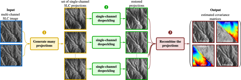
Figure 1: Scheme of the MuChaPro method introduced in this paper, illustrated here on SAR interferometry: multi-channel SAR images are projected into single-channel SLC images which are, after despeckling, recombined to produce the final estimate.

To circumvent the difficulty of building training sets for supervised learning, self-supervised approaches have been proposed for SAR despeckling [dalsasso2022self]. Self-supervised despeckling strategies share a common principle: the splitting of the noisy observations into two subsets, one provided to the despeckling network, the other only available to evaluate the training loss function. Methods differ in the way this splitting is performed:

1. In SAR2SAR [dalsasso2021sar2sar], images captured at different dates are used: a reference date is processed by the network and compared, during training, to a second noisy date. To account for possible changes occurring between these two dates, a change-compensation step is added.

2. Blind-spot approaches [laine2019high] consist of designing a specific network architecture such that the receptive field (i.e., the area in the input image used to predict the value at a given pixel of the output image) excludes the central pixel. The noisy value of that pixel can then be used to evaluate a training loss (the log-likelihood, conditioned by the neighborhood made available to the network). In Speckle2Void [molini2021speckle2void], Molini et al. extend this strategy to SAR despeckling. An alternative is to use more conventional network architectures and apply a preprocessing step to mask out some pixels and use their value to evaluate the training loss, as suggested in [sica2024cohessl].

3. MERLIN [dalsasso2021if] uses the real and imaginary decomposition of a single-look complex SAR image and the property that the speckle in each image of this decomposition is statistically independent of one another (under some assumptions on the SAR transfer function, see [dalsasso2023self]).

A radically different approach is the plug-and-play framework MuLoG [deledalle2017mulog]. Derived from a variational framework and the Alternating Directions Method of Multipliers (ADMM) [boyd2011distributed], it consists first of decomposing a multi-channel SAR image into real-valued channels after a matrix-logarithm is applied to the noisy covariance matrices that capture the polarimetric and/or interferometric information at each pixel, then alternatingly denoising these real-valued channels separately with a conventional graylevel image denoising algorithm (based on a deep neural network or not) and recombining all channels within a non-linear operation. MuLoG presents the advantage of being applicable to SAR images of various dimensionality and to readily include pre-trained networks capable of denoising images corrupted by additive white Gaussian noise. The drawback is the lack of specialization to a specific SAR sensor. In particular, it does not account for the spatial correlations of speckle. Since it is based on the matrix-log decomposition of covariance matrices, some amount of spatial smoothing is necessary, in particular when the dimensionality of the images increases (in multi-baseline interferometry and SAR tomography).

Deep neural networks have been designed specifically to estimate the phase and coherence of an interferometric pair. The $\Phi$-Net [sica2021net] is trained in a supervised way. It applies a decorrelation of the real and imaginary components of the complex interferogram to form the two channels provided as input to the network. InSAR-MONet [vitale2022insar] uses a multi-term loss function to restore the interferometric phase. Digital elevation models and empirical coherence maps were used to generate pairs of simulated noisy/noise-free phase images. The loss combines spatial terms, to ensure that the restored phase is close to the ground-truth phase, and a statistical term to enforce that the estimated noise component follows the expected distribution.

Specific networks have also been proposed for SAR polarimetry, generally following a supervised training methodology. In [DL_polsar_despeck1], the same matrix-logarithm transform as in MuLoG is applied first, then complex-valued operations are applied throughout the network (i.e., the real and imaginary parts are not extracted and processed like a two-channels image but rather complex-convolutions, complex-activations, and complex-batch normalizations are applied). Tucker and Potter [DL_polsar_despeck2] also apply a log-transform but then perform a real-imaginary decomposition and apply a real-valued residual network to estimate the log-transformed speckle component. A different approach is followed in [lin2023residual] where a network is trained, in a supervised way, to produce weights leading to a weighted combination of the neighboring pixels as close as possible to a ground truth. By considering pairs of polarimetric images acquired at close dates, a network is trained without reference in [li2024sentinel]. Unlike SAR2SAR [dalsasso2021sar2sar], no compensation for changes is applied, which could represent a serious limitation in quickly evolving areas (e.g., agricultural fields, changes of soil moisture).

Our contributions: This paper introduces a radically different approach to InSAR and PolSAR despeckling. Although the task requires estimating a multi-dimensional and complex-valued covariance matrix at each pixel, we suggest reducing the problem to a series of single-channel real-valued image despeckling by working on projections, see Figure 1. Such an approach, named “MuChaPro” in the following, presents several advantages:

1. it greatly simplifies the application of deep neural networks for the estimation of polarimetric and / or interferometric properties,

2. a network trained for a given sensor / resolution can be readily applied to various polarimetric or interferometric configurations,

3. it prevents some of the issues occurring with increasing covariance matrix dimensions, in particular, the augmentation of the network complexity required by joint processing of numerous channels and the substantial risk of generalization issues (the spatial polarimetric/interferometric patterns become more diverse and the gap between training and inference steps increases with the dimensionality),

4. the proposed approach is generic: it can accommodate any despeckling algorithm, including deep neural networks of various architectures as well as algorithms that do not use neural networks,

5. various despeckling algorithms can easily be applied in parallel to compare their outputs and get a better sense of possible artifacts / network hallucinations,

6. our approach provides a way to train networks for polarimetric or interferometric despeckling in a self-supervised way.

All those features come at a cost: by reducing the multichannel despeckling problem to a series of independent single-channel despeckling tasks, weakly contrasted geometrical features do not benefit from the reinforcement brought by joint processing. We show in the following that the capacity of most recent self-supervised networks to restore details in single-channel SAR images mitigates this limitation and makes our approach competitive.

II MuChaPro: Estimating covariance matrices from projections

II-A A generic framework for multi-channel restoration using single-channel despeckling techniques

In order to obtain a method that readily generalizes to multi-channel SAR images with an arbitrary number of channels, we propose to project these images into a set of single-channel images and to despeckle these projections. After despeckling, these single-channel images can be recombined to form the final multi-channel covariance estimates. Figure 1 summarizes the principle of our method. Since Multi-Channel Projections are at the core of the framework and we perform many projections (“mucha proyección”, in Spanish), we call our method MuChaPro.

To explain the rationale behind this approach, it is necessary to recall Goodman’s fully-developed speckle model [Goodm]. A single-look complex (SLC) multi-channel SAR image $\boldsymbol{z}$ contains at each pixel $\ell$ a vector $[\boldsymbol{z}]_{\ell}\in\mathbb{C}^{D}$ of $D$ complex amplitudes. Due to speckle, these complex amplitudes are distributed according to a complex circular Gaussian distribution $\mathcal{N}_{c}(\mathbf{C}_{\ell})$ parameterized by the covariance matrix $\mathbf{C}_{\ell}\in\mathbb{C}^{D\times D}$ that contains the polarimetric and/or interferometric information at pixel $\ell$.

Let $\{\boldsymbol{p}_{k}\}_{k=1..K}$ be a set of $K$ vectors of $\mathbb{C}^{D}$. The complex-valued images $\{\boldsymbol{s}_{k}\}_{k=1..K}$ obtained by projection of the multi-channel image $\boldsymbol{z}$ onto the corresponding vectors $\boldsymbol{p}_{k}$ are defined by:

$$\forall\ell,\,[\boldsymbol{s}_{k}]_{\ell}=\boldsymbol{p}_{k}^{\dagger}\cdot[\boldsymbol{z}]_{\ell}\,,$$ (1)

where the notation ${}^{\dagger}$ indicates the conjuguate-transpose operation. The value $[\boldsymbol{s}_{k}]_{\ell}$ is a complex number, i.e., the image $\boldsymbol{s}_{k}$ corresponds to a single-channel SLC image. Since the projection $[\boldsymbol{s}_{k}]_{\ell}$ at pixel $\ell$ corresponds to a linear transform of $[\boldsymbol{z}]_{\ell}$, it also follows a complex circular Gaussian distribution, with a variance equal to $\boldsymbol{p}_{k}^{\dagger}\cdot\mathbf{C}_{\ell}\cdot\boldsymbol{p}_{k}\equiv[\boldsymbol{v}_{k}]_{\ell}\in\mathbb{R}^{+}$. The SLC projections can be seen as regular SAR images, corrupted by single-look speckle, and with an underlying reflectivity $\boldsymbol{v}_{k}$. The application of a single-channel despeckling algorithm separately on each of these images produces estimates $\widehat{\boldsymbol{v}}_{k}$ of the true variance $\boldsymbol{v}_{k}$.

The aim is to recover at each pixel $\ell$ the $D\times D$ covariance matrix $\mathbf{C}_{\ell}$. The definition $[\boldsymbol{v}_{k}]_{\ell}=\boldsymbol{p}_{k}^{\dagger}\cdot\mathbf{C}_{\ell}\cdot\boldsymbol{p}_{k}$ shows that the variances $[\boldsymbol{v}_{k}]_{\ell}$ can themselves be seen as projections of the covariance matrices $\mathbf{C}_{\ell}$:

$$\forall k,\,\forall\ell,\,[\boldsymbol{v}_{k}]_{\ell}=\boldsymbol{q}_{k}^{\dagger}\cdot[\boldsymbol{c}]_{\ell}\,,$$ (2)

with $[\boldsymbol{c}]_{\ell}=\text{vec}(\mathbf{C}_{\ell})$ the vectorized form of $\mathbf{C}_{\ell}$ (i.e., the values of matrix $\mathbf{C}_{\ell}$ are rearranged to form a column vector of dimension $D^{2}$) and vector $\boldsymbol{q}_{k}\in\mathbb{C}^{D^{2}}$ is defined by $\boldsymbol{q}_{k}=\text{vec}(\boldsymbol{p}_{k}\cdot\boldsymbol{p}_{k}^{\dagger})$. In other words, by despeckling the projections $\boldsymbol{z}_{k}$, we recovered projections of the covariances $\mathbf{C}_{\ell}$. It remains to invert these projections, a step that is discussed in the next paragraph.

II-B Recovering the covariance matrix from its projections

The simplest and fastest way to recover, at each pixel $\ell$, the covariance matrix $\mathbf{C}_{\ell}$ consists of solving the following linear least-squares problem:

$$\widehat{\mathbf{C}}_{\ell}\in\mathop{\text{arg min}}_{\mathbf{C}_{\ell}}\sum_{k=1}^{K}\left(\boldsymbol{p}_{k}^{\dagger}\cdot\mathbf{C}_{\ell}\cdot\boldsymbol{p}_{k}-[\widehat{\boldsymbol{v}}_{k}]_{\ell}\right)^{\!2}.$$ (3)

Note that the inversion of the projections is independent from one pixel to the next and can thus be conducted in parallel. Using the notations introduced in equation (2), the least-squares problem can be rewritten in a more conventional form:

$$[\widehat{\boldsymbol{c}}]_{\ell}\in\mathop{\text{arg min}}_{[\boldsymbol{c}]_{\ell}}\left\|\mathbf{Q}^{\dagger}\cdot[\boldsymbol{c}]_{\ell}-[\widehat{\boldsymbol{v}}]_{\ell}\right\|_{2}^{2},$$ (4)

with $\mathbf{Q}$ the $D^{2}\times K$ matrix with the $k$-th column equal to $\boldsymbol{q}_{k}$ and $[\widehat{\boldsymbol{v}}]_{\ell}$ the column vector of the $K$ restored reflectivities at pixel $\ell$ obtained by despeckling the $K$ projections $\{\boldsymbol{s}_{k}\}_{k=1..K}$.

Provided that there are at least $D^{2}$ linearly independent projection directions $\boldsymbol{p}_{k}$, the matrix $\mathbf{Q}\cdot\mathbf{Q}^{\dagger}$ is invertible and the least squares solution is unique and given by:

$$\forall\ell,\,\widehat{\mathbf{C}}_{\ell}^{(\text{MuChaPro})}=\text{vec}^{-1}\!\left(\left(\mathbf{Q}\cdot\mathbf{Q}^{\dagger}\right)^{-1}\cdot\mathbf{Q}\cdot[\widehat{\boldsymbol{v}}]_{\ell}\right),$$ (5)

with $\text{vec}^{-1}$ the reshaping operation that transforms a column vector of size $D^{2}$ back to a $D\times D$ matrix.

input : an $N$-pixels $D$-channels SLC image provided as a matrix $\mathbf{Z}\in\mathbb{C}^{D\times N}$

input : a single-channel despeckling function $f:\;\mathbb{C}^{N}\to\mathbb{R}_{+}^{N}$

output : the restored covariance matrices stored as an $D^{2}\times N$ matrix $\widehat{\mathbf{C}}$ such that the $\ell$-th column contains the $D^{2}$ values of $\text{vec}\bigl{(}\widehat{\mathbf{C}}_{\ell}^{(\text{MuChaPro})}\bigr{)}$, i.e., the covariance matrix at pixel $\ell$ in vectorized form.

Step 1: generate $K$ SLC images by projection

1generate a matrix $\mathbf{P}\in\mathbb{C}^{D\times K}$ whose columns define $K$ projection directions $\{\boldsymbol{p}_{k}\}_{k=1..K}$

2 $\mathbf{S}\leftarrow\mathbf{P}^{\dagger}\cdot\mathbf{Z}$ (compute the $K$ projections)

Step 2: despeckle the projections

for $k=1$ to $K$ do

      3 $\widehat{\mathbf{V}}_{k,\bullet}\leftarrow f(\mathbf{S}_{k,\bullet})$ (despeckle $k$-th single-channel image)

end for

Step 3: recombine restored projections

4build matrix $\mathbf{Q}\in\mathbb{R}^{D^{2}\times K}$ such that $\mathbf{Q}_{\bullet,k}=\text{vec}(\mathbf{P}_{\bullet,k}^{\phantom{\dagger}}\mathbf{P}_{\bullet,k}^{\dagger})$

5 $\widehat{\mathbf{C}}\leftarrow\left(\mathbf{Q}\cdot\mathbf{Q}^{\dagger}\right)^{-1}\!\!\cdot\mathbf{Q}^{\dagger}\cdot\widehat{\mathbf{V}}$ (recover all covariance matrices)

Algorithm 1 MuChaPro, Multi-channel despeckling

The algorithm MuChaPro given at the top of page 1 summarizes the 3 steps of the proposed method by using matrix notation to define each step using linear algebra for an efficient implementation in languages such as Python or Matlab.

The formulation of the least-squares problem (4) does not exploit the Hermitian symmetry of the matrix $\mathbf{C}_{\ell}$. Due to this symmetry, there are not $D^{2}$ complex unknowns but actually $D^{2}$ real unknowns:

$$\mathbf{C}_{\ell}=\begin{pmatrix}\text{C}_{11}&\text{C}_{12}&\cdots&\text{C}_{1D}\\ \text{C}_{12}^{*}&\ddots&\ddots&\vdots\\ \vdots&\ddots&\ddots&\text{C}_{D-1\;D}\\ \text{C}_{1D}^{*}&\cdots&\text{C}_{D-1\;D}^{*}&\text{C}_{DD}\end{pmatrix}$$ (6)

so the vector of all real-valued unknowns $[\boldsymbol{c}]_{\ell}$ at pixel $\ell$ can be structured as follows:

$$[\boldsymbol{c}]_{\ell}=\biggl{(}\text{C}_{11}\;\cdots\;\text{C}_{DD}\;\;\mathbb{R}\text{e}\bigl{(}\text{C}_{12}\bigr{)}\;\cdots\;\mathbb{R}\text{e}\bigl{(}\text{C}_{D-1\;D}\bigr{)}\\ \mathbb{I}\text{m}\bigl{(}\text{C}_{12}\bigr{)}\;\cdots\;\mathbb{I}\text{m}\bigl{(}\text{C}_{D-1\;D}\bigr{)}\biggr{)}^{\!\text{t}}$$ (7)

and the corresponding matrix $\mathbf{Q}$ in equation (4) is structured into 3 blocs:

(8)

(9)

(10)

(12)

(13)

(14)

(16)

(17)

(18)

(19)

wher