RConE: Rough Cone Embedding for Multi-Hop Logical Query Answering on Multi-Modal Knowledge Graphs

Abstract

Multi-hop query answering over a Knowledge Graph (KG) involves traversing one or more hops from the start node to answer a query. Path-based and logic-based methods are state-of-the-art for multi-hop question answering. The former is used in link prediction tasks. The latter is for answering complex logical queries. The logical multi-hop querying technique embeds the KG and queries in the same embedding space. The existing work incorporates First Order Logic (FOL) operators, such as conjunction ($\wedge$), disjunction ($\vee$), and negation ($\neg$), in queries. Though current models have most of the building blocks to execute the FOL queries, they cannot use the dense information of multi-modal entities in the case of Multi-Modal Knowledge Graphs (MMKGs). We propose RConE, an embedding method to capture the multi-modal information needed to answer a query. The model first shortlists candidate (multi-modal) entities containing the answer. It then finds the solution (sub-entities) within those entities. Several existing works tackle path-based question-answering in MMKGs. However, to our knowledge, we are the first to introduce logical constructs in querying MMKGs and to answer queries that involve sub-entities of multi-modal entities as the answer. Extensive evaluation of four publicly available MMKGs indicates that RConE outperforms the current state-of-the-art. The source code and datasets are available at https://github.com/kracr/rcone-qa-mmkg.

I Introduction

A Knowledge Graph (KG) [1] is a directed graph with a set of entities (nodes) and directed relations among those entities (edges). KGs are an excellent tool for representing data in graph topology. They are used in applications such as question-answering and recommendation systems in diverse fields like biomedicine, physics, and geoscience [2].

Multi-hop logical query answering over KGs has gained attention recently [3]. Various neural methods are proposed to answer a logical query. It involves traversing one or more hops over a KG to reach the answers. The query generally consists of First Order Logic (FOL) operators, such as existential quantification ($\exists$), conjunction ($\wedge$), disjunction ($\vee$), and negation ($\neg$).

Current State-of-the-Art (SOTA). There are two major challenges to consider while handling logical query answering over KGs [4]. First, long and complex queries on large KGs incur exponential computational costs. Second, a robust model for handling missing edges in the graphs. Several methods have been proposed to embed the KG and queries in the same space to tackle these issues [5]. These methods iteratively progressed to incorporate different FOL operators in the queries. Geometric [4, 6], and probabilistic [7] methods embed the queries as geometrical shapes and probabilistic distributions, respectively. These methods are scalable and do not keep track of the intermediate nodes.

Shortcomings of SOTA Methods. [RQ1] Multi-Modal Knowledge Graphs (MMKGs) are KGs with multiple modalities, such as images, texts, and videos, as entities [8]. Though the current approaches can handle all the FOL operators well, they cannot incorporate the rich information of multi-modal entities. The node’s embedding, in these models, is based on the relations with its neighbors. They do not consider the entity’s features, which may lead to the loss of critical information in the case of multi-modal entities. [RQ2] There can be multiple subjects in a single multi-modal entity, and it might be that all the subjects are not answers to a query. One of the goals of this work is to get those individual subjects as answers. [RQ3] One way to tackle [RQ1] and [RQ2] is to generate a sub-KG for each multi-modal entity before training (offline). Convert the original MMKG to a non-multi-modal KG by merging all sub-KGs with the MMKG. However, for large MMKGs, constructing the sub-KGs for each multi-modal entity will incorporate high pre-processing and space overhead.

To address these challenges, we propose RConE, an embedding method for answering logical queries on MMKGs. In this work, we focus on entity/relational labels and images as the modalities. We summarize our contributions as follows.

Contribution I: Logical Query Answering on MMKGs at a finer granularity. We propose a novel problem of query answering using FOL constructs on MMKGs. In this problem, the answers might not be complete entities but some part (sub-entities) of the multi-modal entities. To our knowledge, we are the first to handle such queries. Consider the MMKG in Figure 1. For the query, “Shirt color of the actor not wearing brown shoes in the Toy Story movie,” the answer is Green. The related computational graph is in Figure 2. In the MMKG, Green (shirt), is in the Toy Story (Poster) entity (sub-entity of Toy Story (Poster) entity), but there is no entity Green in the MMKG. To cater to these kinds of queries, we propose our model RConE.

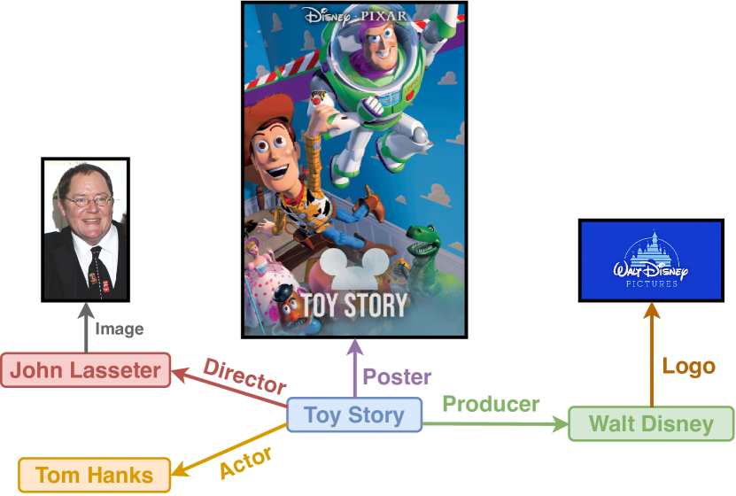
Figure 1: A toy example of a Multi-Modal Knowledge Graph, consisting of images (Toy Story (Poster), John Lasseter (Image), and Walt Disney (Logo)) as a modality, along with regular entities.

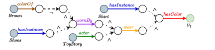
Figure 2: Computational graph for the FOL query $q=V_{\boldsymbol{?}}.\boldsymbol{\exists}V_{1},V_{2},V_{3}:((({\neg\color[rgb]{.75,.5,.25}colorOf}(Brown,V_{1})\boldsymbol{\wedge}{\color[rgb]{0,0,1}hasInstance}(Shoes,V_{1}))\boldsymbol{\wedge}{\color[rgb]{0.55,0.14,1}wornBy}(V_{1},V_{2})\boldsymbol{\wedge}{\color[rgb]{0,0.88,0}actor}(ToyStory,{V_{2}}))\boldsymbol{\wedge}{\color[rgb]{1,.5,0}wear}(V_{2},V_{3})\boldsymbol{\wedge}{\color[rgb]{0,0,1}hasInstance}(Shirt,V_{3}))\boldsymbol{\wedge}{\color[rgb]{1,0,0}hasColor}(V_{3},V_{\boldsymbol{?}})$, corresponding to the question “Shirt color of the actor not wearing brown shoes in the Toy Story movie.” Here nodes represent the entity set, and edges are the logical operations. The green node ($V_{?}$) is the answer to the query.

Contribution II: RConE – A novel perspective of handling the query answering on MMKGs. We extend one of the neural query answering methods, ConE [6], to address the multi-modal entities. The proposed method helps embed entities and sub-entities of an MMKG in the same space where we embed the query.

Contribution III: MMKG Query Generation. We extend a logical query generation algorithm [7] to incorporate the multi-modal entities/sub-entities while generating the training queries. We create queries based on 14 structures described in the literature.

Contribution IV: Extensive Evaluation. We extensively test our method over four multi-modal datasets. The difference between RConE and the best-performing baseline is $56.5\%$ in the MRR score for one of the datasets.

II Related Work

Multi-Hop Query Answering. There are two types of multi-hop querying techniques: path-based answering [9, 10, 11, 12, 13, 14] and logical query answering. In path-based answering, rules or paths of the KG are traversed to answer a query. It is generally used to improve the link prediction task. Logical query answering [5] embeds the KG and the query in the same space to evaluate the answer set. Our proposed model is based on logical query answering.

GQE [15] proposed the initial query engine. The model answers the query with the closest answer embedded to the query. Query2Box [4] extended the work by representing the region of interest (ROI) using d-dimensional boxes. This ROI helps incorporate multiple answers to a query. The model could handle the disjunction ($\vee$) and conjunction ($\wedge$) operators. BetaE [7] and ConE [6] extended Query2Box to integrate the negation ($\neg$) operator, making them fully compatible with FOL operators. While BetaE uses $d$-beta distributions to represent a query component, ConE uses $d$-ary sector cones. Extensions have also been proposed for hyper-relational KGs [16, 17] and temporal KGs [18]. A detailed survey on different query-answering methods is provided in [19]. Information about the current state of the art and the prospective future of logical query answering over KGs is contemplated in [5].

Question-Answering on MMKGs. There are several works on path-based question-answering over an MMKG. Single-hop models like IKRL [20] use attention to capture the visual features of images. TransAE [21] adds multi-modal features and extends the conventional single-hop embedding model TransE [22]. MMKGR [23] proposed the initial multi-hop path-based query answering method using reinforcement learning for a unified gate attention network to filter noise. A review of the application of MMKGs in different fields is presented in [8]. Though these works use MMKGs to evaluate a query, they do not support logical queries with FOL constructs.

III Preliminaries

MMKG. A Multi-Modal Knowledge Graph $G(\mathcal{V},\mathcal{R},\mathcal{U},\mathcal{M})$ is a directed graph where $\mathcal{V}$ and $\mathcal{R}$ are entity and relation sets, respectively. $\mathcal{U}$ is the triplet set, represented as

$$\mathcal{U}=\{(e_{s},r,e_{d})\;\;|\;\;e_{s},e_{d}\in\mathcal{V},r\in\mathcal{R}\}$$ (1)

There are $|\mathcal{M}|=k$ modalities in the graph, such that

$$\gamma(e_{i})\in\mathcal{M}=\{m_{1},m_{2},\ldots,m_{k}\},e_{i}\in\mathcal{V}$$ (2)

where $m_{1}$ is the generic entity label. In Figure 1, the entities $\{$Tom Hanks, Walt Disney$\}\in m_{1}$ (generic) and $\{$Toy Story (Poster), Walt Disney (Logo)$\}\in m_{2}$ (images). We consider $k=2$, in this work.

Sub-Entity Knowledge Graph (Scene Graph). For each node, $e_{j}$, such that $\gamma(e_{j})=m_{2}$, we define a sub-entity KG or a scene graph as $SG_{j}(\mathcal{V}_{j},\mathcal{R}_{j},\mathcal{U}_{j})$. $\mathcal{V}_{j}$, $\mathcal{R}_{j}$, and $\mathcal{U}_{j}$ are sub-entity, sub-relation, and sub-triplet sets, respectively. The $SGs$ are the KGs describing each multi-modal entity in $G$.

FOL Queries. First Order Logic (FOL) queries $q\in Q=\{Q_{train},Q_{test}\}$ consists of logical operators such as conjunction ($\wedge$), disjunction ($\vee$), existential quantification ($\exists$), and negation ($\neg$). We are not including universal quantification ($\forall$), similar to [7, 6], as its applications in real-world KGs are rare. Queries are expected to be in Disjunctive Normal Form (DNF). This enables us to handle the union operator at the end, which helps the model to be scalable for long queries. An FOL query $q\in Q$, with respect to an MMKG, comprises a non-variable anchor entity set

$$\mathcal{V}_{a}\subseteq\mathcal{V_{\cup}}=\Biggl{\{}\bigcup_{j=1}^{|\mathcal{V}|}\mathcal{V}_{j}\cup\mathcal{V}\bigm{|}\gamma(e_{j})=m_{2}\Biggr{\}}$$ (3)

along with existentially quantified bound variables $V_{1},\ldots,V_{k}$ and a target variable $V_{?}$ (query’s answer). The DNF for the query is

$$q[V_{?}]=V_{?}.\exists V_{1},\dots,V_{k}:c_{1}\vee c_{2}\vee...\vee c_{n}$$ (4)

with $c_{i}=\{l_{i1}\wedge l_{i2}\wedge...\wedge l_{il}\}$, being conjunctions of one or more literals $l$, such that $l_{ij}=r(v_{a},V)$ or $\neg r(v_{a},V)$ or $r(V^{\prime},V)$ or $\neg r(V^{\prime},V)$, where $v_{a}\in\mathcal{V}_{a}$, $V\in\{V_{?},V_{1},\ldots,V_{k}\}$, $V^{\prime}\in\{V_{1},...,V_{k}\}$, $V\neq V^{\prime}$, and $r\in\mathcal{R}_{\cup}=\{\bigcup_{j=1}^{|\mathcal{V}|}\mathcal{R}_{j}\cup\mathcal{R}\;|\;\gamma(e_{j})=m_{2}\}$.

The objective of a FOL query answering model for an MMKG is

$$\theta^{\prime}=\arg\min_{\theta}\sum_{q\in Q_{test}}\mathcal{L}(g_{\theta}(G,q),g_{\theta}(\mathcal{A}_{gt}(q)))$$ (5)

Here, $\theta$ is the set of parameters for the embedding module $g$, $\mathcal{A}_{gt}(q)$ is the ground-truth answer set of query $q$, and $\mathcal{L}$ is the loss function.

Query Answer Types. Through RConE, we will handle two sets of answers to a query. Type (I) answers: For query Q1 – “Shirt color of the actor not wearing brown shoes in the Toy Story movie,” while there is no entity for the color Green in $\mathcal{V}$ (Figure 1), it can be extracted from the multi-modal entity, the Toy Story (Poster). Hence, it is a sub-entity (not an entity) answer in MMKG. Type (II) answers: For query Q2 – “Director of the movie Toy Story.” we have an entity, John Lasseter, in $G$. Hence, the complete entity is the answer to the query.

Computational Graphs. A computational graph illustrates a complex logical query through a graph, as shown in Figure 2. Nodes symbolize the distribution of entities, and edges denote the transformations of this distribution. It helps to propagate queries through the KG. We can construct the graph from the query by converting the relation propagation to the projection operations, conjunction to the intersection of sets, negation to complement, and disjunction to the union of the entity distribution.

Rough Convex Cone. Here, we discuss the use of the rough convex cone to embed the MMKG.

Definition 1

[24] A subset $C\in\mathbb{R}^{2}$ is called a cone if, $\forall x\in C$, $\alpha\in\mathbb{R}_{\geq 0}$, $\alpha x\in C$. A cone is convex if, $\forall x_{1},x_{2}\in C$ and $\lambda_{1},\lambda_{2}\in\mathbb{R}_{\geq 0}$, we have $\lambda_{1}x_{1}+\lambda_{2}x_{2}\in C$.

Previous method proposed sector cone for embedding a (non-multi-modal) KG [6].

Definition 2

A 2D closed cone is called a sector-cone, if its closure-complement or itself is convex.

Definition 3

The closure-complement of cone $C\subset\mathbb{R}^{2}$ is defined by $\tilde{C}=cl(\mathbb{R}^{2}\setminus C)$, where $cl(.)$ is the closure of a set.

To handle MMKGs, we extend the convex cones to rough convex cones.

Definition 4

[25] Let $W$ be a subspace of a space $S$, for $\alpha,\beta\in S$, $\alpha$ and $\beta$ are congruence with respect to $W$ ($\alpha\in R_{w}(\beta)$), if $\alpha-\beta\in W$. Here, $R_{w}(\beta)$ is the equivalence class containing the element $\beta$.

Definition 5

[25] The rough approximation of a non empty answer set $X\subseteq S$, is defined as $R_{w}X=(\underline{R_{w}}X,\overline{R_{w}}X)$, where,

$$\underline{R_{w}}X =\{x\in S\mid R_{w}(x)\subseteq X\}$$ (6a)

$$\overline{R_{w}}X =\{x\in S\mid R_{w}(x)\cap X\neq\emptyset\}$$ (6b)

$\underline{R_{w}}X$ and $\overline{R_{w}}X$ are lower and upper rough approximations of $X$, respectively. $X$ is called a $R_{w}$-rough convex cone if both $\underline{R_{w}}X$ and $\overline{R_{w}}X$ are convex cones. $R_{w}NX=\overline{R_{w}}X-\underline{R_{w}}X$ is the fuzzy boundary region.

Membership function in a rough set [26] is defined as

$$\mu_{X}^{R_{w}}(x)=1, \text{\hskip 20.0pt iff }x\in\underline{R_{w}}X$$ (7a)

$$\mu_{X}^{R_{w}}(x)=0, \text{\hskip 20.0pt iff }x\in S-\overline{R_{w}}X$$ (7b)

$$0<\mu_{X}^{R_{w}}(x)<1, \text{\hskip 20.0pt iff }x\in R_{w}NX$$ (7c)

In MMKG, let all the entities $e\in\mathcal{V}$ are equivalent classes. For Q1, Toy Story (Poster) $\in\overline{R_{w}}X$ since at least one sub-entity of the entity belongs to the answer set (green), while Toy Story (Poster) $\notin\underline{R_{w}}X$ as not all of its sub-entities belong to the answer set. Similarly, in Q2, John Lasseter $\in\underline{R_{w}}X$, since the entire entity is an answer to the query.

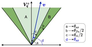
Figure 3: RConE embedding for a query, $\boldsymbol{V_{q}^{c}}=(\theta_{ax},\theta_{ri},\theta_{fu})$, in $2$-dimension, with $\theta_{ax}$ being the angle between the co-ordinate axis and axis of the embedding. The region A (light green) across the axis is the rigid region ($\theta_{ri}$), and the region B (dark green) resembles the fuzzy (boundary) region ($\theta_{fu}$). The blue vector is the entity embedding ($\boldsymbol{v}=(\theta_{ax},0,0)$).

RConE Representation. The sector-cone is always axially symmetric, we can represent a $2$-dimensional sector-cone using a pair of parameters $(\theta_{ax},\theta_{ri})$, where $\theta_{ax}$ is the axis and $\theta_{ri}$ is the aperture [6]. We use the idea of the rough convex cone, and present a two-dimensional RConE as a triplet $(\theta_{ax},\theta_{ri},\theta_{fu})$ (Figure 3). We have $\theta_{ri}\in[0,2\pi]$ as the rigid aperture, for lower approximation ($\underline{R_{w}}X$). $\theta_{fu}\in[0,2\pi-\theta_{ri}]$ is the extended fuzzy (boundary) region ($R_{w}NX$) along both sides of the rigid sector cone. $\theta_{ax}\in[-\pi,\pi)$ is an axis shared by both cones. Consider RConE as two overlapping sector cones ($\underline{R_{w}}X$ and $\overline{R_{w}}X$) sharing a common semantic axis. All the points in the range $[\theta_{ax}-\theta_{ri}/2,\theta_{ax}+\theta_{ri}/2]$ would belong to the rigid sector cone, while all the points in $[\theta_{ax}-(\theta_{ri}+\theta_{fu})/2,\theta_{ax}-\theta_{ri}/2]\cup[\theta_{ax}+\theta_{ri}/2,\theta_{ax}+(\theta_{ri}+\theta_{fu})/2]$, would be in the fuzzy boundary sector cone.

We can represent a RConE as $R_{0}=(\theta_{ax},\theta_{ri},\theta_{fu})\in\mathbb{K}$, where $\mathbb{K}$ is the space containing all triplets $(\theta_{ax},\theta_{ri},\theta_{fu})$. The $d$-ary Cartesian product of RConE can be presented as

$$R=((\theta_{ax}^{1},\theta_{ri}^{1},\theta_{fu}^{1}),\ldots(\theta_{ax}^{d},\theta_{ri}^{d},\theta_{fu}^{d}))\subset\mathbb{K}^{d}$$ (8)

or $R=(\boldsymbol{\theta}_{ax},\boldsymbol{\theta}_{ri},\boldsymbol{\theta}_{fu})$, with $\boldsymbol{\theta}_{ax}=\{\theta_{ax}^{1},\ldots,\theta_{ax}^{d}\}\in[-\pi,\pi)^{d}$, $\boldsymbol{\theta}_{ri}=\{\theta_{ri}^{1},\ldots,\theta_{ri}^{d}\}\in[0,2\pi]^{d}$, and $\boldsymbol{\theta}_{fu}=\{\theta_{fu}^{1},\ldots,\theta_{fu}^{d}\}\in[0,2\pi-\theta_{ri}]^{d}$.

IV Method

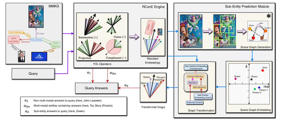
Figure 4: Our proposed framework, RConE: The first sub-module, RConE Engine (RCE), embeds the input query and Multi-Modal Knowledge Graph (MMKG) to the embedding space (resultant embeddings). Then, the Sub-Entity Prediction module generates the sub-entity embeddings from the candidate multi-modal entities in the fuzzy region (dark blue region in resultant embeddings), using three sub-modules – Scene Graph Generation, Scene Graph Embedding and Graph Transformation.

Figure 4 presents the flow diagram of our model RConE. It comprises two modules, the RConE Engine (RCE) and the Sub-Entity Prediction module. The RCE traverses query and outputs two entity sets – 1) Answer entities in the rigid region (John Lassester in Q2). 2) Multi-modal entities consisting of the answers in the fuzzy region (Toy Story (Poster) in Q1). For each candidate multi-modal entity in the fuzzy region (here, Toy Story (Poster)), the Sub-Entity Prediction module initially generates a sub-entity KG (scene graph). Following this, it embeds the scene graph. Finally, the module transforms the sub-entities to the RConE’s embedding space. The transformation is such that the answer sub-entities (Green in Q1) belong in the rigid region and other sub-entities outside the RConE embedding. In the following subsections, we describe each module in detail. A brief overview of the steps is presented in Algorithm 1 in the supplementary material.

IV-A RConE Engine (RCE)

As shown in Figure 4, RCE takes MMKG and queries as input and embeds them in the RConE embedding space. It traverses the query computational graph to generate the embedding. During traversal, RCE handles different FOL operators in a query. We first discuss the embedding procedure for queries and entities. Following it are the details about the transformation in embeddings based on the FOL operators.

Entity and Query Embedding. Let $\mathcal{A}(q)$ be the entity set satisfying the query $q$. The embedding for $\mathcal{A}(q)$ is the cartesian product of $d$-ary (fuzzy-rigid) sector cones in $\mathbb{K}^{d}$ embedding space (Figure 3). The embedding is presented as $\boldsymbol{V}^{c}_{q}=(\boldsymbol{\theta}_{ax},\boldsymbol{\theta}_{ri},\boldsymbol{\theta}_{fu})$, where $\boldsymbol{\theta}_{ax}\in[-\pi,\pi)^{d}$ is the semantic axis. $\boldsymbol{\theta}_{ri}\in[0,2\pi]^{d}$ is the rigid aperture enclosing the region $A$ around it. $\boldsymbol{\theta}_{fu}\in[0,2\pi-\theta_{ri}]^{d}$ is the fuzzy aperture enclosing region $B$ around the rigid cone.

All entities belonging to the answer set (John Lasseter in Q2) will have embeddings in the region $A$. The multi-modal entities in $G$, which have some part in the answer (Toy Story (Poster) in Q1), will have embeddings in region $B$.

The embedding of node $v\in\mathcal{V}_{\cup}$ is represented as $\boldsymbol{v}=(\boldsymbol{\theta}_{ax},\boldsymbol{0},\boldsymbol{0})$. It can be considered as an answer set consisting of a single answer $v$. The embedding consists of no rigid and fuzzy areas (blue vector in Figure 3).

The reasons we are using the rough sets (fuzzy (boundary) region) as an extension to the original ConE [6] model are

• The multi-modal entities should operate in the same space as the unimodal entities as we are traversing the query in that space.

• The multi-modal entities containing the answer would be semantically similar to other answers. So, their embedding should also be closer. Hence, they would belong to the boundary region with partial membership (Equation 7c) to the answer set.

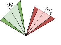
(a)

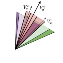
(b)

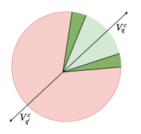
(c)

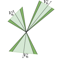
(d)

Figure 5: A representation of the impact of different logical operators in RConE Engine (RCE) ($1$-ary). Here (for (a) projection, (b) intersection, and (c) complement operators), $\boldsymbol{V}^{c}_{q_{i}}$ is the input RConE embedding(s) to the operator, and $\boldsymbol{V}^{c}_{q^{\prime}}$ is the output embedding. In the (d) union operator, the output is all the input embeddings ($\boldsymbol{V}^{c}_{q_{i}}$).

Logical Operators. The query computational graph consists of different logical operators (Intersection, Union, and Complement) along with the relation projection operator. The $\mathcal{A}(q)$’s RConE embedding resembles the answer set that satisfies the processed query at any moment through this traversal. Figure 5 consists of the visual representation of how all the operations work on $1$-ary RConE embedding. We present the modeling of each operator below. Each operator has been extended to accomodate the fuzzy boundary part in ConE[6].

Projection. Projection is a relation-dependent transformation of answer distribution ($\mathcal{A}(q)$), with the transformed embedding in the same space as the original one. We define projection mapping using the following function.

$$\mathcal{P}_{r}:\boldsymbol{V}^{c}_{q}\mapsto\boldsymbol{V}^{c}_{q^{\prime}},\;\;\;\boldsymbol{V}^{c}_{q},\boldsymbol{V}^{c}_{q^{\prime}}\in\mathbb{K}^{d}$$ (9)

We can consider projection as the shift in cones’ angles based on the relation encountered. Given the relation embedding as $\boldsymbol{r}=(\boldsymbol{\theta}_{ax,r},\boldsymbol{\theta}_{ri,r},\boldsymbol{\theta}_{fu,r})$, the transformed cone would be dependent on $\boldsymbol{\theta}_{ax}+\boldsymbol{\theta}_{ax,r},\boldsymbol{\theta}_{ri}+\boldsymbol{\theta}_{ri,r}$ and $\boldsymbol{\theta}_{fu}+\boldsymbol{\theta}_{fu,r}$. We use an MLP of this tranformed cone to describe the projection, as presented below.

$$=[\boldsymbol{\theta^{\prime}}_{ax};\boldsymbol{\theta^{\prime}}_{ri};\boldsymbol{\theta^{\prime}}_{fu}]$$

Here $[.;.;.]$ concatenates the three vectors, and $\sigma_{P}$ (Tanh) keeps the output in the required range for all the $\theta$s (Equation 11).

$[\sigma_{P}(x)]_{i}$ represents the $i$-th value of $\sigma_{P}(x)$. $\lambda_{j}$’s being the parameters to scale. Though Tanh has a range $(-1,1)$, which may lead to never getting the boundary values. However, approximations due to hardware constraints can lead to these values as well.

Intersection. If we have $n$ query answer sets, denoted as $\mathcal{A}(q_{1}),\ldots,\mathcal{A}(q_{n})$ with RConE embeddings $\boldsymbol{V}_{q_{1}}^{c},\ldots,\boldsymbol{V}_{q_{n}}^{c}$, respectively. We aim to identify the intersection query answer set $\mathcal{A}(q^{\prime})$ by finding the shared region among these embeddings (Figure 5b). The modified parameters can be expressed as.

$$\boldsymbol{\theta^{\prime}}_{ax} =SemanticAverage(\boldsymbol{V}_{q_{1}}^{c},\ldots,\boldsymbol{V}_{q_{n}}^{c})$$

$$\boldsymbol{\theta^{\prime}}_{ri} =RigidAverage(\boldsymbol{V}^{c}_{q_{1}},\ldots,\boldsymbol{V}^{c}_{q_{n}})$$

$$\boldsymbol{\theta^{\prime}}_{fu} =FuzzyAverage(\boldsymbol{V}^{c}_{q_{1}},\ldots,\boldsymbol{V}^{c}_{q_{n}})$$

For $i$-th input embedding $\boldsymbol{V}^{c}_{q_{i}}$, let $\mathcal{B}_{i}$ be defined as

$$\mathcal{B}_{i}= [\boldsymbol{\theta}_{ax}-\boldsymbol{\theta}_{ri}/2;\boldsymbol{\theta}_{ax}+\boldsymbol{\theta}_{ri}/2;$$

$$\boldsymbol{\theta}_{ax}-(\boldsymbol{\theta}_{ri}+\boldsymbol{\theta}_{fu})/2;\boldsymbol{\theta}_{ax}+(\boldsymbol{\theta}_{ri}+\boldsymbol{\theta}_{fu})/2]_{i}$$ (12)

SemanticAverage. The final aperture $\boldsymbol{\theta^{\prime}}_{ax}$ depends on the average of the intersecting cones’ semantic centers. Similar to [6], our method employs an attention module $[\boldsymbol{a}]$ to characterize the semantic center based on each input’s rigid and fuzzy region. We utilize the relation below to calculate the attention mechanism.

$$[\boldsymbol{a}]=\sigma_{s2}(W_{s2}\sigma_{s1}(W_{s1}\mathcal{B}))$$ (13)

Here, $\sigma_{s1}$ and $\sigma_{s2}$ represent the ReLU and softmax functions, respectively.

The resultant semantic center is determined by mapping the input axes to a unit circle, performing a weighted average of all the semantic centers (using the attention module), and reverting the points to their original form. The following relations describe this process.

$$[\boldsymbol{x};\boldsymbol{y}]= \sum_{i=1}^{n}[\boldsymbol{a}_{i}\circ cos(\boldsymbol{\theta}_{i,ax});\boldsymbol{a}_{i}\circ sin(\boldsymbol{\theta}_{i,ax})]$$ (14)

$$\boldsymbol{\theta^{\prime}}_{ax}= \sigma_{s}(\boldsymbol{x},\boldsymbol{y})$$ (15)

Here, $\sigma_{s}$ is used to transform all the values into the required range as,

$$[\boldsymbol{\theta^{\prime}}_{ax}]_{i}=\begin{cases}\arctan([\boldsymbol{y}]_{i}/[\boldsymbol{x}]_{i})+\pi,&if[\boldsymbol{x}]_{i}<0,[\boldsymbol{y}]_{i}>0,\\ \arctan([\boldsymbol{y}]_{i}/[\boldsymbol{x}]_{i})-\pi,&if[\boldsymbol{x}]_{i}<0,[\boldsymbol{y}]_{i}<0,\\ \arctan([\boldsymbol{y}]_{i}/[\boldsymbol{x}]_{i}),&otherwise\end{cases}$$ (16)

RigidAverage. Let $\boldsymbol{V}_{q_{X}}^{c}$ and $\boldsymbol{V}_{q_{Y}}^{c}$ be two input answer set embeddings, with rough sets $R_{w}X$ and $R_{w}Y$, respectively. The rigid region of the resultant answer set from the intersection operation [26] is defined as

$$\underline{R_{w}}(X\cap Y)=\underline{R_{w}}X\cap\underline{R_{w}}Y$$ (17)

where $\underline{R_{w}}X$ and $\underline{R_{w}}Y$ are the rigid regions of the input rough sets $R_{w}X$ and $R_{w}Y$, respectively. Hence, the resultant RConE embedding’s rigid aperture $\boldsymbol{\theta^{\prime}}_{ri}$ should be the subset of all intersecting apertures of $\boldsymbol{V}^{c}_{q_{1}},\ldots,\boldsymbol{V}^{c}_{q_{n}}$ presented as Equation 18 (similar to [6]).

$$\boldsymbol{\theta^{\prime}}^{i}_{ri}=\min\{\boldsymbol{\theta}_{1,ri}^{i},...,\boldsymbol{\theta}_{n,ri}^{i}\}.\sigma([DeepSets(\{\boldsymbol{V}_{q_{j}}\}^{n}_{j=1})]_{i})$$ (18)

Here, deep sets (Equation 19) is an MLP to learn the intersecting answer sets’ context.

$$MLP\left(\frac{1}{n}\sum_{j=1}^{n}MLP(\mathcal{B})\right)$$ (19)

FuzzyAverage. Unlike the RigidAverage, the resultant fuzzy borders depend on the intersection of fuzzy-fuzzy regions and the fuzzy-rigid regions both, for two or more input answer sets. Let $\boldsymbol{V}_{q_{X}}^{c}$ and $\boldsymbol{V}_{q_{Y}}^{c}$ be two input answer set embeddings, with rough sets $R_{w}X$ and $R_{w}Y$, respectively. The upper rough approximation of the resultant answer set from the intersection operation [26] is defined as

$$\overline{R_{w}}(X\cap Y)\leq\overline{R_{w}}X\cap\overline{R_{w}}Y$$ (20)

where $\overline{R_{w}}X$ and $\overline{R_{w}}Y$ are the upper rough approximation of the input rough sets $R_{w}X$ and $R_{w}Y$, respectively. Since $\overline{R_{w}}X=R_{w}NX+\underline{R_{w}}X$, we can deduce the following relation for the output RConE embedding,

$$(\boldsymbol{\theta^{\prime}}^{i}_{fu}+\boldsymbol{\theta^{\prime}}^{i}_{ri})\leq\min\{(\boldsymbol{\theta}_{1,fu}^{i}+\boldsymbol{\theta}_{1,ri}^{i}),...,(\boldsymbol{\theta}_{n,fu}^{i}+\boldsymbol{\theta}_{n,ri}^{i})\}$$ (21)

We opt for a trivial boundary as well that the resultant fuzzy area would not be greater than the maximum fuzzy region,

$$\boldsymbol{\theta^{\prime}}^{i}_{fu}\leq\max\{\boldsymbol{\theta}_{1,fu}^{i},...,\boldsymbol{\theta}_{n,fu}^{i}\}$$ (22)

From Equation 21 and 22, we can construct the following relation for the resultant fuzzy boundary,

$$\boldsymbol{\theta^{\prime}}^{i}_{fu}=\sigma([DeepSets]).\min\{\max\{\boldsymbol{\theta}_{1,fu}^{i},...,\boldsymbol{\theta}_{n,fu}^{i}\},$$ (23)

$$\min\{(\boldsymbol{\theta}_{1,fu}^{i}+\boldsymbol{\theta}_{1,ri}^{i}),...,(\boldsymbol{\theta}_{n,fu}^{i}+\boldsymbol{\theta}_{n,ri}^{i})\}-\boldsymbol{\theta^{\prime}}^{i}_{ri}\}$$

where $\boldsymbol{\theta^{\prime}}^{i}_{ri}$ is the updated rigid aperture, and DeepSets here is similar to that described in the RigidAverage.

Complement. The semantic axis for the resultant embedding ($\boldsymbol{V}_{q^{\prime}}^{c}$) from the complement operator will be in the opposite direction to the input embedding ($\boldsymbol{V}_{q}^{c}$) (Figure 5c). The new axis is described as

$$[\boldsymbol{\theta^{\prime}}_{ax}]_{i}=\begin{cases}[\boldsymbol{\theta}_{ax}]_{i}-\pi,&\text{if }[\boldsymbol{\theta}_{ax}]_{i}\geq 0,\\ [\boldsymbol{\theta}_{ax}]_{i}+\pi,&\text{if }[\boldsymbol{\theta}_{ax}]_{i}<0\end{cases}$$ (24)

The rigid region’s angle of $\boldsymbol{V}_{q^{\prime}}^{c}$ ($\boldsymbol{\theta^{\prime}}_{ri}$) will be all the $2\pi$ region except the area covered by the input rigid ($\boldsymbol{\theta}_{ri}$) and fuzzy sector cone ($\boldsymbol{\theta}_{fu}$), that is,

$$[\boldsymbol{\theta^{\prime}}_{ri}]_{i}=2\pi-([\boldsymbol{\theta}_{ri}]_{i}+[\boldsymbol{\theta}_{fu}]_{i})$$ (25)

For complement operation, the fuzzy embedding would be identical for both $\boldsymbol{V}_{q}^{c}$ and $\boldsymbol{V}_{q^{\prime}}^{c}$ (the dark green region in Figure 5c). For a multi-modal entity $e$ belonging to the fuzzy area, if membership to the input embedding, $\boldsymbol{V}_{q_{X}}^{c}$, is $\mu_{X}^{R_{w}}(e)=k$, with $0<k<1$. After complement operation, it would be $\mu_{X^{\prime}}^{R_{w}}(e)=(1-k)$. So,

$$[\boldsymbol{\theta^{\prime}}_{fu}]_{i}=[\boldsymbol{\theta}_{fu}]_{i}$$ (26)

Union. Handling the union operator at the end makes the model scalable [7]. We convert the queries to the DNF form for execution. Suppose $\boldsymbol{V}_{q_{i}}^{c}=(\boldsymbol{\theta}_{i,ax},\boldsymbol{\theta}_{i,ri},\boldsymbol{\theta}_{i,fu})$ is the $i$th input RConE embeddings. The union of all the input embeddings [6] would be

$$\boldsymbol{V}_{q}^{c}=\{\boldsymbol{V}_{q_{1}}^{c},\ldots,\boldsymbol{V}_{q_{n}}^{c}\}$$ (27)

it can also be represented as

$$\leavevmode\resizebox{381.5877pt}{}{$\boldsymbol{V}_{q}^{c}=(\{(\boldsymbol{\theta}_{1,ax}^{1},\boldsymbol{\theta}_{1,ri}^{1},\boldsymbol{\theta}_{1,fu}^{1}),\ldots,(\boldsymbol{\theta}_{n,ax}^{1},\boldsymbol{\theta}_{n,ri}^{1},\boldsymbol{\theta}_{n,fu}^{1})\},$}$$ (28)

$$\leavevmode\resizebox{381.5877pt}{}{$\ldots,\{(\boldsymbol{\theta}_{1,ax}^{d},\boldsymbol{\theta}_{1,ri}^{d},\boldsymbol{\theta}_{1,fu}^{d}),\ldots,(\boldsymbol{\theta}_{n,ax}^{d},\boldsymbol{\theta}_{n,ri}^{d},\boldsymbol{\theta}_{n,fu}^{d})\})$}$$

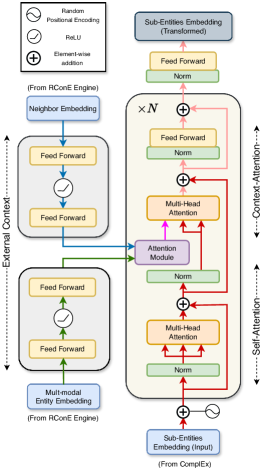
Figure 6: Graph Transformation: It transforms the sub-entities from the Scene Graph Embedding (ComplEx) space to the RConE embedding space. It uses the multi-modal entity and its neighbor embedding from RCE in the attention module for external context. The input and output of the sub-module are highlighted in blue and grey, respectively.

IV-B Sub-Entity Prediction

After passing through the RConE Engine, we receive entity sets belonging to the rigid region (John Lassester in Q2) and fuzzy region (Toy Story (Poster) in Q1). The Sub-Entity Prediction module takes candidate multi-modal entities from the fuzzy region (here, Toy Story (Poster)) as input. It returns the embedding of the answer sub-entity Green in the rigid region and other non-answer sub-entities outside the RConE embedding. The module consists of three parts: Scene Graph Generation, Scene Graph Embedding, and Graph Transformation (Figure 4). We present details of each sub-module below.

Scene Graph Generation. The sub-module creates a scene graph for each candidate multi-modal entity (here, Toy Story (Poster)). The sub-model is trained on a large scene-graph dataset and is used in RConE in a zero-shot manner to generate scene graphs. We use FCSGG [27] as our scene graph generation algorithm.

Scene Graph Embedding. This sub-module embeds the scene graph of each image received from the last sub-module in an embedding space. The embedding is based on the relations within that image to incorporate the context of the image. We use ComplEx [28] to embed the scene graph.

Graph Transformation. In the last step, we transform all the sub-entity embeddings of each scene graph embedding to the RConE embedding space. The sub-module is based on the transformer [29] (Figure 6). In each layer, we have two multi-head attentions. The first attention is for the context of other sub-entities in the same multi-modal entity (each sub-entity of Toy Story (Poster)). The second multi-head attention is for the context of the multi-modal entity and its n-hop neighbors (embedding of Toy Story (Poster), and its neighbors) from RCE. The attention [30] coefficients for external context are calculated in the attention module (Figure 6) as

$$h_{e}^{0}\leftarrow\boldsymbol{v}_{m}$$ (30)

where $\boldsymbol{v}_{m}$ is the candidate multi-modal entity, and $N(\boldsymbol{v}_{m})$ is the set of $\boldsymbol{v}_{m}$’s neighbor entities.

IV-C Loss Function

TABLE I: Description of variables used in loss function.

Lower border	Upper border
$\boldsymbol{\theta}_{L_{ri}}=\boldsymbol{\theta}_{ax}-\boldsymbol{\theta}_{ri}/2$	$\boldsymbol{\theta}_{U_{ri}}=\boldsymbol{\theta}_{ax}+\boldsymbol{\theta}_{ri}/2$
$\boldsymbol{\theta}_{L_{fu}}=\boldsymbol{\theta}_{ax}-(\boldsymbol{\theta}_{ri}+\boldsymbol{\theta}_{fu})/2$	$\boldsymbol{\theta}_{U_{fu}}=\boldsymbol{\theta}_{ax}+(\boldsymbol{\theta}_{ri}+\boldsymbol{\theta}_{fu})/2$
$\boldsymbol{\theta}_{Lm_{fu}}=\boldsymbol{\theta}_{ax}-(\boldsymbol{\theta}_{ri}/2+\boldsymbol{\theta}_{fu}/4)$	$\boldsymbol{\theta}_{Um_{fu}}=\boldsymbol{\theta}_{ax}+(\boldsymbol{\theta}_{ri}/2+\boldsymbol{\theta}_{fu}/4)$

There are two goals while constructing the loss function.

1. For Type (I) answers, $e\in\mathcal{V}_{j}$ ($e_{j}\in\mathcal{V}\;|\;\gamma(e_{j})=m_{2}$), we require the embedding of the nodes

   1. $e_{j}$ (multi-modal entities) in the fuzzy region of RConE (Toy Story (Poster) in Q1).

   2. $e$ (the sub-entity answer) inside the rigid border of RConE (Green in Q1).

2. For Type (II) answers, $e\in\mathcal{V}$, we require the embedding of the nodes within the rigid borders of RConE (John Lasseter in Q2).

All other (sub) entities’ embeddings in $\mathcal{V}$ and $\mathcal{V}_{j}$ should be outside RConE. We define the loss function as

$$L=L_{c}+\lambda_{l1}L_{se}+\lambda_{l2}L_{mm}$$ (31)

Here, $L_{c}$ is the loss for Type (II) answers $e$ in $\mathcal{V}$ (goal 2), $L_{se}$ is for the sub-entity in Type (I) answers $e$ in $\mathcal{V}_{j}$ (goal 1b), and $L_{mm}$ is for the multi-modal entities ($e_{j}$) in Type (I) answers (goal 1a). $\lambda_{l1}$ and $\lambda_{l2}$ are hyper-parameters. We use negative sampling loss in each case, as described by Equation 32.

$$L_{neg}= -\log\sigma(\gamma-d(\boldsymbol{v};\boldsymbol{V}^{c}_{q}))-\frac{1}{k}\sum_{i=1}^{k}\log\sigma(d(\boldsymbol{v^{\prime}}_{i};\boldsymbol{V}^{c}_{q})-\gamma)$$ (32)

Here $\boldsymbol{v}$ and $\boldsymbol{v^{\prime}}$ are positive and negative samples, respectively. $d(\boldsymbol{v};\boldsymbol{V}_{q}^{c})$ is the distance between the node $\boldsymbol{v}$ and query answer set embedding, $\boldsymbol{V}_{q}^{c}$ formulated as

$$d(\boldsymbol{v};\boldsymbol{V}^{c}_{q})=\begin{cases}d_{con}(\boldsymbol{v};\boldsymbol{V}^{c}_{q}),&\text{if $q$ is conjunctive}\\ d_{dis}(\boldsymbol{v};\boldsymbol{V}^{c}_{q}),&\text{if $q$ is disjunctive}\end{cases}$$ (33)

For a query in DNF, $q=q_{1}\vee\ldots\vee q_{n}$, the loss would be minimum amongst all the individual conjunctive distances, i.e., $d_{dis}(\boldsymbol{v};\boldsymbol{V}_{q}^{c})=\min\{d_{con}(\boldsymbol{v};\boldsymbol{V}_{q_{1}}^{c}),...,d_{con}(\boldsymbol{v};\boldsymbol{V}_{q_{n}}^{c})\}$. The conjunctive distance $d_{con}(\boldsymbol{v};\boldsymbol{V}_{q}^{c})$ consists of three parts as

where $d_{i}$ is the distance in the rigid region, $d_{m}$ is the distance in the fuzzy region, and $d_{o}$ is the distance outside RConE. $\lambda_{1}$ and $\lambda_{2}$ are hyper-parameters. Let, $\boldsymbol{\theta}_{L_{ri}}$ and $\boldsymbol{\theta}_{U_{ri}}$ denote the lower and upper rigid borders, respectively (Table I). Similarly, let $\boldsymbol{\theta}_{L_{fu}}$, and $\boldsymbol{\theta}_{U_{fu}}$ be the fuzzy borders, respectively. Then $d_{i}$ and $d_{m}$ can be formalized as follows. $\displaystyle d_{i}=$ $\displaystyle||\min\{|sin((\boldsymbol{\theta}_{ax}^{v}-\boldsymbol{\theta}_{ax})/2)|,|sin(\boldsymbol{\theta}_{ri}/4)|\}||_{1}$ (35a) $\displaystyle d_{i}=$ $\displaystyle|||sin((\boldsymbol{\theta}_{ax}^{v}-\boldsymbol{\theta}_{ax})/2)|-|sin(\boldsymbol{\theta}_{ri}/4)|||_{1}$ (35b) $\displaystyle d_{m}=$ $\displaystyle||\min\{|sin((\boldsymbol{\theta}_{ax}^{v}-\boldsymbol{\theta}_{L_{ri}})/2)|,$ $\displaystyle d_{m}=$ $\displaystyle|sin((\boldsymbol{\theta}_{ax}^{v}-\boldsymbol{\theta}_{U_{ri}})/2)|,|sin(\boldsymbol{\theta}_{fu}/4)|\}||_{1}$ (36a) $\displaystyle d_{m}=$ $\displaystyle||\min\{|sin((\boldsymbol{\theta}_{ax}^{v}\boldsymbol{\theta}_{Lm_{fu}})/2)|,$ $\displaystyle d_{m}=$ $\displaystyle|sin((\boldsymbol{\theta}_{ax}^{v}-\boldsymbol{\theta}_{Um_{fu}})/2)|,|sin(\boldsymbol{\theta}_{fu}/8)|\}||_{1}$ (36b) where, Equations 35a, and 36a are for both goal 1b and 2; and Equations 35b, and 36b are for the goal 1a. The $\boldsymbol{\theta}_{Lm_{fu}}$ and $\boldsymbol{\theta}_{Um_{fu}}$ (Table I) are the centers of fuzzy regions on both the sides. The outside distance between RConE and entity would be

The loss functions for the scene graph generation and embedding are used as is [27, 28].

V Experiments

TABLE II: Datasets description.

Name	Entities	Relations	Training Edges
FB15k	14951	1345	483,142
FB15k-(237)	14505	237	272,115
YAGO15k	15283	32	122,886
DB15k	14777	279	99,028
FB15k (NMM)	14951	1345	483,142

V-A Experimental Setup

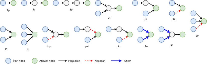
Figure 7: Query Structures used to construct queries for training RConE. Here, ‘p’, ‘i’, ‘n’, and ‘u’ are First Order Logical (FOL) operators projection, intersection, negation, and union, respectively.

TABLE III: Query generation details for each query structure.

Queries	Training		Test
Dataset	1p/2p/3p/2i/3i	2in/3in/inp/pin/pni	1p	others
FB15k	273,710	27,371	68,549	8,000
FB15k-(237)	149,689	14,698	29,962	8,000
YAGO15k	107,982	10,798	75,835	4,000
DB15k	107,982	10,798	29,799	4,000
FB15k (NMM)	273,710	27,371	67,016	8,000

Datasets and Evaluation Metrics. For evaluation, we use multi-modal datasets FB15k, FB15k-(237), YAGO15k, and DB15k [31]. We also train on FB15k (NMM) [22] (uni-modal dataset) to check whether the performance of our proposed model degrades compared to its non-multi-modal counterpart (ConE). Table II contains statistics of all the datasets. We use the average Mean Reciprocal Rank (MRR) and average HITS scores of all the answers to a query. We use these metrics for all three goals (1a, 1b, 2) described in Section IV-C.

Baselines. Since RConE is the first multi-modal logical query-answering algorithm, we choose non-multi-modal models BetaE [7] and ConE [6] as baselines. BetaE embeds the query answer distribution as $d$-dimensional beta distribution. The method was the first to handle the negation ($\neg$) operator. ConE improved on BetaE and represented the answer distribution as $d$-ary sector-cones. We cannot compare our model with path-based MMKG algorithms; hence, we omit them.

Query Generation. We propose a new query generation module that extends [7] to get both Type (I) and Type (II) answers based queries from an MMKG. The model generates FOL queries with 14 query structures (1p, 2p, 3p, 2i, 3i, pi, ip, 2u, up, pni, pin, inp, 2in, 3in) for both answer types (Figure 7). Here, p is projection, i is intersection, u is union, and n is negation. The Query generation process is divided into three modules – Scene Graph Generation, Link Prediction, and Query Traversal (figure is presented in the supplementary material).

Secondary Graph Generation. We select all the image entities from MMKG that are involved in the query generation process. The module generates a scene graph for each image using FCSGG [27]. Note that the hyper-parameters/architecture here differs from Section IV-B to keep our model independent.

Link Prediction. Each generated scene graph is connected to the original MMKG using a KG embedding algorithm, ComplEx [28]. ComplEx embeds sub-entities of all the scene graphs and the entities of MMKG into a lower-dimensional space. It then connects nodes from each scene graph to the MMKG based on the probability score. The output is a uni-modal KG.

Query Traversal. We adopt the query generation method described in [7] and incorporate Type I answers-based queries for all the 14 query structures (Figure 7) as well. Given a query structure, the algorithm chooses an answer randomly and backtracks to reach the source node while following the query structure. During traversal, it determines the relations randomly. It then executes the query again to get all the other entities that can be reached, given the source and the query.

V-B Hyper-Parameters and Model Selection

TABLE IV: Average MRR (%) score for candidate multi-modal entities (first three rows of each dataset) and answer sub-entities (grey row) for Type (I) answers. Bold results indicate the best score.

Dataset	Model	1p	2p	3p	2i	3i	pi	ip	2u	up	pni	pin	inp	2in	3in	AVG
FB15k	BetaE	5.9	1.9	0.8	6.9	8.0	5.7	1.8	5.7	1.8	4.9	0.9	0.7	5.0	5.5	4.0
	ConE	8.0	4.3	2.9	9.9	8.3	7.3	4.3	7.8	4.6	5.5	2.9	1.8	4.6	5.0	5.5
	RConE	89	40	28	92	95	67	33	85	41	74	34	19	75	72	62
	RConE(S)	72	66	56	63	64	66	75	75	68	56	59	72	65	51	65
FB15k-(237)	BetaE	29	20	10	30	33	28	15	26	17	24	7.5	6.1	19	22	20
	ConE	9.5	11	7.9	8.4	9.1	11	10	10	11	6.5	5.6	3.8	4.8	6.0	8.0
	RConE	99	65	44	99	99	92	52	99	60	91	46	24	88	91	76
	RConE(S)	77	62	59	70	71	69	71	84	64	48	58	65	57	49	65
YAGO15k	BetaE	5.8	0.9	0.9	4.5	2.3	2.0	1.3	2.9	1.1	2.0	0.8	0.8	2.2	0.8	2.0
	ConE	1.5	0.4	0.6	0.4	0.3	0.4	0.5	1.1	0.8	0.3	0.4	0.6	0.4	0.0	0.6
	RConE	86	40	24	91	73	51	32	66	30	63	23	15	67	33	54
	RConE(S)	49	47	46	54	50	44	47	49	45	44	42	44	47	44	47
DB15k	BetaE	22	12	7.7	24	24	19	13	17	12	18	11	9.4	17	18	16
	ConE	8.4	10	7.5	8.2	8.2	9.9	11	7.8	9.8	5.1	6.8	6.8	5.6	6.2	8.0
	RConE	81	34	20	92	95	73	33	79	33	78	30	20	79	88	64
	RConE(S)	44	40	42	43	44	39	40	47	41	40	40	40	39	41	41

Scene Graph Generation. We choose FCSGG [27] as a scene graph generation algorithm. The model consists of a Convolutional Neural Network for object detection and relation prediction in a single training module. The single training module results in substantial decrease in the inference time and number of parameters. This is critical, as the scene graph generation sub-module should not be a bottleneck and slow the overall training/inference of RConE. Hence, it is a preferred choice compared to other algorithms. The model uses relation affinity fields to achieve better results on unseen visual relationships and helps transfer context between the objects detected and the relations predicted.

The model implements zero-shot learning for custom image prediction and labels the entities and relations based on the training dataset. The assumption is that the training set would have enough entity and relation diversity to be useful for our dataset. We use Visual-Genome [32] for training.

The sub-module is used in both RConE and query generation. To make them independent, we use HRNet-W48[33] for query generation and HRNet-W32 for training. During training, we compare the individual sub-entities in the two generated sub-graphs above, using GloVe embeddings [34].

Scene Graph Embedding. We chose ComplEx as a translation-based model because of its relatively simpler architecture than the neural models. Like the scene graph generation sub-module, the simpler choice helps to avoid bottlenecks.

In the query generation module, we need the ComplEx algorithm to merge the scene graph generated for each multi-modal entity with the MMKG. We choose the threshold between [0, 1] to have at least one edge between the two graphs; we keep a cap of a maximum of 100 edges for each pair of graphs. The settings for the other hyper-parameters are the similar to  [28].

Query Generation. We added a constraint for query generation that the query’s source node(s) would always belong to the MMKG. For multi-modal datasets, we include a fraction of the images (5%) described in the original datasets to get a good mix of multi-modal and non-multi-modal queries. Due to computational constraints, we generated $30\%$ of training queries for which at least one answer of the query is the sub-entity. The query generation statistics for each dataset are provided in Table III.

The baselines are trained on the uni-modal queries, as the models cannot detect the sub-entities for the Type (I) answers. Moreover, these models cannot distinguish between multi-modal entities that are answers (Type (II) answers) and those containing the sub-entities as answers (Type (I) answers’ candidate entity).

To make the comparison fair for baselines, we modified the test set (for baselines) to reach the candidate multi-modal entities only as answers in the case of Type (I) answers (get only to the Toy Story (Poster) as answers, and not Green, in case of Q1). The test set for Type (II) answers is identical for RConE and the baselines.

RConE. We train our model for 200k epochs for each multi-modal dataset. $\lambda_{l1}=1$, $\lambda_{l2}=0.005$ for the loss function (Equation 31). For distance weightage ($d_{o}$, $d_{i}$, $d_{m}$), $\lambda_{1}=0.02,\lambda_{2}=1$, in the case of non-multi-modal queries, and $\lambda_{1}=0.9,\lambda_{2}=0.02$ for multi-modal queries. For the projection operator, we use $d=2400$ for the multi-modal datasets. We use one layer of transformer for training. Other configurations are the same as the ConE algorithm. Experiments are executed on NVIDIA GeForce RTX 2080 Ti GPUs.

TABLE V: Average HITS (%) score for candidate multi-modal entities (@10) (first three rows of each dataset) and answer sub-entities (@5) (grey row) for Type (I) answers. Bold results indicate the best score.

Dataset	Model	1p	2p	3p	2i	3i	pi	ip	2u	up	pni	pin	inp	2in	3in	AVG
FB15k	BetaE	12	3.9	1.4	16	18	11	3.6	12	3.2	10	1.9	1.3	10	12	8.5
	ConE	16	7.8	5.9	22	18	14	8.8	15	8.9	10	6.1	3.6	8.3	10	11
	RConE	98	64	47	99	99	87	54	93	63	95	61	37	97	93	81
	RConE(S)	92	90	84	89	90	90	93	95	91	81	84	92	88	79	88
FB15k-(237)	BetaE	53	35	21	55	57	50	27	47	29	42	15	11	37	42	37
	ConE	18	22	15	18	17	21	19	18	20	12	10	8.5	10	11	16
	RConE	99	85	65	100	100	99	74	99	78	99	71	46	99	99	89
	RConE(S)	95	87	86	93	93	90	91	97	89	78	82	88	83	75	88
YAGO15k	BetaE	11	1.5	2.0	9.7	5.4	4.8	2.6	7.3	2.1	4.7	2.0	1.5	5.1	1.7	4.4
	ConE	2.9	0.7	1.3	1.2	0.8	0.6	1.1	2.2	1.8	0.5	1.0	1.0	0.7	0.0	1.1
	RConE	93	56	38	99	86	65	49	82	45	87	37	28	90	38	71
	RConE(S)	76	76	77	85	81	72	76	79	75	74	74	75	77	76	77
DB15k	BetaE	42	24	14	44	44	39	24	33	21	35	21	17	34	35	31
	ConE	16	21	15	16	14	20	20	15	19	10	12	13	11	12	15
	RConE	93	58	37	99	99	90	55	89	54	91	51	36	91	97	80
	RConE(S)	74	70	72	73	71	67	71	80	72	71	69	69	69	71	71

TABLE VI: Average MRR (%) score for non-multi-modal query answers (Type (II) answers). Bold results indicate the best score.

Dataset	Model	1p	2p	3p	2i	3i	pi	ip	2u	up	pni	pin	inp	2in	3in	AVG
FB15k	BetaE	42	12	12	33	47	25	12	15	12	7.1	4.6	7.2	8.5	9.1	17
	ConE	68	27	22	55	67	44	30	41	24	14	8.2	11	15	15	32
	RConE	57	23	21	46	59	37	26	25	21	10	6.6	10	11	12	26
FB15k-(237)	BetaE	37	10	9.1	25	37	20	11	11	9.5	3.6	3.5	7.2	4.9	7.0	14
	ConE	42	11	10	30	43	23	14	13	10	3.9	4.4	7.6	5.6	9.0	16
	RConE	39	11	10	28	40	21	13	11	9.9	3.9	3.6	7.7	5.8	8.7	15
YAGO15k	BetaE	77	60	43	88	93	70	54	79	58	48	39	33	58	57	61
	ConE	88	76	66	96	98	79	61	94	77	64	62	46	79	72	76
	RConE	77	69	62	90	94	70	55	76	68	54	47	39	63	59	66
DB15k	BetaE	76	53	33	92	96	80	61	86	55	59	37	33	62	56	63
	ConE	85	64	47	97	98	87	67	96	71	72	54	41	78	71	73
	RConE	74	56	40	92	96	77	60	80	59	61	39	32	64	54	63

TABLE VII: Average HITS@10 (%) score for non-multi-modal query answers (Type (II) answers). Bold results indicate the best score.

Dataset	Model	1p	2p	3p	2i	3i	pi	ip	2u	up	pni	pin	inp	2in	3in	AVG
FB15k	BetaE	69	25	23	57	72	45	25	32	24	15	10	15	18	20	32
	ConE	89	44	37	78	87	65	47	61	42	28	18	23	32	33	49
	RConE	79	40	36	70	81	57	43	42	37	22	14	21	25	26	42
FB15k-(237)	BetaE	58	20	17	46	59	36	22	22	19	8.0	7.5	15	11	15	25
	ConE	62	23	19	51	65	40	25	25	20	8.5	9.8	16	12	19	28
	RConE	59	22	19	49	62	37	25	22	19	8.5	7.9	16	12	19	27
YAGO15k	BetaE	94	85	67	98	99	86	71	96	77	83	72	57	93	93	84
	ConE	97	92	83	99	99	89	76	99	87	89	84	71	97	97	90
	RConE	90	88	78	98	99	84	69	86	81	83	75	63	92	90	84
DB15k	BetaE	93	75	54	99	99	92	80	97	75	93	67	57	95	92	84
	ConE	95	83	64	99	99	95	84	99	86	96	78	68	98	96	89
	RConE	89	77	58	98	99	90	78	90	78	91	65	56	93	87	82

TABLE VIII: MRR (%) score FB15k (NMM) dataset

Model	1p	2p	3p	2i	3i	pi	ip	2u	up	pni	pin	inp	2in	3in	AVG
BetaE	64	24	24	55	66	43	27	40	24	12	6.1	11	13	14	30
ConE	73	33	28	64	73	50	35	54	31	14	9.5	12	17	18	37
RConE	73	33	29	64	72	50	34	53	31	14	9.0	12	17	18	36

V-C Discussion

[RQ1, RQ2] Logical query answers involving multi-modal entities and consisting of a sub-entity as an answer.

As discussed earlier, for an MMKG, we generate $30\%$ of queries consisting of at least one Type (I) answer and $70\%$ of queries with at least one Type (II) answer. Table IV consists of the average MRR score for all the Type (I) answers to queries on four multi-modal datasets. The table consists of two rows of results for our model, RConE and RConE (S). The RConE row consists of the average MRR score for the candidate multi-modal entities (Toy Story (Poster) in Q1), and RConE (S) (grey row) consists of the average MRR score for the answer sub-entities (Green in Q1). As the baselines cannot detect the sub-entities for Type (I) answers, we calculate the scores for the candidate multi-modal entities. This comparison aims to evaluate if the baseline models can detect even these candidate entities and if their embedding is any closer to other answers. The first three rows in Table IV show the comparison (for these candidate entities). As can be seen in the table, the RConE model performs significantly better than the baselines, with an average score improvement of $56.5$ in the case of FB15k. The MRR score decreases as we increase query complexity ($1p\rightarrow 2p\rightarrow 3p$). Though we cannot compare the sub-entity score (RConE (S)) with baselines, the values are significantly high to validate our model’s performance. Table V shows the average HITS@10 score for candidate multi-modal entities and the HITS@5 score for answer sub-entities for Type (I) answers. We choose the HITS@5 score rather than HITS@10 for the sub-entities in Table V since the number of sub-entities in a scene graph is less when compared with entities in a graph. So, it would be more competitive to present the HITS@5 score rather than 10. The HITS score shows similar trends as the MRR score.

We compare the MRR score of our model RConE for the Type (II) answers (John Lasseter in Q2). Since we train our model on both Type (I) and Type (II) answer type queries, this experiment tells the impact on the score for RConE in the case of non-multi-modal answers (in MMKGs). As we can see from Table VI, the MRR score of RConE is less than its counterpart, ConE, in most cases. However, our model performs equivalent or better than BetaE based on average (AVG) scores for all the datasets. Table VII shows the average HITS score for Type (II) answers on all the multi-modal datasets. Similar to the MRR score, the HITS score is consistently better than BetaE, except for the DB15k dataset, where the drop is not substantial.

We can expect that the baseline models will perform better in Table VI as these models are finetuned to handle only one type of query answer (Type (II) answers). In contrast, our model is more generalized and can handle both types of answers (Type (I) and Type (II)) simultaneously. RConE’s decrease in the MRR score is reasonable, as it is still performing on par or better than BetaE on average. Moreover, the decline in Table VI is much less than the significant gain RConE gets for detecting the candidate entities in Table IV. Hence, overall, our model performs better than the baseline models if we combine Table IV and VI scores in the case of MRR score (similar trends for HITS score) for an MMKG dataset.

We also performed evaluations using the non-multi-modal dataset FB15k (NMM) to check the impact of changes made to RConE with respect to the base ConE model. The MRR score is shown in Table VIII. As can be seen from the results, the performance does not drop from the original model.

V-D Fuzzy (Boundary) Region Integration Analysis

In this sub-section, we check the impact of adding the fuzzy region to the original ConE embedding. For this, we compare the neural implementation of the projection operator with the actual set operator. However, the neural method may not precisely imitate the set operator. The goal is to check the performance using the fuzzy region compared to other components and baselines. We use the model trained on the FB15k dataset.

We randomly generate $8000$ pairs of RConE embeddings $(A_{i},B_{i})$, such that $A_{i}\subseteq B_{i}$. The goal is to check if, after the projection operation, the final embeddings $A_{Pi}$ and $B_{Pi}$ are still holding the relation $A_{Pi}\subseteq B_{Pi}$. We select an arbitrary relation, $r_{i}$, from the relation set in the FB15k dataset for the projection. We check the intersection area by calculating the score as $sc=Ar(A_{Pi}\cap B_{Pi})/Ar(A_{Pi})$, where $Ar()$ is the area of the sector cone. The score for the rigid region is $41\%$, while for the fuzzy region, it is $57\%$. The score for the ConE model is $46\%$. For the actual projection operator, the rigid region slightly drops in the score if we compare it with the baseline, and the score of the fuzzy part lies in the same range (better in this case). Hence, the fuzzy region performs on par with our model’s other neural structures and baselines. Therefore, the component addition is reasonable.

V-E Time Complexity Analysis

[RQ3] Efficiency and scalability of RConE.

Efficiency. Generating scene graphs for each multi-modal entity before training, even if there is no query related to it, will incur extra overhead. To counter this, in RConE, we extract the scene graph for the multi-modal entities belonging to the fuzzy region only, which substantially decreases the computational cost.

Scalability. For the RCE module, we are adding a parameter, $\theta_{fu}$, in the original ConE architecture. Its space complexity depends on the number of relations in the MMKG, while its time complexity for each operator in RCE is on par with $\theta_{ri}$. Hence, it would not have much impact on the computation cost as we scale (compared to ConE). The Sub-Entity Prediction module uses three architectures: Scene Graph Generation, Scene Graph Embedding, and Graph Transformation. We train the Scene Graph Generation module to generate graphs to a dataset (Visual Genome) which is independent of the MMKG size. The Scene Graph embedding module’s time complexity depends on the scene graph’s size and is independent of the size of the KG. For the Graph Transformation module, we have neighbors of the multi-modal entity for external context. In real-world scale-free networks, the degree distribution follows near power law, with few nodes having a substantial number of neighbors, so it would have little impact as we scale. Hence, we can say that RConE is scalable.

VI Conclusion and Future Work

In this work, we proposed a novel method, RConE, for extracting information from multi-modal entities to resolve logical queries. Our model is the first to answer logical queries related to multi-modal entities and can handle queries with sub-entities as answers. Our proposed model can also generalize well in handling multi-modal and non-multi-modal answer based queries. It performs very efficiently for multi-modal query answers, with minimal impact on non-multi-modal answers. We also provide a novel query generation module for MMKGs, which would be helpful for the research community in generating queries with sub-entity answers.

The future goal is to explore the idea of inductive question answering and to get an answer by fusing information from multiple entities of different modalities for better context while answering a query. Apart from images, we will also consider working on other modalities for query answering.

Mayank Kharbanda received the bachelor’s and master’s degrees in computer science from the University of Delhi, India, in 2018, and 2020, respectively. He is currently working towards the PhD degree with the Department of Computer Science, IIIT Delhi. His research interests include knowledge graphs, graph representation learning and discrete mathematics. He is a UGC-JRF/SRF fellow.

Rajiv Ratn Shah Rajiv Ratn Shah is an Associate Professor in the CSE department at IIIT-Delhi. He also serves as the head of the TCS Center of Design and New Media (CDNM), and MIDAS Research Lab. Additionally, he is the director of Kyron, an edtech startup. Before joining IIIT-Delhi, he worked as a Research Fellow at the Living Analytics Research Center at Singapore Management University. More information is available at https://midas.iiitd.ac.in/.

Raghava Mutharaju is an Associate Professor in the CSE department of IIIT-Delhi, India and leads the Knowledgeable Computing and Reasoning (KRaCR) Lab. He has worked in Industry research labs such as GE Research, IBM Research, Bell Labs, and Xerox Research. His research interests include knowledge graphs, ontology modelling, reasoning, querying, and its applications. He has published at several venues, such as AAAI, ISWC, ESWC, ACL, ECML, EACL, and ECAI. More information is available at https://kracr.iiitd.edu.in/.

-A Algorithm

Algorithm 1 provides the pseudo-code for RConE. The model first initializes embeddings for all the entities and relations. It also pre-trains the scene graph generation module (Lines 1-2). For each training iteration, it selects a random query $q_{i}\in Q_{train}$ (Lines 3-4). The model picks the start nodes from the computational graph of query $q_{i}$ (Line 5). It then traverses the MMKG based on the query and executes FOL operators until it reaches the end of the computational graph (Lines 6-7). This gives $\boldsymbol{V}^{c}_{q_{i}}$ as query embedding, an answer set for Type II answers, and candidate multi-modal entities. We then calculate the loss $L_{c}$, $L_{mm}$ (Equation 31) (Line 9). The model generates a scene graph for each candidate multi-modal entity containing the answer. It then embeds the scene graph and transforms it to the query embedding space (Lines 11-13). Loss $L_{se}$ is calculated for the sub-entity answer (Equation 31) (Line 15).

-B Dataset Description

$\blacksquare$ Freebase-15k (FB15k (NMM)) [22] is a subset of the original Freebase dataset of general facts. The dataset consists of 14,951 entities and 1,345 relations. Both entities and relations have at least 100 mentions. $\blacksquare$ Freebase-15k Multi-Modal (FB15k) [31] is a multi-modal extension of the original FB15k (NMM) dataset. It consists, on average, 55.8 scaled images for each entity present in the KG. $\blacksquare$ Freebase-15k (237) Multi-Modal (FB15k-(237)) [31] is the FB15k dataset with 237 relations in it. The original non-multi-modal dataset was proposed to counter the problem of inverse relation test leakage [35]. $\blacksquare$ YAGO Multi-Modal (YAGO15k) [31] Similar to FB15k, this is a multi-modal extension of Yet Another Great Ontology (YAGO) dataset [36]. The YAGO dataset extends the information of Wordnet by merging general knowledge from Wikipedia. $\blacksquare$ DBPedia Multi-Modal (DB15k) [31] DB15k is an extension of the original DBpedia dataset [37], with images as entities included in it.

-C Query Generation

Figure 8 represents the query generation module.

-D Results

Table IX shows the average HITS@3 score for both candidate and answer sub-entities. Table X shows the average HITS@3 score for Type (II) answers on all the multi-modal datasets. The trends in both tables are similar to the HITS@10 scores presented in the main paper.

Input: MMKG-$G(\mathcal{V},\mathcal{R},\mathcal{U},\mathcal{M})$, Training Query Set-$Q_{train}$
Output: Trained model

1:  $\text{Initialize entity and relation embedding in }G\text{ as }$ $\boldsymbol{v}=(\boldsymbol{\theta}_{ax},\boldsymbol{0},\boldsymbol{0})$, $\boldsymbol{r}=(\boldsymbol{\theta}_{ax,r},\boldsymbol{\theta}_{ri,r},\boldsymbol{\theta}_{fu,r})$

2:  pre-train scene graph generation module (Section IV-B)

3:  while iterations $<$ Training iterations do

4:     $\text{Randomly select }q_{i}\in Q_{train}$

5:     $\text{Start from }\boldsymbol{v}_{start}\in q_{i}$

6:     while we reach end of computational graph do

7:        Do one of the operation from projection, intersection, negation and union over query embedding. ($\boldsymbol{V}^{c}_{q}=(\boldsymbol{\theta}_{ax},\boldsymbol{\theta}_{ri},\boldsymbol{\theta}_{fu})$) (Section IV-A)

8:     end while

9:     Calculate $L_{c}$ and $L_{mm}$ (Equation 31).

10:     for $v\in$ candidate multi-modal set do

11:        generate scene graph(v)

12:        embed scene graph(v)

13:        transform scene graph embedding (v) (Section IV-B)

14:     end for

15:     Calculate $L_{se}$ (Equation 31).

16:  end while

Algorithm 1 RConE

Appendix A Experiments

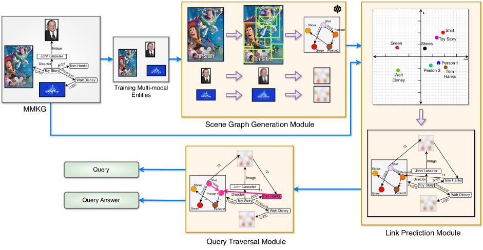
Figure 8: Query Generation: The Scene Graph Generation module takes all the image entities from the Multi-Modal Knowledge Graph (MMKG) as input and generates a scene graph for each entity. Link Prediction Module predicts links between these scene graphs and the original MMKG. Query Traversal Module generates queries for multiple query structures based on the entire knowledge graph (actual MMKG and scene graphs merged).

TABLE IX: Average HITS@3 (%) score for candidate multi-modal entities (first three rows of each dataset) and answer sub-entities (grey row) for Type (I) answers. Bold results indicate the best score.

Dataset	Model	1p	2p	3p	2i	3i	pi	ip	2u	up	pni	pin	inp	2in	3in	AVG
FB15k	BetaE	5.6	1.7	0.4	7.0	7.8	5.7	1.7	5.8	1.7	4.3	0.5	0.3	4.3	4.6	3.7
	ConE	8.8	4.1	2.3	11	8.7	7.7	4.3	8.2	4.8	5.4	2.7	1.7	4.6	5.3	5.7
	RConE	93	45	30	96	97	74	36	87	44	83	39	20	88	80	67
	RConE(S)	83	79	67	77	76	77	84	87	79	66	69	82	76	61	76
FB15k-(237)	BetaE	34	23	11	36	37	33	16	30	19	27	7.8	6.5	21	24	23
	ConE	10	11	8.0	8.4	9.4	12	11	10	11	6.5	5.5	3.6	4.7	6.1	8.0
	RConE	99	72	48	99	99	96	58	99	66	97	53	27	98	97	80
	RConE(S)	88	73	71	83	83	80	81	92	75	58	68	76	68	58	75
YAGO15k	BetaE	5.6	0.5	0.8	4.5	1.7	1.7	1.0	1.9	0.8	1.6	0.5	0.7	1.6	0.6	1.7
	ConE	1.3	0.2	0.7	0.2	0.3	0.2	0.2	0.8	0.7	0.1	0.1	0.4	0.2	0.0	0.4
	RConE	89	43	25	96	79	55	34	70	32	73	25	16	78	54	59
	RConE(S)	59	56	58	67	61	53	57	60	55	54	51	53	59	55	57
DB15k	BetaE	24	14	7.6	27	27	21	14	18	13	20	12	10	19	19	18
	ConE	9.4	12	8.4	8.7	9.1	11	12	8.5	10	5.6	7.9	7.7	6.0	7.1	8.9
	RConE	86	39	22	96	98	81	37	82	37	83	34	21	84	93	69
	RConE(S)	53	49	51	52	53	47	49	59	50	48	46	47	47	49	50

TABLE X: Average HITS@3 (%) score for non-multi-modal query answers (Type (II) answers). Bold results indicate the best score.

Dataset	Model	1p	2p	3p	2i	3i	pi	ip	2u	up	pni	pin	inp	2in	3in	AVG
FB15k	BetaE	47	13	12	38	53	28	13	16	12	6.4	3.7	6.7	7.7	8.6	19
	ConE	77	29	24	63	75	49	32	46	27	14	7.4	11	16	16	35
	RConE	64	25	23	52	65	41	28	28	23	10	5.8	10	11	11	28
FB15k-(237)	BetaE	41	10	9.0	28	42	22	12	11	9.6	2.7	2.4	6.5	4.0	6.2	15
	ConE	46	12	10	34	49	26	15	13	11	3.0	3.5	7.5	4.6	8.3	17
	RConE	43	11	10	32	45	23	14	12	10	3.2	2.8	7.2	5.2	8.1	16
YAGO15k	BetaE	84	66	48	94	97	75	59	87	63	63	50	37	77	75	70
	ConE	92	82	71	98	99	82	65	97	81	74	70	52	90	87	81
	RConE	80	75	66	94	97	74	58	79	72	65	56	43	77	73	72
DB15k	BetaE	83	59	36	96	98	85	67	92	60	80	45	37	83	75	71
	ConE	89	70	50	98	99	91	73	98	76	87	62	47	92	86	80
	RConE	80	62	44	95	98	83	64	84	64	76	46	36	80	67	70

References

- [1] A. Hogan, E. Blomqvist, M. Cochez, C. d’Amato, G. D. Melo, C. Gutierrez, S. Kirrane, J. E. L. Gayo, R. Navigli, S. Neumaier et al., “Knowledge graphs,” ACM Computing Surveys (Csur), vol. 54, no. 4, pp. 1–37, 2021.
- [2] S. Ji, S. Pan, E. Cambria, P. Marttinen, and S. Y. Philip, “A survey on knowledge graphs: Representation, acquisition, and applications,” IEEE transactions on neural networks and learning systems, vol. 33, no. 2, pp. 494–514, 2021.
- [3] J. Zhang, B. Chen, L. Zhang, X. Ke, and H. Ding, “Neural, symbolic and neural-symbolic reasoning on knowledge graphs,” AI Open, vol. 2, pp. 14–35, 2021.
- [4] H. Ren, W. Hu, and J. Leskovec, “Query2box: Reasoning over knowledge graphs in vector space using box embeddings,” arXiv preprint arXiv:2002.05969, 2020.
- [5] H. Ren, M. Galkin, M. Cochez, Z. Zhu, and J. Leskovec, “Neural graph reasoning: Complex logical query answering meets graph databases,” arXiv preprint arXiv:2303.14617, 2023.
- [6] Z. Zhang, J. Wang, J. Chen, S. Ji, and F. Wu, “Cone: Cone embeddings for multi-hop reasoning over knowledge graphs,” Advances in Neural Information Processing Systems, vol. 34, pp. 19 172–19 183, 2021.
- [7] H. Ren and J. Leskovec, “Beta embeddings for multi-hop logical reasoning in knowledge graphs,” Advances in Neural Information Processing Systems, vol. 33, pp. 19 716–19 726, 2020.
- [8] X. Zhu, Z. Li, X. Wang, X. Jiang, P. Sun, X. Wang, Y. Xiao, and N. J. Yuan, “Multi-modal knowledge graph construction and application: A survey,” IEEE Transactions on Knowledge and Data Engineering, 2022.
- [9] W. Xiong, T. Hoang, and W. Y. Wang, “Deeppath: A reinforcement learning method for knowledge graph reasoning,” arXiv preprint arXiv:1707.06690, 2017.
- [10] X. V. Lin, C. Xiong, and R. Socher, “Multi-hop knowledge graph reasoning with reward shaping,” Apr. 18 2023, uS Patent 11,631,009.
- [11] X. Chen, M. Chen, W. Shi, Y. Sun, and C. Zaniolo, “Embedding uncertain knowledge graphs,” in Proceedings of the AAAI conference on artificial intelligence, vol. 33, no. 01, 2019, pp. 3363–3370.
- [12] S. Guo, Q. Wang, L. Wang, B. Wang, and L. Guo, “Knowledge graph embedding with iterative guidance from soft rules,” in Proceedings of the AAAI Conference on Artificial Intelligence, vol. 32, no. 1, 2018.
- [13] S. Guo, Q. Wang, L. Wang, B. Wang, and L. Guo, “Jointly embedding knowledge graphs and logical rules,” in Proceedings of the 2016 conference on empirical methods in natural language processing, 2016, pp. 192–202.
- [14] H. Wang, H. Ren, and J. Leskovec, “Entity context and relational paths for knowledge graph completion,” arXiv preprint arXiv:2002.06757, p. 47, 2020.
- [15] W. Hamilton, P. Bajaj, M. Zitnik, D. Jurafsky, and J. Leskovec, “Embedding logical queries on knowledge graphs,” Advances in neural information processing systems, vol. 31, 2018.
- [16] D. Alivanistos, M. Berrendorf, M. Cochez, and M. Galkin, “Query embedding on hyper-relational knowledge graphs,” arXiv preprint arXiv:2106.08166, 2021.
- [17] H. Luo, Y. Yang, G. Zhou, Y. Guo, T. Yao, Z. Tang, X. Lin, K. Wan et al., “Nqe: N-ary query embedding for complex query answering over hyper-relational knowledge graphs,” arXiv preprint arXiv:2211.13469, 2022.
- [18] X. Lin, C. Xu, F. Su, G. Zhou, T. Hu, N. Li, M. Sun, H. Luo et al., “Tflex: Temporal feature-logic embedding framework for complex reasoning over temporal knowledge graph,” arXiv preprint arXiv:2205.14307, 2022.
- [19] K. Liang, L. Meng, M. Liu, Y. Liu, W. Tu, S. Wang, S. Zhou, X. Liu, and F. Sun, “A survey of knowledge graph reasoning on graph types: Static, dynamic, and multimodal,” 2022.
- [20] R. Xie, Z. Liu, H. Luan, and M. Sun, “Image-embodied knowledge representation learning,” arXiv preprint arXiv:1609.07028, 2016.
- [21] Z. Wang, L. Li, Q. Li, and D. Zeng, “Multimodal data enhanced representation learning for knowledge graphs,” in 2019 International Joint Conference on Neural Networks (IJCNN). IEEE, 2019, pp. 1–8.
- [22] A. Bordes, N. Usunier, A. Garcia-Duran, J. Weston, and O. Yakhnenko, “Translating embeddings for modeling multi-relational data,” Advances in neural information processing systems, vol. 26, 2013.
- [23] S. Zheng, W. Wang, J. Qu, H. Yin, W. Chen, and L. Zhao, “Mmkgr: Multi-hop multi-modal knowledge graph reasoning,” arXiv preprint arXiv:2209.01416, 2022.
- [24] S. P. Boyd and L. Vandenberghe, Convex optimization. Cambridge university press, 2004.
- [25] Z. Liao and J. Zhou, “Rough convex cones and rough convex fuzzy cones,” Soft Computing, vol. 16, pp. 2083–2087, 2012.
- [26] Z. Pawlak, “Rough sets,” International journal of computer & information sciences, vol. 11, pp. 341–356, 1982.
- [27] H. Liu, N. Yan, M. Mortazavi, and B. Bhanu, “Fully convolutional scene graph generation,” in Proceedings of the IEEE/CVF Conference on Computer Vision and Pattern Recognition, 2021, pp. 11 546–11 556.
- [28] T. Trouillon, J. Welbl, S. Riedel, É. Gaussier, and G. Bouchard, “Complex embeddings for simple link prediction,” in International conference on machine learning. PMLR, 2016, pp. 2071–2080.
- [29] A. Vaswani, N. Shazeer, N. Parmar, J. Uszkoreit, L. Jones, A. N. Gomez, Ł. Kaiser, and I. Polosukhin, “Attention is all you need,” Advances in neural information processing systems, vol. 30, 2017.
- [30] W. Hamilton, Z. Ying, and J. Leskovec, “Inductive representation learning on large graphs,” Advances in neural information processing systems, vol. 30, 2017.
- [31] Y. Liu, H. Li, A. Garcia-Duran, M. Niepert, D. Onoro-Rubio, and D. S. Rosenblum, “Mmkg: multi-modal knowledge graphs,” in The Semantic Web: 16th International Conference, ESWC 2019, Portorož, Slovenia, June 2–6, 2019, Proceedings 16. Springer, 2019, pp. 459–474.
- [32] R. Krishna, Y. Zhu, O. Groth, J. Johnson, K. Hata, J. Kravitz, S. Chen, Y. Kalantidis, L.-J. Li, D. A. Shamma et al., “Visual genome: Connecting language and vision using crowdsourced dense image annotations,” International journal of computer vision, vol. 123, pp. 32–73, 2017.
- [33] J. Wang, K. Sun, T. Cheng, B. Jiang, C. Deng, Y. Zhao, D. Liu, Y. Mu, M. Tan, X. Wang et al., “Deep high-resolution representation learning for visual recognition,” IEEE transactions on pattern analysis and machine intelligence, vol. 43, no. 10, pp. 3349–3364, 2020.
- [34] J. Pennington, R. Socher, and C. D. Manning, “Glove: Global vectors for word representation,” in Proceedings of the 2014 conference on empirical methods in natural language processing (EMNLP), 2014, pp. 1532–1543.
- [35] K. Toutanova, D. Chen, P. Pantel, H. Poon, P. Choudhury, and M. Gamon, “Representing text for joint embedding of text and knowledge bases,” in Proceedings of the 2015 conference on empirical methods in natural language processing, 2015, pp. 1499–1509.
- [36] M. Fabian, K. Gjergji, W. Gerhard et al., “Yago: A core of semantic knowledge unifying wordnet and wikipedia,” in 16th International world wide web conference, WWW, 2007, pp. 697–706.
- [37] S. Auer, C. Bizer, G. Kobilarov, J. Lehmann, R. Cyganiak, and Z. Ives, “Dbpedia: A nucleus for a web of open data,” in international semantic web conference. Springer, 2007, pp. 722–735.