Brownian and fractional polymers with self-repulsion

Abstract

Brownian and fractional processes are useful computational tools for the modelling of physical phenomena. Here, modelling linear homopolymers in solution as Brownian or fractional processes, we develop a formalism to take into account both the interactions of the polymer with the solvent as well as the effect of arbitrary polymer-polymer potentials and Gibbs factors. As an example the average squared length is computed for a non-trivial Gaussian Gibbs factor, which is also compared with the Edwards’ and a step factor.

1 Brownian and fractional processes as a modelling and computational tool

From its discovery in the nineteen century [1] to a model for financial market fluctuations [2], to a clear evidence for the existence of atoms [3] and the inclusion in a more general class of Lévy processes, Brownian motion has played a central role in the modelling of physical phenomena and, in mathematics, in the development of the field of stochastic and infinite-dimensional analysis [4]. Brownian motion has independent increments, but is a particular case of fractional Gaussian processes which, being either positively or negatively correlated, allow for the modelling of memory effects .

Brownian motion, and more general Gaussian processes, are also an useful tool even in non-stochastic contexts. New solutions for deterministic nonlinear partial differential equations may be obtained by a stochastic construction, based on diffusion plus branching processes. This has been used, for example, for the Navier-Stokes equation [5] [6], for magnetohydrodynamics [7], for fractional [8] and singular partial differential equations [9], etc.

Here we address the problem of modelling of polymers in solvents. The behavior of polymers in solvents is determined by their chemical structures. Very diverse patterns are observed. If, in a few instances, polymer molecules display little interaction with the solvent, in most cases they either curl up on itself or stretch out. A widely used characterization of the polymer behavior is the Flory-Huggins parameter $\chi$ [11] [12] which, based on the entropy of mixing, attempts to take into account both the interaction of the polymer chains with the solvent molecules and the polymer-polymer interaction. When the polymer is modeled by a Gaussian process, the persistent nature of the fractional processes for $H>0.5$ and anti-persistent for $H<0.5$, allows the Hurst coefficient $H$ to code for the polymer-solvent interaction, leaving the polymer-polymer interaction to be modelled by diverse interaction potentials or Gibbs factors.

The plan of the paper is the following: In Section 2 and 3, the polymer is modelled as a Gaussian (Brownian, $H=0.5$ or fractional, $H\neq 0.5$) process, each monomer being identified as a unit of ”time” in the process. Polymer-polymer interactions are taken into account by a potential $\Phi$ and its associated Gibbs factor. A general formula is obtained (Eqs.14 and 15) to compute the average squared length for arbitrary potentials through weighed integrals over Gaussian measures. Other physical polymer variables may be obtained in a similar manner.

In Section 4 we discuss several types of potentials (and Gibbs factors), in particular a potential that leads to a non-trivial Gaussian Gibbs factor and a step factor. They are compared with the Edwards’ factor [10], which turns out to be identical to the step factor. For one of the Gibbs factors, the one corresponding to the potential in Eq.(19), an exact analytical result is obtained for the average squared length (Eq.26). The average squared length $\mathbb{E}\left[x^{2}\left(L\right)\right]$ is then computed over an extensive range of Hurst parameter values $H$ and potential ranges (Fig.3). The main conclusions are:

- $\mathbb{E}\left[x^{2}\left(L\right)\right]$ converges rapidly to a power law in $L$, Fig.2.

- The scaling index $\nu$ in $\sqrt{\mathbb{E}\left[x^{2}\left(L\right)\right]}\sim L^{\nu}$, growths with $H$ and has an appreciable dependence on the potential range.

- The Flory [13] value for $\nu$ at $H=0.5$, obtained by scaling arguments, roughly corresponds to a potential range of one monomer.

2 Polymers in solvents as Gaussian processes

Polymers are long chains of molecules (monomers) connected to each other at points which allow for spatial rotations. Insofar as these rotations are relatively unconstrained, polymers may be modelled by random walks or, in the continuum limit, by paths of stochastic processes. However such models should take into account the fact that, if two chain elements come close together, molecular forces prevent them from occupying the same place. Self-crossings of paths should be suppressed and this ”excluded volume” effect explicitly taken into account. On the other hand, swelling or shrinking of the polymer chains depends on the nature of the solvent. This suggests, for stochastic polymer models, the inclusion of both excluded volume interactions and fractionality on the paths to model long range correlations.

In the continuum version of the models, both in the Brownian and the fractional Brownian cases, expectations are taken in the white noise measure [14] [15], defined by

$$\int_{S^{\prime}\left(R^{n}\right)}\exp i\left(\omega,f\right)d\mu\left(\omega\right)=\exp\left(-\frac{1}{2}\left\|f\right\|_{L^{2}\left(R^{n}\right)}^{2}\right)\hskip 28.45274ptf\in S\left(R^{n}\right),$$ (1)

Brownian motion being

$$B\left(t\right)=\left\langle\omega|\chi_{\left[0,t\right]}\right\rangle$$ (2)

with

$$\chi_{\left[0,t\right]}\left(s\right)=\left\{\begin{array}[]{ccc}1&&\text{if }0\leq s\leq t\\ 0&&\text{otherwise}\end{array}\right.$$ (3)

and fractional Brownian motion

$$B^{H}\left(t\right)=\left\langle\omega|M_{\left[0,t\right]}^{(H)}\right\rangle=\int_{0}^{t}M_{\left[0,t\right]}^{(H)}\left(s\right)d\omega\left(s\right)$$ (4)

where here, for computational convenience, we use the Molchan representation via the Wiener process on a finite time interval [16] [17]

$$M_{t}^{(H)}\left(s\right)\equiv M_{\left[0,t\right]}^{(H)}\left(s\right)=c_{H}\left\{\left(\frac{t}{s}\right)^{H-\frac{1}{2}}\left(t-s\right)^{H-\frac{1}{2}}-\left(H-\frac{1}{2}\right)s^{\frac{1}{2}-H}\int_{s}^{t}u^{H-\frac{3}{2}}\left(u-s\right)^{H-\frac{1}{2}}du\right\}$$ (5)

and

$$c_{H}=\left(\frac{2H\Gamma\left(\frac{3}{2}-H\right)}{\Gamma\left(H+\frac{1}{2}\right)\Gamma\left(2-2H\right)}\right)^{\frac{1}{2}}$$ (6)

In the continuum model, to mimic the excluded volume effect, Gibbs factors are included in the path integral. In the Edwards model, for example, the factor is

$$G=\frac{1}{Z}\exp\left(-g\int_{0}^{L}dt\int_{0}^{t}ds\delta\left(\left|B^{H}\left(t\right)-B^{H}\left(s\right)\right|\right)\right)$$ (7)

with $H=\frac{1}{2}$ in the original Edwards model [10] and $H\neq\frac{1}{2}$ in the fractional generalizations [18]. The Gibbs factor $G$ means that the excluded volume effect is controlled by the self-intersection local time $\mathcal{L}$ of the process,

$$\mathcal{L}=\int_{0}^{L}dt\int_{0}^{t}ds\delta\left(\left|B^{H}\left(t\right)-B^{H}\left(s\right)\right|\right).$$ (8)

Conceptually, this is an elegant model. However, due to the nature of $\mathcal{L}$, the physical interpretation of the Gibbs factor in (7) is rather delicate. When the $\delta$ distribution in (8) is approximated by a sequence of functions, for example

$$\delta_{\varepsilon}\left(x\right) = \frac{1}{\left(2\pi\varepsilon\right)^{n/2}}e^{-\frac{x^{2}}{2\varepsilon}};\;x\in\mathbb{R}^{n};\;\varepsilon>0,$$

$$\mathcal{L}_{\varepsilon} = \int_{0}^{L}dt\int_{0}^{t}ds\delta_{\varepsilon}\left(\left|B^{H}\left(t\right)-B^{H}\left(s\right)\right|\right),$$ (9)

one finds out that for $H=\frac{1}{2}$, $\mathcal{L}_{\varepsilon}$ converges in $L^{2}$ only for $n=1$, $n$ being the spatial dimension of the space. For $n=2$ an infinite quantity must be subtracted, centering the distribution [19]

$$\mathcal{L}_{\varepsilon,c}=\mathcal{L}_{\varepsilon}-\mathbb{E}\left(\mathcal{L}_{\varepsilon}\right).$$

In $n=2$ this is sufficient to ensure convergence of (9) when $\varepsilon\searrow 0$. For $n\geq 3$ a further multiplicative factor is needed to yield a (in law) limiting process [20] [21]. For the fractional case similar renormalization procedures have been found [18] [22] [23] [24].

All this gave rise to some pieces of beautiful mathematics but, as far as polymer physics is concerned, the model only considers the polymers as paths without transversal dimensions (which they have) and the molecular repellency as a pointwise intersection without any particular information on the molecular potential. In addition, the need for renormalization procedures or subtraction of divergent quantities, removes any relation of the results to the original coupling constants of the model.

Pointwise self interaction neglects effects of polymer structure on the physical properties and complex functions [25] of the polymers. This suggests that some other Gibbs factors, that also punish self-intersection, might be used to obtain results which take in account the polymer physical dimensions and, at the same time, rigorously relate the results to the parameters in the model. In this paper an attempt is made in this direction by developing a general analytical framework for the exploration of arbitrary interaction potentials. As an example, the average squared length is computed for a non-trivial Gaussian Gibbs factor, which is also compared with the Edwards and step Gibbs factors.

3 The average squared length

Here, as in the Edwards model, the underlying probability space is continuous white noise. However, for the calculation of expectation values, a discrete time sampling of the path will be used. For polymers, a discrete time sampling formulation is appropriate, each time step corresponding to a monomer. Then, all expectations in a linear $L-$monomers homopolymer chain will be obtained from measures

$$d\nu\left(\omega\right)=\frac{1}{Z}d\mu\left(\omega\right)\prod_{\alpha^{\prime}>\alpha\geq 1}^{L}e^{-\Phi\left(\left|\left\langle\omega|M_{\alpha}^{(H)}\right\rangle-\left\langle\omega|M_{\alpha^{\prime}}^{(H)}\right\rangle\right|\right)}$$ (10)

where $\Phi\left(\left|\left\langle\omega|M_{\alpha}^{(H)}\right\rangle-\left\langle\omega|M_{\alpha^{\prime}}^{(H)}\right\rangle\right|\right)$ is the excluded volume potential associated to interaction of the pair $\alpha,\alpha^{\prime}$ of polymer segments. For the Brownian ($H=\frac{1}{2}$) case $M_{\alpha}^{(H)}$ is the characteristic function (3) of the interval $\left[0,\alpha\right]$ and for the fractional case the integration kernel (5-6) discussed in the introduction. $\omega=\left\{\omega_{\alpha}\right\}$ is $n-$dimensional white noise and $\mu\left(\omega\right)$ the white noise Gaussian measure. The Gibbs factors should take into account all the $M=\frac{L(L-1)}{2}$ ordered $\left(\alpha,\alpha^{\prime}\right)$ pairs interactions. The partition function $Z$ is

$$Z=\int_{S^{\prime n}}d\mu\left(\omega\right)\prod_{\alpha^{\prime}>\alpha\geq 1}^{L}e^{-\Phi\left(\left|\left\langle\omega|M_{\alpha}^{(H)}\right\rangle-\left\langle\omega|M_{\alpha^{\prime}}^{(H)}\right\rangle\right|\right)}.$$ (11)

and the average squared length

$$\mathbb{E}\left[x^{2}\left(L\right)\right] = \frac{1}{Z}\int_{S^{\prime n}}d\mu\left(\omega\right)\left|\left\langle\omega|M_{L}^{(H)}\right\rangle\right|^{2}\prod_{\alpha^{\prime}>\alpha\geq 1}^{L}e^{-\Phi\left(\left|\left\langle\omega|M_{\alpha}^{(H)}\right\rangle-\left\langle\omega|M_{\alpha^{\prime}}^{(H)}\right\rangle\right|\right)}$$

with lengths defined in the $\mathbb{R}^{n}$ Euclidean metric and integration of the Wiener process with the kernels $M_{\alpha}^{(H)}$. At each evolution step in (LABEL:2.3) replace $\omega$ by the operator $\frac{1}{i}\frac{\partial}{\partial\overrightarrow{J}}$ acting on $\exp i\left(\omega,\overrightarrow{J}\right)|_{\overrightarrow{J}=0}$. $\overrightarrow{J}$ is a $nL-$dimensional vector function with components in $S\left(R^{n}\right)$. Then, integrating over the $S^{\prime}\left(R^{n}\right)$ white noise measure for each one of the $L$ evolution steps, one obtains

$$\mathbb{E}\left[x^{2}\left(L\right)\right] = \frac{1}{Z}\left|\left\langle\frac{1}{i}\frac{\partial}{\partial\overrightarrow{J}}|M_{L}^{(H)}\right\rangle\right|^{2}$$

$$\left.\exp\left\{-\Phi\left(\left|\left\langle\frac{1}{i}\frac{\partial}{\partial\overrightarrow{J}}|M_{\alpha}^{(H)}\right\rangle-\left\langle\frac{1}{i}\frac{\partial}{\partial\overrightarrow{J}}|M_{\alpha^{\prime}}^{(H)}\right\rangle\right|\right)\right\}\exp\left\{-\frac{1}{2}\left\|\overrightarrow{J}\right\|^{2}\right\}\right|_{\overrightarrow{J}=0}.$$

Now one uses

$$\left.f\left(\frac{1}{i}\frac{\partial}{\partial\overrightarrow{J}}\right)e^{-\frac{1}{2}\left\|\overrightarrow{J}\right\|_{n}^{2}}\right|_{\overrightarrow{J}=0}=\left(2\pi\right)^{-\frac{n}{2}}\int d^{n}\overrightarrow{y}_{\alpha}f\left(\overrightarrow{y}_{\alpha}\right)e^{-\frac{1}{2}\left\|\overrightarrow{y}_{\alpha}\right\|^{2}}$$ (13)

to obtain

$$\mathbb{E}\left[x^{2}\left(L\right)\right]=\frac{1}{Z}\int\left(\prod_{\alpha=1}^{L}d^{n}y_{\alpha}e^{-\frac{1}{2}\sum_{\alpha}\left|\overrightarrow{y}_{\alpha}\right|^{2}}\right)\left|\left\langle\overrightarrow{y}_{L}|M_{L}^{(H)}\right\rangle\right|^{2}\prod_{\alpha^{\prime}>\alpha\geq 1}^{L}e^{-\Phi\left(\left|\left\langle\overrightarrow{y}_{\alpha}|M_{\alpha}^{(H)}\right\rangle-\left\langle\overrightarrow{y}_{\alpha^{\prime}}|M_{\alpha^{\prime}}^{(H)}\right\rangle\right|\right)}$$ (14)

and

$$Z=\int\left(\prod_{\alpha=1}^{L}d^{n}y_{\alpha}e^{-\frac{1}{2}\sum_{\alpha}\left|\overrightarrow{y}_{\alpha}\right|^{2}}\right)\prod_{\alpha^{\prime}>\alpha\geq 1}^{L}e^{-\Phi\left(\left|\left\langle\overrightarrow{y}_{\alpha}|M_{\alpha}^{(H)}\right\rangle-\left\langle\overrightarrow{y}_{\alpha^{\prime}}|M_{\alpha^{\prime}}^{(H)}\right\rangle\right|\right)}$$ (15)

where $2\pi$ powers are discarded both in $\mathbb{E}\left[x^{2}\left(L\right)\right]$ and $Z$.

At this point and before using Eqs.(14) and (15) for calculations with diverse Gibbs factors, it is useful to ponder the meaning of the replacement of the process $\omega$ in (LABEL:2.3) and (11) by an integration over a Gaussian probability density in (14) and (15) and the use of an integration variable $\overrightarrow{y}_{\alpha}$ for each evolution step.

When computing physical quantities, the Gibbs potential assigns a weight that is a function of the variable $\left|\left\langle\omega|M_{\alpha}^{(H)}\right\rangle-\left\langle\omega|M_{\alpha^{\prime}}^{(H)}\right\rangle\right|$, that is, the separation of the process at the ”times” $\alpha$ and $\alpha^{\prime}$. For a fractional process in dimension $n$, with Hurst coefficient $H$, the probability $\rho\left(\overrightarrow{z}\right)$ for a separation $\overrightarrow{z}$ after $\left|\alpha-\alpha^{\prime}\right|$  evolution steps is

$$\rho\left(\overrightarrow{z}\right)=\left(\frac{1}{2\pi n\left|\alpha-\alpha^{\prime}\right|^{2H}}\right)^{\frac{n}{2}}\exp\left(-\frac{1}{2}\frac{\left|\overrightarrow{z}\right|}{n\left|\alpha-\alpha^{\prime}\right|^{2H}}\right)$$ (16)

the covariance being $n\left|\alpha-\alpha^{\prime}\right|^{2H}$. Examination of (13) - (15) and a change of variables

$$\overrightarrow{y}=\frac{\overrightarrow{z}}{\sqrt{n}\left|\alpha-\alpha^{\prime}\right|^{H}}$$

shows that what is being done is an integration on the separation probabilities $\rho\left(\overrightarrow{z}\right)$.

4 Gibbs factors

Having taken explicit account of the relevant stochastic processes, Eqs.(14) and (15) are appropriate tools to explore, analytically or numerically, the effect of several types of polymer self-interactions corresponding to any type of interaction potential. The Edwards Gibbs factor used in the past to obtain, modulo renormalization procedures, some results for Brownian and fractional polymers (see [18],[24] and references therein) was

$$e^{-\phi_{Edwards}\left(x\right)}=e^{-g\delta\left(\left|x\right|\right)}$$ (17)

Actually, the excluding volume effect of the Edwards’ factor is very similar to the one of a step factor

$$e^{-\phi_{step}\left(x\right)}=\theta\left(\left|x\right|-\varepsilon\right).$$ (18)

This is easily seen, for example, by approximating the delta distribution by a sequence of rectangular functions of constant area and computing the Fourier transform

$$\widehat{f}_{Edwards}\left(q\right)=\left(2\pi\right)^{\frac{n}{2}}\delta^{n}\left(q\right)-\lim_{\varepsilon\rightarrow 0}\frac{1}{\left|q\right|^{\frac{n-2}{2}}}\int_{0}^{\varepsilon}r^{\frac{n}{2}}J_{\frac{n-2}{2}}\left(\left|q\right|r\right)dr\left(1-e^{-\frac{g}{\varepsilon}}\right).$$

For the step Gibbs factor the Fourier transform would be

$$\widehat{f}_{step}\left(q\right)=\left(2\pi\right)^{\frac{n}{2}}\delta^{n}\left(q\right)-\lim_{\varepsilon\rightarrow 0}\frac{1}{\left|q\right|^{\frac{n-2}{2}}}\int_{0}^{\varepsilon}r^{\frac{n}{2}}J_{\frac{n-2}{2}}\left(\left|q\right|r\right)dr$$

the conclusion being that for small $\varepsilon$ the Edwards’ Gibbs factor is identical to a step factor and the coupling constant $g$ becomes an irrelevant parameter. This is an useful fact, because it is much simpler to do practical calculations with the step factor than to handle the self-intersection local time (8).

Another Gibbs factor for which explicit analytic results, without renormalization procedures, are obtained, corresponds to the potential

$$\phi_{\beta}\left(\left|x\right|\right)=\log\frac{1}{1-\exp\left(-\beta^{2}\left|x\right|^{2}\right)}$$ (19)

with an associated Gibbs factor

$$e^{-\phi_{\beta}\left(\left|x\right|\right)}=1-\exp\left(-\beta^{2}\left|x\right|^{2}\right)$$ (20)

Fig.1 displays the potential and the Gibbs factor for several values of $\beta$ ($\beta=1,3,10$). Like the Edwards’s factor, this one also extracts from the integration domain all the $\left|x\right|=0$ hyperplanes, that is, all hyperplanes corresponding to polymer intersections but, depending on the parameter $\beta$, it also allows for repulsion at non-zero distances.

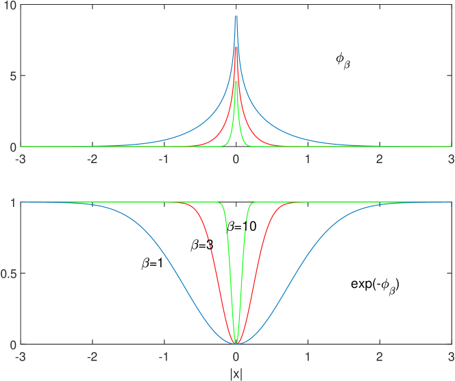
Figure 1: Potential $\phi$ and Gibbs factor $\exp\left(-\phi\right)$ for several values of $\beta$ ($\beta=1,3,10$)

The Fourier transform of this Gibbs factor is

$$\widehat{f}\left(q\right)=\left(2\pi\right)^{\frac{n}{2}}\delta^{n}\left(q\right)-\frac{1}{\left(2\beta^{2}\right)^{\frac{n}{2}}}\exp\left(-\frac{\left|q\right|^{2}}{4\beta^{2}}\right)$$ (21)

For comparison with the step (or Edwards’) factors one may compute the amount $\gamma$ of integration volume of a sphere of radius $R$ that is excluded by these factors,

$$\gamma=\frac{1}{V_{n}\left(R\right)}\int_{S\left(R\right)}e^{-\phi}d^{n}x.$$

For the step factor, identical to Edwards’ for small $\varepsilon$, it is

$$\gamma\left(\varepsilon\right)=1-\left(\frac{\varepsilon}{R}\right)^{n}$$

and for the Gaussian factor (for large $R$)

$$\gamma\left(\beta\right)\simeq 1-\frac{\Gamma\left(\frac{n}{2}+1\right)}{\left(R\beta\right)^{n}}.$$

Therefore one expects qualitatively similar effects, at large $\beta$ (small $\varepsilon$), if $\beta\sim\frac{1}{\varepsilon}$.

4.1 The Gaussian factor

$$\mathbb{E}\left[x^{2}\left(L\right)\right]_{G}=\frac{1}{Z}\int\left(\prod_{\alpha=1}^{L}d^{n}y_{\alpha}e^{-\frac{1}{2}\sum_{\alpha}\left|\overrightarrow{y}_{\alpha}\right|^{2}}\right)\left|\left\langle\overrightarrow{y}|M_{L}^{(H)}\right\rangle\right|^{2}\prod_{\alpha^{\prime}>\alpha\geq 1}^{L}\left(1-e^{-\beta^{2}\left|\left\langle y|M_{\alpha}^{(H)}\right\rangle-\left\langle y|M_{\alpha^{\prime}}^{(H)}\right\rangle\right|^{2}}\right)$$ (22)

$$Z=\int\left(\prod_{\alpha=1}^{L}d^{n}y_{\alpha}e^{-\frac{1}{2}\sum_{\alpha}\left|\overrightarrow{y}_{\alpha}\right|^{2}}\right)\prod_{\alpha^{\prime}>\alpha\geq 1}^{L}\left(1-e^{-\beta^{2}\left|\left\langle y|M_{\alpha}^{(H)}\right\rangle-\left\langle y|M_{\alpha^{\prime}}^{(H)}\right\rangle\right|^{2}}\right)$$ (23)

In the Gibbs factor the contribution corresponding to an interaction between the evolution steps $\alpha$ and $\alpha^{\prime}$ is

$$1-\exp\left(-\beta^{2}\left|\left\langle y|M_{\alpha}^{(H)}\right\rangle-\left\langle y|M_{\alpha^{\prime}}^{(H)}\right\rangle\right|^{2}\right)$$

$$= 1-\exp\left(-\beta^{2}\left|\sum_{i=1}^{\alpha}\overrightarrow{y}\left(i\right)M_{\alpha}^{(H)}\left(i\right)-\sum_{i=1}^{\alpha^{\prime}}\overrightarrow{y}\left(i\right)M_{\alpha^{\prime}}^{(H)}\left(i\right)\right|^{2}\right)$$

In the expressions above $y$ is a $nL-$dimensional vector and $M_{\alpha}^{(H)}$ a $\alpha-$dimensional one (or a $L-$dimensional vector, where only the first $\alpha$ elements are nonzero). $M_{\alpha}^{(H)}\left(i\right)$ and $M_{\alpha^{\prime}}^{(H)}\left(i\right)$ are discretized versions of the integration kernel, computed at the middle point of each interval

$$M_{\alpha}^{(H)}\left(i\right)=c_{H}\left\{\left(\frac{\alpha}{i-\frac{1}{2}}\right)^{H-\frac{1}{2}}\left(\alpha-i-\frac{1}{2}\right)^{H-\frac{1}{2}}-\left(H-\frac{1}{2}\right)\left(i-\frac{1}{2}\right)^{\frac{1}{2}-H}\int_{i-\frac{1}{2}}^{\alpha}u^{H-\frac{3}{2}}\left(u-i-\frac{1}{2}\right)^{H-\frac{1}{2}}du\right\}$$

Because of the Gaussian measure the integrals in (22) and (23) are easily computed by importance sampling displaying an accurate power law behavior even for relatively small $L$ values (see Fig.2).

(a) Dimension 2

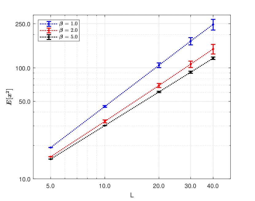
(b) Dimension 3

Figure 2: The power law dependence of the average squared length for H=0.5

This power law is quite evident in the figure, for three different values of the constant $\beta$ ($1.0,2.0$,$5.0$ and $H=0.5$). Notice that small values of $\beta$ correspond to situations of large phase space volume exclusion, while large values correspond to little or no exclusion. When the integrals in (22) and (23) are computed, as the value of $\beta$ decreases an increase in the error is expected, due to the increase in the weight of the exclusion. The same occurs when the length $L$ increases, due to the significant increase in the space over which the integration takes place.

Of most physical relevance is the asymptotic slope $\nu$ of

$$\sqrt{\mathbb{E}\left[x^{2}\left(L\right)\right]}\sim L^{\nu}$$ (25)

Fig.3 shows results for dimensions $n=2$ and $n=3$. Error bars in the figure account for statistical errors in the computation of the integrals. The important facts to retain are both the growth of the $\nu$ values with $H$ and their dependency on the range of the potential. The Flory [13] points ($\nu=0.75$ for $n=2$ and $\nu=0.6$ at $H=0.5$) are marked with ”$\bigcirc$” on the plots. They correspond to the situation where the average range of the potential is close to the size of a monomer (a discrete evolution step in our stochastic representation).

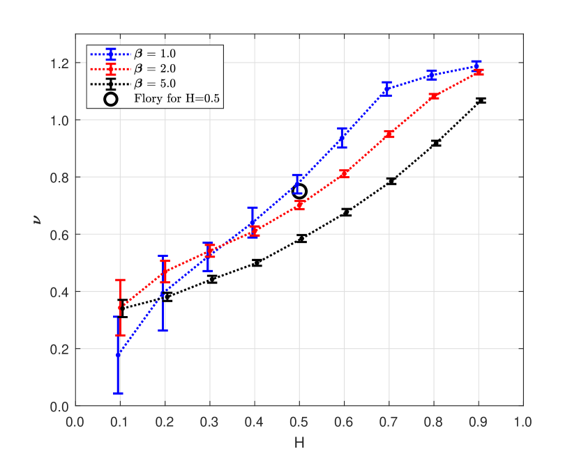
(a) Dimension 2

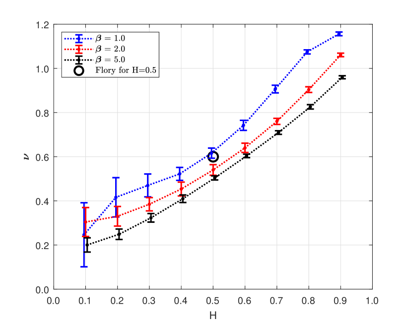
(b) Dimension 3

Figure 3: The scaling index

Because all integrals in (22-23) are Gaussian a closed form expression for $\mathbb{E}\left[x^{2}\left(L\right)\right]_{G}$ may in this case be obtained. First one expands the $\prod_{\alpha^{\prime}>\alpha\geq 1}^{L}$ product to obtain

$$\mathbb{E}\left[x^{2}\left(L\right)\right]_{G} = \frac{1}{Z}\int\left(\prod_{\alpha=1}^{L}d^{n}y_{\alpha}e^{-\frac{1}{2}\sum_{\alpha}\left|\overrightarrow{y}_{\alpha}\right|^{2}}\right)\left|\left\langle y|M_{L}^{(H)}\right\rangle\right|^{2}$$ (26)

$$\times\left(1+\sum_{p=1}^{M}\left(-1\right)^{p}\sum_{\begin{subarray}{c}\mathnormal{distinct}\text{ sets}\\ \text{of }p\text{ }\left(\alpha,\alpha\prime\right)\text{ pairs}\end{subarray}}e^{-\beta^{2}\sum_{p\text{ }\left(\alpha,\alpha\prime\right)\text{ pairs}}y\cdot A_{\alpha,\alpha^{\prime}}y}\right)$$

$$Z=\int\left(\prod_{\alpha=1}^{L}d^{n}y_{\alpha}e^{-\frac{1}{2}\sum_{\alpha}\left|\overrightarrow{y}_{\alpha}\right|^{2}}\right)\left(1+\sum_{p=1}^{M}\left(-1\right)^{p}\sum_{\begin{subarray}{c}\mathnormal{distinct}\text{ sets}\\ \text{of }p\text{ }\left(\alpha,\alpha\prime\right)\text{ pairs}\end{subarray}}e^{-\beta^{2}n\sum_{p\text{ }\left(\alpha,\alpha\prime\right)\text{ pairs}}y\cdot A_{\alpha,\alpha^{\prime}}y}\right)$$ (27)

where $M=\frac{L\left(L-1\right)}{2}$ and the matrices $A_{\alpha,\alpha^{\prime}}$ are a set of $M$ matrices that connect the space variables $y$ corresponding to the steps $\alpha$ and $\alpha^{\prime}$. As $nL\times nL$ matrices their elements are

$$\left(A_{\alpha,\alpha^{\prime}}\right)_{i\beta,j\beta^{\prime}}=\delta_{ij}\left(M_{\alpha}^{(H)}\left(\beta\right)-M_{\alpha^{\prime}}^{(H)}\left(\beta\right)\right)\left(M_{\alpha}^{(H)}\left(\beta^{\prime}\right)-M_{\alpha^{\prime}}^{(H)}\left(\beta^{\prime}\right)\right)$$ (28)

In (26) and (27) the integrals are Gaussian, leading to

$$\mathbb{E}\left[x^{2}\left(L\right)\right]_{G} = \frac{1}{Z}\frac{d}{d\gamma}\left(\det\left(\boldsymbol{1}-2B\gamma\right)^{-\frac{1}{2}}\right.$$ (29)

$$\left.\left.+\sum_{p=1}^{M}\left(-1\right)^{p}\sum_{\begin{subarray}{c}\mathnormal{distinct}\text{ sets}\\ \text{of }p\text{ }\left(\alpha,\alpha\prime\right)\text{ pairs}\end{subarray}}\det\left(\boldsymbol{1-}2B\gamma+2\beta^{2}n\sum_{p\text{ }\left(\alpha,\alpha\prime\right)\text{ pairs}}A_{\alpha,\alpha^{\prime}}\right)^{-\frac{1}{2}}\right)\right|_{\gamma=0}$$

and

$$Z=1+\sum_{p=1}^{M}\left(-1\right)^{p}\sum_{\begin{subarray}{c}\mathnormal{distinct}\text{ sets}\\ \text{of }p\text{ }\left(\alpha,\alpha\prime\right)\text{ pairs}\end{subarray}}\det\left(\boldsymbol{1}+2\beta^{2}\sum_{p\text{ }\left(\alpha,\alpha\prime\right)\text{ pairs}}A_{\alpha,\alpha^{\prime}}\right)^{-\frac{1}{2}}$$ (30)

$B$ is the matrix

$$\left(B\right)_{i\beta,j\beta^{\prime}}=\delta_{ij}M_{L}^{(H)}\left(\beta\right)M_{L}^{(H)}\left(\beta^{\prime}\right)$$

These closed form expressions are combinatorially complex, but may be used to check the results obtained directly from the integrals in (22) (23), at least for small $L$ values.

4.2 The step factor

Results for the step Gibbs factor are also relevant in particular because, as discussed before, this factor is essentially identical to the Edwards factor. It is also what is used in most Monte Carlo calculations

$$e^{-\phi_{step}\left(z\right)}=\theta\left(\left|z\right|^{2}-\varepsilon^{2}\right)$$ (31)

$\theta$ being the Heaviside function. Using (14) and (15) one writes

$$\mathbb{E}\left[x^{2}\left(L\right)\right]_{S}=\frac{1}{Z}\int\left(\prod_{\alpha=1}^{L}d^{n}y_{\alpha}e^{-\frac{1}{2}\sum_{\alpha}\left|\overrightarrow{y}_{\alpha}\right|^{2}}\right)\left|\left\langle\overrightarrow{y}|M_{L}^{(H)}\right\rangle\right|^{2}\prod_{\alpha^{\prime}>\alpha\geq 1}^{L}\theta\left(\left|\left\langle y|M_{\alpha}^{(H)}\right\rangle-\left\langle y|M_{\alpha^{\prime}}^{(H)}\right\rangle\right|^{2}-\varepsilon^{2}\right)$$ (32)

$$\mathbb{Z}=\int\left(\prod_{\alpha=1}^{L}d^{n}y_{\alpha}e^{-\frac{1}{2}\sum_{\alpha}\left|\overrightarrow{y}_{\alpha}\right|^{2}}\right)\prod_{\alpha^{\prime}>\alpha\geq 1}^{L}\theta\left(\left|\left\langle y|M_{\alpha}^{(H)}\right\rangle-\left\langle y|M_{\alpha^{\prime}}^{(H)}\right\rangle\right|^{2}-\varepsilon^{2}\right)$$

$\theta$ being the Heaviside function.

Here one obtains truncated Gaussian integrals: Given the correspondence $\beta\sim\frac{1}{\varepsilon}$, discussed before, we expect results similar to those of the Gaussian kernel, in particular also a dependency on the size of the cut-off $\varepsilon$. For example for $H=0.5$ we obtain for the $\nu$ exponent

$\begin{array}[]{lrr}&n=2&n=3\\ \varepsilon=0.1&0.54&\\ \varepsilon=0.33&0.64&\\ \varepsilon=0.4&0.69&0.52\\ \varepsilon=0.7&&0.55\\ \varepsilon=0.85&&0.58\end{array}$

Monte Carlo simulations with Brownian or fractional processes and a condition of minimal separation $\varepsilon$ for the polymer evolution, is equivalent to the step factor (31). Therefore the calculation of the integrals in (32) may be used as an alternative to Monte Carlo simulations.

Acknowledgments

Partially supported by Fundação para a Ciência e a Tecnologia (FCT), project UIDB/04561/2020: https://doi.org/10.54499/UIDB/04561/2020

References

- [1] R. Brown, Robert; A brief account of microscopical observations made in the months of June, July and August, 1827, on the particles contained in the pollen of plants; and on the general existence of active molecules in organic and inorganic bodies, Philosophical Magazine 4 (1828) 161-173.
- [2] L. Bachelier; Théorie de la spéculation, Annales Scientifiques de l’École Normale Supérieure 3 (1900) 21-86.
- [3] A. Einstein; Über die von der molekularkinetischen Theorie der Wärme geforderte Bewegung von in ruhenden Flüssigkeiten suspendierten Teilchen, Annalen der Physik 322 (1905) 549-560.
- [4] T. Hida, H.-H. Kuo, J. Potthoff and L. Streit; White Noise: An Infinite Dimensional Calculus, Springer Dordrecht, 2010.
- [5] Y. LeJan and A. S. Sznitman; Stochastic cascades and 3-dimensional Navier–Stokes equations, Prob. Theory and Relat. Fields 109 (1997) 343-366.
- [6] E. C. Waymire; Probability & incompressible Navier-Stokes equations: An overview of some recent developments, Prob. Surveys 2 (2005) 1-32.
- [7] E. Floriani and R. Vilela Mendes; A stochastic approach to the solution of magnetohydrodynamic equations, Journal of Computational Physics 242 (2013) 777–789.
- [8] F. Cipriano, H. Ouerdiane and R. Vilela Mendes; Stochastic solution of a KPP-type nonlinear fractional differential equation, Fractional Calculus and Applied Analysis 12 (2009) 47–56.
- [9] R. Vilela Mendes; Stochastic solutions and singular partial differential equations, Communications in Nonlinear Science and Numerical Simulation 125 (2023) 107406.
- [10] S. F. Edwards; The statistical mechanics of polymers with excluded volume, Proc. Phys. Soc. 85 (1965) 613-624.
- [11] P. J. Flory; Thermodynamics of High Polymer Solutions, Journal of Chemical Physics 9 (1941) 660-661.
- [12] M. L. Huggins; Solutions of Long Chain Compounds, Journal of Chemical Physics 9 (1941) 440.
- [13] P. Flory; Selected Works of Paul J. Flory, Stanford Univ Press. 1985.
- [14] F. Biagini, B. Øksendal, A. Sulem and N. Wallner; An Introduction to White-Noise Theory and Malliavin Calculus for Fractional Brownian Motion, Proc. R. Soc. Lond. A 460 (2004) 347-372.
- [15] Y. Mishura; Stochastic Calculus for Fractional Brownian Motion and Related Processes, Springer LNM 1929, Berlin 2008.
- [16] I. Norros, E. Valkeila and J. Virtamo; An elementary approach to a Girsanov formula ans other analytical results on fractional Brownian motion, Bernoulli 5 (1999) 571-587.
- [17] Y. Mishura and K. Ralchenko; Discrete-Time Approximations and Limit Theorems; De Gruyter, Berlin 2022.
- [18] M. Grothaus, M. J. Oliveira, J. L. Silva and L. Streit; Self-avoiding fractional Brownian motion - The Edwards model, J. Stat. Phys. 145 (2011) 1513-1523.
- [19] S. R. S. Varadhan; Appendix to ”Euclidean quantum field theory” by K. Symanzik, in R. Jost (ed.) Local Quantum Theory, Academic Press, p. 285, New York 1970.
- [20] M. Yor; Renormalisation et convergence en loi pour les temps locaux d’intersection du movement Brownien dans ; Lectures Notes in Math. 1123 (1985) 350-365.
- [21] J. Y. Calais and M. Yor; Renormalisation et convergence en loi pour certains intégrales multiples associés au mouvement Brownien dans , Lecture Notes in Mat. 1247 (1987) 375-403.
- [22] Y. Hu and D. Nualart; Renormalized self-intersection local time for fractional Brownian motion, Ann. Proba. 33 (2005) 948-983.
- [23] Y. Hu and D. Nualart; Regularity of renormalized self-intersection local time for fractional Brownian motion, Commun. Inf. Syst. 7 (2007) 21-30.
- [24] M. J. Oliveira, J. L. Silva and L. Streit; Intersection local times of independent fractional Brownian motions as generalized white noise functionals, Acta Appl.Math. 113 (2011) 17-39.
- [25] B. Alberts, D. Bray, J. Lewis, M. Raff, K. Roberts and J. D. Watson; Molecular Biology of the Cell, Garland, New York 1994.