Estimating Peer Direct and Indirect Effects in Observational Network Data

Abstract

Estimating causal effects is crucial for decision-makers in many applications, but it is particularly challenging with observational network data due to peer interactions. Many algorithms have been proposed to estimate causal effects involving network data, particularly peer effects, but they often overlook the variety of peer effects. To address this issue, we propose a general setting which considers both peer direct effects and peer indirect effects, and the effect of an individual’s own treatment, and provide identification conditions of these causal effects and proofs. To estimate these causal effects, we utilize attention mechanisms to distinguish the influences of different neighbors and explore high-order neighbor effects through multi-layer graph neural networks (GNNs). Additionally, to control the dependency between node features and representations, we incorporate the Hilbert-Schmidt Independence Criterion (HSIC) into the GNN, fully utilizing the structural information of the graph, to enhance the robustness and accuracy of the model. Extensive experiments on two semi-synthetic datasets confirm the effectiveness of our approach. Our theoretical findings have the potential to improve intervention strategies in networked systems, with applications in areas such as social networks and epidemiology.

Introduction

Causal effect estimation is an important area of study, with the focus on determining cause-and-effect relationships between variables (Imbens and Rubin 2010; Pearl 2009). It is challenging to achieve accurate causal effect estimation using observational data due to the presence of confounders that affect both the treatment and the outcome. When the data is collected from sources such as social networks, communication networks, or biological networks, causal effect estimation becomes even more challenging since the data is inherently networked, meaning that units (e.g., individuals, nodes) are interconnected, and their outcomes potentially being influenced by both the treatments and outcomes of their neighbors (Sinclair, McConnell, and Green 2012). This implies that traditional causal inference methods are not applicable any more since they may not adequately account for peer effects or network dependencies (Yao et al. 2021). Therefore, estimating causal effects on network data necessitates specialized techniques that can handle these interdependencies, ensuring that the estimated effects are not biased by the network structure itself.

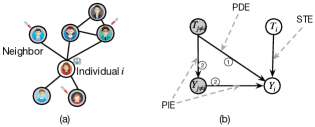
Figure 1: (a) A graph to showing the relationship between individual $i$ and their neighbors in network data. (b) A causal graph illustrating peer direct effects (PDE), peer indirect effects (PIE), and self-treatment effects (STE). In the diagram, $T$ and $Y$ indicate the intervention (e.g., vaccination status and infection condition), the subscript $i$ indicates an individual and ${j\neq i}$ indicates their neighbours.

Effects in network data can be classified into peer effects (PE, an individual’s treatment affects another’s outcome) and self-treatment effects (STE, an individual’s treatment affects their own outcome). As illustrated in Fig. 1(a), in the context of an infectious disease, an individual’s infection status depends on both their own and their neighbors’ vaccination statuses. Peer effects can be direct, where the vaccination of an individual’s neighbour reduces the risk of the individual’s infection (peer direct effect, PDE, as indicated by the edge marked with \scriptsize{1}⃝ in Fig. 1(b)), or indirect, where the vaccination of an individual’s neighbour affects the neighbor’s own infection status, which in turn (indirectly) affects the individual’s infection status (peer indirect effect, PIE, as indicated by the path marked with \scriptsize{2}⃝ in Fig. 1(b)). Understanding these mechanisms is crucial for optimizing vaccination strategies. Peer direct effect denotes the effectiveness of a vaccine on an individual by vaccinating their neighbours regardless of their neighbours’ infectious conditions. Peer indirect effect indicates the effectiveness of a vaccine on an individual by improving their neighbours infectious conditions through vaccination.

Method	Type of Relationship	Causal Effects Considered
VanderWeele (VanderWeele, Tchetgen, and Halloran 2012)	Unidirectional, one to one	PDE, PIE
Shpitser (Shpitser, Tchetgen, and Andrews 2017)	Bidirectional, one to one	PDE, PIE
NetEst (Jiang and Sun 2022), Cai (Cai et al. 2023), TNet (Chen et al. 2024)	Many to one (at group level)	PE, STE
gDIS (ours)	Many to one (at group level)	PDE, PIE, STE

Table 1: Comparison of problem settings across different methods. Methods are identified by the authors’ names when the method name is not specified in the original text.

Causal mediation analysis (MacKinnon, Fairchild, and Fritz 2007) is usually used to distinguish between direct and indirect effects in independent and identically distributed (IID) data. VanderWeele et al. (VanderWeele, Tchetgen, and Halloran 2012) combined causal mediation analysis with statistical models to explore how vaccinating a one-year-old child might affect the child’s mother, especially within a two-person household. Shpitser et al. (Shpitser, Tchetgen, and Andrews 2017) further advanced this approach by developing a symmetric treatment decomposition method based on chain graphs to address peer effects. This method enables the analysis of complex scenarios involving mutual influence, such as the interaction between a child and their mother. It allows the overall peer effect to be decomposed into specific components, facilitating the analysis of how interference effects are transmitted between individuals and helping to distinguish between direct and indirect effects.

Jiang et al. (Jiang and Sun 2022) formalized the estimation of network causal effects as a multi-task learning problem and introduced a framework called Networked Causal Effects Estimation (NetEst). This method utilizes GNNs (Hu et al. 2020) to capture feature representations of both individual and their first-order neighbors. Cai et al. (Cai et al. 2023) derived generalization bounds for causal effect estimates from network data and proposed a weighted regression strategy based on joint propensity scores (Lee, Lessler, and Stuart 2010) combined with representation learning. Chen et al. (Chen et al. 2024) integrated the targeted learning (Van der Laan, Rose et al. 2011) into neural network training, developing a causal effect estimator.

As shown in Table 1, although VanderWeele et al. (VanderWeele, Tchetgen, and Halloran 2012) and Shpitser et al. (Shpitser, Tchetgen, and Andrews 2017) considered both peer direct effects and indirect effects, their work primarily focused on scenarios with a propagation unit of two people only, which limits their practical applicability. Additionally, they did not account for STE, which are significant in networks and crucial for policy-making in interventions. While the recent work by Jiang et al. (Jiang and Sun 2022), Cai et al. (Cai et al. 2023), and Chen et al. (Chen et al. 2024) considered group-level peer effects, they did not differentiate between the various types of peer effects. In many cases, particularly in infectious diseases, it is not enough to simply know that overall peer effects. It is important to distinguish between PDE and PIE, as each has different implications.

To address these limitations, we consider a more general setting for observational network data, where we estimate PDE and PIE at group level, as well as STE within networks. We apply the principles of mediation analysis (Pearl 2014) and the backdoor criterion (Pearl 2009) to analyze these effects, and provide their identification conditions and the proofs. Based on the theoretical analysis, we develop gDIS for group-level PDE and PIE, and STE estimation with network data. To effectively capture the complexity of network effects, gDIS employs a multi-layer GNN to focus on high-order neighbor interference and leverages the potential of attention mechanisms (Niu, Zhong, and Yu 2021) to account for the varying influence weights of different neighbors on each individual. Furthermore, to better control the dependency relationships between node features, we integrate the Hilbert-Schmidt Independence Criterion (HSIC) (Ahmad, Mazzara, and Distefano 2021) into the GNN, fully leveraging the structural information of computational graphs.

Our main innovations are summarized as follows:

• We propose to decompose peer effects into direct and indirect components at the group level in observational network data, and provide both the theoretical analyses and the corresponding proofs for the identifiability of these effects .

• We develop a novel method gDIS for estimating the two different types of peer effects at group level and the self-treatment effect, using network data.

• We validated the effectiveness and robustness of the gDIS on semi-synthetic datasets, showing that it maintains great performance even in complex network data.

Preliminary

This section provides the notations and problem setting used throughout the paper.

Notations and Problem Setting

Throughout the paper, uppercase letters (e.g., $T_{i}$, $W_{t_{i}}$) denote variables, while lowercase letters (e.g., $t_{i}$, $w_{t_{i}}$) represent their values. Bold uppercase letters (e.g., $\mathbf{W}_{x}$, $\mathbf{X}$, $\mathbf{W}_{y}$, $\mathbf{W}_{x_{i}}$) indicate sets of variables, vectors or matrices, and bold lowercase letters (e.g., $\mathbf{w}_{x}$, $\mathbf{x}$, $\mathbf{w}_{y}$, $\mathbf{w}_{x_{i}}$) represent their corresponding values.

A network can be represented as a pair $(\mathbf{V},\mathbf{E})$, where $\mathbf{V}=\{V_{1},\ldots,V_{m}\}$ is the set of nodes, and $\mathbf{E}\subseteq\mathbf{V}\times\mathbf{V}$ is the set of edges between the nodes. A node $V_{i}\in\mathbf{V}$ has a set of features $\mathbf{X}_{i}=\{X_{i1},\ldots,X_{ik}\}$, a treatment $T_{i}$, and an outcome $Y_{i}$ associated with it. We assume $T_{i}\in\{0,1\}$ is a binary treatment, representing, e.g., whether node $V_{i}$ receives a vaccination or not, and $Y_{i}$ is a continuous variable, indicating, e.g., the level of immunity of $V_{i}$. For simplicity of presentation, we will use the index of a node, e.g., $i$, to represent the corresponding node $V_{i}$ when there is no ambiguity in the rest of the paper.

Considering an individual or node $i$, its outcome $Y_{i}$ is affected by several factors: its own features $\mathbf{X}_{i}$, its treatment $T_{i}$, the features of its neighbors $\{\mathbf{X}_{j}\}_{j\in\mathcal{N}_{i}}$, the treatments administered to those neighbors $\{T_{j}\}_{j\in\mathcal{N}_{i}}$, and the outcomes observed in those neighbors $\{Y_{j}\}_{j\in\mathcal{N}_{i}}$. Here, $\mathcal{N}_{i}$ represents the set of neighbors of unit $i$, as illustrated in Fig. 2(a).

We use Kullback-Leibler (KL) divergence (Belov and Armstrong 2011) to compute the difference between the probability distributions $P_{i}$ and $P_{j}$ of node $i$ and its neighboring node $j$, as given by Eq 1 below:

$$D_{\text{KL}}(P_{i}\parallel P_{j})=\sum_{k}P_{i}(k)\log(\frac{P_{i}(k)}{P_{j}(k)})$$ (1)

where $k$ is the dimension of the feature vector of a node.

Based on the KL divergence, we calculate the influence weight of neighbor $j$ on individual $i$, $w_{ij}$ as follows:

$$w_{ij}=\frac{1}{1+D_{\text{KL}}(P_{i}\parallel P_{j})}$$ (2)

The higher the weight $w_{ij}$, the greater the influence of neighbor $j$ on individual $i$.

Neighbor treatment exposure $W_{t_{i}}$, neighbor contagion exposure $W_{y_{i}}$, and neighbor feature $\mathbf{W}_{x_{i}}$ are calculated as: $W_{t_{i}}=\sum_{j\in\mathcal{N}_{i}}w_{ij}T_{j}$, $W_{y_{i}}=\sum_{j\in\mathcal{N}_{i}}w_{ij}Y_{j}$, $\mathbf{W}_{x_{i}}=\sum_{j\in\mathcal{N}_{i}}w_{ij}\mathbf{X}_{j}$, respectively.

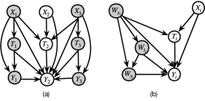
Figure 2: (a) An illustration of the causal relationships considered in our work, for node 2, which has node 1 and 3 as neighbours in the network. The features, treatment, and outcome of node $i$ are represented by $X_{i}$, $T_{i}$, and $Y_{i}$, respectively. (b) The summary causal graph where $W_{x_{i}}$, $W_{t_{i}}$, and $W_{y_{i}}$ represent the aggregated features, treatments, and outcomes of node $i$’s neighbors.

Our problem definition is provided as follows:

Problem Definition. Given the observational networked data of a network $(\textbf{V},\textbf{E})$, including the data of the features, treatments and outcomes associated with the nodes of the network, our goal is for each node or individual $i$ to distinguish and obtain unbiased estimation of the peer direct effects (PDE) (i.e., the causal effect of $W_{t_{i}}$ on $Y_{i}$ via $W_{t_{i}}\rightarrow Y_{i}$), peer indirect effects (PIE) (i.e., the causal effect of $W_{t_{i}}$ on $Y_{i}$ via $W_{t_{i}}\rightarrow W_{y_{i}}\rightarrow Y_{i}$), and self-treatment effects (STE) (i.e., the causal effect of $T_{i}$ on $Y_{i}$ via $T_{i}\rightarrow Y_{i}$) as shown in Fig. 2.

The formal definitions of group level PDE and PIE, and STE are based on the potential outcome framework (Imbens and Rubin 2010). In the following, we first present the basic concepts of the framework, then give the definitions of PDE, PIE and STE.

For each unit $i$ under two treatment conditions $T_{i}$ (where $T_{i}=0$ represents no treated unit and $T_{i}=1$ represents treated unit), we define two potential outcomes: $Y_{i}(1)$, the outcome if the unit receives treatment, and $Y_{i}(0)$, the outcome if untreated.

The individual treatment effect (ITE) is defined as the difference between these potential outcomes:

$$\mathrm{ITE}_{i}=Y_{i}(1)-Y_{i}(0)$$ (3)

The average treatment effect (ATE) across the population is defined as the expected value of the ITE for all units:

$$\mathrm{ATE}=\mathbb{E}[Y_{i}(1)-Y_{i}(0)]$$ (4)

Under the potential outcome framework and following the definitions of PDE and PIE in (VanderWeele, Tchetgen, and Halloran 2012), in our problem setting, we have:

$$\mathrm{PDE}=\mathbb{E}\left[Y_{i}(w_{t_{i}}^{\prime},{W}_{y}(w_{t_{i}}^{\prime}))-Y(w_{t_{i}},{W}_{y}(w_{t_{i}}^{\prime})\right]$$ (5)

$$\mathrm{PIE}=\mathbb{E}\left[Y_{i}(w_{t_{i}},{W}_{y}(w_{t_{i}}^{\prime})-Y_{i}(w_{t_{i}},{W}_{y}(w_{t_{i}}))\right]$$ (6)

The PDE defined in Eq. 5 indicates the average of the difference between the potential outcomes of an individual when the aggregated treatment of its neighbours, i.e., its neighbor treatment exposure $W_{t_{i}}$, is changed from one level ($w_{t_{i}}$) to another ($w_{t_{i}}^{\prime}$), while the aggregated neighbor potential outcome, i.e., its neighbor contagion exposure $W_{y_{i}}$, remains at the level as it would have been if the neighbours’ aggregated treatment had been $w_{t_{i}}^{\prime}$, denoted as $w_{y}(w_{t_{i}}^{\prime})$. In the vaccination example, PDE indicates the average effect of changing the vaccination status of an individual’s neighbors on the infectious status of the individual, assuming the neighbors’ infectious status is kept at the level as after their vaccination status is changed.

The PIE defined in Eq. 6 indicates the average of the difference between the potential outcomes of an individual when the aggregated treatment of its neighbours, i.e., its neighbor treatment exposure $W_{t_{i}}$, remains unchanged at ($w_{t_{i}}$), while the aggregated neighbor potential outcome, i.e., its neighbor contagion exposure $W_{y_{i}}$, is changed from what it would have been if the neighbours’ aggregated treatment had been $w_{t_{i}}^{\prime}$, denoted as $w_{y}(w_{t_{i}}^{\prime})$, to what it would have been if the neighbours’ aggregated treatment had been $w_{t_{i}}$, i.e., $w_{y}(w_{t_{i}})$. In the vaccination example, PIE indicates that assuming the vaccination status of the neighbors of an individual remains unchanged, how the change of the infectious status of an individual’s neighbors as a result of changing their vaccination status would affect the infectious status of the individual.

The definition of STE in our problem setting is similar to the definition of ATE, i.e., $\mathrm{STE}=\mathbb{E}\left[Y_{i}(1)-Y_{i}(0)\right]$. In the vaccination example, STE indicates the average difference of potential outcomes of an individual if the individual had been vaccinated versus if they had not been vaccinated.

Estimating these effects deepens our understanding of interactions within complex networks and provides critical insights for informed policy decisions.

Assumptions

In observational data, we only have the observed outcome, i.e., the factual outcome, but estimating causal effects requires the potential outcomes, i.e., both the factual and counterfactual outcomes. Therefore, the following assumptions are needed for estimating causal effects from observational network data (Jiang and Sun 2022).

In the following assumptions, $Z_{i}=(W_{t_{i}},W_{y_{i}})$, where $W_{t_{i}}$ and $W_{y_{i}}$ represent the aggregated treatment and contagion exposures of node $i$’s neighbors, respectively. We define $z_{i}$ as the corresponding value of $Z_{i}$.

Assumption 1 (Network Unconfoundedness): The potential outcome is independent of both individual treatment and neighborhood exposure, given the individual and neighbor features. i.e., $Y_{i}(t_{i},z_{i})\perp\!\!\!\perp t_{i},z_{i}\mid\mathbf{X}_{i},\mathbf{W}_{x_{i}}$.

Assumption 2 (Network Interference): If the potential outcome $Y_{i}(t_{i},z_{i})$ for individual $i$ depends on both $i$’s treatment $T_{i}$ and $Z_{i}$, network interference exists.

Assumption 3 (Network Consistency): The potential outcome equals the observed outcome when a unit is exposed to the same treatment and neighborhood exposure. i.e., $Y_{i}=Y_{i}(t_{i},z_{i})$ if unit $i$ is subjected to $t_{i}$ and $z_{i}$.

Assumption 4 (Network Overlap): Every treatment and neighborhood exposure pair $(T_{i},Z_{i})$ must have a positive probability of occurring. i.e., $0<p(t_{i},z_{i}\mid\mathbf{X}_{i},\mathbf{W}_{x_{i}})<1$.

The Proposed gDIS Method

Identifiability of PDE, PIE and STE

Establishing the identifiability of a causal effects is the prerequisite for estimating the causal effects from data. To study the identifiability of the causal effects (PDE, PIE and STE) with network data, we propose a novel causal graph, as shown in Fig. 2(b), to illustrate these causal effects. In this section, we provide the assumptions and conditions for identifying these causal effects from network data, along with the theoretical analysis and corresponding proofs.

To present our main theoretical results (Theorems 1 and 2 below), we make the following assumptions, which are commonly found in the causal inference literature and adapted to our problem setting, with causal relationships between variables illustrated in Fig. 2(b). For simplicity, we omit the subscript $i$ from the names of the variables shown in Fig. 2(b) in the following discussion.

Assumption 5

(Sequential Ignorability (Imai, Keele, and Yamamoto 2010)) There exists a set of observed covariates $\mathbf{W}$ such that:

1_G-1. $\mathbf{W}$ and $\mathbf{W}_{t}$ block all backdoor paths from $\mathbf{W}_{y}$ to $\mathbf{Y}$ that do not pass through $\mathbf{W}_{t}$;

1_G-2. The set $\mathbf{W}$ blocks all backdoor paths from $\mathbf{W}_{t}$ to $\mathbf{W}_{y}$ or $\mathbf{Y}$, and no element in $\mathbf{W}$ is a descendant of $\mathbf{W}_{t}$.

A set $\mathbf{W}$ that satisfies both conditions in Assumption 5 serves as an adjustment set for obtaining unbiased estimates of PDE and PIE from network data. We present our first theoretical finding below.

Theorem 1.

In the causal DAG represented in Fig 2(b), the set of neighbor features $\mathbf{W}_{x}$ satisfies both conditions 1_G-1 and 1_G-2 of Assumption 5.

Proof: First, we prove that $\{\mathbf{W}_{x}\}$ satisfies condition 1_G-1 of Assumption 5. In the causal DAG shown in Fig. 2(b), all $\mathbf{W}_{t}$-avoiding backdoor paths from $\mathbf{W}_{y}$ to $\mathbf{Y}$ ($\mathbf{W}_{y}\leftarrow\mathbf{W}_{x}\rightarrow\mathbf{Y}$, $\mathbf{W}_{y}\leftarrow\mathbf{W}_{x}\rightarrow\mathbf{T}\leftarrow\mathbf{X}\rightarrow\mathbf{Y}$, and $\mathbf{W}_{y}\leftarrow\mathbf{W}_{x}\rightarrow\mathbf{T}\rightarrow\mathbf{Y}$) are blocked by the set $\{\mathbf{W}_{x},\mathbf{W}_{t}\}$, thus $\{\mathbf{W}_{x}\}$ satisfies 1_G-1. Next, we prove that $\{\mathbf{W}_{x}\}$ satisfies condition 1_G-2. The set $\{\mathbf{W}_{x}\}$ blocks all backdoor paths from $\mathbf{W}_{t}$ to $\mathbf{W}_{y}$ ($\mathbf{W}_{t}\leftarrow\mathbf{W}_{x}\rightarrow\mathbf{W}_{y}$, $\mathbf{W}_{t}\leftarrow\mathbf{W}_{x}\rightarrow\mathbf{Y}\leftarrow\mathbf{W}_{y}$, $\mathbf{W}_{t}\leftarrow\mathbf{W}_{x}\rightarrow\mathbf{T}\leftarrow\mathbf{Y}\leftarrow\mathbf{W}_{y}$, and $\mathbf{W}_{t}\leftarrow\mathbf{W}_{x}\rightarrow\mathbf{T}\leftarrow\mathbf{X}\rightarrow\mathbf{Y}\leftarrow\mathbf{W}_{y}$) and from $\mathbf{W}_{t}$ to $\mathbf{Y}$ ($\mathbf{W}_{t}\leftarrow\mathbf{W}_{x}\rightarrow\mathbf{Y}$, $\mathbf{W}_{t}\leftarrow\mathbf{W}_{x}\rightarrow\mathbf{W}_{y}\rightarrow\mathbf{Y}$, $\mathbf{W}_{t}\leftarrow\mathbf{W}_{x}\rightarrow\mathbf{T}\rightarrow\mathbf{Y}$, and $\mathbf{W}_{t}\leftarrow\mathbf{W}_{x}\rightarrow\mathbf{T}\leftarrow\mathbf{X}\rightarrow\mathbf{Y}$). $\mathbf{W}_{x}$ is not a descendant of $\mathbf{W}_{t}$ in Fig. 2(b) and satisfies 1_G-2. Therefore, $\mathbf{W}_{x}$ satisfies Assumption 5 and is an adjustment set for unbiasedly estimating the PDE and PIE.

Based on Theorem 1, the counterfactual expressions for PDE (Eq. 5), PIE (Eq. 6), and STE can be simplified into the do-expressions. This leads to our second theoretical finding presented below.

$$\mathrm{PDE}=\mathbb{E}\left[\mathbf{Y}\mid\mathrm{do}(\mathbf{W}_{t}=\mathbf{w}_{t}^{\prime},\mathbf{W}_{y}=\mathbf{w}_{y}^{\prime}),\mathbf{W}_{x}=\mathbf{w}_{x})\right]$$

$$\quad-\mathbb{E}\left[\mathbf{Y}\mid\mathrm{do}(\mathbf{W}_{t}=\mathbf{w}_{t},\mathbf{W}_{y}=\mathbf{w}_{y}^{\prime}),\mathbf{W}_{x}=\mathbf{w}_{x})\right]$$

$$\quad\times P(\mathbf{W}_{y}=\mathbf{w}_{y}^{\prime}\mid\mathrm{do}(\mathbf{W}_{t}=\mathbf{w}_{t}^{\prime}),\mathbf{W}_{x}=\mathbf{w}_{x})$$

$$\quad\times P(\mathbf{W}_{x}=\mathbf{w}_{x})$$ (7)

$$\mathrm{PIE}=\mathbb{E}\left(\mathbf{Y}\mid\mathrm{do}(\mathbf{W}_{t}=\mathbf{w}_{t},\mathbf{W}_{y}=\mathbf{w}_{y}),\mathbf{W}_{x}=\mathbf{w}_{x}\right)$$

$$\quad\times\left[P(\mathbf{W}_{y}=\mathbf{w}_{y}\mid\mathrm{do}(\mathbf{W}_{t}=\mathbf{w}_{t}^{\prime}),\mathbf{W}_{x}=\mathbf{w}_{x})\right.$$

$$\quad\left.-P(\mathbf{W}_{y}=\mathbf{w}_{y}\mid\mathrm{do}(\mathbf{W}_{t}=\mathbf{w}_{t}),\mathbf{W}_{x}=\mathbf{w}_{x})\right]$$ (8)

$$\mathrm{STE}=E(\mathbf{Y}\mid\mathrm{do}(\mathbf{T}=\mathbf{t}^{\prime}))-E(Y\mid\mathrm{do}(\mathbf{T}=\mathbf{t}))$$ (9)

Based on Pearl’s back-door adjustment formula and rules of do-calculus (Pearl 2009), we have the theorem 1 to simplify do-expressions into probability expressions.

Theorem 2.

If we can derive $p(\mathbf{T},\mathbf{Y},\mathbf{X},\mathbf{W}_{x},\mathbf{W}_{y},\mathbf{W}_{t}$ from the causal DAG in Fig 2(b), then the PDF, PIE and STE can be identified from the data as follow:

$$\mathrm{PDE}=\left[E(\mathbf{Y}\mid\mathbf{W}_{t}=\mathbf{w}_{t}^{\prime},\mathbf{W}_{y}=\mathbf{w}_{y}^{\prime},\mathbf{W}_{x}=\mathbf{w}_{x})\right.$$

$$\quad\left.-E(\mathbf{Y}\mid\mathbf{W}_{t}=\mathbf{w}_{t},\mathbf{W}_{y}=\mathbf{w}_{y}^{\prime},\mathbf{W}_{x}=\mathbf{w}_{x})\right]$$

$$\quad\times P(\mathbf{W}_{y}=\mathbf{w}_{y}^{\prime}\mid\mathbf{W}_{t}=\mathbf{w}_{t}^{\prime},\mathbf{W}_{x}=\mathbf{w}_{x})$$

$$\quad\times P(\mathbf{W}_{x}=\mathbf{w}_{x})$$ (10)

$$\mathrm{PIE}=E(\mathbf{Y}\mid\mathbf{W}_{t}=\mathbf{w}_{t},\mathbf{W}_{y}=\mathbf{w}_{y},\mathbf{W}_{x}=\mathbf{w}_{x})$$

$$\quad\times\left[P(\mathbf{W}_{y}=\mathbf{w}_{y}\mid\mathbf{W}_{t}=\mathbf{w}_{t}^{\prime},\mathbf{W}_{x}=\mathbf{w}_{x})\right.$$

$$\quad\left.-P(\mathbf{W}_{y}=\mathbf{w}_{y}\mid\mathbf{W}_{t}=\mathbf{w}_{t},\mathbf{W}_{x}=\mathbf{w}_{x})\right]$$ (11)

$$\mathrm{STE}=P(\mathbf{X}=\mathbf{x})P(\mathbf{W}_{x}=\mathbf{w}_{x})$$

$$\quad\times\left[E(\mathbf{Y}\mid\mathbf{T}=\mathbf{t}^{\prime},\mathbf{X}=\mathbf{x},\mathbf{W}_{x}=\mathbf{w}_{x})\right.$$

$$\quad\left.-E(\mathbf{Y}\mid\mathbf{T}=\mathbf{t},\mathbf{X}=\mathbf{x},\mathbf{W}_{x}=\mathbf{w}_{x})\right]$$ (12)

Proof: We prove that Eq Theorem 1. to Eq 9 are identifiable, i.e., the do-operator can be converted to a do-free expression in Eq Theorem 2. to Eq Theorem 2., respectively. Our proposed causal DAG is shown in Fig 2(b). Based on rule 2 of do-calculus, we have $P(\mathbf{Y}\ =\mathbf{y}\ \mid\text{do}(\mathbf{W}_{t}=\mathbf{w}_{t}^{\prime},\mathbf{W}_{y}=\mathbf{w}_{y}^{\prime}),\mathbf{W}_{x}=\mathbf{w}_{x}))=P(\mathbf{Y}\ =\mathbf{y}\mid\text{do}(\mathbf{W}_{t}=\mathbf{w}_{t}^{\prime}),\mathbf{W}_{y}=\mathbf{w}_{y}^{\prime},\mathbf{W}_{x}=\mathbf{w}_{x}))$ since $(\mathbf{Y}\ \perp\!\!\!\perp\mathbf{W}_{y}\mid\mathbf{W}_{t},\mathbf{W}_{x})_{G_{\overline{\mathbf{W}_{t}}\underline{\mathbf{W}_{y}}}}$, where $\overline{\mathbf{W}_{t}}$ represents the removal of all arrows pointing to $\mathbf{W}_{t}$, and $\underline{\mathbf{W}_{y}}$ represents the removal of all arrows emanating from $\mathbf{W}_{y}$. $P(\mathbf{Y}\ =\mathbf{y}\mid\text{do}(\mathbf{W}_{t}=\mathbf{w}_{t}^{\prime}),\mathbf{W}_{y}=\mathbf{w}_{y}^{\prime},\mathbf{W}_{x}=\mathbf{w}_{x}))=P(\mathbf{Y}\ =\mathbf{y}\mid\mathbf{W}_{t}=\mathbf{w}_{t}^{\prime},\mathbf{W}_{y}=\mathbf{w}_{y}^{\prime},\mathbf{W}_{x}=\mathbf{w}_{x}))$ because $(\mathbf{Y}\ \perp\!\!\!\perp\mathbf{W}_{t}\mid\mathbf{W}_{y},W_{x})_{G_{\underline{\mathbf{W}_{t}}}}$, where $\underline{\mathbf{W}_{t}}$ represents the removal of all arrows emanating from $\mathbf{W}_{t}$. $P(\mathbf{W}_{y}=\mathbf{w}_{y}^{\prime}\mid\text{do}(\mathbf{W}_{t}=\mathbf{w}_{t}^{\prime}),\mathbf{W}_{x}=\mathbf{w}_{x}))=P(\mathbf{W}_{y}=\mathbf{w}_{y}^{\prime}\mid\mathbf{W}_{t}=\mathbf{w}_{t}^{\prime},\mathbf{W}_{x}=\mathbf{w}_{x}))$ because $(\mathbf{W}_{y}\perp\!\!\!\perp\mathbf{W}_{t}\mid\mathbf{W}_{x})_{G_{\underline{\mathbf{W}_{t}}}}$.

Based on the back-door adjustment formula, $P(\mathbf{Y}=\mathbf{y}\mid\text{do}(\mathbf{T}=\mathbf{t}^{\prime}))$ is identifiable because all backdoor paths from $\mathbf{T}$ to $\mathbf{Y}$ are blocked by adjusting for $\mathbf{X}$ and $\mathbf{W}_{x}$. Specifically, $\mathbf{T}\leftarrow\mathbf{X}\rightarrow\mathbf{Y}$ is blocked by $\mathbf{X}$, $\mathbf{T}\leftarrow\mathbf{W}_{x}\rightarrow\mathbf{W}_{t}\rightarrow\mathbf{Y}$ is blocked by $\mathbf{W}_{x}$, $\mathbf{T}\leftarrow\mathbf{W}_{x}\rightarrow\mathbf{W}_{t}\rightarrow\mathbf{W}_{y}\rightarrow\mathbf{Y}$ is blocked by $\mathbf{W}_{x}$, $\mathbf{T}\leftarrow\mathbf{W}_{x}\rightarrow\mathbf{W}_{y}\rightarrow\mathbf{Y}$ is blocked by $\mathbf{W}_{x}$, and $\mathbf{T}\leftarrow\mathbf{W}_{x}\rightarrow\mathbf{W}_{y}\leftarrow\mathbf{W}_{t}\rightarrow\mathbf{Y}$ is blocked by $\mathbf{W}_{x}$. Hence, $P(\mathbf{Y}=\mathbf{y}\mid\text{do}(\mathbf{T}=\mathbf{t}^{\prime}))=P(\mathbf{Y}=\mathbf{y}\mid\mathbf{T}=\mathbf{t}^{\prime})P(\mathbf{X}=\mathbf{x})P(\mathbf{W}_{x}=\mathbf{w}_{x})$. For details on the processes for calculating the PDE, PIE, and STE, please refer to the Appendix due to page limit.

Implementation

To accurately estimate PDE, PIE, and STE within networks, it is first necessary to establish Theorem 2, proving that these effects can be effectively identified, and then derive Eq Theorem 2. to Eq Theorem 2.. The implementation process involves three key steps: (1-1) Causal Mediation Analysis: This step decomposes network peer effects into direct and indirect effects using causal mediation analysis (Pearl 2014); (1-2) Back-Door Criterion Adjustment: This step effectively identifies the STE using the back-door criterion, as introduced in the preliminaries. (2) GNNs: Multi-layer GNNs with attention mechanisms are employed to capture the different influence of high-order neighbors. (3) HSIC Regularization: HSIC regularization (Ahmad, Mazzara, and Distefano 2021) is integrated to ensure independence between features and embeddings, maximizing the utilization of graph structures and enhancing model robustness. The workflow of our gDIS model is shown in Fig. 3, and it provides a robust framework for estimating group-level PDE, PIE, and STE.

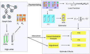
Figure 3: The workflow of our gDIS model for estimating PDE, PIE and STE within network data.

Using attention weights to capture the varying influences of nodes.

A two-layer GNN with attention mechanisms dynamically weights the importance o neighboring nodes when updating each node’s representation. By considering both direct and second-order neighbors, we calculate the attention coefficients $\alpha_{ij}$ to indicate the relative importance of each neighbor as follows:

$$\alpha_{ij}=\frac{\exp(\phi({\mathbf{A}}^{T}[\mathbf{W}\mathbf{H}_{i}\,||\,\mathbf{W}\mathbf{H}_{j}]))}{\sum_{k\in\mathcal{N}(i)\cup\{i\}}\exp(\phi({\mathbf{A}}^{T}[\mathbf{W}\mathbf{H}_{i}\,||\,\mathbf{W}\mathbf{H}_{k}]))}$$ (13)

where $\alpha_{ij}$ indicates the importance of neighfbor $j$ to node $i$, and $\phi(\cdot)$ is the LeakyReLU activation function (Xu et al. 2020). ${\mathbf{A}}$ is a learnable weight vector used to calculate the unnormalized attention score between nodes, while $\mathbf{W}$ is a learnable weight matrix that linearly transforms the feature vector $\mathbf{H}$. $\mathbf{H}_{i}$ and $\mathbf{H}_{j}$ are the feature vectors of nodes $i$ and $j$, respectively, and $||$ denotes vector concatenation. $\mathcal{N}(i)$ represents the neighbor set of node $i$.

The new feature representation of node $i$ incorporates both its own information and that of its neighbors, resulting in a more comprehensive and accurate update.

$$H^{\prime}_{i}=\sigma(\sum_{j\in\mathcal{N}(i)\cup\{i\}}\alpha_{ij}\mathbf{W}\mathbf{H}_{j})$$ (14)

where $\sigma(\cdot)$ represents the ELU activation function (Ide and Kurita 2017).

HSIC Regularization.

HSIC (Ahmad, Mazzara, and Distefano 2021) measures the dependence between two variables in a Reproducing Kernel Hilbert Space (RKHS) (Berlinet and Thomas-Agnan 2011). Adding an HSIC regularization term to the loss function promotes independence between the original features and node embeddings, encouraging the embeddings to rely more on graph structure rather than node features, thereby reducing overfitting and improving robustness.

The feature matrix $\mathbf{H}$ and the kernel matrix $\mathbf{H}^{\prime}$ using the Gaussian kernel (Keerthi and Lin 2003) function are defined as follows:

$$(\mathbf{K}_{\mathbf{H}})_{il}=\exp\left(-\frac{\|\mathbf{H}_{i}-\mathbf{H}_{l}\|^{2}}{2\gamma^{2}}\right)$$ (15)

$$(\mathbf{K}_{\mathbf{H}^{\prime}})_{il}=\exp\left(-\frac{\|\mathbf{H}^{\prime}_{i}-\mathbf{H}^{\prime}_{l}\|^{2}}{2\gamma^{2}}\right)$$ (16)

where $\|\mathbf{H}_{i}-\mathbf{H}_{l}\|^{2}$ is the squared euclidean distance (Danielsson 1980) between feature vectors $\mathbf{H}_{i}$ and $\mathbf{H}_{l}$. $\gamma$ is the Gaussian kernel bandwidth (Kakde et al. 2017), set to the median of input feature distances. $\mathbf{I}$ is the $m\times m$ identity matrix, $\mathbf{1}$ is an $m\times 1$ vector of ones, and $m$ is the total number of samples. The centering matrix $\mathbf{C}$ is calculated as:

$$\mathbf{C}=\mathbf{I}-\frac{1}{n}\mathbf{1}\mathbf{1}^{T}$$ (17)

Objective Function.

We use mean squared error (MSE) loss (Chicco, Warrens, and Jurman 2021) to measure the difference between actual and predicted values. Our final objective function is:

$$\mathcal{L}_{\text{total}} =\frac{1}{n}\sum_{i=1}^{n}(Y_{i}-\hat{Y}_{i})^{2}$$ (18)

$$+\lambda\cdot\frac{1}{(n-1)^{2}}\text{trace}(\mathbf{K}_{\mathbf{H}}\mathbf{C}\mathbf{K}_{\mathbf{H}^{\prime}}\mathbf{C})$$

where $\lambda$ is a hyperparameter set to 0.1. The trace term measures the dependence between the feature matrix $\mathbf{H}$ and the embedding matrix $\mathbf{H}^{\prime}$.

Experiments

In this section, we evaluate the causal effect estimation capabilities of gDIS. We use standard evaluation metrics to compare the performance of gDIS against baseline models, validating its effectiveness.

Experiments Setup

Datasets. Each unit $i$ has only one observed treatment $T_{i}$, peer exposure $Z_{i}$, and outcome $Y_{i}$ (the factual outcome), making direct causal effect estimation challenging due to unobservable counterfactuals. Following (Jiang and Sun 2022; Chen et al. 2024), we use semi-synthetic datasets where the network structure (features and link) is real, but treatments and outcomes are simulated. The datasets include two real-world social networks: BlogCatalog and Flickr (Li et al. 2015), with detailed descriptions provided in the Appendix.

Given the high-dimensional and sparse nature of the original features, we follow the approach in (Jiang and Sun 2022; Chen et al. 2024) and apply Latent Dirichlet Allocation (LDA) (Blei, Ng, and Jordan 2003) to reduce the dimension to 10. The network is then divided into training, validation, and test sets using the METIS algorithm (Karypis and Kumar 1998). $T$ and $Y$ are simulated according to the procedure outlined in Fig. 2(a). Due to space limitations, further details are provided in the appendix.

Data	Effects	CFR(+N)	ND(+N)	TARNET(+N)	NetEst	TNet	gDIS(-HSIC)	gDIS
BC (within-sample)	peer	0.3195±0.0299	0.3488±0.0249	0.2830±0.0229	0.0890±0.0252	0.1019±0.0275	0.0750±0.0224	0.0719±0.0062
	peer direct	/	/	/	/	/	0.0514±0.0121	0.0487±0.0092
	peer indirect	/	/	/	/	/	0.0236±0.0110	0.0232±0.0056
	self-treatment	0.5929±0.0565	0.5571±0.0855	0.4922±0.0522	0.3322±0.0461	0.2671±0.1372	0.1973±0.0800	0.1816±0.0020
BC (out-of-sample)	peer	0.3184±0.0259	0.3488±0.0250	0.2898±0.0263	0.1198±0.0279	0.0984±0.0248	0.0791±0.0081	0.0628±0.0090
	peer direct	/	/	/	/	/	0.0422±0.0091	0.0364±0.0121
	peer indirect	/	/	/	/	/	0.0369±0.0052	0.0264±0.0048
	self-treatment	0.5913±0.0559	0.5478±0.0810	0.5611±0.1431	0.2856±0.0407	0.2653±0.1253	0.1763±0.0111	0.1738±0.0126
Flickr (within-sample)	peer	0.2575±0.0741	0.3011±0.0651	0.2215±0.0585	0.0917±0.0072	0.1209±0.0450	0.0771±0.0177	0.0565±0.0175
	peer direct	/	/	/	/	/	0.0456±0.0093	0.0290±0.0109
	peer indirect	/	/	/	/	/	0.0315±0.0144	0.0275±0.0095
	self-treatment	0.2939±0.0984	0.2896±0.1077	0.2316±0.0715	0.0772±0.0118	0.2875±0.1912	0.1734±0.0114	0.1619±0.0165
Flickr (out-of-sample)	peer	0.2646±0.0732	0.3112±0.0501	0.2237±0.0588	0.0911±0.0075	0.1216±0.0730	0.0793±0.0180	0.0550±0.0196
	peer direct	/	/	/	/	/	0.0458±0.0081	0.0282±0.0121
	peer indirect	/	/	/	/	/	0.0335±0.0148	0.0268±0.0098
	self-treatment	0.2973±0.0918	0.2903±0.1079	0.2255±0.0599	0.0808±0.0121	0.2977±0.1883	0.1882±0.0115	0.1474±0.0158

Table 2: Causal effect estimation results. The $\epsilon_{PEHE}$ error is reported. The top-performing results are emphasized in bold. Note that “/” indicates the model is not applicable for this effect.

Metrics.

We evaluate the algorithms using two metrics: MSE (Chicco, Warrens, and Jurman 2021) and PEHE (Grimmer, Messing, and Westwood 2017). MSE, defined as $\epsilon_{MSE}=\frac{1}{m}\sum_{i=1}^{m}(\hat{Y}_{i}-Y_{i})^{2}$, measures counterfactual estimation accuracy. PEHE, defined as $\epsilon_{PEHE}=\sqrt{\frac{1}{m}\sum_{i=1}^{m}\left[(\hat{Y}_{i}(t^{\prime})-\hat{Y}_{i}(t))-(Y_{i}(t^{\prime})-Y_{i}(t))\right]^{2}}$, evaluates the precision in estimating heterogeneous effects. Here, $\hat{Y}_{i}$ and $Y_{i}$ denote estimated and ground truth outcomes, with lower values indicating better performance.

Baselines.

We compared our model with six baselines: (1) CFR (Shalit, Johansson, and Sontag 2017), the state-of-the-art for effect estimation on IID data using integral probability metrics (IPM) for distribution balancing; (2) TARNet (Shalit, Johansson, and Sontag 2017), a variant of CFR without IPM; (3) NetDeconf (Guo, Li, and Liu 2020), an adaptation of CFR for network data using GNNs to encode confounders; CFR+(N), TARNet+(N), NetDeconf+(N), which add peer exposure to handle network interference; (4) NetEst (Jiang and Sun 2022), which applies adversarial learning to bridge graph ML and causal effect estimation; (5) TNet (Chen et al. 2024), integrating target learning; (6) gDIS (-HSIC), our gDIS method without the HSIC module.

Implementation Details.

We use a 2-layer GNN with attention mechanisms and a 3-layer fully connected estimator, with hidden embeddings of size 32. The learning rate is set to 0.001 for all modules, and the Adam optimizer (Zhang 2018) is used. Each task is repeated five times, with average results and standard deviations reported. Experiments are conducted using PyTorch 1.7.0, Python 3.8, CUDA 11.0, on an RTX A4000 GPU (16GB), 12 vCPUs (Xeon Gold 5320 @ 2.20GHz), 32GB memory, and Windows OS.

Results.

Our gDIS model estimates PDE, PIE, total peer effects (sum of peer direct and indirect effects), and self-treatment effects at the group level. We evaluate “within-sample” estimates on training networks and “out-of-sample” estimates on testing networks. Table 2 summarizes the $\epsilon_{PEHE}$ results on the BC and Flickr datasets. gDIS consistently outperforms baseline models in both settings, indicating that our objective function effectively reduces counterfactual prediction errors. Moreover, the HSIC module significantly improves performance on the test set, demonstrating greater effectiveness and robustness compared to other models. While baseline models estimate total peer effects, they fail to distinguish between direct and indirect effects.

In our counterfactual experiments, following (Jiang and Sun 2022), we simulated outcomes by varying the treatment flip rate (0.25, 0.5, 0.75, 1). As shown in Fig 4, higher flip rates generally lead to increased MSE, except in the case of the gDIS model under the “Flickr out-of-sample” setting, where the error remains stable, underscoring the HSIC module’s role in improving generalization. Additionally, the Flickr dataset typically exhibits higher MSE compared to BC, likely due to its larger number of edge relationships.

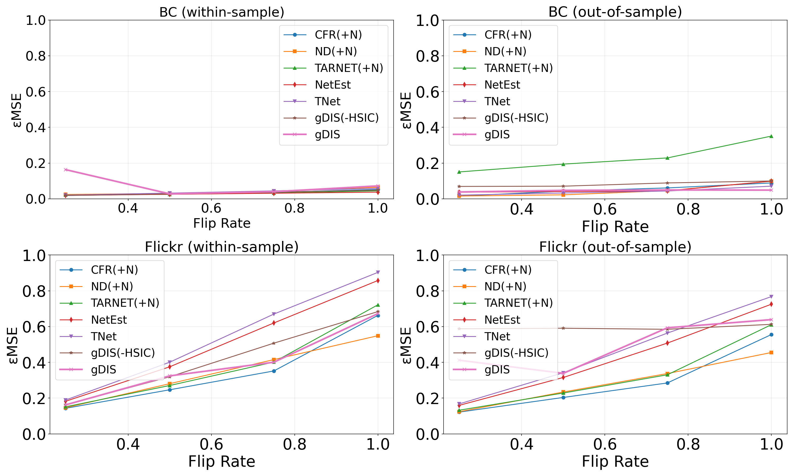
Figure 4: The results illustrate the relationship between the counterfactual estimation error ($\epsilon_{MSE}$) and the percentage of units with treatment flip.

Related Work

In this section, we review methods for estimating causal effects in network data that are related to our gDIS method.

Estimating Peer Effects in Network Data.

There are various methods for estimating peer effects in network data, where interference arises when an individual’s treatment influences the outcomes of connected individuals. For example, Forastiere et al. (Forastiere, Airoldi, and Mealli 2021) addressed this issue with a covariate adjustment method using a generalized propensity score (PS) (Feng et al. 2012) to balance both individual and neighborhood covariates. Jiang et al. (Jiang and Sun 2022) introduced NetEst, a framework that employs graph neural networks (GNNs) to capture feature representations of both individual nodes and their first-order neighbors. Cai et al. (Cai et al. 2023) expanded on this by deriving generalization bounds and proposing a joint propensity score approach combined with representation learning via weighted regression. Ma et al. (Ma et al. 2022) developed HyperSCI, which leverages hypergraph neural networks (HGNNs) (Ma et al. 2022) to model interference using a multilayer perceptron (MLP) (Popescu et al. 2009) and hypergraph convolution. However, none of these methods distinguish between direct and indirect peer effects.

Estimating Peer Direct and Indirect Effects in Network Data.

Another line of research focuses on estimating both direct and indirect peer effects in network data. VanderWeele et al. (VanderWeele, Tchetgen, and Halloran 2012) examined the effects of vaccination in small family units, such as the impact of a child’s vaccination on the mother. Shpitser et al. (Shpitser, Tchetgen, and Andrews 2017) developed a chain graph-based method to decompose peer effects into unit-specific components. Cai et al. (Cai, Loh, and Crawford 2021) evaluated contagion, susceptibility, and infectiousness effects in symmetric partnerships under infectious disease settings. Ogburn et al. (Ogburn et al. 2024) analyzed obesity status in the Framingham Heart Study using longitudinal logistic regression, noting potential issues with dependence and model misspecification. However, these studies generally focus on scenarios with a propagation unit size of two, which may limit practical applicability. Ogburn et al. (Ogburn, Shpitser, and Lee 2020) also used a log-linear model within the chain graph framework to evaluate the decisions of nine judges. However, the assumption of system equilibrium may not hold in dynamic environments, limiting the model’s accuracy and applicability. Different from these reviewed works, our work focus on estimating peer direct and indirect effects at the group level. This more generalized setting allows us to capture the collective influence of groups, which is crucial for informing intervention strategies.

Conclusion

Summary of Contributions. In this work, we address the novel problem of estimating three types of causal effects in observational network data by proposing a new method, gDIS. Our approach differentiates between group-level PDE, PIE, and STE in observational network data. Through theoretical analysis, we establish identifiability conditions and provide corresponding proofs for the identifiability of these causal effects. To capture complex network interactions, gDIS employs a multi-layer GNN with attention mechanisms and incorporate HSIC to effectively control dependencies between node features. We validated the effectiveness and robustness of our gDIS on two semi-synthetic datasets, demonstrating strong performance even in complex network environments.

Limitations & Future Work. While our framework is supported by theorems and the performance of gDIS has been demonstrated, there are limitations. Our approach relies on the network unconfoundedness assumption, which may be violated in practice, despite being common in the literature. In future work, we aim to relax these assumptions to expand the applicability of our method.

References

- Ahmad, Mazzara, and Distefano (2021) Ahmad, M.; Mazzara, M.; and Distefano, S. 2021. Regularized CNN feature hierarchy for hyperspectral image classification. Remote Sensing, 13(12): 2275.
- Belov and Armstrong (2011) Belov, D. I.; and Armstrong, R. D. 2011. Distributions of the Kullback–Leibler divergence with applications. British Journal of Mathematical and Statistical Psychology, 64(2): 291–309.
- Berlinet and Thomas-Agnan (2011) Berlinet, A.; and Thomas-Agnan, C. 2011. Reproducing kernel Hilbert spaces in probability and statistics. Springer Science & Business Media.
- Blei, Ng, and Jordan (2003) Blei, D. M.; Ng, A. Y.; and Jordan, M. I. 2003. Latent dirichlet allocation. Journal of machine Learning research, 3(Jan): 993–1022.
- Cai et al. (2023) Cai, R.; Yang, Z.; Chen, W.; Yan, Y.; and Hao, Z. 2023. Generalization bound for estimating causal effects from observational network data. In Proceedings of the 32nd ACM International Conference on Information and Knowledge Management, 163–172.
- Cai, Loh, and Crawford (2021) Cai, X.; Loh, W. W.; and Crawford, F. W. 2021. Identification of causal intervention effects under contagion. Journal of causal inference, 9(1): 9–38.
- Chen et al. (2024) Chen, W.; Cai, R.; Yang, Z.; Qiao, J.; Yan, Y.; Li, Z.; and Hao, Z. 2024. Doubly Robust Causal Effect Estimation under Networked Interference via Targeted Learning. arXiv preprint arXiv:2405.03342.
- Chicco, Warrens, and Jurman (2021) Chicco, D.; Warrens, M. J.; and Jurman, G. 2021. The coefficient of determination R-squared is more informative than SMAPE, MAE, MAPE, MSE and RMSE in regression analysis evaluation. Peerj computer science, 7: e623.
- Danielsson (1980) Danielsson, P.-E. 1980. Euclidean distance mapping. Computer Graphics and image processing, 14(3): 227–248.
- Feng et al. (2012) Feng, P.; Zhou, X.-H.; Zou, Q.-M.; Fan, M.-Y.; and Li, X.-S. 2012. Generalized propensity score for estimating the average treatment effect of multiple treatments. Statistics in Medicine, 31(7): 681–697.
- Forastiere, Airoldi, and Mealli (2021) Forastiere, L.; Airoldi, E. M.; and Mealli, F. 2021. Identification and estimation of treatment and interference effects in observational studies on networks. Journal of the American Statistical Association, 116(534): 901–918.
- Grimmer, Messing, and Westwood (2017) Grimmer, J.; Messing, S.; and Westwood, S. J. 2017. Estimating heterogeneous treatment effects and the effects of heterogeneous treatments with ensemble methods. Political Analysis, 25(4): 413–434.
- Guo, Li, and Liu (2020) Guo, R.; Li, J.; and Liu, H. 2020. Learning individual causal effects from networked observational data. In Proceedings of the 13th international conference on web search and data mining, 232–240.
- Hu et al. (2020) Hu, Z.; Dong, Y.; Wang, K.; Chang, K.-W.; and Sun, Y. 2020. Gpt-gnn: Generative pre-training of graph neural networks. In Proceedings of the 26th ACM SIGKDD international conference on knowledge discovery & data mining, 1857–1867.
- Ide and Kurita (2017) Ide, H.; and Kurita, T. 2017. Improvement of learning for CNN with ReLU activation by sparse regularization. In 2017 international joint conference on neural networks (IJCNN), 2684–2691. IEEE.
- Imai, Keele, and Yamamoto (2010) Imai, K.; Keele, L.; and Yamamoto, T. 2010. Identification, inference and sensitivity analysis for causal mediation effects. Statistical Science, 25(1): 51 – 71.
- Imbens and Rubin (2010) Imbens, G. W.; and Rubin, D. B. 2010. Rubin causal model. In Microeconometrics, 229–241. Springer.
- Jiang and Sun (2022) Jiang, S.; and Sun, Y. 2022. Estimating causal effects on networked observational data via representation learning. In Proceedings of the 31st ACM International Conference on Information & Knowledge Management, 852–861.
- Kakde et al. (2017) Kakde, D.; Chaudhuri, A.; Kong, S.; Jahja, M.; Jiang, H.; and Silva, J. 2017. Peak criterion for choosing Gaussian kernel bandwidth in support vector data description. In 2017 IEEE International Conference on Prognostics and Health Management (ICPHM), 32–39. IEEE.
- Karypis and Kumar (1998) Karypis, G.; and Kumar, V. 1998. A fast and high quality multilevel scheme for partitioning irregular graphs. SIAM Journal on scientific Computing, 20(1): 359–392.
- Keerthi and Lin (2003) Keerthi, S. S.; and Lin, C.-J. 2003. Asymptotic behaviors of support vector machines with Gaussian kernel. Neural computation, 15(7): 1667–1689.
- Lee, Lessler, and Stuart (2010) Lee, B. K.; Lessler, J.; and Stuart, E. A. 2010. Improving propensity score weighting using machine learning. Statistics in medicine, 29(3): 337–346.
- Li et al. (2015) Li, J.; Hu, X.; Tang, J.; and Liu, H. 2015. Unsupervised streaming feature selection in social media. In Proceedings of the 24th ACM International on Conference on Information and Knowledge Management, 1041–1050.
- Ma et al. (2022) Ma, J.; Wan, M.; Yang, L.; Li, J.; Hecht, B.; and Teevan, J. 2022. Learning causal effects on hypergraphs. In Proceedings of the 28th ACM SIGKDD Conference on Knowledge Discovery and Data Mining, 1202–1212.
- MacKinnon, Fairchild, and Fritz (2007) MacKinnon, D. P.; Fairchild, A. J.; and Fritz, M. S. 2007. Mediation analysis. Annu. Rev. Psychol., 58: 593–614.
- Niu, Zhong, and Yu (2021) Niu, Z.; Zhong, G.; and Yu, H. 2021. A review on the attention mechanism of deep learning. Neurocomputing, 452: 48–62.
- Ogburn, Shpitser, and Lee (2020) Ogburn, E. L.; Shpitser, I.; and Lee, Y. 2020. Causal inference, social networks and chain graphs. Journal of the Royal Statistical Society Series A: Statistics in Society, 183(4): 1659–1676.
- Ogburn et al. (2024) Ogburn, E. L.; Sofrygin, O.; Diaz, I.; and Van der Laan, M. J. 2024. Causal inference for social network data. Journal of the American Statistical Association, 119(545): 597–611.
- Pearl (2009) Pearl, J. 2009. Causality. Cambridge University Press.
- Pearl (2014) Pearl, J. 2014. Interpretation and identification of causal mediation. Psychological methods, 19(4): 459.
- Popescu et al. (2009) Popescu, M.-C.; Balas, V. E.; Perescu-Popescu, L.; and Mastorakis, N. 2009. Multilayer perceptron and neural networks. WSEAS Transactions on Circuits and Systems, 8(7): 579–588.
- Shalit, Johansson, and Sontag (2017) Shalit, U.; Johansson, F. D.; and Sontag, D. 2017. Estimating individual treatment effect: generalization bounds and algorithms. In International conference on machine learning, 3076–3085. PMLR.
- Shpitser, Tchetgen, and Andrews (2017) Shpitser, I.; Tchetgen, E. T.; and Andrews, R. 2017. Modeling Interference Via Symmetric Treatment Decomposition. arXiv: Methodology.
- Sinclair, McConnell, and Green (2012) Sinclair, B.; McConnell, M.; and Green, D. P. 2012. Detecting spillover effects: Design and analysis of multilevel experiments. American Journal of Political Science, 56(4): 1055–1069.
- Van der Laan, Rose et al. (2011) Van der Laan, M. J.; Rose, S.; et al. 2011. Targeted learning: causal inference for observational and experimental data, volume 4. Springer.
- VanderWeele, Tchetgen, and Halloran (2012) VanderWeele, T. J.; Tchetgen, E. J. T.; and Halloran, M. E. 2012. Components of the indirect effect in vaccine trials: identification of contagion and infectiousness effects. Epidemiology, 23(5): 751–761.
- Xu et al. (2020) Xu, J.; Li, Z.; Du, B.; Zhang, M.; and Liu, J. 2020. Reluplex made more practical: Leaky ReLU. In 2020 IEEE Symposium on Computers and communications (ISCC), 1–7. IEEE.
- Yao et al. (2021) Yao, L.; Chu, Z.; Li, S.; Li, Y.; Gao, J.; and Zhang, A. 2021. A survey on causal inference. ACM Transactions on Knowledge Discovery from Data (TKDD), 15(5): 1–46.
- Zhang (2018) Zhang, Z. 2018. Improved adam optimizer for deep neural networks. In 2018 IEEE/ACM 26th international symposium on quality of service (IWQoS), 1–2. Ieee.