How to use the dispersion in the tensor for broadband generation of polarization-entangled photons
Abstract
Polarization-entangled photon pairs are a widely used resource in quantum optics and technologies, and are often produced using a nonlinear process. Most sources based on spontaneous parametric downconversion have relatively narrow optical bandwidth because the pump, signal and idler frequencies must satisfy a phase-matching condition. Extending the bandwidth, for example to achieve spectral multiplexing, requires changing some experimental parameters such as temperature, crystal angle, poling period, etc. Here, we demonstrate broadband (tens of THz for each photon) generation of polarization-entangled photon pairs by spontaneous four-wave mixing in a diamond crystal, with a simple colinear geometry requiring no further optical engineering. Our approach leverages the quantum interference between electronic and vibrational contributions to the tensor. Entanglement is characterized in a single realization of a Bell test over the entire bandwidth using fiber dispersion spectroscopy and fast single-photon detectors. The results agree with the biphoton wavefunction predicted from the knowledge of the and Raman tensors and demonstrate the general applicability of our approach to other crystalline materials.
Introduction.— Nonlinear optical processes play a pivotal role in producing and engineering quantum states of light. Spontaneous parametric-down conversion (PDC) and four-wave mixing (FWM), which rely respectively on the and susceptibility of materials, have been employed for generating a variety of photonic quantum states [1] – entangled photon pairs generated in the low-gain regime being the most popular class. PDC sources generally offer the highest brightness because, for non-centrosymmetric crystals, is much larger than . A challenge with PDC is the large frequency difference between the pump and the signal/idler fields that restricts the spectral bandwidth over which phase matching can be achieved without modifying the experimental conditions or implementing delicate dispersion engineering in periodically poled waveguides [2]. Moreover, materials such as silicon and diamond have no nonlinearity while being popular platforms for integrated quantum photonics at telecom and visible wavelengths, respectively [3]; it motivates the use of FWM for generating entangled photons.
Among the photonic degrees of freedom that can be entangled, polarization is often the easiest to manipulate and measure. However, generating polarization entanglement usually requires careful engineering of the source, since parametric nonlinear processes more naturally generate photon pairs that are entangled in the temporal and spatial degrees of freedom due to energy and momentum conservation, respectively. There are relatively few demonstrations of polarization-entangled photon pair produced by spontaneous FWM, with the most established methods relying on the nonlinearity of optical fibers [4, 5, 6, 7] or silicon waveguides [8] that are themselves embedded within a Sagnac loop. The photon pairs produced by FWM in glass fibers or silicon waveguides are typically copolarized, so that entanglement is generated from two orthogonal sources after erasing distinguishing information in all other degrees of freedom (spatial and temporal). This erasure has also been achieved using a fully-integrated silicon photonic circuit comprising a polarization rotator between TE and TM modes [9]. In an effort to simplify such FWM sources, researchers leveraged the tensorial nature of the nonlinear response and engineered the polarization mode dispersion to achieve polarization entanglement directly out of silicon [10] and AlGaAs [11] waveguides.
When FWM is used to generate photon pairs, vibrational Raman scattering is mostly known as a source of noise degrading the purity of the joint quantum state [12]. This problem is particularly pronounced in amorphous media such as optical fibers because the Raman scattered light has a broad spectrum [13]. In crystalline materials such as silicon, AlGaAs and diamond, the Raman peak is very sharp (few wavenumbers), so that Raman noise is more easily avoided by choosing an appropriate detuning from the pump. Interestingly, a recent work by Freitas et al. showed that polarization entanglement can be generated from bulk diamond for pairs detuned by from the degenerate two-photon pump [14], a result qualitatively attributed to the interference of electronic and vibrational (Raman) microscopic pathways leading to photon pair creation.
In this Letter, we establish a theory of polarization-entangled photon pair generation using FWM in diamond (also applicable to silicon and other crystals for which the and Raman tensors are known) and validate our predictions by performing coincidence measurements and Bell tests over a large optical bandwidth of ( THz) on either side of the pump frequency (spanning 130 THz in total). Moreover, we achieve this characterization in a single set of polarization measurements by employing fiber spectroscopy [15], where the frequency information of individual photons is mapped onto detection time through the natural dispersion of optical fibers. The relaxed phase-matching condition for FWM enables statistically significant violation of the CHSH inequality [16] for the Bell state across a considerable bandwidth, at all measured frequency shifts below ( THz) – a bandwidth on par with that of state-of-the-art single-photon sources in optimized photonic platforms [17, 18]. We find that our results agree with the theoretical predictions accounting for the frequency dependence of that is due to the sharp vibrational Raman resonance at .
We notice that the term “broadband” is sometimes used in the literature to indicate correlated photon-pair sources capable of establishing entanglement between far-detuned photons – typically to bridge visible and telecom ranges – while keeping a narrow linewidth [19]. On the contrary, we generate a broad bandwidth of entangled photon pairs at once with a single pump laser of fixed frequency. In this sense, our technique also offers an advantage over coherent anti-Stokes Raman scattering (CARS) for probing third-order nonlinearities. Indeed, the dispersion features we analyze could be obtained with CARS only by employing an additional broadly tunable ( nm) visible pump. In analogy to CARS, a recent work [20] used a tunable THz source to evidence third-harmonic enhancement and suppression in diamond, qualitatively explained in terms of the same dispersion.
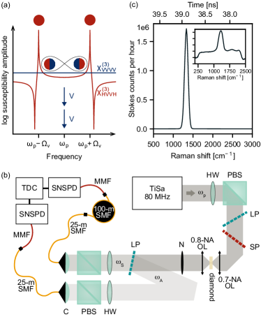
Results.— Figure 1a illustrates the concept of the experiment in the frequency domain. Two vertically-polarized pump photons at frequency can generate pairs of correlated photon pairs at (Stokes) and (anti-Stokes) frequencies, satisfying energy conservation. The polarization state of the correlated pair is determined by the third-order susceptibility tensor of diamond, as we will explicate below. Quite generally, the existence of a Raman-active optical phonon mode at frequency causes a resonant contribution to the tensor when photon pairs satisfy [21]. The aim of this article is to show how these intrinsic material properties can be used to produce polarization-entangled photons over a large bandwidth around without any further optical engineering. Our results are therefore applicable to other crystalline materials.
Figure 1b shows the experimental setup. A mode-locked Titanium:Sapphire oscillator (Tsunami, Spectra Physics) generates -fs pulses at nm with a repetition rate of MHz. In order to resolve the sharp spectral dependence of the susceptibility sketched in Fig. 1a, the pump pulse duration should be of the same order of magnitude as the phonon coherence time, which is around 8 ps in diamond [22]. We use tunable long-pass (LP) and short-pass (SP) filters to increase the pulse duration to ps by reducing the spectral width to nm. The average power on the sample is mW (600 pJ pulse energy), below the onset of single-beam stimulated processes [23].
The collected Stokes and anti-Stokes signals are split into two different paths by a longpass interference filter placed almost perpendicular to the beam to minimize the polarization-dependent response between and components. Next, each signal is spectrally dispersed through m of single-mode fibers (SMFs). Since losses also increase with the fiber length, we add m SMF only to the Stokes path. Knowing the dispersion parameters of the fibers, we can convert photon detection times into detuning from the pump in wavenumbers [24]. Superconducting nanowire single-photon detectors (SNSPDs) allow us to achieve a temporal resolution of around ps per detector (time jitter). Figure 1c shows the Stokes spectrum obtained the laser synchronization pulse is used as the start signal and the detection of a polarized Stokes photon as the stop signal.
Fiber spectroscopy had been employed to measure various spectral properties of photon pairs generated by PDC, like the joint spectral amplitude [25] and the second-order correlation function [26]. Ref. [27] measured the spectrum of PDC-generated polarization-entangled photons, but the spectral variation of the quantum state was not addressed. Our work reveals the frequency evolution of the degree of purity, polarization entanglement, and non-locality of the biphoton state generated by FWM. Our measurement technique can also be used to characterize novel sources of polarization-entangled photons implemented in flat optical systems [28, 29, 30], including metamaterials [31, 32] and nanoresonators [33, 34].
Since diamond is centrosymmetric, the third-order susceptibility mediates the lowest-order nonlinear optical processes. It is a complex rank-3 tensor that depends of the frequencies and polarizations of the four fields involved: , where the indices specify the polarization directions of the fields at the four frequencies listed in the same order in the parenthesis. In a stimulated scattering experiment, two incoming beams at and can generate light at through the following third-order nonlinear processes: (i) stimulated Raman scattering, when , which is the optical phonon frequency (ii) two-photon absorption, when corresponds to an electronic transition, and (iii) any non-resonant FWM process mediated by far-detuned electronic levels. In 1974, Levenson and Bloembergen performed stimulated FWM spectroscopy on diamond and from the independent knowledge of the Raman tensor and Raman gain they extracted all components of its tensor [35].
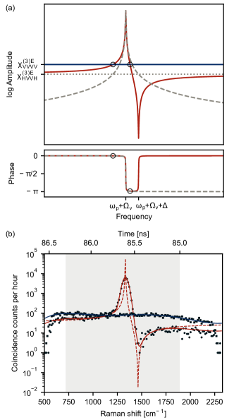
In our experiment, we employ a single pump beam with frequency far from any electronic resonance. We can therefore neglect two-photon absorption and write where is the non-resonant – hence real – electronic FWM contribution and is the (complex) vibrational Raman scattering contribution featuring a resonance at , [21] where is the frequency of the optical phonon at . The pump propagates along the [100] crystallographic axis and the diamond is rotated to align the [001] axis with the pump polarization, which is vertical in the laboratory frame [24]. In this configuration, Raman scattering () only generates horizontally polarized pairs [35, 14]. Figure 2a shows the amplitude and phase of the non-zero components of the susceptibility tensor contributing in this case
| (1) | ||||
| (2) |
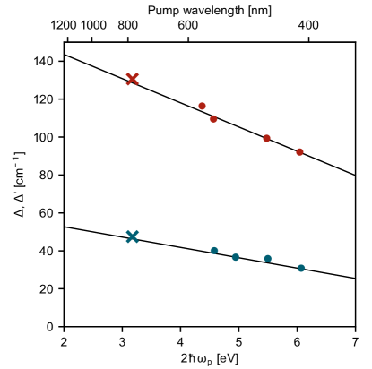
where , and is the vibrational decay rate with the Raman linewidth. Following Ref.[35], we define , where is proportional to the Raman tensor and is the volumic density of unit cells. The value of corresponds to the angular frequency difference between the maximum and minimum of , i.e. between the points of maximum constructive and destructive interference of and (Fig. 2).
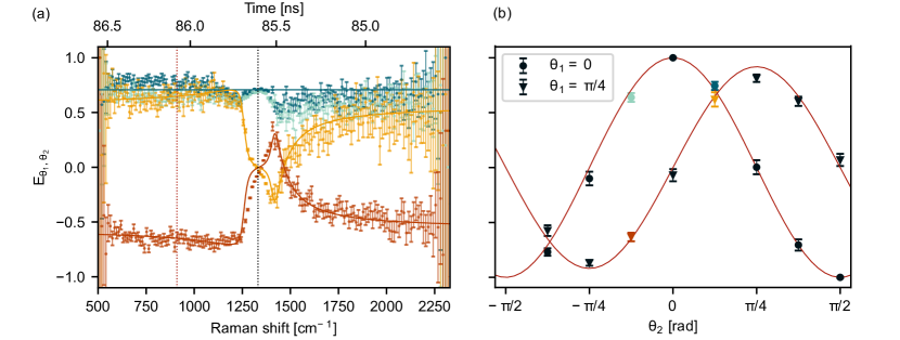
The measured rate of photon pairs for and polarizations follow the proportionality relations and , respectively. We measure them by counting the coincidences between anti-Stokes and Stokes photons after they pass through parallel polarizers, as displayed in Fig. 2b. Since is theoretically constant in frequency, we use the measured as a characterization of the setup spectral response, which we assume polarization independent (the polarization of photons is largely scrambled by the time they impinge on the SNSPD). To account for the spectral broadening due to the finite pump bandwidth and the temporal jitter of the detectors, the theoretical -polarized intensity is convoluted with a Gaussian of variance centered at . After multiplying by the setup response extracted above, the resulting model (red line in Fig. 2b) accurately reproduces our data.

In the End Matter, we give the general biphoton polarization state generated under arbitrary pump polarization. For a vertical pump polarization the wavefunction reduces to
| (3) |
As customary for spontaneous PDC and FWM in the low gain regime, this biphoton wavefunction should be understood as the one-photon-pair component of the full two-mode squeezed state. It is an excellent description of the results obtained by coincidence measurements (which are not sensitive to the vacuum component) as long as the probability of photon pair emission is much smaller than one per pulse so that double-pair emission is a negligible process. The probability to measure a coincidence when Stokes and anti-Stokes polarizers are set at angles and is expressed in the End Matter; from Eq. 11 we extract the correlation parameter and the CHSH parameters [16]
| (4) |
where . The corresponding Bell inequalities are maximally violated by the Bell states
| (5) |
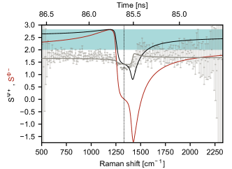
respectively. As shown in Figures 3a-b, we extract the parameters for from the direct measurement of and compare them with the values theoretically computed from Equations 12-4 with and fixed by the measurement of and in Fig. 2b. The parameter is set to to best reproduce the data within a range of values constrained by the material’s anisotropy [24]. The measured and theoretical values demonstrate a good agreement. The Bell inequality for is violated by up to standard deviations over a broad spectral range below 1250 cm-1. The measured and theoretical values of display no violation of the corresponding Bell inequality. This is a consequence of the sub-optimal spectral resolution of the measurement. In the ideal case, before the convolution with the Gaussian (dashed black curve), the inequality is violated in a narrow spectral region around , where the biphoton state is .
Discussion.— In our experiment, the coincidence detection rate of polarization-entangled photon pairs per unit bandwidth is of Hz/nm for a pump power of mW, with an overall detection efficiency not better than a few percent (including total internal reflection inside the diamond, fiber coupling losses, propagation losses and detector efficiency). The pair generation rate is therefore on the order of 10 Hz/nm for an interaction length of m determined by the depth of focus. How much could the brightness of the source be improved? As detailed in the End Matter, based on the results from Ref. 36, we estimate that a centimeter-long diamond waveguide pumped under similar conditions would generate pairs at rate of 10 to 100 kHz/nm, which would further increase quadratically with pump power and be enhanced using photonic resonators. Our results therefore motivate further development of diamond photonic integrated circuits tailored to produce broadband polarization entangled photons around any center wavelength in the material’s transparency window.
Data availability statement
The data that support the findings of this study will be deposited in a Zenodo repository with DOI…
Code availability statement
The code used in this study for data analysis and modeling will be deposited in a Zenodo repository with DOI…
References
- Wang et al. [2021] Y. Wang, K. D. Jöns, and Z. Sun, Integrated photon-pair sources with nonlinear optics, Applied Physics Reviews 8, 011314 (2021).
- Javid et al. [2021] U. A. Javid, J. Ling, J. Staffa, M. Li, Y. He, and Q. Lin, Ultrabroadband entangled photons on a nanophotonic chip, Phys. Rev. Lett. 127, 183601 (2021).
- Moody et al. [2022] G. Moody, V. J. Sorger, D. J. Blumenthal, P. W. Juodawlkis, W. Loh, C. Sorace-Agaskar, A. E. Jones, K. C. Balram, J. C. F. Matthews, A. Laing, M. Davanco, L. Chang, J. E. Bowers, N. Quack, C. Galland, I. Aharonovich, M. A. Wolff, C. Schuck, N. Sinclair, M. Lončar, T. Komljenovic, D. Weld, S. Mookherjea, S. Buckley, M. Radulaski, S. Reitzenstein, B. Pingault, B. Machielse, D. Mukhopadhyay, A. Akimov, A. Zheltikov, G. S. Agarwal, K. Srinivasan, J. Lu, H. X. Tang, W. Jiang, T. P. McKenna, A. H. Safavi-Naeini, S. Steinhauer, A. W. Elshaari, V. Zwiller, P. S. Davids, N. Martinez, M. Gehl, J. Chiaverini, K. K. Mehta, J. Romero, N. B. Lingaraju, A. M. Weiner, D. Peace, R. Cernansky, M. Lobino, E. Diamanti, L. T. Vidarte, and R. M. Camacho, 2022 roadmap on integrated quantum photonics, Journal of Physics: Photonics 4, 012501 (2022).
- Takesue and Inoue [2004] H. Takesue and K. Inoue, Generation of polarization-entangled photon pairs and violation of bell’s inequality using spontaneous four-wave mixing in a fiber loop, Phys. Rev. A 70, 031802 (2004).
- Li et al. [2005] X. Li, P. L. Voss, J. E. Sharping, and P. Kumar, Optical-fiber source of polarization-entangled photons in the 1550 nm telecom band, Phys. Rev. Lett. 94, 053601 (2005).
- Fan et al. [2007] J. Fan, M. D. Eisaman, and A. Migdall, Bright phase-stable broadband fiber-based source of polarization-entangled photon pairs, Phys. Rev. A 76, 043836 (2007).
- Fang et al. [2016] B. Fang, M. Liscidini, J. E. Sipe, and V. O. Lorenz, Multidimensional characterization of an entangled photon-pair source via stimulated emission tomography, Opt. Express 24, 10013 (2016).
- Takesue et al. [2008] H. Takesue, H. Fukuda, T. Tsuchizawa, T. Watanabe, K. Yamada, Y. Tokura, and S. ichi Itabashi, Generation of polarization entangled photon pairs using silicon wire waveguide, Opt. Express 16, 5721 (2008).
- Matsuda et al. [2012] N. Matsuda, H. Le Jeannic, H. Fukuda, T. Tsuchizawa, W. J. Munro, K. Shimizu, K. Yamada, Y. Tokura, and H. Takesue, A monolithically integrated polarization entangled photon pair source on a silicon chip, Scientific reports 2, 817 (2012).
- Lv et al. [2013] N. Lv, W. Zhang, Y. Guo, Q. Zhou, Y. Huang, and J. Peng, 15 m polarization entanglement generation based on birefringence in silicon wire waveguides, Opt. Lett. 38, 2873 (2013).
- Kultavewuti et al. [2017] P. Kultavewuti, E. Y. Zhu, X. Xing, L. Qian, V. Pusino, M. Sorel, and J. S. Aitchison, Polarization-entangled photon pair sources based on spontaneous four wave mixing assisted by polarization mode dispersion, Scientific reports 7, 5785 (2017).
- Inoue and Shimizu [2004] K. Inoue and K. Shimizu, Generation of quantum-correlated photon pairs in optical fiber: Influence of spontaneous raman scattering, Japanese Journal of Applied Physics 43, 8048 (2004).
- Agrawal [2007] G. Agrawal, Nonlinear Fiber Optics, Electronics & Electrical (Elsevier Science, 2007).
- Freitas et al. [2023] T. A. Freitas, P. Machado, L. Valente, D. Sier, R. Corrêa, R. Saito, C. Galland, M. F. Santos, C. H. Monken, and A. Jorio, Microscopic origin of polarization-entangled Stokes–anti-Stokes photons in diamond, Phys. Rev. A 108, L051501 (2023).
- Avenhaus et al. [2009] M. Avenhaus, A. Eckstein, P. J. Mosley, and C. Silberhorn, Fiber-assisted single-photon spectrograph, Opt. Lett., OL 34, 2873 (2009).
- Clauser et al. [1969] J. F. Clauser, M. A. Horne, A. Shimony, and R. A. Holt, Proposed Experiment to Test Local Hidden-Variable Theories, Phys. Rev. Lett. 23, 880 (1969).
- Lim et al. [2008] H. C. Lim, A. Yoshizawa, H. Tsuchida, and K. Kikuchi, Broadband source of telecom-band polarization-entangled photon-pairs for wavelength-multiplexed entanglement distribution, Opt. Express 16, 16052 (2008).
- Alshowkan et al. [2022] M. Alshowkan, J. M. Lukens, H.-H. Lu, B. T. Kirby, B. P. Williams, W. P. Grice, and N. A. Peters, Broadband polarization-entangled source for cl-band flex-grid quantum networks, Opt. Lett. 47, 6480 (2022).
- Duan et al. [2024] L. Duan, T. J. Steiner, P. Pintus, L. Thiel, J. E. Castro, J. E. Bowers, and G. Moody, Broadband Entangled-Photon Pair Generation with Integrated Photonics: Guidelines and A Materials Comparison (2024), arXiv:2407.04792 [physics, physics:quant-ph].
- Zheng et al. [2024] J. Zheng, G. Khalsa, and J. Moses, Phonon-mediated third-harmonic generation in diamond, Phys. Rev. Applied 22, 014066 (2024).
- Boyd [2008] R. W. Boyd, Nonlinear Optics (Third Edition), third edition ed., edited by R. W. Boyd (Academic Press, Burlington, 2008) pp. 473–509.
- Velez et al. [2020] S. T. Velez, V. Sudhir, N. Sangouard, and C. Galland, Bell correlations between light and vibration at ambient conditions, Science Advances 6, eabb0260 (2020).
- Vento et al. [2023] V. Vento, S. Tarrago Velez, A. Pogrebna, and C. Galland, Measurement-induced collective vibrational quantum coherence under spontaneous Raman scattering in a liquid, Nat Commun 14, 2818 (2023).
- [24] See Supplemental Material at URL-will-be-inserted-by-publisher.
- Zielnicki et al. [2018] K. Zielnicki, K. Garay-Palmett, D. Cruz-Delgado, H. Cruz-Ramirez, M. F. O’Boyle, B. Fang, V. O. Lorenz, A. B. U’Ren, and P. G. Kwiat, Joint spectral characterization of photon-pair sources, Journal of Modern Optics 65, 1141 (2018).
- Okoth et al. [2019] C. Okoth, A. Cavanna, T. Santiago-Cruz, and M. Chekhova, Microscale Generation of Entangled Photons without Momentum Conservation, Phys. Rev. Lett. 123, 263602 (2019).
- Weissflog et al. [2023] M. A. Weissflog, A. Fedotova, Y. Tang, E. A. Santos, B. Laudert, S. Shinde, F. Abtahi, M. Afsharnia, I. P. Pérez, S. Ritter, H. Qin, J. Janousek, S. Shradha, I. Staude, S. Saravi, T. Pertsch, F. Setzpfandt, Y. Lu, and F. Eilenberger, A Tunable Transition Metal Dichalcogenide Entangled Photon-Pair Source (2023), arXiv:2311.16036 [physics, physics:quant-ph].
- Sultanov et al. [2022] V. Sultanov, T. Santiago-Cruz, and M. V. Chekhova, Flat-optics generation of broadband photon pairs with tunable polarization entanglement, Opt. Lett. 47, 3872 (2022).
- Sharapova et al. [2023] P. R. Sharapova, S. S. Kruk, and A. S. Solntsev, Nonlinear Dielectric Nanoresonators and Metasurfaces: Toward Efficient Generation of Entangled Photons, Laser & Photonics Reviews 17, 2200408 (2023).
- Santos et al. [2024] E. A. Santos, M. A. Weissflog, T. Pertsch, F. Setzpfandt, and S. Saravi, Entangled Photon-pair Generation in Nonlinear Thin-films (2024), arXiv:2403.08633 [physics, physics:quant-ph].
- Santiago-Cruz et al. [2022] T. Santiago-Cruz, S. D. Gennaro, O. Mitrofanov, S. Addamane, J. Reno, I. Brener, and M. V. Chekhova, Resonant metasurfaces for generating complex quantum states, Science 377, 991 (2022).
- Ma et al. [2023] J. Ma, J. Zhang, Y. Jiang, T. Fan, M. Parry, D. N. Neshev, and A. A. Sukhorukov, Polarization Engineering of Entangled Photons from a Lithium Niobate Nonlinear Metasurface, Nano Lett. 23, 8091 (2023).
- Lee et al. [2017] K. F. Lee, Y. Tian, H. Yang, K. Mustonen, A. Martinez, Q. Dai, E. I. Kauppinen, J. Malowicki, P. Kumar, and Z. Sun, Photon‐Pair Generation with a 100 nm Thick Carbon Nanotube Film, Advanced Materials 29, 1605978 (2017).
- Weissflog et al. [2024] M. A. Weissflog, R. Dezert, V. Vinel, C. Gigli, G. Leo, T. Pertsch, F. Setzpfandt, A. Borne, and S. Saravi, Nonlinear nanoresonators for Bell state generation, Applied Physics Reviews 11, 011403 (2024).
- Levenson and Bloembergen [1974] M. D. Levenson and N. Bloembergen, Dispersion of the nonlinear optical susceptibility tensor in centrosymmetric media, Phys. Rev. B 10, 4447 (1974).
- Hausmann et al. [2014] B. J. M. Hausmann, I. Bulu, V. Venkataraman, P. Deotare, and M. Lončar, Diamond nonlinear photonics, Nature Photon 8, 369 (2014).
Acknowledgements
We acknowledge Prof. Ado Jorio and his team for insightful discussions. This work has received funding from the European Union’s Horizon 2020 research and innovation program under Grant Agreement No. 820196 (ERC CoG QTONE), and from the Swiss National Science Foundation (project numbers 214993 and 198898).
Author contributions
V.V. and F.C. performed the measurements, V.V. and S.P.A. implemented the fiber spectroscopy setup, V.V. analyzed the data and developed the model, V.V. and C.G. wrote the paper, C.G. led the project.
Competing interests
The authors declare no competing interests.
End Matter and Supplementary Material
Arbitrary pump polarization. —
Let’s consider a pump field with arbitrary polarization represented by the normalized amplitudes and , where and . In addition to Eq. 1 and 2, we must consider
| (6) |
where is related to by the material’s anisotropy [24] and the following identities hold
| (7) | ||||
| (8) | ||||
| (9) |
Following Eqs.1-9, we can write the non-normalized biphoton wavefunction generated by the nonlinear interaction for an arbitrary pump polarization
| (10) | ||||
When the Stokes and anti-Stokes polarizers are set at angles and , respectively, from the vertical, the coincidence detection probability is computed as
| (11) |
where
| (12) |
is the expected measured coincidence counts obtained by spectral convolution of the non-normalized theoretical joint detection probability with the Gaussian modeling the setup response. Note that and for . From Eq. 11, we determine the correlation parameter
| (13) |
In Fig. 4 we compare CHSH parameters computed for different pump polarizations to demonstrate that our measurement configuration () exhibits the maximum and broadest violation of Bell inequalities. Indeed, rotating the linear pump polarization from (vertical) to gradually degrades the CHSH parameter in the off-resonance regions. To further validate our model, we experimentally implement a Bell test for the “worst” case . In this configuration, the mixed terms of Eq. 10 (proportional to and ) are non-zero. The measured values shown in Fig. 4 manifest good agreement with the theoretical curve. We notice that a circular pump polarization (, ) would also generate entangled photon pairs, albeit within a narrower spectral range than in the linear vertical case. Indeed, the computed CHSH parameter
| (14) |
for circular polarization shows maximum violation of the corresponding Bell inequality () at low Raman shifts, where the Bell state can be generated.
Improving the photon pair generation rate.—
We estimate here the photon pair generation rates that could be achieved using diamond waveguides. First, the wave-vector mismatch, defined as , where are the pump, Stokes and anti-Stokes wave-vectors, fixes an intrinsic coherence length of m for diamond’s dispersion around 780 nm. Second, Ref. 36 shows that the coherence length can be increased at will by suitably engineered diamond waveguides. Indeed, FWM in waveguides requires satisfying the phase-matching condition , where is the pump power, is the effective nonlinearity of the waveguide, with the nonlinear refractive index ( m2/W) and the effective mode area. The waveguide can be engineered to have , i.e. an anomalous (positive) group velocity dispersion around the pump wavelength. As a consequence, a pump power of gives in principle an infinite coherence length over some bandwidth. Simulations show that ps/(nm Km) at an excitation wavelength of nm for nm2 [36]. Since , we calculate an optimal pump power of kW that has the same order of magnitude as the peak power we employ in our experiment (which is W). For a centimeter-long waveguide pumped in these conditions, the estimated photon pair generation rate is on the order of 10 to 100 kHz/nm. Of course, in such a realization, the TE/TM birefringence of the waveguide should also be minimized.
Fiber spectroscopy calibration.—
In order to extract spectral information from the arrival time of the photons on the photodetectors, it is necessary to calibrate the fiber spectroscopy technique. The single-mode fiber collecting the anti-Stokes signal is an S630-HP with a single-mode bandwidth of nm and length m. The Stokes signal travels through two 780-HP fibers with a single-mode bandwidth of nm for a total length m. The dispersion parameters of each fiber are taken from the datasheets.
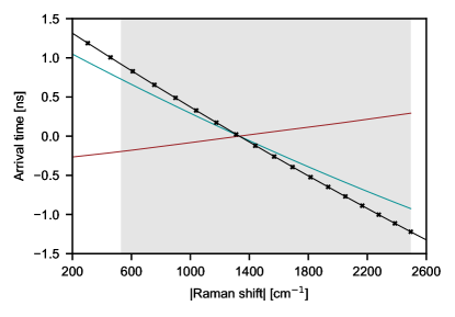
The arrival times of the Stokes and anti-Stokes photons are then calculated as
| (15) |
The time-to-digital converter is configured to receive the anti-Stokes signal as “start” input and the Stokes signal as “stop” input. Therefore, the coincidence time delay is defined by
| (16) |
Fig. 5 shows , and as a function of the absolute Raman shift with the time axis arbitrarily centered at the Raman resonance (). For simplicity, the calculated values of are fitted with the function , since the arrival time is inversely proportional to the group velocity and the refractive index can be expanded as . The measurements reported here and in the main text are calibrated by shifting the curves , and along the time axis to center the Raman peak at .
Diamond orientation.—
The tensor is a sum of electronic and Raman contributions with different weights depending on the field polarization relative to the crystal axes. When the pump polarization is aligned with the [001] axis of diamond, the Stokes and anti-Stokes photons generated through the exchange of a real phonon exhibit polarizations orthogonal to the pump. Consequently, the frequency difference between the Raman peak and the point of maximum destructive interference reaches its maximum value [35] (cf. Fig. 2). To realize this configuration, the diamond crystal is cut perpendicular to the [100] crystal axis and is mounted on a rotation stage. Since the pump polarization is fixed to vertical in the lab frame, the crystal is rotated to maximize the horizontally polarized Stokes power in order to align the [001] axis along the pump polarization (cf. Fig. 1).
Diamond anisotropy.— In a perfectly isotropic material the relationship between the electronic components of the susceptibility tensor should follow . With our definition of and in the main text this relationship translates into , ; we can thus define an anisotropy parameter
| (17) |
In diamond, it is expected that is small but non-zero because the electronic orbitals responsible for the third-order nonlinearity are not completely spherical. Moreover, the values of , and may change between different diamond samples depending on the presence of strain and defects, and they may depend on the excitation wavelength. In principle, the values of and can be extracted by coincidence measurements far from the Raman resonance, but the polarization response of the setup and the limited frequency range of our detection scheme affect the precision of this approach. Alternatively, the variation of the anisotropy parameters with wavelength can be deduced from the measurement of and
| (18) |
reported by Ref. [35] at various excitation wavelengths between and nm, and reproduced in Fig. 6 with full circles. The parameter represents the frequency difference between the Raman peak and the point of maximum destructive interference when the pump polarization is diagonal at and the polarizers in detection are parallel to the pump.
Fig. 6 shows that the value of we measure at nm (see main text) is in agreement with the measurements of Ref. [35]. Therefore, we can choose the parameters and to obtain a value of compatible with the same measurements. We select , since larger values lead to a drop in the parameter at low Raman shifts, where our measurements demonstrate . From Eq. 18, with compatible with Fig. 6 [35], we calculate an anisotropy factor of , and hence . These parameters are used for all the theoretical curves.
Bell test measurements.—
Fig. 7 clarifies the relationship between the Bell test and the two-photon interference measurements presented in the main text. The Bell test requires the measurements of the correlation parameter for the couples of detection angles , , , and where (cf. panel (a)). For each couple of angles, we perform coincidence measurements of hour with the Stokes and anti-Stokes polarizers set to , , , and . Then, the correlation parameter is computed from Eq. 11 and 13. Thereby, the CHSH parameters computed from Eq. 4 and shown in Fig. 3 are the result of coincidence measurements. The error bars are calculated by propagating the standard deviation of the coincidences in the region , where the counts are almost constant. To demonstrate two-photon interference, we perform additional measurements of for different polarization angles (cf. panel (b)). We notice that data points generally require coincidence measurements, although our choices of reduce this number to .