An Achievable Rate-Distortion Region of
Joint Identification and Sensing
for Multiple Access Channels

Abstract

In contrast to Shannon transmission codes, the size of identification (ID) codes for discrete memoryless channels (DMCs) experiences doubly exponential growth with the block length when randomized encoding is used. Additional enhancements within the ID paradigm can be realized through supplementary resources such as quantum entanglement, common randomness (CR), and feedback. Joint transmission and sensing demonstrate significant benefits over separation-based methods. Inspired by the significant impact of feedback on the ID capacity, our work delves into the realm of joint ID and sensing (JIDAS) for state-dependent multiple access channels (SD-MACs) with noiseless strictly casual feedback. Here, the senders aim to convey ID messages to the receiver while simultaneously sensing the channel states. We establish a lower bound on the capacity-distortion region of the SD-MACs. An example shows that JIDAS outperforms the separation-based approach.

I Introduction

Shannon’s groundbreaking work [1] laid the foundation for the transmission problem, revealing that the maximum number of reliably transmitted messages grows exponentially with block length. In today’s technological landscape including machine-to-machine systems [2], digital watermarking [3, 4, 5], industry 4.0 [6], and 6G communication systems [7, 8], the demand for improving data rates, latency, and security [7] is increasing. Many applications utilize Shannon’s transmission scheme, requiring receivers to decode all messages. However, this approach proves inefficient in various scenarios. Therefore, Ahlswede and Dueck [9], building on Jaja’s work [10], introduced the Identification (ID) scheme. Here, the receiver aims to decide whether a special message has been transmitted or not. Of course, the sender does not know which message is actually interesting to the receiver.

A groundbreaking result is demonstrated: when a randomized encoding scheme is employed, the size of identities experiences a doubly exponential growth with the block length. With only a deterministic coding scheme, despite scaling similarly to the transmission code, the ID rate still far surpasses the transmission rate for DMCs. Research demonstrates seamless integration of information-theoretic security into identification without added secrecy costs [11, 12]. Advancements in ID schemes can utilize resources such as quantum entanglement [13, 14], common randomness (CR) [15, 16, 17], and feedback [18]. Quantum entanglement is often more effective than CR. The study in [19] demonstrates that feedback does not increase transmission capacity for DMCs. However, feedback can increase ID capacity in noisy channels [18]. Identification in particular and post Shannon communication in general is a key approach to effectively implement important future applications to meet the cost and energy reduction challenges for future network operators [20].

In upcoming 6G networks, precise sensing of state information (SI) is vital for optimal performance [21, 22]. Traditionally, message transmission and sensing are handled separately, with resources divided for either estimating SI or communication through time-sharing. However, there is a trend towards merging them into a unified system and platform [23, 24]. Numerous recent studies have addressed the challenge of joint transmission and sensing [25, 26, 27, 28]. For example, the single-user DMCs have been explored in [29]. In their study, messages are transmitted, while an estimator on the sender’s side senses SI via causal feedback. They introduce a capacity-distortion trade-off, where the capacity is the supremum of achievable message transmission rates when ensuring that the distortion of sensing remains below a threshold value, representing the maximum distortion tolerable. Moreover, the work by [30] extended this model to MACs, and [31] addressed it within the context of broadcast channels (BC). In joint identification and sensing (JIDAS), using a noiseless feedback link benefits both the estimator and encoder. In [32], they study JIDAS with noiseless feedback over single-user DMCs, finding a lower bound of the deterministic ID capacity-distortion trade-off. The combination of Post Shannon communication and sensing can be expected to achieve additional synergies in the area of cost reduction and energy consumption reduction for future grid operators and users [20]. JDAS is the first example of this combination. Central research questions are still completely open [22].
The MAC models multiple senders communicating with a single receiver. A typical MAC scenario is the up-link of cellular systems, where multiple devices send data to a central base station. Initial characterization of the message transmission problem via a MAC was done by [33], with further details provided in [34]. The capacity of deterministic ID for MACs is explored in [35], while [36] investigates randomized ID capacity. Quantum entanglement’s enhancement of randomized ID via a MAC is shown in [37], with further advantages of perfect feedback discussed in [38]. To the best of our knowledge, the JIDAS problem for SD-MACs has not been addressed in the existing literature. In this work, we establish a lower bound on the ID capacity-distortion region for a two-sender state-dependent multiple access channel (K-SD-MAC) and demonstrate that our joint approach outperforms the separation-based scenario.
Outline: The remainder of the paper is structured as follows. In Section II, we introduce our system model and present the main results. In Section III, we establish proof of the lower bound on the ID capacity-distortion region for a K-SD-MAC. In Section IV, we provide an example to show the benefits of our joint approach. Section V concludes the paper.

II System Model and Main Results

Consider a K-Sender-SD-MAC (K-SD-MAC) $(\boldsymbol{\mathcal{X}}\times\boldsymbol{\mathcal{S}},W_{S}(y|\boldsymbol{x},\boldsymbol{s}),\mathcal{Y})$ with noiseless causal feedback as depicted in Fig. 1. The K-SD-MAC is described by a conditional probability distribution $W_{S}(Y|\boldsymbol{X},\boldsymbol{S})$. The channel input tuple $\boldsymbol{X}=\left(X_{1},\cdots,X_{K}\right)$, the channel state tuple $\boldsymbol{S}=\left(S_{1},\cdots,S_{K}\right)$, and the channel output $Y$ take values in finite sets $\boldsymbol{\mathcal{X}}=\mathcal{X}_{1}\times\cdots\times\mathcal{X}_{K}$, $\boldsymbol{\mathcal{S}}=\mathcal{S}_{1}\times\cdots\times\mathcal{S}_{K}$, and $\mathcal{Y}$, respectively. Given blocklength $n$, the state tuples $\boldsymbol{S}_{t}$ for all $t=1,\cdots,n$ are i.i.d. according to the joint distribution $P_{\boldsymbol{S}}$. We assume that the inputs $\boldsymbol{X}_{t}$, and the states $\boldsymbol{S}_{t}$ are statistically independent for all $t=1,\cdots,n$. The channel transition probability is memoryless, i.e., $W_{S}(y^{n}|\boldsymbol{x}^{n},\boldsymbol{s}^{n})=\prod_{t=1}^{n}{W(y_{t}|\boldsymbol{x}_{t},\boldsymbol{s}_{t})}$. The notation $D$ represents a one-symbol-time delay. The feedback is noiseless and strictly causal, that is, at time $t$ only $Y^{t-1}=[Y_{1},\cdots,Y_{t-1}]$ is available at encoders and estimators.

Figure 1: K-SD-MAC with noiseless causal feedback

We consider the following average channel:

$$W_{S\_avg}(y|\boldsymbol{x})=\sum_{\boldsymbol{s}\in\boldsymbol{\mathcal{S}}}P_{\boldsymbol{S}}(\boldsymbol{s})W_{S}(y|\boldsymbol{x},\boldsymbol{s}),$$

for all $\boldsymbol{x}\in\boldsymbol{\mathcal{X}}$, and $y\in\mathcal{Y}$.

Each encoder $k\in\mathcal{K}$ has a set of identities $\mathcal{N}_{k}=\left\{1,\cdots,N_{k}\right\}$. They independently send identities $i_{k}\in\mathcal{N}_{k}$ to the receiver. Each identity $i_{k}$ is encoded according to a strictly-causal noiseless feedback sequence $y^{t-1}$. The feedback encoding functions $\boldsymbol{f}_{k,i_{k}}$ is defined as follows.

Definition 1.

A feedback encoding function for identity $i_{k}\in\mathcal{N}_{k}$ is a vector-valued function

$$\boldsymbol{f}_{k,i_{k}}=\left[f_{k,i_{k}}^{1},\cdots,f_{k,i_{k}}^{n}\right],$$

where $f_{k,i_{k}}\in\mathcal{X}_{k}$, and for $t\in\left\{2,\cdots,n\right\}$, $f_{k,i_{k}}^{t}:\mathcal{Y}^{t-1}\mapsto\mathcal{X}_{k}$.

We denote the set of $\boldsymbol{f}_{k,i_{k}}$ with length $n$ as $\mathcal{F}_{k}^{n}$.

In the following, we define deterministic and randomized IDF codes for a K-SD-MAC.

Definition 2.

An $(n,\boldsymbol{N},\lambda)$ deterministic IDF code with $\lambda\in(0,\frac{1}{2})$ for K-SD-MAC $W_{S}$ is a system $\left\{(\boldsymbol{f}_{\boldsymbol{i}},\mathcal{D}_{\boldsymbol{i}})|\boldsymbol{i}\in\boldsymbol{\mathcal{N}}\right\}$, where

$$\boldsymbol{f}_{\boldsymbol{i}}\in\boldsymbol{\mathcal{F}}^{n},\quad\mathcal{D}_{\boldsymbol{i}}\subset\mathcal{Y}^{n}.$$

The probabilities of type I error and type II error for identity tuple $\boldsymbol{\mathcal{N}}$ satisfy

$$P_{e,1}\left(\boldsymbol{i}\right) \triangleq W_{S\_avg}\left(\mathcal{D}^{c}_{\boldsymbol{i}}|\boldsymbol{f}_{\boldsymbol{i}}\right)\leq\lambda,\quad\forall\boldsymbol{i}\in\boldsymbol{\mathcal{N}},$$

$$P_{e,2}\left(\boldsymbol{i},\tilde{\boldsymbol{i}}\right) \triangleq W_{S\_avg}(\mathcal{D}_{\boldsymbol{\tilde{i}}}|\boldsymbol{f}_{\boldsymbol{i}})\leq\lambda,\quad\forall\boldsymbol{i},\tilde{\boldsymbol{i}}\in\boldsymbol{\mathcal{N}},\tilde{\boldsymbol{i}}\neq\boldsymbol{i}.$$

Definition 3.

    An $(n,\boldsymbol{N},\lambda)$ randomized IDF code with $\lambda\in(0,\frac{1}{2})$ for K-SD-MAC $W_{S}$ is a system $\left\{(Q(\cdot|\boldsymbol{i}),\mathcal{D}_{\boldsymbol{i}})|\boldsymbol{i}\in\boldsymbol{\mathcal{N}}\right\}$ with

$$Q(\cdot|\boldsymbol{i})\in\mathcal{P}(\boldsymbol{\mathcal{F}}^{n}),\quad\mathcal{D}_{\boldsymbol{i}}\subset\mathcal{Y}^{n},$$

where $Q(\cdot|\boldsymbol{i})=\prod_{k=1}^{K}Q_{k}(\cdot|i_{k})$, and $Q_{k}(\cdot|i_{k})\in\mathcal{P}(\mathcal{F}_{k}^{n})$.

The probabilities of type I error and type II error for identity tuple $\boldsymbol{\mathcal{N}}$ satisfy

$$P_{e,1}\left(\boldsymbol{i}\right) \triangleq\sum_{\boldsymbol{f}\in\boldsymbol{\mathcal{F}}^{n}}Q(\boldsymbol{f}|i)W_{S\_avg}^{n}(\mathcal{D}_{\boldsymbol{i}}^{c}|\boldsymbol{f})\leq\lambda,\quad\forall\boldsymbol{i}\in\boldsymbol{\mathcal{N}},$$

$$P_{e,2}\left(\boldsymbol{i},\tilde{\boldsymbol{i}}\right) \triangleq\sum_{\boldsymbol{f}\in\boldsymbol{\mathcal{F}}^{n}}Q(\boldsymbol{f}|i)W_{S\_avg}^{n}(\mathcal{D}_{\boldsymbol{\tilde{i}}}^{c}|\boldsymbol{f})\leq\lambda,$$

$$\forall\boldsymbol{i},\boldsymbol{\tilde{i}}\in\boldsymbol{\mathcal{N}} ,\boldsymbol{i}\neq\boldsymbol{\tilde{i}}.$$

Simultaneously, estimator $k$ senses its respective states $S_{k}$, generating estimation $\hat{S}_{k,t-1}$ with respect to feedback symbol $Y_{t-1}$ and input symbol $X_{k,t-1}$. The performance of estimators is evaluated based on the expected distortion over $(S_{k},\hat{S_{k}})$, i.e.,

$$\mathbb{E}\left[d(S_{k}^{n},\hat{S}_{k}^{n})\right]=\frac{1}{n}\sum_{t=1}^{n}{\mathbb{E}\left[d(S_{k,t},\hat{S}_{k,t})\right]},$$ (1)

where $d(\cdot,\cdot):\hat{\mathcal{S}}_{k}\times\mathcal{S}_{k}\mapsto\mathbb{R}$ is a general distortion function, e.g., Hamming distance, or mean square error (MSE).

We define the estimation functions $h_{k}:\mathcal{X}_{k}\times\mathcal{Y}\mapsto\mathcal{S}_{k}$, and denote the sets of all $h_{k}$ as $\mathcal{H}_{k}$. Without loss of generality, deterministic estimators $h^{*}_{k}(\cdot,\cdot)$ can be employed, defined as follows:

$$h^{*}_{k}(x_{k},y)=\underset{{h_{k}\in\mathcal{H}_{k}}}{\arg\min}\mathbb{E}_{S_{k}}\left[d(S_{k},h(X_{k},Y))|X_{k}=x_{k},Y=y\right].$$

We define the minimal distortion for each input symbol and input distribution, respectively, achieved by the deterministic estimator described above.

Definition 4.

For each input-symbol $x_{k}\in\mathcal{X}_{k}$, the minimal distortion $d_{k}^{*}(x_{k})$ is given by

$$d_{k}^{*}(x_{k})=\mathbb{E}_{S_{k}Y}\left[d(S_{k},h_{k}^{*}(X_{k},Y))|X_{k}=x_{k}\right].$$

Similarly, for each input distribution $P_{k}\in\mathcal{P}(\mathcal{X}_{k})$, the minimal distortion $d_{k}^{*}(P_{k})$ is given by

$$d_{k}^{*}(P_{k})=\sum_{x_{k}\in\mathcal{X}_{k}}P_{k}(x_{k})d_{k}^{*}(x_{k}).$$

Thus, for the deterministic coding strategies $\boldsymbol{f}_{i}$ and $\boldsymbol{g}_{j}$, we can express the expected distortions (1) as follows:

$$\bar{d}^{n}_{k} =\frac{1}{N_{k}}\sum_{i_{k}=1}^{N_{k}}\frac{1}{n}\sum_{t=1}^{n}d_{k}^{*}(f_{k,i_{k}}^{t}).$$

Similarly, for randomized coding strategy $Q(\cdot|\boldsymbol{i})$, we can represent the average distortion as follows:

$$\bar{d}_{k}^{n}=\frac{1}{N_{k}}\sum_{i_{k}=1}^{N_{k}}\sum_{\boldsymbol{f}_{k}\in\mathcal{F}_{k}^{n}}Q_{k}(\boldsymbol{f}_{k}|i_{k})\frac{1}{n}\sum_{t=1}^{n}d_{k}^{*}\left(f_{k,i_{k}}^{t}\right).$$

Definition 5.

1. A rate-distortion tuple $\boldsymbol{R}(\boldsymbol{D})\triangleq(R_{1}(\boldsymbol{D}),\cdots,R_{K}(\boldsymbol{D}))$ with vector-valued constant $\boldsymbol{D}=\left(D_{1},\cdots,D_{K}\right)$ representing the maximum tolerated distortions is said to be achievable, if there exists an $(n,\boldsymbol{\mathcal{N}},\lambda)$ IDF code for K-SD-MAC $W_{S}$, such that for all $k\in\mathcal{K}$, $\limsup_{n\to\infty}\bar{d}^{n}_{k}\leq D_{k}$.

2. The ID capacity-distortion region $\mathcal{C}(\boldsymbol{D})=\left\{R_{1}(\boldsymbol{D}),\cdots,R_{K}(\boldsymbol{D})\right\}$ is defined as the closure of all achievable rate-distortion tuples.

Theorem 6.

If all senders can transmit with positive rates, then the deterministic ID capacity-distortion region $\mathcal{C}_{ID}^{d}(\boldsymbol{D})$ of a K-SD-MAC $W_{S}$ is lower-bounded by

$$\begin{split}\mathcal{C}_{ID}^{d}(\boldsymbol{D})=\Biggl{\{}\boldsymbol{R}(\boldsymbol{D}):R_{k}(\boldsymbol{D})\geq&\max_{\boldsymbol{x}\in\boldsymbol{\mathcal{X}}^{D}}H(W_{S\_avg}(\cdot|\boldsymbol{x}))\Biggr{\}},\end{split}$$ (2)

where $\boldsymbol{\mathcal{X}}^{D}=\mathcal{X}_{1}^{D_{1}}\times\cdots\times\mathcal{X}_{K}^{D_{K}}$, and $\mathcal{X}_{k}^{D_{k}}=\left\{x_{k}\in\mathcal{X}_{k}|d_{k}^{*}(x_{k})\leq D_{k}\right\}$ representing the sets of admissible input symbols.

Theorem 7.

If all senders can transmit with positive rates, then the randomized ID capacity-distortion region $\mathcal{C}_{ID}^{r}(\boldsymbol{D})$ of a K-SD-MAC $W_{S}$ is lower-bounded by

$$\begin{split}\mathcal{C}_{ID}^{r}(\boldsymbol{D})=\Biggl{\{}\boldsymbol{R}(\boldsymbol{D}):R_{k}(\boldsymbol{D})\geq&\max_{\boldsymbol{P}\in\boldsymbol{\mathcal{P}}^{\boldsymbol{D}}}H\left(\boldsymbol{P}W_{S\_avg}\right)\Biggr{\}},\end{split}$$ (3)

where $\boldsymbol{\mathcal{P}}^{\boldsymbol{D}}=\mathcal{P}_{1}^{D_{1}}\times\cdots\times\mathcal{P}_{K}^{D_{K}}$, and $\mathcal{P}_{k}^{D_{k}}=\left\{P_{k}\in\mathcal{P}(\mathcal{X}_{k})|d_{k}^{*}(P_{k})\leq D_{k}\right\}$ denoting the set of admissible input distributions. $W_{S\_avg}(y)=\sum_{\boldsymbol{x}\in\boldsymbol{\mathcal{X}}}\boldsymbol{P}(\boldsymbol{x})W_{S\_avg}(y|\boldsymbol{x})$, for all $y\in\mathcal{Y}$ is a distribution over $\mathcal{Y}$.

Remark 8.

As long as all senders can transmit with positive rates, there is no trade-off between two senders. Moreover, the weaker sender (with lower transmission capacity) can achieve the same rate as the stronger sender.

Remark 9.

As long as all senders can transmit with positive rates, there is no trade-off between two senders. Moreover, the weaker sender (with lower transmission capacity) can achieve the same rate as the stronger sender.

III Proof

In this section, we provide the proofs of Theorem 6 and Theorem 7. It suffices to show that the above-mentioned rate-distortion regions are achievable for the average channel $W_{S\_avg}$.

III-A Proof of Theorem 6

We extend the encoding scheme for IDF through single-user channels, as outlined in [18], to our JIDAS problem via a K-SD-MAC. Consider an $(m,\boldsymbol{\mathcal{N}},\lambda)$ deterministic IDF code, where $m=n+\lceil\sqrt{n}\rceil$. The encoders use first $n$ bits to generate common randomness by sending $\boldsymbol{x}^{*n}$, where

$$\boldsymbol{x}^{*}=\underset{\boldsymbol{x}\in\boldsymbol{\mathcal{X}}^{\boldsymbol{D}}}{\arg\max}H(W_{S\_avg}(\cdot|\boldsymbol{x})).$$ (4)

The sequences $y^{n}$ sharing among encoders, estimators (via noiseless feedback links) and decoder (via channel) can be regarded as outcomes of random experiments $\left(\mathcal{Y}^{n},W_{S\_avg}^{n}(Y^{n}|\boldsymbol{x}^{*n})\right)$. However, it is not uniformly distributed across the sample space, presenting challenges in constructing codes. The theorem about typical sequences provides solutions to address this concern. We denote $\mathcal{D}^{*}=\mathcal{T}_{\epsilon}^{n}(W_{S\_avg}(\cdot|\boldsymbol{x}^{*}))$ as the set of typical sequences and $e=\mathcal{Y}/\mathcal{D}^{*}$ as the set of errors. By choosing small $\epsilon$ and sufficient large $n$, we have the following lemma:

Lemma 10.

Suppose $y^{n}\in\mathcal{D}^{*}$, and $Y^{n}$ is emitted by $W_{S\_avg}(\cdot|\boldsymbol{x}^{*})$, then

$$W_{S\_avg}^{n}(y^{n}|\boldsymbol{x}^{*n}) \doteq 2^{-nH(W(\cdot|\boldsymbol{x}^{*}))},$$

$$|\mathcal{D}^{*}| \doteq 2^{nH(W(\cdot|\boldsymbol{x}^{*}))},$$

$$W_{S\_avg}^{n}(\mathcal{D}^{*}|\boldsymbol{x}^{*n}) \doteq 1,$$

where $\doteq$ denotes the asymptotic equivalence in $n$.

Thus, without loss generality, we convert the random experiment to a uniform one $\left(\mathcal{D}^{*},W_{S\_avg}(y|\boldsymbol{x})\right)$.

Next, we introduce families of ”coloring functions”, denoted as $\left\{F_{k,i_{k}}|i_{k}=1,\cdots,N_{k}\right\}$ for all $k\in\mathcal{K}$. Each function $F_{k,i_{k}}:\quad\mathcal{D}^{*}\mapsto\mathcal{M}_{k}=\left\{1,\cdots,M_{k}\right\}$ maps the sequence $y^{n}\in\mathcal{D}^{*}$ to a ”color” $l_{k}\in\mathcal{M}_{k}$. We denote the tuple of ”coloring functions” as $\boldsymbol{F}_{\boldsymbol{i}}=\left(F_{1,i_{1}},\cdots,F_{K,i_{K}}\right)$, the tuple of ”colors” as $\boldsymbol{l}=\left(l_{1},\cdots,l_{K}\right)$, the tuple of the color sets as $\boldsymbol{\mathcal{M}}=\left(\mathcal{M}_{1},\cdots,\mathcal{M}_{K}\right)$, and their cardinality as $\boldsymbol{M}=\left(M_{1},\cdots,M_{K}\right)$. We uniformly and randomly generate the functions, i.e., $Pr\left[F_{k,i_{k}}(y^{n})=l_{k}\right]=\frac{1}{M_{k}}$. The mappings $F_{k,i_{k}}$ serve as prior knowledge for all encoders and the decoder.

After receiving $y^{n}\in\mathcal{D}^{*}$ via feedback, the encoders calculate and transmit $F_{k,i_{k}}(y^{n})$, using a ”normal” $\left(\lceil\sqrt{n}\rceil,\boldsymbol{M},2^{-\lceil\sqrt{n}\rceil\delta}\right)$ transmission code denoted as $\mathcal{C}^{\prime}=\left\{\left(\boldsymbol{c}(\boldsymbol{l}),\mathcal{D}^{\prime}_{\boldsymbol{l}}\right)\big{|}\boldsymbol{l}\in\mathcal{M}\right\}$. In the following process of analysis, we use $\boldsymbol{c}=\left(\boldsymbol{c}_{1},\cdots,\boldsymbol{c}_{K}\right)$ to denote $\boldsymbol{c}\left(\boldsymbol{F}_{\boldsymbol{i}}(y^{n})\right)$. Notably, we need to choose the code words under distortion constraints, i.e., $\bar{d}_{k}(\boldsymbol{c})=\frac{1}{\lceil\sqrt{n}\rceil}\sum_{t=1}^{\lceil\sqrt{n}\rceil}d_{k}^{*}(c_{k,t})\leq D_{k}$ for all $k\in\mathcal{K}$. If $y^{n}\in e$, an error is declared. But according to Lemma 10, this error occurs with a probability close to $0$. The decoder first computes $F_{i^{\prime}_{k}}(y^{n})$. Then, it decodes $\hat{{F}_{i_{k}}}$ based on $y_{n+1}^{m}$. If ${F}_{i^{\prime}_{k}}(y^{n})=\hat{F}_{i_{k}}$, it concludes $i_{k}=i^{\prime}_{k}$; otherwise, $i_{k}\neq i^{\prime}_{k}$.

In conclusion, for feedback sequences $y^{n}\in\mathcal{D}^{*}$, our deterministic IDF code is defined as

$$\boldsymbol{f}_{k,i_{k}} =\left[x_{k}^{*n},\boldsymbol{c}_{k}\right],\quad x_{k}^{*}\in\mathcal{X}_{k}^{D_{k}},\quad\bar{d}_{k}(\boldsymbol{c}_{k})\leq D_{k},\quad\forall k\in\mathcal{K},$$

$$\mathcal{D}_{\boldsymbol{i}} =\bigcup_{y^{n}\in\mathcal{D}^{*}}y^{n}\times\mathcal{D}^{\prime}_{\boldsymbol{F}_{\boldsymbol{i}}(y^{n})},\quad\forall\boldsymbol{i}\in\boldsymbol{\mathcal{N}},$$

where $\boldsymbol{x}_{k}$ follows (4).

For all $\boldsymbol{i}\in\boldsymbol{\mathcal{N}}$, the type I error probability at Sender k $P_{e,1}(\boldsymbol{i})$ can be upper-bounded by:

$$W_{S\_avg}^{m}(\mathcal{D}_{\boldsymbol{i}}^{c}|\boldsymbol{f}_{\boldsymbol{i}})$$

$$=\sum_{y^{n}\in\mathcal{D}^{*}}W_{S\_avg}^{n}\left(y^{n}|\boldsymbol{x}^{*n}\right)\cdot W_{S\_avg}^{\lceil\sqrt{n}\rceil}\left(D^{\prime c}_{\boldsymbol{F}_{\boldsymbol{i}}}(y^{n})|\boldsymbol{c}\right)$$

$$\leq 2^{-\lceil\sqrt{n}\rceil\delta}=\circ(n).$$

Thus, we can achieve an arbitrary small type I error probability with sufficient large code length.

Without the loss of generality, we examine the type II error probability $P^{1}_{e,2}$ for the identity set $\mathcal{N}_{1}$. We first introduce the definition of the following sets for all $\boldsymbol{i},\boldsymbol{i}^{\prime}\in\boldsymbol{\mathcal{N}}$.

$$F_{i_{1}}\cap F_{i^{\prime}_{1}} :=\left\{y\in\mathcal{D}^{*}|F_{1,i_{1}}(y^{n})=F_{1,i^{\prime}_{1}}(y^{n})\right\},$$

$$F_{i/i_{1}}\cap F_{i^{\prime}/i^{\prime}_{1}} :=\left\{y\in\mathbb{R}|\boldsymbol{F}_{\boldsymbol{i/i_{1}}}(y^{n})=\boldsymbol{F}_{\boldsymbol{i^{\prime}/i^{\prime}_{1}}}(y^{n})\right\},$$

$$F_{i_{1}}-F_{i^{\prime}_{1}} :=\left\{y\in\mathcal{D}^{*}|F_{1,i_{1}}(y^{n})\neq F_{1,i^{\prime}_{1}}(y^{n})\right\},$$

$$F_{i/i_{1}}-F_{i^{\prime}/i^{\prime}_{1}} :=\left\{y\in\mathcal{D}^{*}|\boldsymbol{F}_{\boldsymbol{i/i_{1}}}(y^{n})\neq\boldsymbol{F}_{\boldsymbol{i^{\prime}/i^{\prime}_{1}}}(y^{n})\right\},$$

where $\boldsymbol{i/i_{1}}=(i_{2},\cdots,i_{K})$ and $\boldsymbol{i^{\prime}/i^{\prime}_{1}}=(i^{\prime}_{2},\cdots,i^{\prime}_{K})$.

Then, for all $\boldsymbol{i},\boldsymbol{\tilde{i}}\in\boldsymbol{\mathcal{N}}$, $\boldsymbol{i}\neq\boldsymbol{\tilde{i}}$, the type II error probability $P_{e2}^{1}(\boldsymbol{i},\boldsymbol{\tilde{i}})$ at Sender 1 can be upper-bounded by:

$$W_{S\_avg}^{m}(\mathcal{D}_{\boldsymbol{\tilde{i}_{1}}}|\boldsymbol{f}_{\boldsymbol{i}})$$

$$\leq\sum_{y^{n}\in\{F_{i_{1}}\cap F_{\tilde{i}_{1}}\}\cap\{F_{i/i_{1}}\cap F_{i^{\prime}/i^{\prime}_{1}}\}}W_{S\_avg}^{n}(y^{n}|\boldsymbol{x}^{*n})$$

$$\quad+\sum_{y^{n}\in\{F_{i_{1}}-F_{\tilde{i}_{1}}\}\cup\{F_{i/i_{1}}-F_{i^{\prime}/i^{\prime}_{1}}\}}W_{S\_avg}^{n}(y^{n}|\boldsymbol{x}^{*n})\cdot 2^{-\lceil\sqrt{n}\rceil\delta}$$

$$\leq\frac{|F_{i_{1}}\cap F_{\tilde{i}_{1}}|}{|\mathcal{D}^{*}|}+\circ(n).$$

Define an auxiliary random variable $\Psi_{y^{n}}$ for all $y^{n}\in\mathcal{D}^{*}$, where

$$\Psi_{y^{n}}(F_{\tilde{i}})=\left\{\begin{array}[]{cc}1,&y^{n}\in F_{i_{1}}\cap F_{\tilde{i}_{1}}\\ 0,&y^{n}\in F_{i_{1}}-F_{\tilde{i}_{1}}\end{array},\right.$$

with probability $Pr[\Psi_{y^{n}}(F_{\tilde{i}})=1]=\frac{1}{M_{1}}$.

Lemma 11.

[18] For $\lambda\in(0,1)$, and $E[\Psi_{y^{n}}]=\frac{1}{M_{1}}<\lambda$,

$$Pr\left[\frac{1}{|\mathcal{D}^{*}|}\sum_{y^{n}\in\mathcal{D}^{*}}\Psi_{y^{n}}(F_{2})>\lambda\right]<2^{-|\mathcal{D}^{*}|\cdot(\lambda\log(M_{1})-1)}.$$

For all pairs $(i_{1},\tilde{i}_{1})\in\mathcal{N}_{1}^{2}$, $i_{1}\neq\tilde{i}_{1}$, we need to upper-bound $\frac{|F_{i_{1}}\cap F_{\tilde{i}_{1}}|}{|\mathcal{D}^{*}|}$ by $\lambda$. Thus, the following probability

$$Pr\left[\bigcap_{\tilde{i}\in\mathcal{N}_{1},\tilde{i}\neq i}\left\{\frac{1}{|\mathcal{D}^{*}|}\sum_{y^{n}\in\mathcal{D}^{*}}\Psi_{y^{n}}(F_{\tilde{i}})\leq\lambda\right\}\right]$$

$$\quad\geq 1-(N_{1}-1)\cdot 2^{-2^{nH(W_{S\_avg}(\cdot|\boldsymbol{x}^{*})}\cdot(\lambda\log{M_{1}}-1)}$$

should be greater than $0$. Therefore, the maximum value of $N_{1}$ we can choose is:

$$N_{1}=2^{2^{nH(W_{S\_avg}(\cdot|\boldsymbol{x}^{*}))}\cdot(\lambda\log{M_{1}}-1)}.$$

This implies that as $m$ goes to infinity, the rate at Sender 1 can achieve:

$$\lim_{m\to\infty}R_{1}(\boldsymbol{D}) =\lim_{m\to\infty}\frac{\log\log{N_{1}}}{m}=H(W_{S\_avg}(\cdot|\boldsymbol{x}^{*})).$$

Similarly, if the rate at any Sender $k\in\mathcal{K}$ takes the value

$$\lim_{m\to\infty}R_{k}(\boldsymbol{D})=H(W_{S\_avg}(\cdot|\boldsymbol{x}^{*})),$$

then the type II error probability at Sender $k$ can also be upper-bounded by $\lambda$. Regarding distortion, our coding scheme guarantees:

$$\bar{d}_{k}^{m} =\frac{1}{N_{k}}\sum_{i_{k}=1}^{N_{k}}\frac{1}{m}\left(n\cdot d_{k}^{*}(x_{k}^{*})+\lceil\sqrt{n}\rceil\cdot\bar{d}(\boldsymbol{c}_{k}\left(F_{i}(y^{n}\right)))\right)\leq D_{k},$$

This completes the proof of Theorem 6.

III-B Sketch of Proof of Theorem 7

Similarly, consider a randomized IDF code with code length $m=n+\lceil\sqrt{n}\rceil$. The first $n$ bits are generated according to the same probability distribution $\boldsymbol{P}^{*}$, where

$$\boldsymbol{P}^{*}=\underset{{\boldsymbol{P}\in\mathcal{P}(\boldsymbol{\mathcal{X}})}}{\arg\max}H(\boldsymbol{P}W_{S\_avg}).$$

We convert it to an uniformly distributed random experiment $\left(\mathcal{D}^{*},\boldsymbol{P}^{*}W_{S\_avg}\right)$, where $\mathcal{D}^{*}=\mathcal{T}_{\epsilon}^{n}(\boldsymbol{P}^{*}W_{S\_avg})$. The consequent encoding steps are similar to the deterministic case.
In conclusion, our randomized IDF code can be represented as follows:

$$Q_{F}(\boldsymbol{f}_{k}|i_{k}) ={\boldsymbol{P}_{k}^{*}}^{n}\times\mathbbm{1}\left(\boldsymbol{f}_{k,n+1}^{m}=c_{k}\right),$$

$$P_{k}^{*} \in\mathcal{P}_{k}^{D_{k}},\bar{d}_{k}(\boldsymbol{c}_{k})\leq D_{k},\quad\forall k\in\mathcal{K},$$

$$\mathcal{D}_{\boldsymbol{i}} =\bigcup_{y^{n}\in\mathcal{D}^{*}}y^{n}\times\mathcal{D}^{\prime}_{\boldsymbol{F}_{\boldsymbol{i}}(y^{n})},\quad\forall\boldsymbol{i}\in\boldsymbol{\mathcal{N}}.$$

Similarly, we can achieve an arbitrary small type I error probability with sufficient large code length. With

$$\lim_{m\to\infty}R_{k}(\boldsymbol{D})=\max_{\boldsymbol{P}\in\boldsymbol{\mathcal{P}}^{\boldsymbol{D}}}H(\boldsymbol{P}W_{S\_avg})$$

we can upper-bound the probabilities of type II error at any Sender $K$ by $\lambda$.
The distortion constraints are satisfied as follows:

$$\bar{d}_{k}^{m} =\frac{1}{N_{k}}\sum_{i_{k}=1}^{N_{k}}\frac{1}{m}\left(n\cdot d_{k}^{*}(P_{k}^{*})+\lceil\sqrt{n}\rceil\cdot\bar{d}_{k}(\boldsymbol{c}_{k}(\boldsymbol{F}_{\boldsymbol{i}}(y^{n})))\right)\leq D_{k}.$$

This completes the proof of Theorem 7.

IV Example

Consider a binary adder 2-SD-MAC with distributed multiplicative Bernoulli states, where $Y=X_{1}\cdot S_{1}\oplus X_{2}\cdot S_{2}$. We assume $\mathcal{X}_{1}=\mathcal{X}_{2}=\mathcal{S}_{1}=\mathcal{S}_{2}=\mathcal{Y}=\{0,1\}$, and $S_{1},S_{2}\sim Ber(p_{S})$ are i.i.d. for all $t=1,\cdots,n$. Hamming distance is used as the distortion function, i.e., $d(S_{k},\hat{S}_{k})=S_{k}\oplus\hat{S}_{k}$. The estimates are given by

$$\hat{s}_{k}=h_{k}^{*}(x_{k},y)=\underset{s^{\prime}_{k}\in\{0,1\}}{\arg\max}P_{S_{k}|X_{k}Y}(s^{\prime}_{k}|x_{k},y).$$

For deterministic ID, the minimal distortions of $x_{k}$ are given by

$$d_{k}^{*}(x_{k}) =\sum_{y}P_{Y|X_{k}}(y|x_{k})\min_{s^{\prime\prime}_{k}\in\{0,1\}}P_{S_{k}|X_{k}Y}(s^{\prime\prime}_{k}|x_{k},y).$$

The extreme points are listed in TABLE I.

$x_{1}$	$x_{2}$	$Y$	$d_{1}^{*}(x_{1})$	$d_{2}^{*}(x_{2})$	$R_{1},R_{2}\geq$
$0$	$1$	$S_{2}$	$\min\{p_{S},1-p_{S}\}$	$0=D_{2,min}$	$H_{2}(p_{S})$
$1$	$0$	$S_{1}$	$0=D_{1,min}$	$\min\{p_{S},1-p_{S}\}$	$H_{2}(p_{S})$
$1$	$1$	$S_{1}\oplus S_{2}$	$p_{S}=D_{1,max}$	$p_{S}=D_{2,max}$	$H_{2}\left(2p_{S}(1-p_{S})\right)=R_{max}$

TABLE I: Extreme points of lower-bound of deterministic ID capacity-distortion region

For randomized ID, we assume $X_{1}\sim Ber(p_{1})$ and $X_{2}\sim Ber(p_{2})$. The minimal distortions of $P_{k}$ are given by

$$d_{k}^{*}(p_{k})=(1-p_{k})d^{*}(0)+p_{k}d^{*}(1).$$

Our lower bounds of the randomized ID capacity-distortion region are illustrated in Fig. 2. It is evident that our joint approach results in a significant enhancement compared to the separation-based method achieved by splitting the resources either estimating the SI or communication, especially when $p_{S}\approx\frac{1}{2}$. Note that not every pair $(D_{1},D_{2})$ is achievable.

(a) Lower bound of $\mathcal{C}^{r}_{ID}(\boldsymbol{D})$with $p_{S}=0.2$

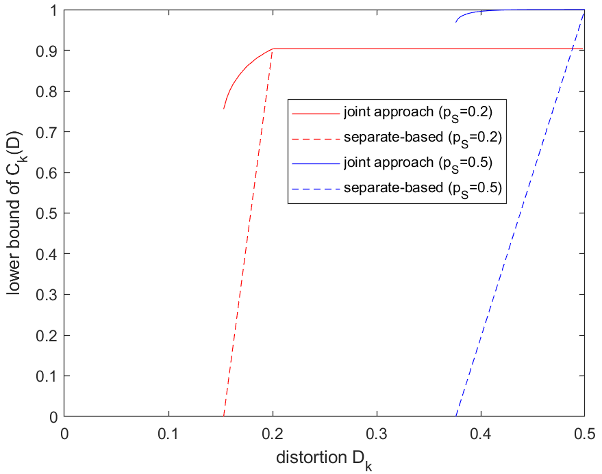
(b) Lower bound of $C^{r}_{k}(\boldsymbol{D})$ with assumption $D_{1}=D_{2}$

Figure 2: Joint approach vs. separation-based approach

V Conclusions

In our work, we studied the problem of joint ID and channel state sensing over a 2-SD-MAC where two i.i.d. channel states are generated jointly. Each sender is equipped with an estimator tasked with sensing the respective channel state based on input and feedback. Our contribution lies in establishing lower bounds for both deterministic and randomized ID capacity-distortion regions in this setup. Future research directions could focus on establishing the converse proof of the JIDAS problem. Additionally, extending this problem to Gaussian channels would also be interesting.

References

• [1] C. E. Shannon, “A mathematical theory of communication,” The Bell system technical journal, vol. 27, no. 3, pp. 379–423, 1948.
• [2] H. Boche and C. Deppe, “Secure identification for wiretap channels; robustness, super-additivity and continuity,” IEEE Transactions on Information Forensics and Security, vol. 13, no. 7, pp. 1641–1655, 2018.
• [3] P. Moulin, “The role of information theory in watermarking and its application to image watermarking,” Signal Processing, vol. 81, no. 6, pp. 1121–1139, 2001.
• [4] R. Ahlswede and N. Cai, “Watermarking identification codes with related topics on common randomness,” General Theory of Information Transfer and Combinatorics, pp. 107–153, 2006.
• [5] Y. Steinberg and N. Merhav, “Identification in the presence of side information with application to watermarking,” IEEE Transactions on Information Theory, vol. 47, no. 4, pp. 1410–1422, 2001.
• [6] Y. Lu, “Industry 4.0: A survey on technologies, applications and open research issues,” Journal of industrial information integration, vol. 6, pp. 1–10, 2017.
• [7] G. P. Fettweis and H. Boche, “On 6G and trustworthiness,” Communications of the ACM, vol. 65, no. 4, pp. 48–49, 2022.
• [8] J. A. Cabrera, H. Boche, C. Deppe, R. F. Schaefer, C. Scheunert, and F. H. Fitzek, “6G and the post-Shannon theory,” Shaping Future 6G Networks: Needs, Impacts, and Technologies, pp. 271–294, 2021.
• [9] R. Ahlswede and G. Dueck, “Identification via channels,” IEEE Transactions on Information Theory, vol. 35, no. 1, pp. 15–29, 1989.
• [10] J. J. Ja, “Identification is easier than decoding,” in 26th Annual Symposium on Foundations of Computer Science (sfcs 1985).   IEEE, 1985, pp. 43–50.
• [11] R. Ahlswede and Z. Zhang, “New directions in the theory of identification via channels,” IEEE transactions on information theory, vol. 41, no. 4, pp. 1040–1050, 1995.
• [12] W. Labidi, C. Deppe, and H. Boche, “Secure identification for Gaussian channels,” in ICASSP 2020-2020 IEEE International Conference on Acoustics, Speech and Signal Processing (ICASSP).   IEEE, 2020, pp. 2872–2876.
• [13] H. Boche, C. Deppe, and A. Winter, “Secure and robust identification via classical-quantum channels,” IEEE Transactions on Information Theory, vol. 65, no. 10, pp. 6734–6749, 2019.
• [14] U. Pereg, J. Rosenberger, and C. Deppe, “Identification over quantum broadcast channels,” in 2022 IEEE International Symposium on Information Theory (ISIT).   IEEE, 2022, pp. 258–263.
• [15] R. Ezzine, M. Wiese, C. Deppe, and H. Boche, “Common randomness generation from finite compound sources,” arXiv preprint arXiv:2401.14323, 2024.
• [16] ——, “Common randomness generation over slow fading channels,” in 2021 IEEE International Symposium on Information Theory (ISIT).   IEEE, 2021, pp. 1925–1930.
• [17] W. Labidi, R. Ezzine, C. Deppe, and H. Boche, “Common randomness generation from gaussian sources,” arXiv preprint arXiv:2201.11078, 2022.
• [18] R. Ahlswede and G. Dueck, “Identification in the presence of feedback-a discovery of new capacity formulas,” IEEE Transactions on Information Theory, vol. 35, no. 1, pp. 30–36, 1989.
• [19] J. Wolfowitz, Coding theorems of information theory.   Springer Science & Business Media, 2012, vol. 31.
• [20] P. Schwenteck, G. T. Nguyen, H. Boche, W. Kellerer, and F. H. P. Fitzek, “6g perspective of mobile network operators, manufacturers, and verticals,” IEEE Network Letters, vol. 5, no. 3, pp. 169–172, 2023.
• [21] A. Bourdoux, A. N. Barreto, B. van Liempd, C. de Lima, D. Dardari, D. Belot, E.-S. Lohan, G. Seco-Granados, H. Sarieddeen, H. Wymeersch et al., “6G white paper on localization and sensing,” arXiv preprint arXiv:2006.01779, 2020.
• [22] G. P. Fettweis and H. Boche, “6g: The personal tactile internet—and open questions for information theory,” IEEE BITS the Information Theory Magazine, vol. 1, no. 1, pp. 71–82, 2021.
• [23] L. Zheng, M. Lops, Y. C. Eldar, and X. Wang, “Radar and communication coexistence: An overview: A review of recent methods,” IEEE Signal Processing Magazine, vol. 36, no. 5, pp. 85–99, 2019.
• [24] F. Liu, C. Masouros, A. P. Petropulu, H. Griffiths, and L. Hanzo, “Joint radar and communication design: Applications, state-of-the-art, and the road ahead,” IEEE Transactions on Communications, vol. 68, no. 6, pp. 3834–3862, 2020.
• [25] C. Sturm and W. Wiesbeck, “Waveform design and signal processing aspects for fusion of wireless communications and radar sensing,” Proceedings of the IEEE, vol. 99, no. 7, pp. 1236–1259, 2011.
• [26] D. W. Bliss, “Cooperative radar and communications signaling: The estimation and information theory odd couple,” in 2014 IEEE Radar Conference.   IEEE, 2014, pp. 0050–0055.
• [27] M. Bica, K.-W. Huang, U. Mitra, and V. Koivunen, “Opportunistic radar waveform design in joint radar and cellular communication systems,” in 2015 IEEE Global Communications Conference (GLOBECOM).   IEEE, 2015, pp. 1–7.
• [28] K.-W. Huang, M. Bică, U. Mitra, and V. Koivunen, “Radar waveform design in spectrum sharing environment: Coexistence and cognition,” in 2015 IEEE Radar Conference (RadarCon).   IEEE, 2015, pp. 1698–1703.
• [29] M. Kobayashi, G. Caire, and G. Kramer, “Joint state sensing and communication: Optimal tradeoff for a memoryless case,” in 2018 IEEE International Symposium on Information Theory (ISIT).   IEEE, 2018, pp. 111–115.
• [30] M. Ahmadipour, M. Wigger, and M. Kobayashi, “Coding for sensing: An improved scheme for integrated sensing and communication over macs,” in 2022 IEEE International Symposium on Information Theory (ISIT), 2022, pp. 3025–3030.
• [31] M. Ahmadipour and M. Wigger, “An information-theoretic approach to collaborative integrated sensing and communication for two-transmitter systems,” IEEE Journal on Selected Areas in Information Theory, vol. 4, pp. 112–127, 2023.
• [32] W. Labidi, C. Deppe, and H. Boche, “Joint identification and sensing for discrete memoryless channels,” in 2023 IEEE International Symposium on Information Theory (ISIT).   IEEE, 2023, pp. 442–447.
• [33] H. H.-J. Liao, “Multiple access channels,” Ph.D. dissertation, University of Hawaii Honolulu, HI, USA, 1972.
• [34] A. El Gamal and Y.-H. Kim, Network information theory.   Cambridge university press, 2011.
• [35] J. Rosenberger, A. Ibrahim, C. Deppe, and R. Ferrara, “Deterministic identification over multiple-access channels,” in 2023 IEEE International Symposium on Information Theory (ISIT), 2023.
• [36] R. Ahlswede, “General theory of information transfer: Updated,” Discrete Applied Mathematics, vol. 156, no. 9, pp. 1348–1388, 2008.
• [37] S. Diadamo and H. Boche, “The simultaneous identification capacity of the classical–quantum multiple access channel with stochastic encoders for transmission,” arXiv preprint arXiv:1903.03395, 2019.
• [38] R. Ahlswede, “Multi-way communication channels,” in Proc. 2nd. Int. Symp. Information Theory (Tsahkadsor, Armenian SSR), 1971.   Publishing House of the Hungarian Academy of Sciences, 1971, pp. 23–52.