Elastic electron scattering and localization in a chain with isotopic disorder
Abstract
We study elastic electron scattering and localization by ubiquitous isotopic disorder in one-dimensional systems appearing due to interaction with phonon modes localized at isotope impurities. By using a tight-binding model with intersite hopping matrix element dependent on the interatomic distance, we find mass-dependent backscattering probability by single and pairs of isotopic impurities. For the pairs, in addition to the mass, the distance between the isotopes plays the critical role. Single impurities effectively attract electrons and can produce localized weakly bound electron states. In the presence of disorder, the electron free path at positive energies becomes finite and the corresponding Anderson localization at the spatial scale greatly exceeding the distance between the impurities becomes possible.
I Introduction
Ubiquitous isotopic disorder leads to a finite zero-temperature resistivity even in metals where all other kinds of disorder do not exist. Since isotopic substitution does not produce an explicitly position-dependent random potential, the understanding and analysis of this residual resistivity is a highly nontrivial problem. This purely quantum effect based on the zero point atomic motion was understood in Refs. Pomeranchuk ; Kagan . The approaches of Ref. Pomeranchuk and Ref. Kagan are different. Reference Pomeranchuk considered random kinetic energy of the lattice vibrations as the source of the electron scattering in terms of higher-order, beyond the first Born approximation, scattering theory. Later, it was shown in Ref. Kagan that the Born approximation can be applied taking into account randomization of the crystal lattice Debye-Waller factor by isotopic disorder. Both approaches result in a very small nonzero zero-temperature resistivity. Being the origin of unusual elastic and inelastic electron scattering Vandecasteele , the isotopic disorder calls for studies of electron localization, usually considered as a result of a static randomly position-dependent potential, qualitatively different from the isotopic disorder producing a random field of dynamical finite frequency phonon modes. Here we study these effects in a one-dimensional system Berezinskii with isotopic disorder, where all the scattering processes can be presented in a clear explicit form.
Various aspects of the role of lattice vibrations for quantum transport have been studied for a long time (see, e.g., Refs. Kumar ; Rammer ; Bergmann ; Glazov ; Gogolin ). These approaches have been concentrated either on the zero-point motion of impurities Kumar ; Rammer ; Bergmann or on the effects of phonons Glazov ; Gogolin without taking into account the isotopic disorder. Here we consider the aspect of this problem related to isotopic disorder specific for zero point quantum motion in localized vibrational modes.
The problem of electron interaction with isotopic disorder is directly related to the quantum impurity physics, where the electron interaction with internal quantum structure of the impurity-related states strongly influences the electron kinetics. This interaction leads to inelastic scattering processes, as studied, e.g., in Ref. Borda . For isotopic defects the internal spectrum of the impurity is the localized vibrational mode. As we show below, this quantum effect can lead to elastic scattering eventually resulting in electron localization.
This paper is organized as follows. In Sec. II we briefly present already known results on localized phonon modes and electron-phonon coupling in the form required for the analysis of electron scattering by isotopic impurities. In Sec. III we formulate the scattering problem, identify corresponding virtual phonon process, and study elastic scattering by two configurations of isotopic impurities. Next, we show how the localization occurs and demonstrate its characteristic features. Conclusions and relation to other results will be given in Sec. IV.
II Localized modes and electron-phonon coupling
II.1 Eigenmodes with isotopic disorder
Vibrational eigenmodes in crystals of various dimensionalities with isotopic disorder have been studied for a long time and are well understood by now Dyson ; Lifshitz1956 ; Lifshitz1965 ; Maradudin1958 ; Maradudin_book ; Lifshitz_book . It is worth noting that several advanced numerical approaches Protik ; Mondal for these modes have been proposed recently to supplement mainly the analytical calculations of Refs. Dyson ; Lifshitz1956 ; Lifshitz1965 ; Maradudin1958 ; Maradudin_book ; Lifshitz_book .
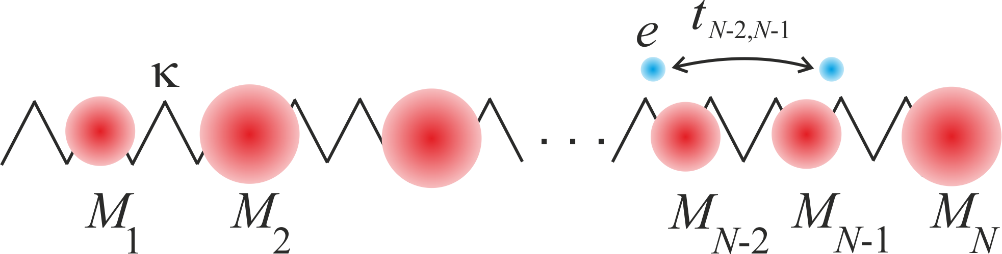
To provide a background for the following analysis of electron localization, we begin by presenting and analyzing some known results for an isotopically disordered chain with atoms (see Fig. 1) described by the Lagrangian:
| (1) |
where is component vector of atomic displacements, and matrices
| (2) |
define the positions of isotopes with masses at the th site, and elastic force constants, respectively. For calculations with the Born - von Karman periodic boundary conditions one has
The characteristic equation yields the corresponding where numerates the eigenmodes with eigenvectors and statistical properties of the frequencies distribution obtained in the pioneering paper of Dyson Dyson . For the isotopically clean system we get ( is the phonon frequency at the Brillouin zone boundary, and is the lattice constant of the chain) with and , here is the position of the th site. The orthogonality and normalization condition reads as
The operator of the displacement vector in the second quantization form is given by
| (3) |
where are the Bose annihilation and creation operators, is the average mass of atoms in a chain and normalized now includes dimensionless prefactor . To consider electron scattering by phonon modes one also needs the Fourier transformation
| (4) |
where is obtained from eigenvectors as
| (5) |
Here we consider a realization with identical isotope impurities of masses being smaller than the mass of other atoms in the chain. For a single isolated isotope there exists one vibrational mode that splits off from the continuous spectrum of phonons to form a bound state localized nearby Kosevich . For a small (we restrict our consideration below to this realistic approximation) the frequency of this mode lies slightly above .
The localized mode centered at is described by Kosevich
| (6) |
Here is the mode localization length. The resulting Fourier structure of the isotope-related mode being localized and centered at the Brillouin zone boundaries where , can be presented, assuming in the Lorentzian form as:
| (7) | |||
Since is symmetric, the Fourier component is real. The Fourier distribution of the localized mode has the width .
To characterize spatial localization of the modes we use the inverse participation ratio (IPR)
| (8) |
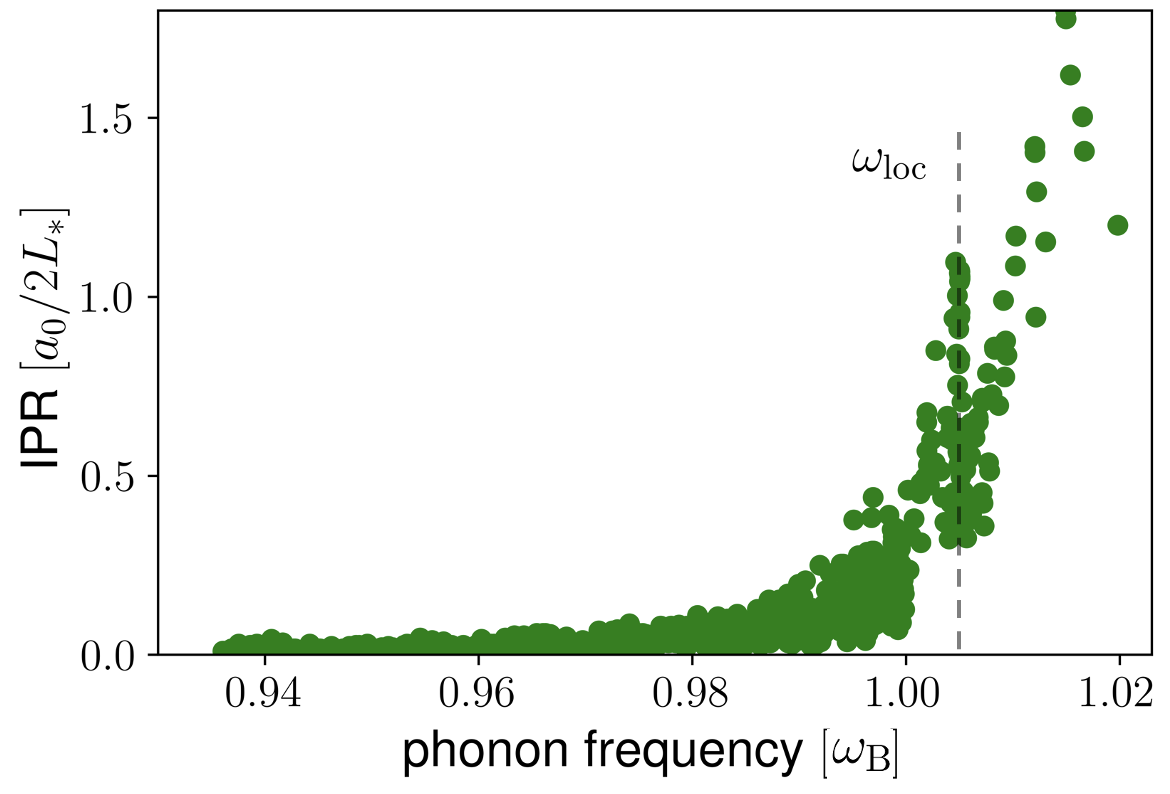
where for delocalized modes . A single isotope impurity produces a localized mode with Other phonons are delocalized with the corresponding and do not have a smooth Fourier structure. In Fig. 2 we present the for diluted disordered system where the mean distance between the light isotopes This Figure shows a clear distinction between localized and delocalized modes. It is interesting to mention that the mapping of phonon localization Dorokhov ; Dorokhov2 on the Anderson localization Anderson and the Green’s function analysis Nieuwenhuizen similar to Halperin show that at a finite concentration of impurities low-frequency phonon modes are localized, albeit with a vanishing in the zero-energy limit (see Ref. Hodges for review).
Also, Fig. 2 indicates the presence of states with frequencies and larger , suggesting smaller localization lengths. These states arise from isotopes located at the distances of the order of or less than Here we consider two identical isotope impurities and for a qualitative analysis present the displacement as and use a continual model Kosevich for the envelope function with impurities presented as potentials at distance
| (9) |
where is the speed of sound, resulting in the equation for
| (10) |
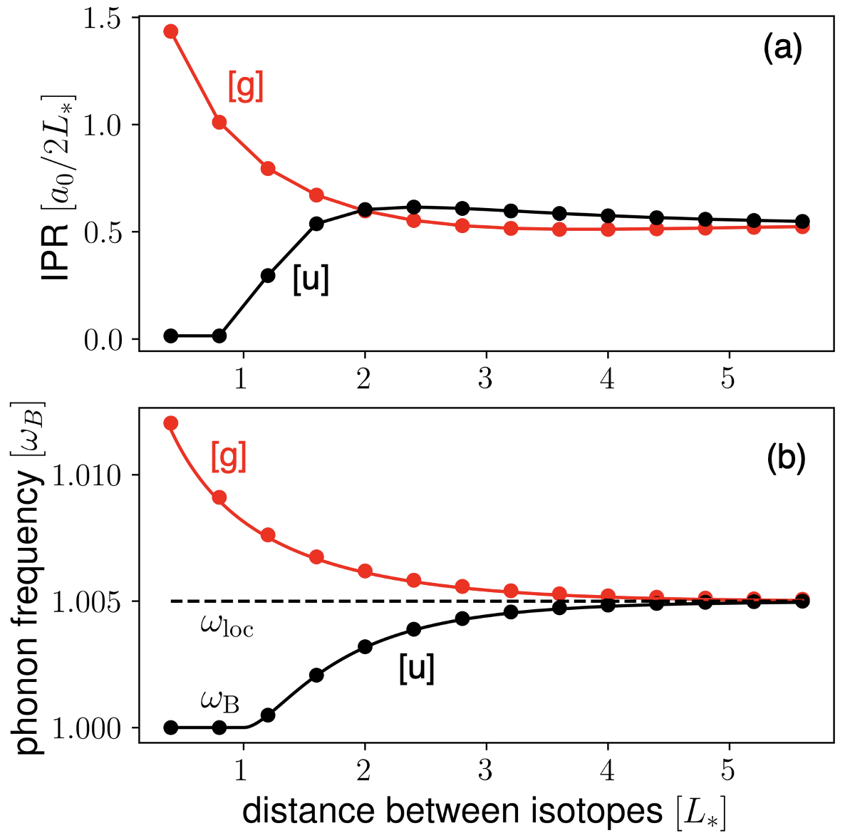
with and
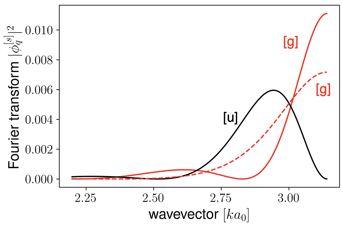
Equation (10) implies that at a sufficiently small distance between the isotopes only one (even) mode remains localized with while the other, odd one , is pushed into the phonon continuum and becomes delocalized. These features are shown in Fig. 3, where we present the dependence of and its on the distance between the isotopes. The corresponding Fourier components given by Eq. (5) are presented in Fig. 4.
II.2 Electron-phonon interaction
We present the electron Hamiltonian in the tight binding form
| (11) |
with the bond-dependent hopping (see Fig. 1) , with being the electron annihilation and creation operators (irrelevant spin degrees of freedom are not included). In the electron momentum basis the phonon-independent term determines the one-dimensional electron dispersion . The non-interacting part of the Hamiltonian is given by
| (12) |
The electron-phonon interaction part can be written as
| (13) |
where is given by Eq. (4) with and the form factor It is also convenient to rewrite the interaction potential in the form that directly exploits
| (14) |
the electron-phonon interaction constant , where is the deformation potential of the chain, is the mass density, and is the chain length.
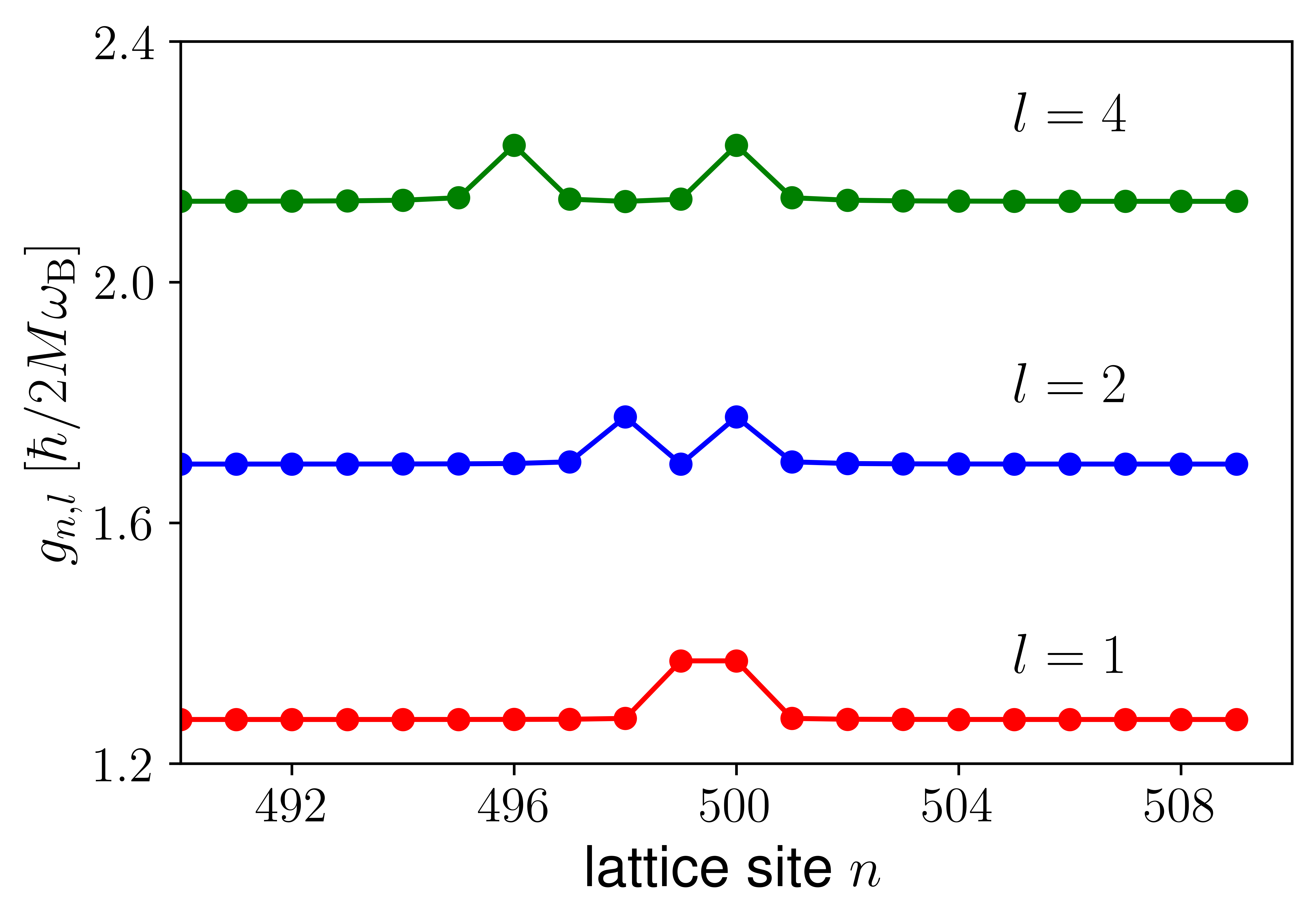
To explicitly confirm the effect of isotopic impurities on the quantum fluctuations of the intersite distances and corresponding electron hopping, we introduce the correlation function (cf. Eq. (3)):
| (15) |
Figure 5 demonstrates the dependence of (in the units of ) on the lattice site in the vicinity of the isotope for different . Though the localized phonon mode has a spatial size , this scale is not reflected in the behavior of . The latter is mainly determined by low-frequency phonons with small corrections appearing due to the mass defect at the isotope site. The increase in in the vicinity of the isotopic defect shows that the hopping integral fluctuates correspondingly and, thus can influence the electron motion. However, as we will see below, the analysis of electron scattering cannot be reduced to using the only correlation function
III Scattering and localization
III.1 Elastic scattering by localized modes
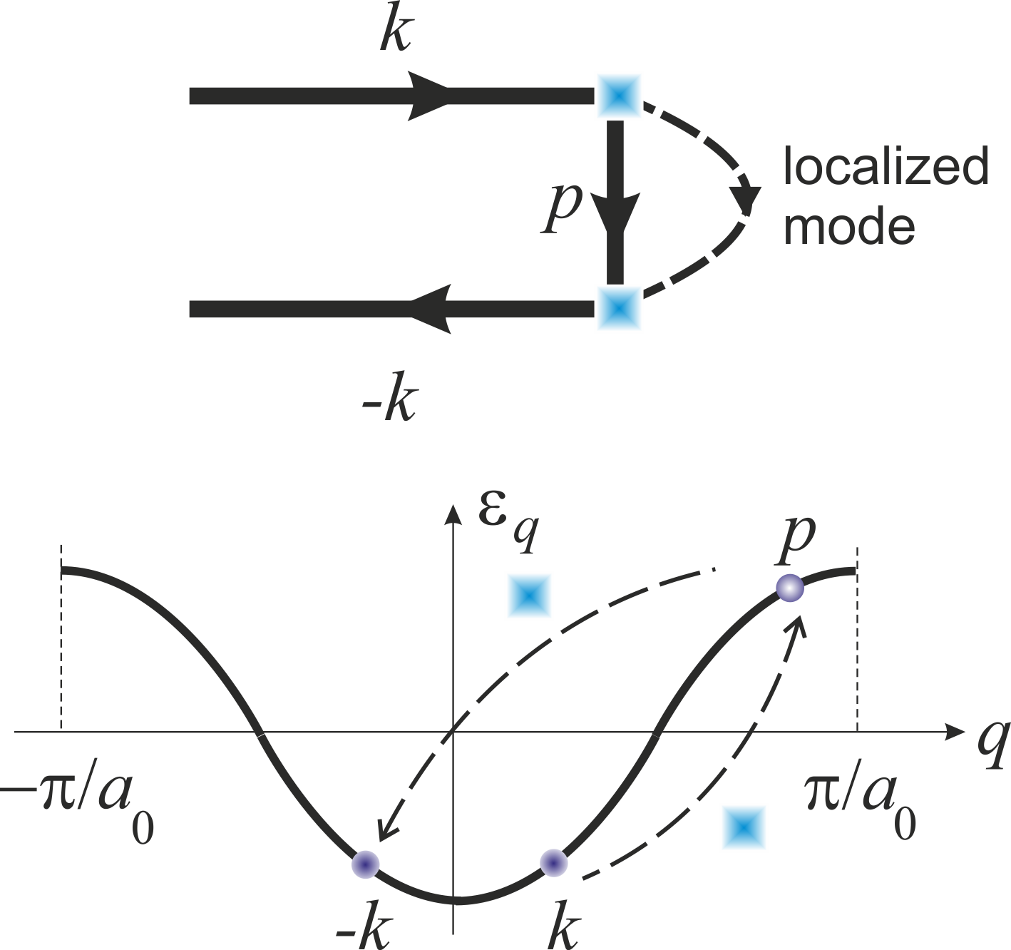
Aiming at analysis of localization we focus on the elastic electron scattering involving virtual phonon processes with the corresponding Feynman graph in Fig. 6. This process appears in the second-order with respect to and is due to the finite spread of phonon momentum in presence of isotopes. The effective potential for an electron interacting with quantum vibrations in second-order can be obtained following Refs. Luttinger ; Kittel and is given by
| (16) |
where stands for the commutator and operator is determined from By taking the matrix elements of this commutator with respect to the eigenstates of (such as where is the vacuum state), we obtain
| (17) |
To analyze the elastic scattering we first consider the matrix elements of between and phononless states. The explicit expression for this matrix element, , is
| (18) |
At small electron momenta the electron velocity and effective mass with To avoid decoherence processes related to the emission of real phonons and suppressing the electron localization, we note that the no-emission condition restricts momentum to where Notice that the condition prohibits the emission of real localized modes also. Using from Eq. (14) we keep in the sum of Eq. (III.1) only the modes corresponding to the localized states of Eq. (7) with frequency For a low concentration of single isotopes with a small mass defect, the Fourier components of other, delocalized, phonon modes with the frequencies lying within the phonon band spectrum, do not acquire a width sufficient to contribute to the sum in Eq. (III.1). Thus, we arrive at the matrix element of the electron scattering by a single isotope impurity:
| (19) | |||

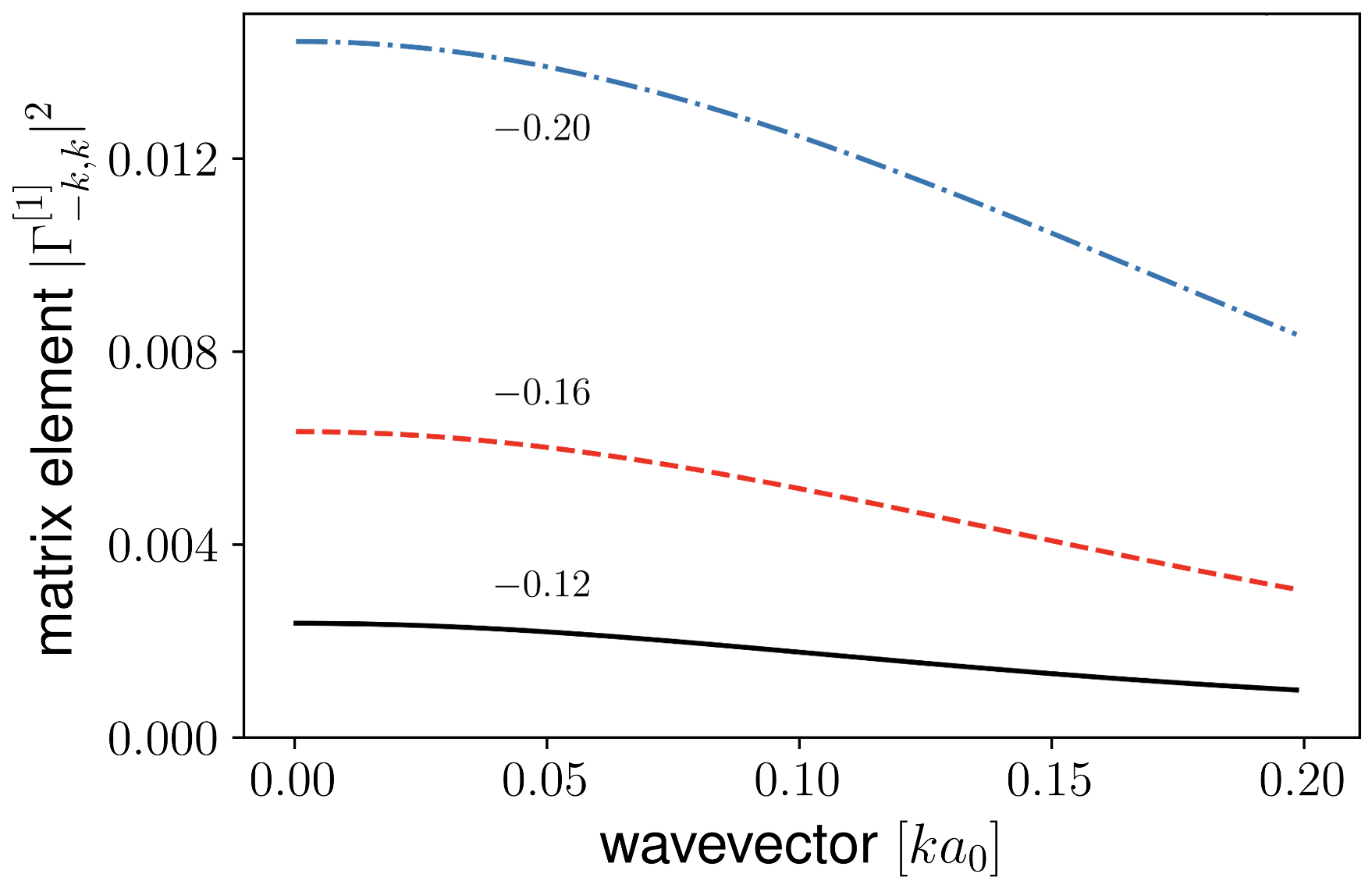
The plot of corresponding to presented in Fig. 7 demonstrates that the scattering matrix element is relatively large only in the range. The resulted calculated weakness of backscattering is due to two factors: a small allowed momentum transfer with , arising from the , see Eq.(7), and small at small and . By using the condition and expression for in Eq. (7), we obtain:
| (20) |
In the limit behaves as and decreases as at Equations (19) and (20) present the key result of this paper: Quantum isotopic impurities characterized by localized finite-frequency phonon modes can produce elastic electron backscattering. The corresponding numerically calculated is presented in Fig. 8.
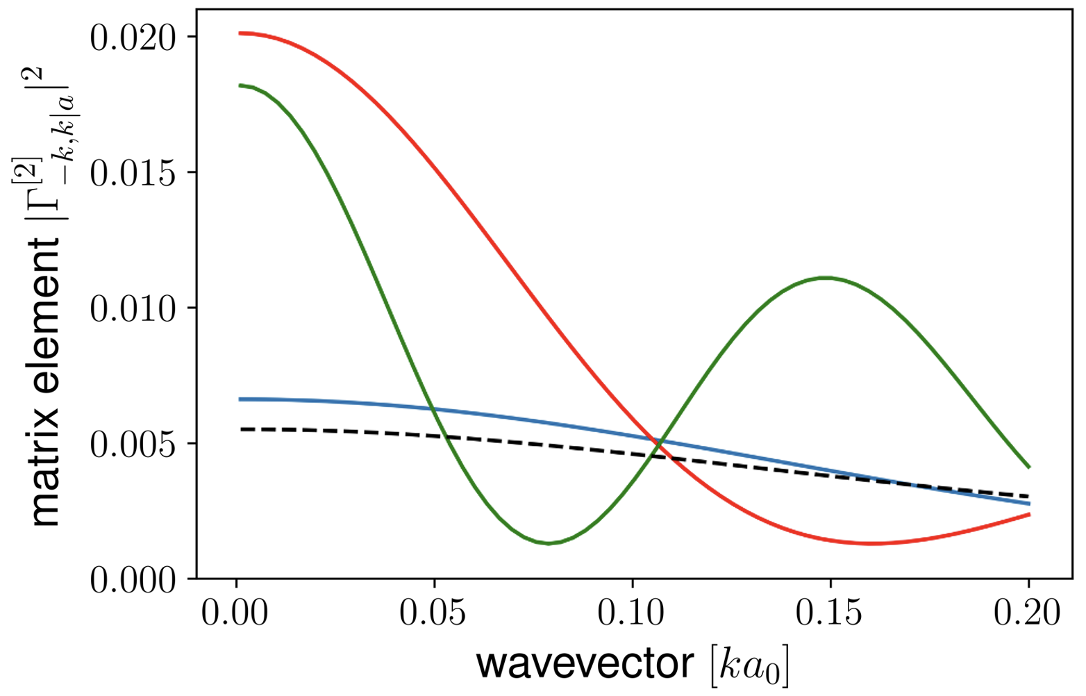
Having demonstrated possible elastic scattering by a single isotopic impurity, we can study how this general approach can be applied for two closely related impurities, where interference of scatterings by odd and even vibrational modes plays a qualitative role, and see the characteristic features of this scattering. The matrix element of backscattering by two-isotope states, corresponding to Figs. 3 and 4, has the form:
| (21) | |||
and shows interference of the scattering processes. The corresponding probabilities are presented in Fig. 9. It is worth mentioning an increase in the scattering probability when two isotopes are located at , indicating a stronger scattering.
III.2 Low density of impurities: possible single-impurity localization and free path
As we demonstrated in the previous subsection, at small isotopic defects concentrations, a disordered chain can be presented as a randomly spaced ensemble of elastic scatterers, corresponding to scattering by a single and pairs of isotopic impurities. We assume a sufficiently small concentration of isotope impurities such that they behave as independent single scatterers located at uncorrelated points The resulting small concentration of isotope pairs of the order of does not modify the localization-related results.
We begin with the quantum mechanical analysis of the electron free path in this system, where the finite free path indicates localization behavior and assuming that the main effect is due to single scatterers. In this analysis we use the one-dimensional free space electron Green’s function in the form:
| (22) |
where Using the Green function from Eq. (22) we obtain in the first Born approximation for scattering by a single isotope impurity located at a point :
| (23) | |||
where and one expects as the approximation validity condition. The sign of is negative corresponding to an attractive potential of the width depth of the order of and the binding energy of the order of Here we used relations to scale the energy in dimensionless units and by assuming that the intersite hopping integral is sufficiently modified at the modulation in the interatomic distance of the order of (cf. Eq. (14)).
In the positive energy domain, the mean free path due to back scattering by isotopes can be estimated as corresponding to the Anderson localization at the spatial scale of the order of Indeed is very small almost in the entire interval of at the energies At smaller energies, approaches 1 and more detailed scattering approaches Halperin ; Azbel have to be applied. To characterize the scattering, one can introduce dimensionless parameters and where, due to the condition the parameter represents the upper limit of the scattering time. Although can be either smaller or greater than 1, the product is always much larger than 1. This implies that scattering by isotopic impurities is an adiabatic process with low probability due to averaging of the intersite hopping during the scattering leading as a result to the adiabatic limit for the binding energy
III.3 Electron localization
Here we concentrate on electron localization by using the result of previous subsections on mapping of isotopic impurities in chains on weak scatterers of electrons. As it is was shown in Ref. Berry , one-dimensional arrays of random scatterers lead to the localization of light waves with the same approach valid for the localization of electron waves.
Several approaches including the Lyapunov exponents analysis (e.g., Gurevich2011 ) and random matrix theory (e.g., Beenakker1997 ) can be used for studies of wave localization in random potentials. We will use a direct numerical calculation proving electron localization by producing a random potential corresponding to isotopic scatterers and calculating electron eigenstates in this potential. To study the localization we consider a normalized electron wavefunction on a sites one-dimensional lattice, where enumerates the lattice sites and enumerates the electron states with the energies The probability density distribution for the state is characterized by the corresponding inverse participation ratio:
| (24) |
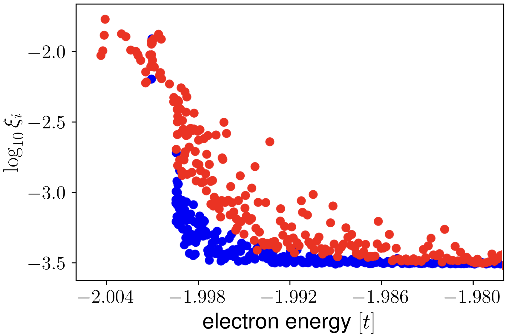
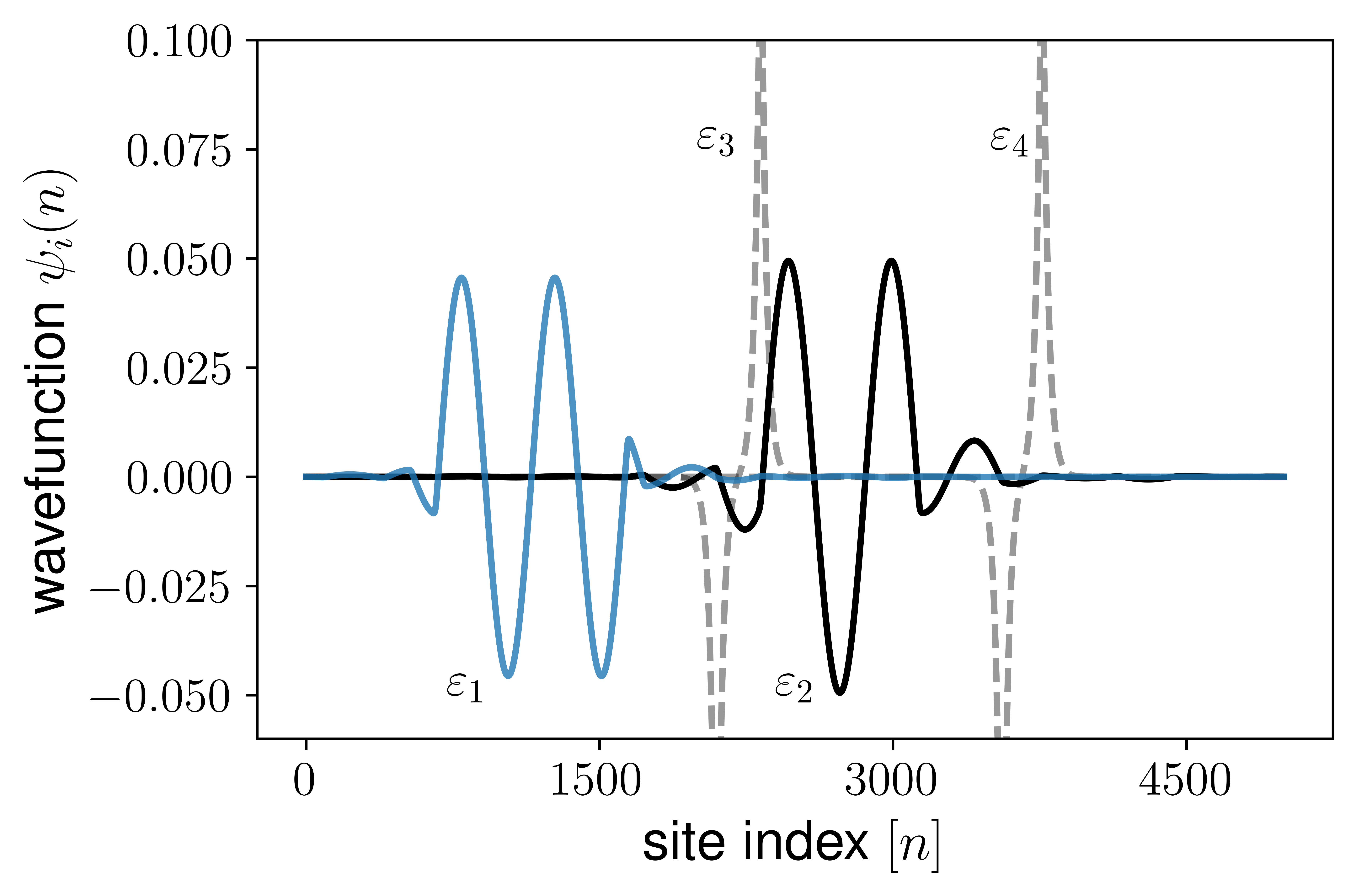
The results for presented in Fig. 10 demonstrate the formation of two groups of localized states. The first group corresponds to the impurity band formed below the bottom of the conduction band with Lifshitz_book . The second group corresponds to the Anderson localization of the states inside the conduction band with We notice that, as expected, the states become delocalized at the energies corresponding to where the backscattering probability is strongly suppressed, according to Eq. (23) and Eq. (20), where behaves as rapidly decreasing with the electron energy. Further, in Fig. 11 we present several typical wavefunctions demonstrating that the Anderson localization occurs on a spatial scale much larger than the distance between the isotopic impurities.
Finally, we emphasize that our approach is qualitatively different from that proposed in Refs. Berezin1982 ; Berezin1984a ; Berezin1984b ; Berezin1987 . The analysis in these papers is based on the fact that the electron self energy due to electron-phonon coupling, producing bandgap renormalization, is proportional to the dependent on the atomic masses mean inverse phonon frequency Kittel . Thus, clusters of isotopic impurities with sufficiently large size and concentration, renormalizing locally the electron bandgap, can produce effective “potentials” able to localize sufficiently heavy carriers. Our approach is unrelated to the bandgap renormalization and electron localization occurs do to elastic scattering by randomly distributed localized phonon modes.
IV Conclusions and outlook
We studied the localization of electrons due to a weak isotopic disorder producing randomly spatially distributed localized phonon modes in one-dimensional systems described by a tight-binding model. Elastic electron scattering involving nonlocal processes of virtual emission and absorption of these modes is presented in the form of scattering by a weak potential with a strongly energy-dependent reflection probability. This randomness, related to the virtual phonon emission and absorption processes leads to the Anderson localization with the localization length dependent on the electron energy. Investigations of more complex realizations including the formation of random weak coupling polarons due to a strong isotopic disorder and possible effects of lattice nonlinearity (see, e.g. Ref. Savin ) are of interest and will be a topic of future research.
To conclude the discussion of the effect of isotopic mass on the electron position in systems with different isotopes that emphasizes its general character, we mention that this effect is related to the puzzling dipole moment of the HD molecule Trefler , where different amplitudes of zero-point vibrations of hydrogen and deuterium ions lead to a shift of the electron probability density between these atoms resulting in the formation of a small dipole moment Trefler ; Blinder .
V Acknowledgements
The work of E.S. is supported through Grants No. PGC2018-101355-B-I00 and No. PID2021-126273NB-I00 funded by MCIN/AEI/10.13039/501100011033 and by the ERDF “A way of making Europe”, and by the Basque Government through Grant No. IT1470-22. E.S. is grateful to C. Draxl, N. Protik, J.E. Sipe, and V.A. Stephanovich for valuable discussions.
References
- (1) I. Ya. Pomeranchuk, Isotopic Effect in the Residual Electrical Resistance of Metals, Sov. Phys. JETP 8, 693 (1959)
- (2) Yu. M. Kagan and A. P. Zhernov, Electrical Conductivity of Isotopically Disordered Metals, Sov. Phys. JETP 26, 999 (1968).
- (3) N. Vandecasteele, M. Lazzeri, and F. Mauri, Boosting Electronic Transport in Carbon Nanotubes by Isotopic Disorder, Phys. Rev. Lett. 102, 196801 (2009).
- (4) V. L. Berezinskii, Kinetics of a Quantum Particle in a One-Dimensional Random Potential, Sov. Phys. JETP 38, 620 (1974).
- (5) N. Kumar, D. V. Baxter, R. Richter, and J. O. Strom-Olsen, Weak Localization in Two and Three Dimensions: Dephasing by Zero-Point Motion, Phys. Rev. Lett. 59, 1853 (1987).
- (6) J. Rammer, A. L. Shelankov, and A. Schmid, Comment on ”Weak Localization in Two and Three Dimensions: Dephasing by Zero-Point Motion” Phys. Rev. Lett. 60, 1985 (1988).
- (7) G. Bergmann, Comment on ”Weak Localization in Two and Three Dimensions: Dephasing by Zero-Point Motion” Phys. Rev. Lett. 60, 1986 (1988).
- (8) M. M. Glazov, Z. A. Iakovlev, and S. Refaely-Abramson, Phonon-induced exciton weak localization in two-dimensional semiconductors, Appl. Phys. Lett. 121, 192106 (2022).
- (9) A. A. Gogolin, V. I. Mel’nikov, and E. I. Rashba, Conductivity in a Disordered One-Dimensional System Induced by Electron-Phonon Interaction, Sov. Phys. JETP, 42, 168 (1975).
- (10) L. Borda, L. Fritz, N. Andrei, and G. Zaránd, Theory of inelastic scattering from quantum impurities, Phys. Rev. B 75, 235112 (2007).
- (11) F. J. Dyson, The Dynamics of a Disordered Linear Chain, Phys. Rev. 92, 1331 (1953).
- (12) I. M. Lifshitz and G.I. Stepanova, Vibration spectrum of disordered crystal lattices, Sov. Phys. JETP 3, 656 (1956).
- (13) I. M. Lifshitz, Energy spectrum structure and quantum states of disordered condensed systems, Sov. Phys.-Usp. 7, 549 (1965).
- (14) A. Maradudin and G. H. Weiss, The Disordered Lattice Problem: A Review, Journal of the Society for Industrial and Applied Mathematics, 6, 302 (1958).
- (15) A. A. Maradudin, E. W. Montroll, and G. H. Weiss, Theory of lattice dynamics in the harmonic approximation (Academic Press, Lomdon, UK, 1963)
- (16) I. M. Lifshits, S. A. Gredeskul, and L. A. Pastur, Introduction to the Theory of Disordered Systems (Wiley-VCH, Hoboken, NJ, US, 1988).
- (17) W. R. Mondal, N. S. Vidhyadhiraja, T. Berlijn, J. Moreno, and M. Jarrell, Localization of phonons in mass-disordered alloys: A typical medium dynamical cluster approach, Phys. Rev. B 96, 014203 (2017).
- (18) N. H. Protik and C. Draxl, Beyond the Tamura model of the phonon-isotope scattering, Phys. Rev. B 109, 165201 (2024).
- (19) A. M. Kosevich, The Crystal Lattice: Phonons, Solitons, Dislocations, Superlattices, (2005).
- (20) O. N. Dorokhov, Localization of the Phonon Modes in a Disordered Elastic Chain, Sov. Phys. JETP 56, 128 (1982).
- (21) O. N. Dorokhov, Absence of quantum diffusion in a disordered elastic chain, Solid State Commun. 41, 431 (1982).
- (22) P. W. Anderson, Absence of Diffusion in Certain Random Lattices, Phys. Rev. 109, 1492 (1958).
- (23) Th. M. Nieuwenhuizen and M. H. Ernst, Transport and spectral properties of strongly disordered chains, Phys. Rev. B 31, 3518 (1985).
- (24) B. I. Halperin, Green’s Functions for a Particle in a One-Dimensional Random Potential, Phys. Rev. 139, A104 (1965).
- (25) C. H. Hodges and J. Woodhouse, Theories of noise and vibration transmission in complex structures, Rep. on Progress in Physics 49, 107 (1986).
- (26) J.M. Luttinger and W. Kohn, Motion of Electrons and Holes in Perturbed Periodic Fields, Phys. Rev. 97, 869 (1955).
- (27) C. Kittel, Quantum Theory of Solids, Wiley (1991).
- (28) M. Ya. Azbel, Eigenstates and properties of random systems in one dimension at zero temperature, 28, 4106 (1983).
- (29) M.V. Berry and S. Klein, Transparent mirrors: rays, waves and localization, Eur. J. Phys. 18, 222 (1997).
- (30) E. Gurevich and A. Iomin, Generalized Lyapunov exponent and transmission statistics in one-dimensional Gaussian correlated potentials, Phys. Rev. E 83, 011128 (2011).
- (31) C. W. J. Beenakker, Random-matrix theory of quantum transport, Rev. Mod. Phys. 69, 731 (1997).
- (32) A.A. Berezin, Localized States Associated with Isotopic Islands, J. Phys. Chem. Solids 48, 853 (1987).
- (33) A.A. Berezin, Anderson localization induced by an isotopic disorder, Lett. Nuovo Cimento 34, 93 (1982).
- (34) A.A. Berezin, An isotopic disorder as a possible cause of the intrinsic electronic localization in some materials with narrow electronic bands, J. Chem. Phys. 80, 1241 (1984).
- (35) A.A. Berezin, Isotopic disorder as a limiting factor for the mobility of charge carriers, Chem. Phys. Lett. 110, 385 (1984).
- (36) A. V. Savin, Y.S. Kivshar, and M.I. Molina, Disorder-free weak dynamic localization in deformable lattices, J. Phys.: Condens. Matter 30, 375602 (2018).
- (37) M. Trefler and H. P. Gush, Electric Dipole Moment of HD, Phys. Rev. Lett. 20, 703 (1968).
- (38) S.M. Blinder, Dipole Moment of HD, J. Chem. Phys. 32, 105 (1960).