ShapeSplat: A Large-scale Dataset of Gaussian Splats and Their Self-Supervised Pretraining

Abstract

3D Gaussian Splatting (3DGS) has become the de facto method of 3D representation in many vision tasks. This calls for the 3D understanding directly in this representation space. To facilitate the research in this direction, we first build a large-scale dataset of 3DGS using the commonly used ShapeNet and ModelNet datasets. Our dataset ShapeSplat consists of 65K objects from 87 unique categories, whose labels are in accordance with the respective datasets. The creation of this dataset utilized the compute equivalent of 2 GPU years on a TITAN XP GPU.

We utilize our dataset for unsupervised pretraining and supervised finetuning for classification and segmentation tasks. To this end, we introduce Gaussian-MAE, which highlights the unique benefits of representation learning from Gaussian parameters. Through exhaustive experiments, we provide several valuable insights. In particular, we show that (1) the distribution of the optimized GS centroids significantly differs from the uniformly sampled point cloud (used for initialization) counterpart; (2) this change in distribution results in degradation in classification but improvement in segmentation tasks when using only the centroids; (3) to leverage additional Gaussian parameters, we propose Gaussian feature grouping in a normalized feature space, along with splats pooling layer, offering a tailored solution to effectively group and embed similar Gaussians, which leads to notable improvement in finetuning tasks. Our code will be available at ShapeSplat.

Abstract

This supplementary material first provides the nomenclature of our method for reference, followed by further information for better reproducibility as well as additional evaluations and qualitative results.

1 Introduction

3D Gaussian Splatting [22], a recent advancement in radiance field that represents 3D scenes using Gaussian primitives, has garnered significant research interest beyond view synthesis task, including scene reconstruction and editing [57, 65], segmentation and understanding [60, 43], digital human [42, 23], and 3D generation [62, 49].

Gaussian splats representation offers numerous advantages, including rapid rendering speeds, high fidelity, differentiability, and extensive editability. These features establish 3D Gaussian Splatting as a potential game changer for encoding the scenes in 3D vision pipelines.

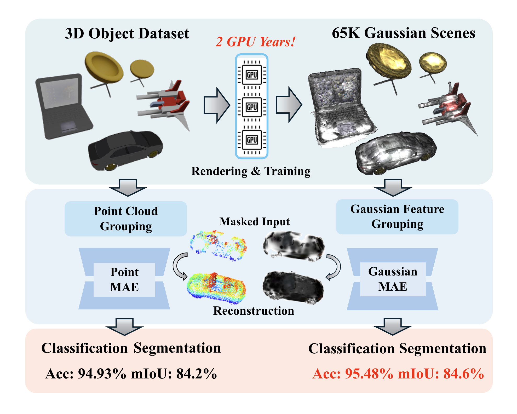
Figure 1: ShapeSplat Dataset and Gaussian-MAE. We present ShapeSplat, a large-scale dataset that took 2 GPU years to render and rasterize. Thanks to the dataset and the proposed pretraining method Gaussian-MAE, we outperform the point cloud counterpart method by 0.55$\%$ in accuracy and 0.4$\%$ in mean IoU.

To the best of our knowledge, there has been no exploration of direct learning on trained parameters of Gaussian splats in current research. A significant barrier in this regard is the lack of a large-scale dataset of trained Gaussian Splatting scenes. Despite 3DGS having considerably reduced the computation time, generating such a large-scale dataset remains significantly time-consuming. This paper seeks to address this challenge with the ShapeSplat dataset, which comprises over 65K Gaussian splatted objects across 87 different categories. The dataset is designed to facilitate research in self-supervised pretraining of Gaussian splats, and to support downstream tasks, including classification, and 3D part segmentation, as shown in Fig. 1.

With this large-scale dataset, we first perform unsupervised pretraining in a masked autoencoder manner [17], followed by supervised finetuning for classification and segmentation tasks. Our extensive experiments demonstrate that each Gaussian parameter—opacity, scale, rotation, and spherical harmonics—can be effectively reconstructed during the pretraining stage. Moreover, incorporating additional Gaussian parameters notably enhances performance in downstream tasks.

We apply our model (pretrained on Gaussian centroids) to the uniformly sampled point clouds, showcasing its generalizability. We observed that while using Gaussian centroids alone is sufficient for the segmentation task, it leads to a performance drop in the classification task. This might be due to the complex spatial distribution of Gaussian parameters, as Gaussians tend to have larger scales and higher opacity in planar regions, while in corners and edges, they appear with smaller scale and opacity, as shown in Fig. 3. To address this, we propose a Gaussian feature grouping technique and splats pooling layer, whose effectiveness is demonstrated in pretraining and finetuning.

In summary, our key contributions are as follows:

$\bullet$ We present ShapeSplat, a large-scale Gaussian splats dataset spanning 65K objects in 87 unique categories.

$\bullet$ We propose Gaussian-MAE, the masked autoencoder based self-supervised pretraining for Gaussian splats, and analyze the contribution of each Gaussian attribute during the pretraining and supervised finetuning stages.

$\bullet$ We propose novel Gaussian feature grouping with splats pooling layer during the embedding stage, which are customized to the Gaussian splats’ parameters, enabling better reconstruction and higher performance respectively.

2 Related Work

2.1 3D Object Datasets

Since the rapid advancement of 3D deep learning, despite the challenges of collecting, annotating, and storing 3D data, significant progress has been made in 3D datasets [10, 13, 34, 38, 4, 68, 3, 56, 54, 5, 6, 50] in recent years, thanks to the dedicated efforts of the community. ShapeNet [3] has been a foundational platform for modeling, representing, and understanding 3D shapes in 3D deep learning. It offers over 3 million textured CAD models, with a subset called ShapeNet-Core containing 52K models, organized by mesh and texture quality. Similarly, ModelNet [56] provides 12K CAD models, while OmniObject3D [54] includes 6K objects with more category variation. To further scale up, efforts like Objaverse [5] and Objaverse-XL [6] have been introduced, containing 800K and 10.2 million models respectively and with rich text annotation, significantly accelerating research in large-scale 3D understanding. We selected ShapeNet [3] as our choice for a pretrained Gaussian splats dataset due to its extensive size. For validation datasets in classification and 3D segmentation tasks, we chose ModelNet and ShapeNet-Part [61]. Additionally, we included ScanObjectNN [50] for real-world applications. These choices were made because they offer similar categories and provide well-established benchmarks for 3D deep learning methods. Related to our work, [20, 31] build NeRF [32] representation on ScanNet and Omniobject3D. Instead, we use Gaussian splats as 3D representation.

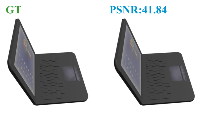
(a) Laptop

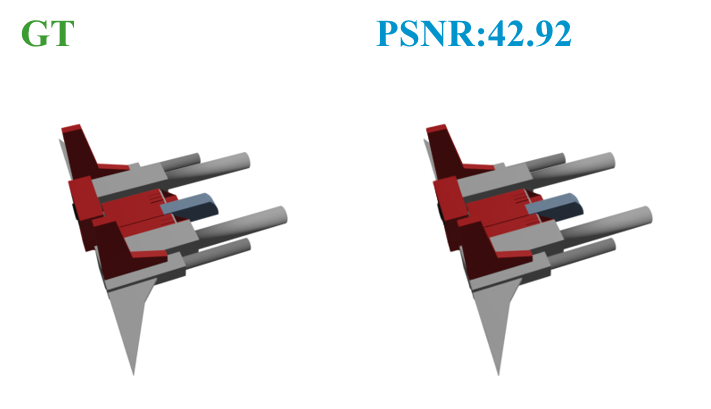
(b) Airplane

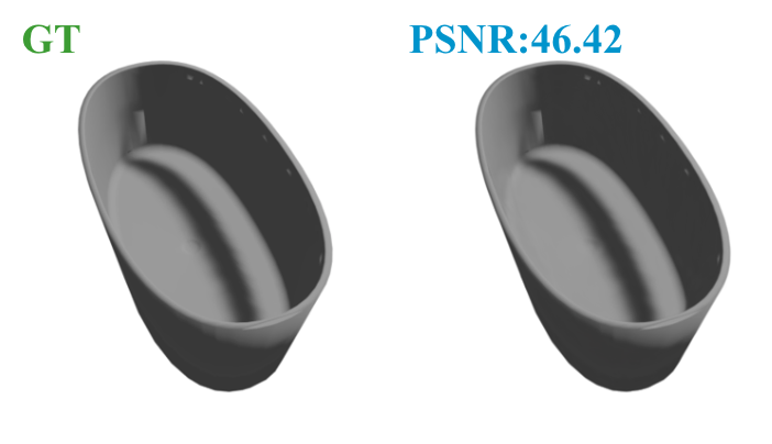
(c) Bathtub

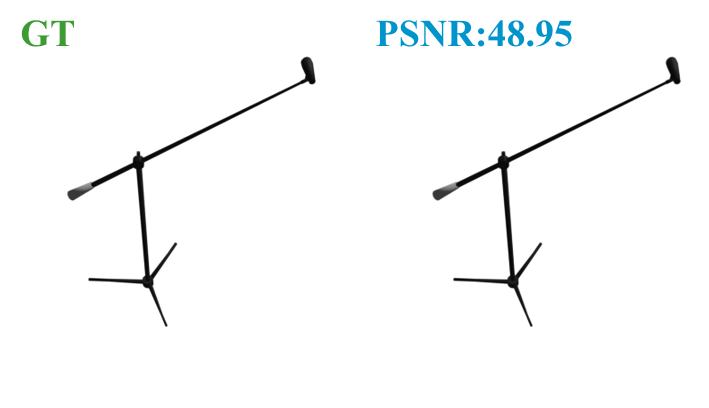
(d) microphone

Figure 2: Qualitative Results of ShapeSplat Rendering. We present high quality renderings used for ShapeSplat on complex surfaces, shadows, and thin objects.

Dataset	ShapeNet-Core	ShapeNet-Part	ModelNet
Task	Classification	Segmentation	Classification
Category	55	50	40
Objects	52,121	16,823	12,308
GPU(days)	548.41	175.23	51.03
Gaussians	24,267	23,689	22,456
PSNR	44.187	44.542	45.104
JSD[70]	0.231	0.207	0.230
MMD[70]	0.137	0.087	0.135

Table 1: Dataset Statistics. We provide the specifications for the proposed ShapeSplat dataset, highlighting its quality and difference from the initial datasets in spatial distribution and the substantial preparation effort involved.

2.2 Gaussian Splatting

A plethora of research has focused on achieving better rendering quality, real-time speed, and scene editability with the advent of neural radiance fields, yet none have successfully addressed all these aspects. Building upon the rasterization technique, Kerbl et al. [22] proposed to represent the scene with a set of 3D Gaussian primitives, which significantly increased the rendering speed and obtained state-of-the-art rendering quality. Inspired by the success of 3D Gaussian Splatting (3DGS), a surge of following works further improve the rendering quality, geometry, and scene compression, extend to dynamic tasks, and utilize it as the representation bridging images and 3D scenes.

To represent accurate surface geometry, [16, 19, 65] have introduced a rasterized method for computing depth and normal maps based on the Gaussian splats, and apply regularization for better surface alignment. Research on Gaussian scene compression [33, 35] utilized a learnable mask strategy or vector clustering technique to reduce total parameters without sacrificing rendering performance. Some works [30, 59, 24, 14] extended the 3D Gaussians to dynamic scenes and deformable fields by explicitly modeling the Gaussians across time steps or using a deformation network to decouple the motion and geometry structure. Attracted by the efficiency of 3DGS, [1, 64, 47] explored its optimization capability on re-rendering for pose estimation and mapping tasks. Researchers also have combined 3DGS with diffusion models to achieve efficient inpainting [28] and text-to-3D generation [48, 62]. Furthermore, there were efforts to lift 2D features from foundation models to attributes of Gaussian primitives [43, 69], enabling language-driven probes and open-world scene understanding. Unlike these methods, our pipeline explores the rich information encoded in the Gaussian parameters without using any external features or supervision.

2.3 Self-supervised 3D Representation Learning

Self-supervised learning (SSL) has gained traction in computer vision due to its ability to generate supervisory signals from data itself [15, 17, 2]. In 3D representation learning, SSL methods using Vision Transformers (ViTs) [52, 9, 44] are also advancing. These methods generally fall into two categories: contrastive and generative approaches. Contrastive pretraining focuses on learning discriminative representations to differentiate between samples, but applying this to ViTs-based 3D pretraining is challenging due to issues like overfitting and mode collapse [41, 45]. In contrast, generative pretraining, inspired by the mask and reconstruct strategy from BERT [7] and adapted to vision as masked autoencoder (MAE) [17], has been extended to 3D by targeting point clouds [36, 66], meshes [26], or voxels [18].

On this road, several works have advanced 3D representation learning by tailoring model architectures to specific input modalities, such as point clouds and voxel grids. Zhao et al. [67] developed self-attention layers for point clouds that are invariant to permutations and cardinality. Yang et al. [58] adapted the Swin Transformer [27] for voxel grids, enabling scalability to large indoor scenes. Building on these architectures, some studies have explored encoding features from various scene representations using SSL. For instance, Yu et al. [66] utilized a standard transformer and BERT-style pretraining with dVAE [46] for point patches. Irshad et al. [21] applied MAE pretraining on Neural Radiance Fields, which enhanced scene-level tasks but faced challenges with scalability and data preparation. To the best of our knowledge, there is no prior work exploring the representation of trained 3D Gaussian splats parameters.

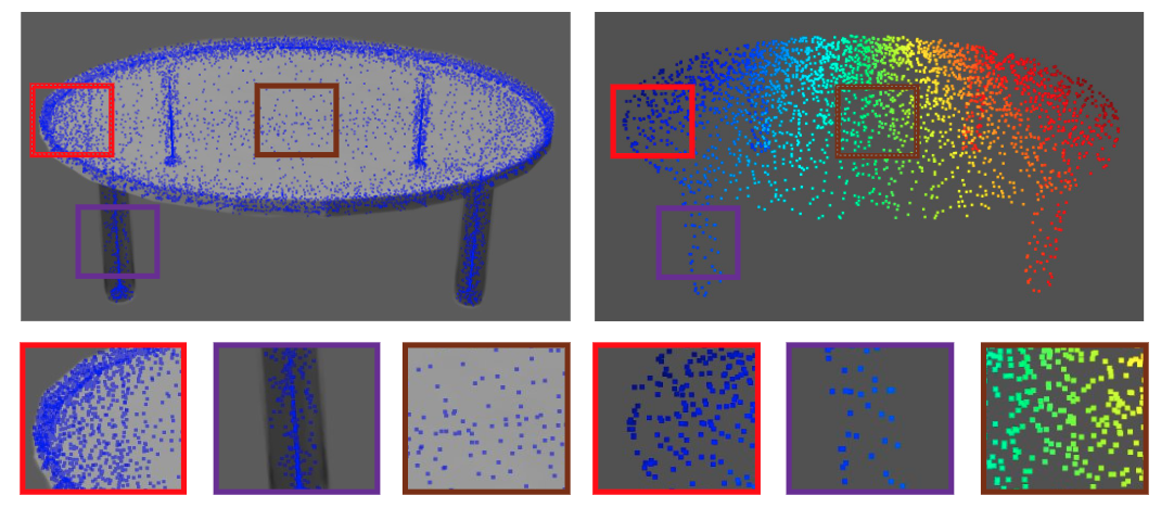
Figure 3: Distribution Comparison of Gaussian Splats Centroid and Point Cloud. We highlight the difference of Gaussian centroids (left) and the point cloud used for initialization (right).

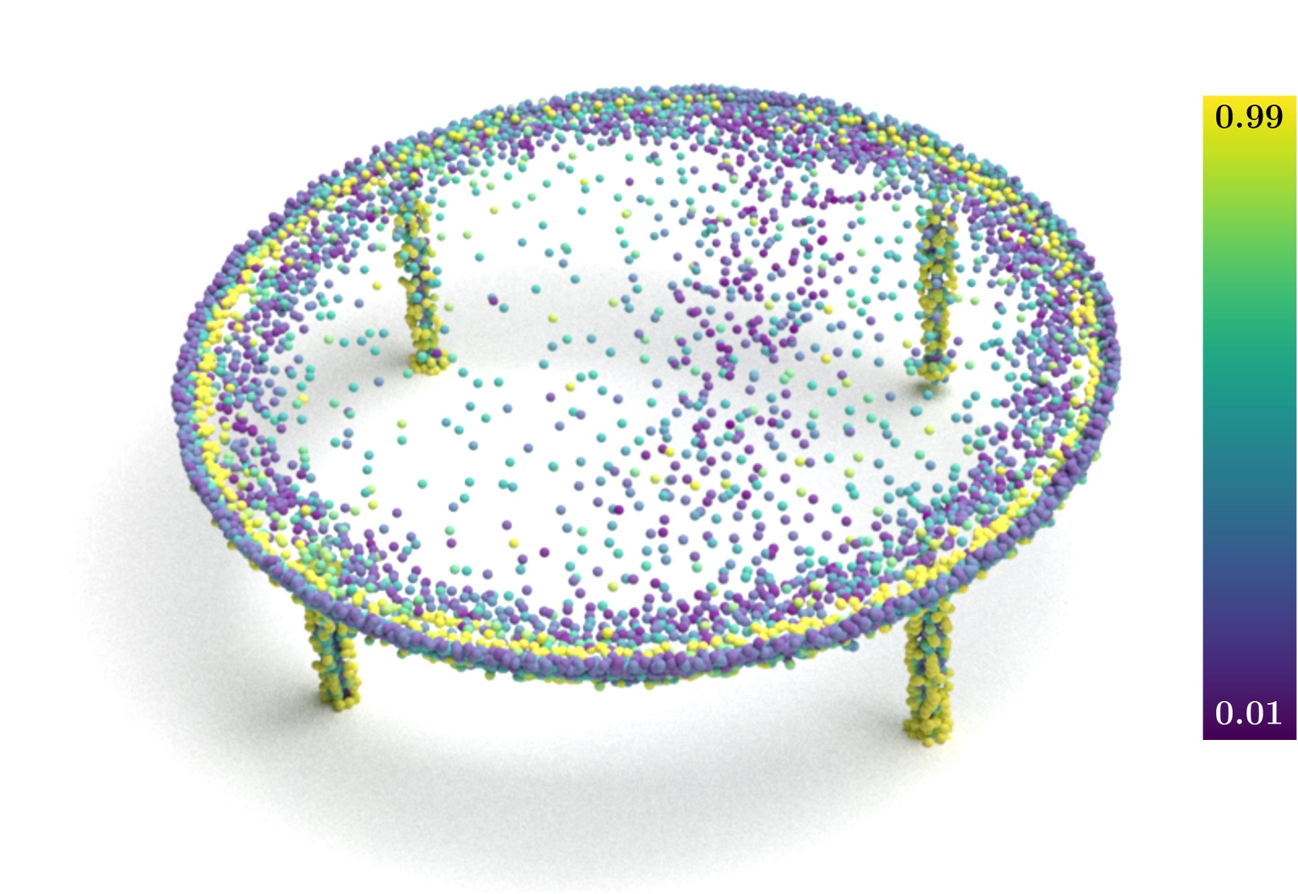
(a) Opacity

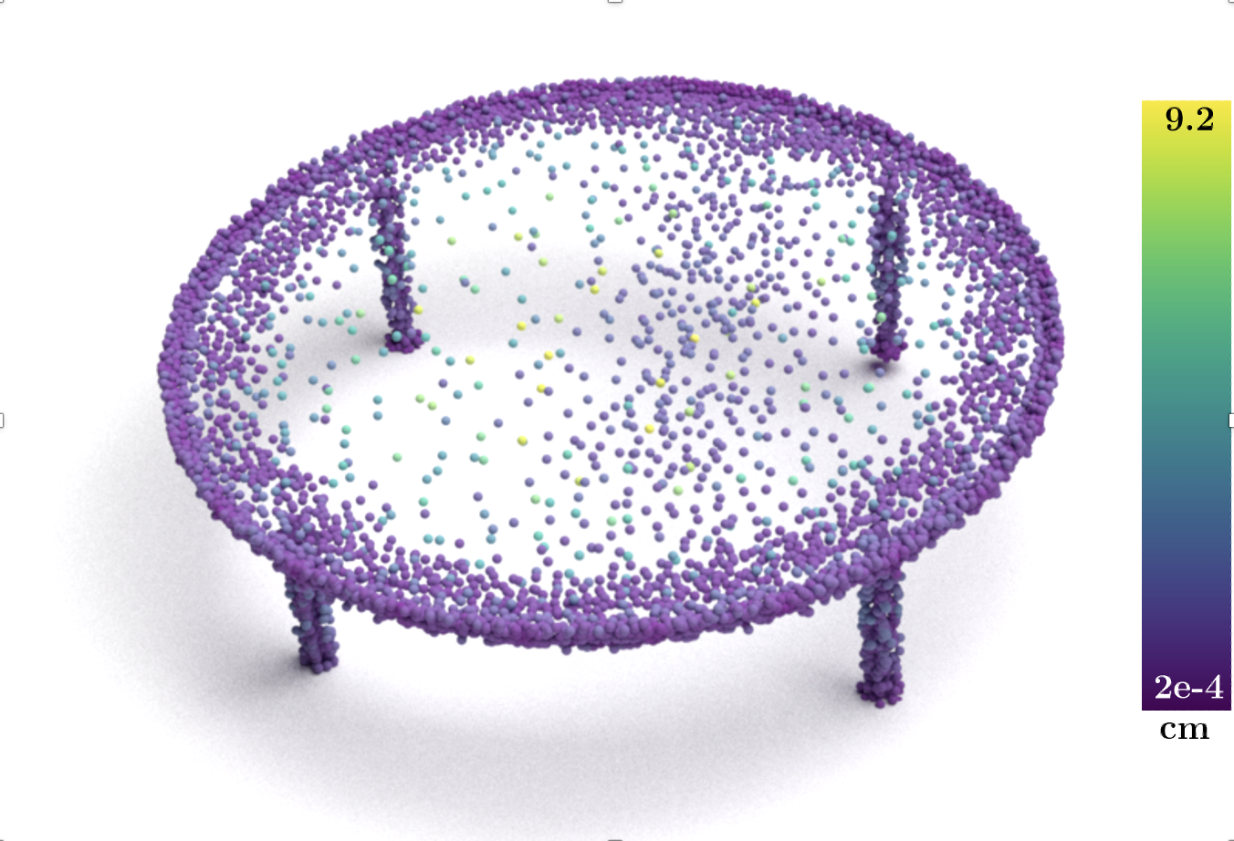
(b) Scale

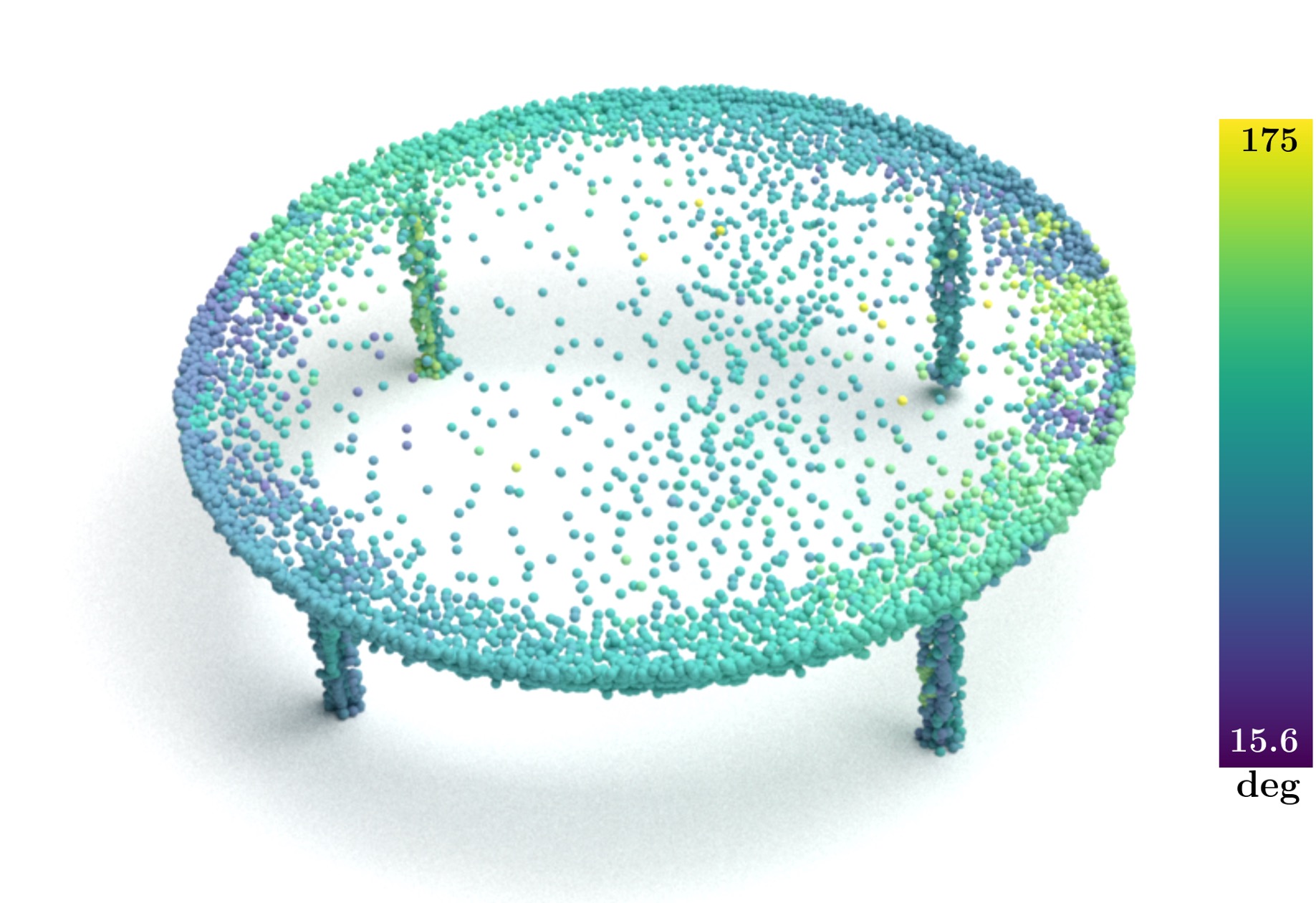
(c) Rotation

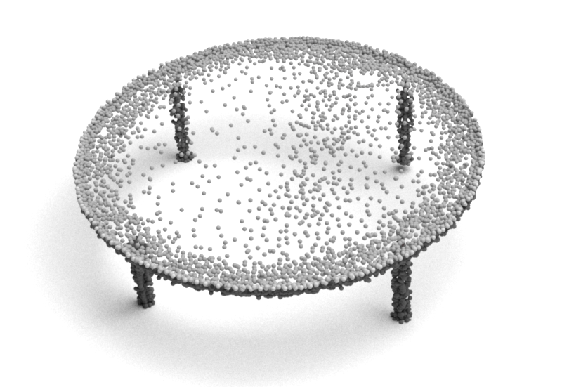
(d) RGB from SH

Figure 4: Splats Centroid Colorized Based on Individual Gaussian Parameter Values. The visualization reveals the complexity of the parameter distribution with respect to spatial dimensions.

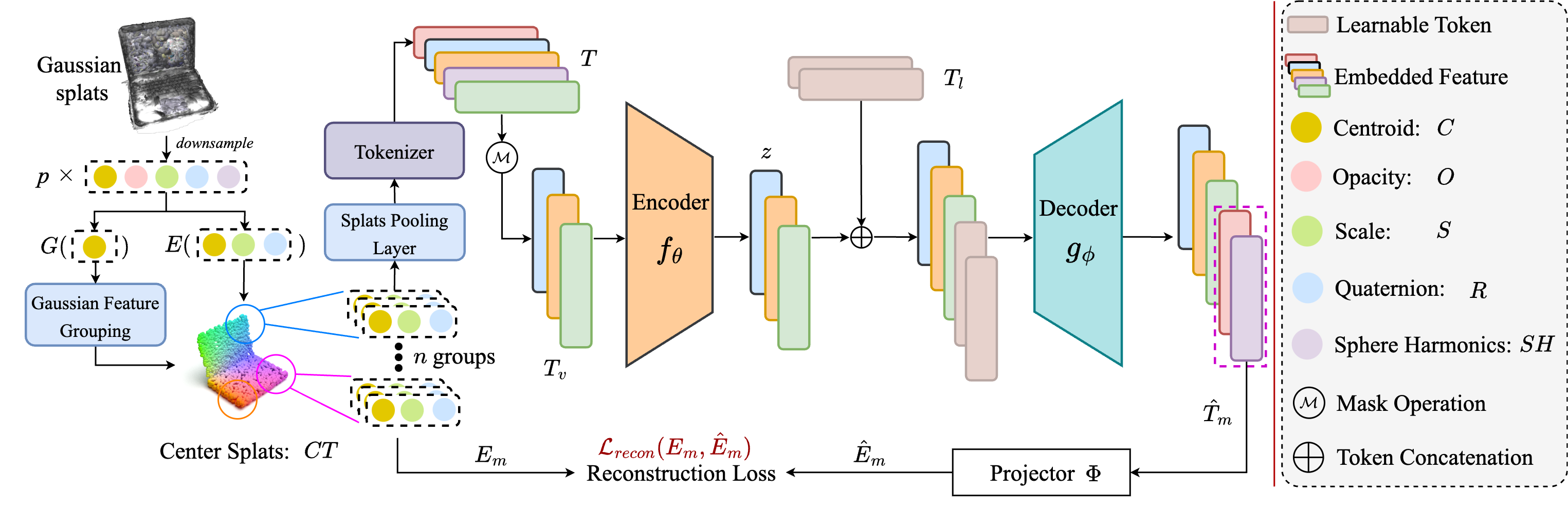
Figure 5: Gaussian-MAE Framework. Given the downsampled Gaussian splats, parameters for the grouping feature $G(\cdot)$ and embedding feature $E(\cdot)$ are first selected. $G(\cdot)$ is used to split the splats into $n$ groups, while $E(\cdot)$ serves as the reconstruction target in the MAE. After the splats pooling layer, the grouped splats are tokenized into group tokens $T$, which are then masked and the visible $T_{v}$ is passed into the encoder $f_{\theta}$ to obtain latent $z$. Following the concatenation of $z$ and the learnable tokens $T_{l}$, the decoder $g_{\theta}$ then recovers the masked tokens $\hat{T}_{m}$, which are projected to obtain the embedding components $\hat{E}_{m}$ for calculating the reconstruction loss $\mathcal{L}_{\textit{recon}}$. As an example, we use $G(C)$ for grouping and $E(C,S,R)$ for embedding, other inputs follow the same process.

Input: Object with $N$ Gaussian splats $X=[C,O,S,R,SH]\in\mathbb{R}^{N\times 59}$

Output: Reconstructed embedding feature $\hat{E}_{m}$ for masked regions

1. Randomly downsample to $p$ Gaussian splats: $X^{\prime}\in\mathbb{R}^{p\times 59}$.

2. Select parameters for the grouping feature $G(\cdot)$ and embedding feature $E(\cdot)$.

3. Compute $n$ center splats from the grouping feature:

   $$CT=\operatorname{FPS}(G),\quad CT\in\mathbb{R}^{n\times f_{G}}.$$

4. Find $k$ neighboring splats and obtain their embedding features:

   $$E_{\text{group}}=\operatorname{KNN}(E;G,CT),\quad E_{\text{group}}\in\mathbb{R}^{n\times k\times f_{E}}.$$

5. Forward the embedding features to the tokenizer to obtain tokens:

   $$T=\operatorname{Tokenizer}(E_{\text{group}}),\quad T\in\mathbb{R}^{n\times D}.$$

6. Masking with a ratio $r$, resulting in visible tokens $T_{v}\in\mathbb{R}^{(1-r)n\times D}$ , masked tokens $T_{m}\in\mathbb{R}^{rn\times D}$. and masked embedding feature $E_{m}$.

7. Obtain the latent $z$ from the encoder: $z=f_{\theta}(T_{v})$.

8. Concatenate $z$ with learnable token $T_{l}$ and then pass to the decoder $g_{\phi}(\cdot)$ to get the recovered masked token $\hat{T}_{m}=g_{\phi}(z\oplus T_{l})$

9. Projector $\Phi$ output the recovered embedding feature $\hat{E}_{m}=\Phi(\hat{T}_{m})$

10. Minimizing the reconstruction loss $\mathcal{L}_{\text{recon}}$:

    $$\min_{\theta,\phi}\underset{\begin{subarray}{c}E\sim\mathcal{\tau}\end{subarray}}{\mathbb{E}}\left[\mathcal{L}_{\text{recon}}\left(E_{m},\hat{E}_{m}\right)\right].$$

Algorithm 1 Gaussian-MAE

3 ShapeSplat Dataset Generation

Since the datasets we choose are in CAD format, we first need to render 2D images at chosen poses to train Gaussian splats. To address the limitations of the original 3DGS [22], which often results in high redundancy [29], we incorporate important-score based pruning [12].

Model Rendering. We adapt the code from [32] to render CAD models in Blender. Each model is rendered from 72 uniformly spaced views, with an image resolution of 400$\times$400 to balance quality and rendering time. A white background is used for clear object distinction, and problematic CAD models are filtered out. Fig. 2 shows our qualitative rendering results.

3DGS Training. After obtaining the image-pose pairs, we initialize the Gaussian centroids using a point cloud of 5K points uniformly sampled from mesh surfaces, following similar practice as in ShapeNet[3] and ModelNet[56]. To reduce the scale artifacts, we employ the regularization term from [64] to penalize large scales. The training process takes approximately 15 minutes per scene over 30,000 iterations. The total time required is detailed in Tab. 1.

Gaussian Pruning. Following the approach in [12], the importance score is calculated based on the contribution of each Gaussian splat to the rendered pixels, taking into account factors such as scale, rotation, and opacity. We prune 60 $\%$ of the Gaussians at iterations 16k and 24k. To avoid artifacts due to pruning, we incorporate pruning during the training process rather than as a post-processing step, ensuring necessary densification occurs throughout training. The final number of Gaussians is reported in Tab. 1.

Dataset Evaluation. Tab. 1 details the statistics of ShapeSplat, including object and category number, training time, number of Gaussians and the average PSNR (peak signal-to-noise ratio) of the renderings used for training. Note that ShapeNet-Part is a subset of ShapeNet-Core, and we report its training time for completeness. The average number of Gaussians exceeds 20K, notably higher than the input with 8K points in the point cloud baseline [36]. Furthermore, we compute the Jensen–Shannon Divergence (JSD) and Maximum Mean Discrepancy (MMD) [70] metrics between the trained Gaussian centroids and the initializing point cloud. These metrics are computed using 50x50 bins and averaged across three views, mapped onto the x, y, and z planes. Despite being initialized from point cloud, the distribution of Gaussian splat centroids differs substantially. The visual differences in distribution are presented in Fig. 3.

4 Gaussian-MAE

Preliminary: 3D Gaussian Splatting. 3DGS parameterizes the scene space with a set of Gaussian primitives $\{X_{i}\}_{i=1}^{N}$, stacking the parameters together,

$$X=[C,O,S,R,SH]\in\mathbb{R}^{N\times 59},$$ (1)

with centroid $C\in\mathbb{R}^{N\times 3}$, opacity $O\in\mathbb{R}^{N\times 1}$, scale $S\in\mathbb{R}^{N\times 3}$, quaternion vector $R\in\mathbb{R}^{N\times 4}$ and sphere harmonics $SH\in\mathbb{R}^{N\times 48}$. We refer to them as Gaussian features or Gaussian parameters. Each Gaussian can be seen as softly representing an area of 3D space with its opacity. A point $q$ in scene space is influenced by a Gaussian $X_{i}$ according to the Gaussian distribution value weighted by its opacity:

$$f_{i}(q)=O_{i}\exp\left(-\frac{1}{2}(q-C_{i})^{T}\Sigma_{i}^{-1}(q-C{i})\right),$$ (2)

where the covariance matrix $\Sigma_{i}$ can be formulated as $\Sigma_{i}=R_{i}S_{i}S_{i}^{T}R_{i}^{T}$.

As the name ”splatting” suggests, the influence function $f$ can be cast onto a 2D image plane for every Gaussian. The rendered color of a pixel is the weighted sum over the colors $c$ in its influencing Gaussians set $\mathcal{S}$, calculated by the alpha-blending equation using the sorted front-to-back order:

$$c_{\text{pixel}}=\sum_{i\in\mathcal{S}}c_{i}f^{\textrm{2D}}_{i}\prod_{j=1}^{i-1}(1-f^{\textrm{2D}}_{j})\enspace.$$ (3)

Through differentiable rasterization, the rendering loss is back-propagated to the trainable Gaussian parameters.

4.1 Gaussian MAE Framework

Fig. 5 illustrates the pipeline of Gaussian-MAE. We report detailed algorithm in Algorithm 1. We define two key features: embedding feature $E$ ($E\subseteq X^{\prime}$ with $E\in\mathbb{R}^{p\times f_{E}}$), a subset of $X^{\prime}$ selected as input to the tokenizer, which is then the reconstruction target, its dimension $f_{E}$ depends on the chosen parameters; and grouping feature $G$ ($G\subseteq X^{\prime}$ with $G\in\mathbb{R}^{p\times f_{G}}$), another subset of $X^{\prime}$ used to compute distances during the grouping process and its dimension $f_{G}$ depends on the chosen parameters. We use centroid grouping $G(C)$ for experiments in Tabs. 2, 3 and 4. Multiple Conv1d projectors $\Phi$ are used for different gaussian parameters and for reconstruction loss $\mathcal{L}_{recon}$ we employ the Chamfer-Distance [11] for centroid and $\mathcal{L}1$ loss for other parameters.

4.2 Gaussian Feature Grouping

Building on Algorithm 1, we propose considering more than centroid during grouping. The reasons for separating grouping and embedding are twofold: firstly, sampling only in centroid space assumes similar correlation between all Gaussian parameters and its center coordinate, which is not the case. As shown in Fig. 4, Gaussian splats with varying opacity and scale can blend together on the surface. Secondly, using additional Gaussian features for grouping allows for the clustering of splats that are not only spatially close but also similar in other attributes. To balance the grouping across gaussian parameters, we recenter all parameters (excluding quaternions) to zero mean and map them to the unit sphere in their respective dimensions. To avoid the complexity of grouping with high-dimensional feature, we select only the $SH$ base $\in\mathbb{R}^{p\times 3}$ for grouping.

4.3 Splats Pooling Layer

Gaussian feature grouping effectively cluster Gaussians into groups by similarity. To further balance the contribution of each parameter, we propose a learned temperature-scaled splats pooling layer customed to Gaussian parameters, aiming to efficiently aggregate information from the embedded feature of the potential neighbors.

Let $B$ denote the batch size, $n$ the number of groups, $P$ the number of potential neighbors per group, $k$ the desired number of nearest neighbors, and $D$ the intermediate embedding dimension. For each center splat, $P$ neighbors are first selected by using KNN on centroids. Then, we apply Conv1d layers to obtain embedding $F$, where $F\in\mathbb{R}^{B\times n\times P\times D}$. For each group in the batch, the query item $y_{b,n}$ is obtained by applying max pooling to $F$ across the dimension $P$. We then compute the pairwise distances between the query item $y_{b,n}$ and potential neighbors as $d_{b,n,p}=\|y_{b,n}-F_{b,n,p}\|^{2}$ for $p\in[1,P]$.

To introduce learnable temperature, we define $\gamma\in\mathbb{R}^{k}$ and $\beta\in\mathbb{R}^{k}$, respectively. The temperatures are computed as $t=\exp(\gamma)+\beta$. Once the softmax weights are calculated by applying a temperature-scaled softmax to the pairwise distances, the resulting weight tensor is $W\in\mathbb{R}^{B\times n\times k\times P}$. These weights are used for feature aggregation, producing the aggregated tensor $Z\in\mathbb{R}^{B\times n\times k\times D}$, where $Z_{b,n,k,d}=\sum_{p=1}^{P}W_{b,n,k,p}\cdot F_{b,n,p,d}$. $Z$ is then served as the input to derive the token for the splats group.

Per-dimension temperature here can depend on the query item, enabling the model to learn when it is beneficial to average more uniformly across the embedding space with high temperature and with low temperature when it should focus on some distinct neighbor embeddings. This is especially needed as Gaussian attributes can exhibit highly uneven distribution as shown in Fig. 4.

5 Experiments

In this section, we extensively present the pretraining results, finetuning performance, generalization experiments, effect of Gaussian space grouping and splats pooling layer, as well as an ablation study. Please refer to our supplement for implementation details.

5.1 Pretraining Results

We conduct extensive pretraining experiments with the proposed Gaussian-MAE method, demonstrating that Gaussian parameters can be successfully reconstructed. Detailed reconstruction analysis is reported in Fig. 6 and qualitative results are included in the supplement. Align with Sec. 4.2 we use $E(\cdot)$ and $G(\cdot)$ for gaussian parameters for embedding and grouping. To distinguish different models in self-supervised learning, we use an * to indicate models pretrained on Gaussians and tested on point clouds, $\dagger$ for models pretrained and fine-tuned both on point clouds. Unless otherwise specified, we default to downsampling to 1024 Gaussians and using a mask ratio of 0.6 in our experiments.

Method	ModelNet10	ModelNet40
Supervised Learning Only
PointNet [39]	$\times$	89.2
PointNet++ [40]	$\times$	91.9
PTv1 [67]	$\times$	90.6
PTv2 [55]	$\times$	91.6
with Standard ViTs Self-Supervised Learning (Full)
Point-BERT$\dagger$ [63]	94.82	93.20
Point-MAE$\dagger$ [37]	94.93	93.20
Gaussian-MAE; $E(C)$	93.72	91.77
Gaussian-MAE; $E(C,O)$	93.83	91.78
Gaussian-MAE; $E(C,SH)$	93.83	92.41
Gaussian-MAE; $E(C,S,R)$	94.27	93.19
Gaussian-MAE; $E(O,C,S,R)$	95.48	92.42
Gaussian-MAE; $E(All)$	95.37	93.35
with Standard ViTs Self-Supervised Learning (MLP-Linear)
Point-BERT$\dagger$ [63]	93.06	90.56
Point-MAE$\dagger$ [37]	93.17	90.24
Gaussian-MAE; $E(C)$	92.73	87.84
Gaussian-MAE; $E(C,O)$	91.30	87.43
Gaussian-MAE; $E(C,SH)$	91.19	86.38
Gaussian-MAE; $E(C,S,R)$	93.28	88.73
Gaussian-MAE; $E(O,C,S,R)$	93.72	88.93
Gaussian-MAE; $E(All)$	93.83	90.64
with Standard ViTs Self-Supervised Learning (MLP-3)
Point-BERT$\dagger$ [63]	94.27	91.82
Point-MAE$\dagger$ [37]	93.61	92.63
Gaussian-MAE; $E(C)$	92.84	90.06
Gaussian-MAE; $E(C,O)$	93.39	89.86
Gaussian-MAE; $E(C,SH)$	93.39	90.72
Gaussian-MAE; $E(C,S,R)$	94.16	90.15
Gaussian-MAE; $E(O,C,S,R)$	93.72	91.29
Gaussian-MAE; $E(All)$	95.26	92.74

Table 2: Classification Accuracy on ModelNet (overall accuracy $\uparrow$ [%]). Best results are highlighted as first, second. $\dagger$ denotes model pretrained and finetuned both on point clouds. Ours with all inputs as embedding feature $E$ yields the best accuracy.

Method	ModelNet40	OBJ_BG	OBJ_ONLY	PB_T50_RS
Supervised Learning Only
PointNet [39]	89.2	73.3	79.2	68.0
PointNet++ [40]	91.9	82.3	84.3	77.9
DGCNN [53]	92.9	82.8	86.2	78.1
PointCNN [25]	92.5	86.1	85.5	78.5
with Standard ViTs Self-Supervised Learning (Full)
Point-MAE$\dagger$ [36]	93.20	90.02	88.29	85.18
Gaussian-MAE*; $E(C)$	92.78	87.61	88.64	84.98
with Standard ViTs Self-Supervised Learning (MLP-Linear)
Point-MAE$\dagger$ [36]	90.24	82.58	83.52	73.08
Gaussian-MAE*;$E(C)$	88.49	70.74	72.63	66.55
with Standard ViTs Self-Supervised Learning (MLP-3)
Point-MAE$\dagger$ [37]	92.63	84.29	85.24	77.34
Gaussian-MAE*; $E(C)$	90.36	81.93	85.37	75.02

Table 3: Generalization Experiments on ModelNet and ScanObjectNN (overall accuracy $\uparrow$ [%]). * indicates models pretrained on Gaussians and tested on point clouds. Despite being pretrained on Gaussian splats, Gaussian-MAE achieves reasonable accuracy on point clouds, even surpassing the dedicated point cloud baseline in OBJ_ONLY accuracy on ScanObjectNN.

5.2 Classification Experiments

To assess the efficacy of the pretrained model, we gauged its performance under three kinds of transfer protocols like [8, 41, 45] for classification tasks during finetuning, i.e., (a) Full: finetuning pretrained models by updating all backbone and classification heads. (b) MLP-Linear: The classification head is a single-layer linear MLP, and we only update these head parameters during finetuning. (c) MLP-3: The classification head is a three-layer non-linear MLP (i.e., the same as the one used in FULL), and we only update these head parameters during finetuning.

We report classification performance on ModelNet10 and ModelNet 40 datasets in Tab. 2. Note that here we use $G(C)$ for grouping and analyzing how different attributes contribute to the classification tasks. Compared to the supervised-only method, our proposed Gaussian-MAE effectively learns shape priors from unlabeled data. Even when using only the Gaussian centroids, our results surpass those of the supervised-only methods. However, we observe that when using only the center positions of the Gaussians, our results are inferior to the unsupervised baseline, Point-MAE, on point clouds. This may be due to the uneven distribution of the Gaussians. Notably, when we use other Gaussian parameters, our performance improves significantly by $0.55\%$. Each component contributes positively to the results, with the scale and rotation components providing the greatest benefit to classification. Furthermore, the performance increase over the baseline becomes even larger when using linear ($0.66\%$) and MLP-3 ($1.65\%$) probing, suggesting that the pretrained features learned by our approach are stronger and more robust.

5.3 Segmentation Experiments

Following the same setting as point cloud pretraining methods like Point-Bert [63], Point-MAE [36], we use the pretrained weight from ShapeNet and finetine on ShapeNet-Part for part segmentation task. From the results reported in Tab. 4, we observed that employing only Gaussian centroid resulted in higher class mIoU compared to Point-MAE, indicating that pretraining on Gaussian centroids offers greater benefits for segmentation. This aligns with our previous findings, as Gaussian distributions, concentrated at boundaries, capture crucial semantic variations. Unlike classification, utilizing opacity, scale, and rotation improves segmentation results, while adding spherical harmonics (SH) negatively impacts performance.

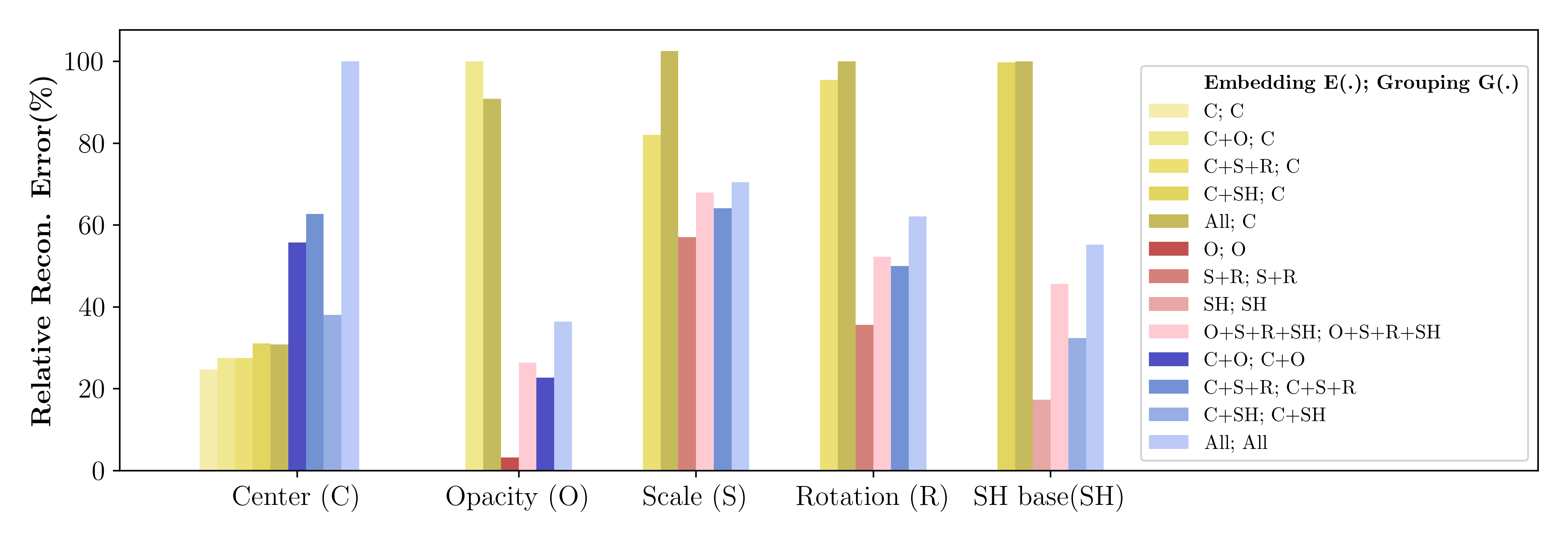
Figure 6: Per-attribute Reconstruction of Different Grouping Method. Relative reconstruction error is reported for each Gaussian parameter using different grouping feature $G$ represented by three different color shades, namely centroid grouping , feature grouping without centroid, and feature grouping with centroid. We observe that better overall reconstruction lead to better performance, cf. Fig. 7.

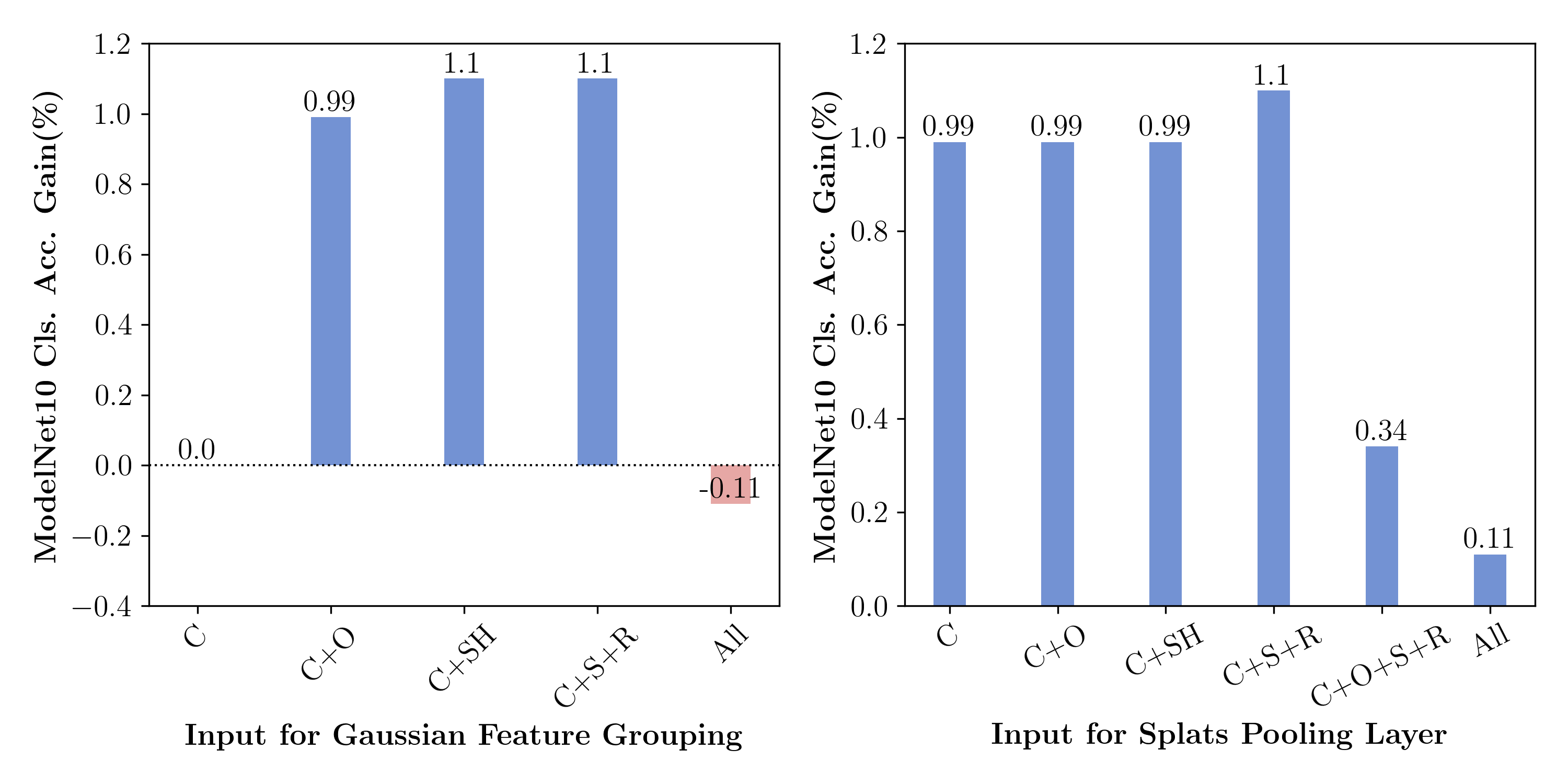
Figure 7: Ablation on Gaussian Feature Grouping and Splats Pooling Layer. Classification accuracy on ModelNet10 significantly improves with the inclusion of both Gaussian feature grouping and splats pooling layer, across different embedding features.

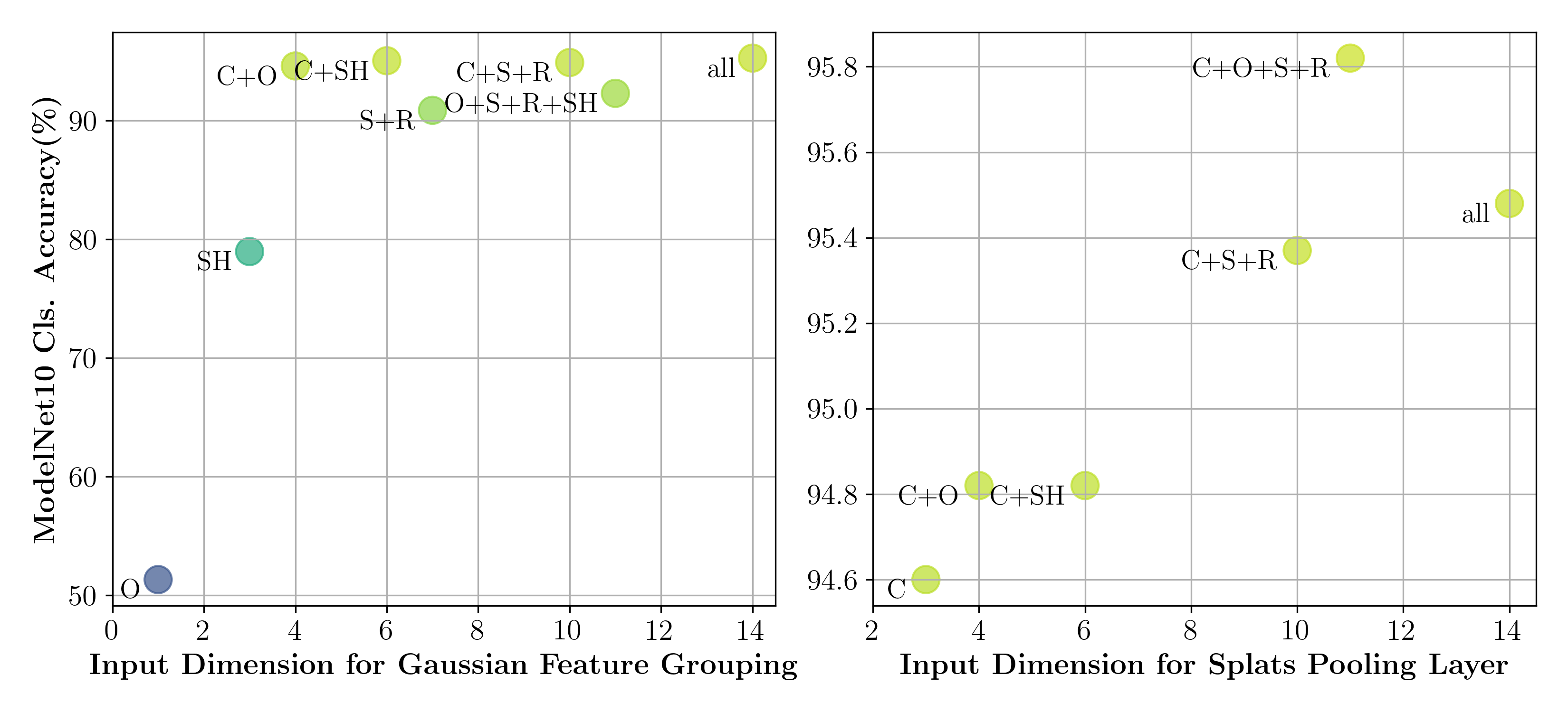
Figure 8: Effect of Input Dimension on Gaussian Feature Grouping and Splats Pooling Layer. Higher input dimensions consistently improve classification accuracy with both modules.

Method	mIoUC (%) $\uparrow$	mIoUI (%) $\uparrow$
Supervised Representation Learning
PointNet [39]	80.4	83.7
PointNet++ [40]	81.9	85.1
Transformer [52]	83.4	85.1
PTv1 [67]	83.7	86.6
with Self-Supervised Representation Learning
Point-BERT$\dagger$ [63]	84.1	85.6
Point-MAE$\dagger$ [37]	84.2	86.1
Gaussian-MAE*; $E(C)$	84.6	86.1
Gaussian-MAE; $E(C)$	84.4	85.8
Gaussian-MAE; $E(C,O)$	84.6	86.1
Gaussian-MAE; $E(C,SH)$	84.0	85.8
Gaussian-MAE; $E(C,S,R)$	84.4	86.0
Gaussian-MAE; $E(C,O,S,R)$	84.2	85.8
Gaussian-MAE; $E(C,All)$	84.4	86.0

Table 4: Part Segmentation on ShapeNet-Part. * indicates models pretrained on Gaussians and tested on point clouds. The class mIoU (mIoU_C) and the instance mIoU (mIoU_I) are reported. Gaussian-MAE yields $0.4\%$ gain in mIoU_C.

5.4 Generalization to Point Clouds

We report results of employing only the Gaussian centroids for pretraining followed by finetuning on point clouds in Tab. 3. Note that we tested on the point cloud data of ModelNet40 and ScanObjectNN. From the results, we can see that when joint training the encoder, the Gaussian-MAE pretraining on Gaussian centroids yields finetuning results close to Point-MAE pretraining on point clouds, and even outperforms the baseline in the Object-only results. However, when freezing the encoder and only training the decoder, the significant difference between the centroid distribution leads to a performance drop, and this gap becomes larger when using a Linear Classification head.

In the segmentation task reported in Tab. 4, we were pleasantly surprised to find that the model pretrained on Gaussian centroids outperformed the point cloud baseline. This suggests that the encoder learned features from the Gaussian data that are more beneficial for segmentation.

5.5 Grouping Feature Grouping Analysis

Effectiveness of Grouping Feature Grouping and Splats Pooling Layer. We first evaluate the effect of grouping on multiple Gaussian parameters for ModelNet10 classification in Fig. 7. Compared to the baseline which groups only by Gaussian center, adding additional parameters individually leads to up to $1.1\%$ increase in classification accuracy. The same accuracy boost also results from the splats pooling layer, which uses the center for grouping but learns to combine multiple patterns for aggregating features from the group. For both methods, including all Gaussian parameters yields diminishing gains, as the baseline encodes stronger features from the parameter space.

Reconstruction Analysis on Grouping Feature Grouping. Fig. 6 reports the relative reconstruction error of each Gaussian parameter with different grouping and embedding input. First we observe that each feature achieves the lowest reconstruction error when it is both embedded and grouped exclusively. Additionally grouping and embedding with other feature make negative impact on centroid reconstruction, while opacity, scale and rotation affect more than SH as shown in the error bars for center. This observation intuitively aligns with Fig. 4, as most colors in ShapeSplat are uniform. We also observe that when grouped with centroid, each parameter has the highest reconstruction error, as indicated by the light green bars of opacity, scale, rotation and SH. As shown by the rightmost light blue bars, when all the attributes are taken into account when grouping, and embedded, the reconstruction errors are large and affect unevenly for different parameter, which we hypothesise resulting from imbalance weighting of each feature. These observations highlight that Gaussian parameters are complexly distributed with respect to spatial dimensions. Furthermore, we conclude from Figs. 7 and 6 that a smaller overall reconstruction error on the target embedding feature enhances performance in classification.

Input Dimension Ablation for Parameter Space Grouping and Splats Pooling Layer. Fig. 8 ablates the total input dimension for Gaussian feature grouping and splats pooling layer with respect to the absolute classification accuracy on ModelNet10. We observe that for Gaussian feature grouping, more dimensions consistently correspond to higher accuracy, whereas for splats pooling layer, it’s generally the case. We obtain the highest accuracy of $95.82\%$ among our experiments using splats pooling layer with the input of center, opacity, scale, and rotation.

5.6 Further Ablation Study

Method	ModelNet10	ModelNet40	ShapeNet-Part
splats input number ablation (Full)
1024	95.37	93.35	84.4
2048	93.29	92.29	84.4
4096	94.82	93.02	84.8
8192	95.26	93.05	84.5
mask ratio ablation (Full)
mask ratio=0.2	95.48	91.73	84.6
mask ratio=0.4	96.03	91.89	84.7
mask ratio=0.6	95.37	93.35	84.4
mask ratio=0.8	95.81	92.46	83.0

Table 5: Ablation on Number of Splats and Mask Ratio.

Ablation on Gaussian Splats Number for Finetuning. Tab. 5 ablates the effect of the number of splats used during finetuning. For the classification task, the best performance occurs when the number of input splats matches that used in pretraining (1024 in this case), likely due to consistent aggregation patterns for patch embeddings. Accuracy improves again as the number of input splats increases further. For segmentation, the mIoU_C generally improves with a higher number of input splats.

Ablation on Mask Ratio in Pretraining. Tab. 5 reports the finetuning performance using the pretrained model with different mask ratios. The results show that as the mask ratio increases initially, both classification and segmentation performance improve, credited to the stronger representation learned by the MAE. As the mask ratio approaches 1, the pretraining target gets much more challenging, which in turn hinders the performance in downstream tasks.

6 Limitation

Compared to original number of Gaussian Splats shown in Tab. 1, we significantly downsample them before pretraining, which mimics the processing of point clouds. However, this is sub-optimal, as the downsampled splats lose important appearance and geometry details, which then hinder the learned representation. An efficient mechanism to directly operate on the original splats is an interesting direction for future work.

7 Conclusion

We present ShapeSplat dataset which enables the masked pretraining directly on 3DGS parameters. Experiments show that naively treating Gaussian centroids as point clouds does not perform well in downstream tasks. In contrast, our Gaussian-MAE method excels by effectively aggregating features using Gaussian feature grouping and splats pooling layer. We hope this work opens a new avenue for self-supervised 3D representation learning.

Appendix

A Nomenclature

References

- Bortolon et al. [2024] Matteo Bortolon, Theodore Tsesmelis, Stuart James, Fabio Poiesi, and Alessio Del Bue. 6dgs: 6d pose estimation from a single image and a 3d gaussian splatting model. In ECCV, 2024.
- Brown et al. [2020] Tom Brown, Benjamin Mann, Nick Ryder, Melanie Subbiah, Jared D Kaplan, Prafulla Dhariwal, Arvind Neelakantan, Pranav Shyam, Girish Sastry, Amanda Askell, et al. Language models are few-shot learners. Advances in neural information processing systems, 33:1877–1901, 2020.
- Chang et al. [2015] Angel X. Chang, Thomas Funkhouser, Leonidas Guibas, Pat Hanrahan, Qixing Huang, Zimo Li, Silvio Savarese, Manolis Savva, Shuran Song, Hao Su, Jianxiong Xiao, Li Yi, and Fisher Yu. ShapeNet: An Information-Rich 3D Model Repository. Technical Report arXiv:1512.03012 [cs.GR], Stanford University — Princeton University — Toyota Technological Institute at Chicago, 2015.
- Collins et al. [2022] Jasmine Collins, Shubham Goel, Kenan Deng, Achleshwar Luthra, Leon Xu, Erhan Gundogdu, Xi Zhang, Tomas F Yago Vicente, Thomas Dideriksen, Himanshu Arora, et al. Abo: Dataset and benchmarks for real-world 3d object understanding. In Proceedings of the IEEE/CVF conference on computer vision and pattern recognition, pages 21126–21136, 2022.
- Deitke et al. [2023] Matt Deitke, Dustin Schwenk, Jordi Salvador, Luca Weihs, Oscar Michel, Eli VanderBilt, Ludwig Schmidt, Kiana Ehsani, Aniruddha Kembhavi, and Ali Farhadi. Objaverse: A universe of annotated 3d objects. In Proceedings of the IEEE/CVF Conference on Computer Vision and Pattern Recognition, pages 13142–13153, 2023.
- Deitke et al. [2024] Matt Deitke, Ruoshi Liu, Matthew Wallingford, Huong Ngo, Oscar Michel, Aditya Kusupati, Alan Fan, Christian Laforte, Vikram Voleti, Samir Yitzhak Gadre, et al. Objaverse-xl: A universe of 10m+ 3d objects. Advances in Neural Information Processing Systems, 36, 2024.
- Devlin et al. [2018] Jacob Devlin, Ming-Wei Chang, Kenton Lee, and Kristina Toutanova. Bert: Pre-training of deep bidirectional transformers for language understanding. arXiv preprint arXiv:1810.04805, 2018.
- Dong et al. [2022] Runpei Dong, Zekun Qi, Linfeng Zhang, Junbo Zhang, Jianjian Sun, Zheng Ge, Li Yi, and Kaisheng Ma. Autoencoders as cross-modal teachers: Can pretrained 2d image transformers help 3d representation learning? In The Eleventh International Conference on Learning Representations, 2022.
- Dosovitskiy et al. [2020] Alexey Dosovitskiy, Lucas Beyer, Alexander Kolesnikov, Dirk Weissenborn, Xiaohua Zhai, Thomas Unterthiner, Mostafa Dehghani, Matthias Minderer, Georg Heigold, Sylvain Gelly, et al. An image is worth 16x16 words: Transformers for image recognition at scale. In International Conference on Learning Representations (ICLR), 2020.
- Downs et al. [2022] Laura Downs, Anthony Francis, Nate Koenig, Brandon Kinman, Ryan Hickman, Krista Reymann, Thomas B McHugh, and Vincent Vanhoucke. Google scanned objects: A high-quality dataset of 3d scanned household items. In 2022 International Conference on Robotics and Automation (ICRA), pages 2553–2560. IEEE, 2022.
- Fan et al. [2017] Haoqiang Fan, Hao Su, and Leonidas J Guibas. A point set generation network for 3d object reconstruction from a single image. In Proceedings of the IEEE conference on computer vision and pattern recognition, pages 605–613, 2017.
- Fan et al. [2023] Zhiwen Fan, Kevin Wang, Kairun Wen, Zehao Zhu, Dejia Xu, and Zhangyang Wang. Lightgaussian: Unbounded 3d gaussian compression with 15x reduction and 200+ fps. arXiv preprint arXiv:2311.17245, 2023.
- Fu et al. [2020] Huan Fu, Rongfei Jia, Lin Gao, Mingming Gong, Binqiang Zhao, Steve Maybank, and Dacheng Tao. 3d-future: 3d furniture shape with texture, 2020.
- Gao et al. [2024] Quankai Gao, Qiangeng Xu, Zhe Cao, Ben Mildenhall, Wenchao Ma, Le Chen, Danhang Tang, and Ulrich Neumann. Gaussianflow: Splatting gaussian dynamics for 4d content creation. arXiv preprint arXiv:2403.12365, 2024.
- Grill et al. [2020] Jean-Bastien Grill, Florian Strub, Florent Altché, Corentin Tallec, Pierre Richemond, Elena Buchatskaya, Carl Doersch, Bernardo Avila Pires, Zhaohan Guo, Mohammad Gheshlaghi Azar, et al. Bootstrap your own latent-a new approach to self-supervised learning. Advances in neural information processing systems, 33:21271–21284, 2020.
- Guédon and Lepetit [2024] Antoine Guédon and Vincent Lepetit. Sugar: Surface-aligned gaussian splatting for efficient 3d mesh reconstruction and high-quality mesh rendering. In Proceedings of the IEEE/CVF Conference on Computer Vision and Pattern Recognition, pages 5354–5363, 2024.
- He et al. [2022] Kaiming He, Xinlei Chen, Saining Xie, Yanghao Li, Piotr Dollár, and Ross Girshick. Masked autoencoders are scalable vision learners. In Proceedings of the IEEE/CVF conference on computer vision and pattern recognition, pages 16000–16009, 2022.
- Hess et al. [2023] Georg Hess, Johan Jaxing, Elias Svensson, David Hagerman, Christoffer Petersson, and Lennart Svensson. Masked autoencoder for self-supervised pre-training on lidar point clouds. In Proceedings of the IEEE/CVF winter conference on applications of computer vision, pages 350–359, 2023.
- Huang et al. [2024] Binbin Huang, Zehao Yu, Anpei Chen, Andreas Geiger, and Shenghua Gao. 2d gaussian splatting for geometrically accurate radiance fields. In ACM SIGGRAPH 2024 Conference Papers, pages 1–11, 2024.
- Irshad et al. [2024a] Muhammad Zubair Irshad, Sergey Zakahrov, Vitor Guizilini, Adrien Gaidon, Zsolt Kira, and Rares Ambrus. Nerf-mae: Masked autoencoders for self supervised 3d representation learning for neural radiance fields. arXiv preprint arXiv:2404.01300, 2024a.
- Irshad et al. [2024b] Muhammad Zubair Irshad, Sergey Zakharov, Vitor Guizilini, Adrien Gaidon, Zsolt Kira, and Rares Ambrus. Nerf-mae: Masked autoencoders for self-supervised 3d representation learning for neural radiance fields. 2024b.
- Kerbl et al. [2023] Bernhard Kerbl, Georgios Kopanas, Thomas Leimkühler, and George Drettakis. 3d gaussian splatting for real-time radiance field rendering. ACM Trans. Graph., 42(4):139–1, 2023.
- Lei et al. [2024a] Jiahui Lei, Yufu Wang, Georgios Pavlakos, Lingjie Liu, and Kostas Daniilidis. Gart: Gaussian articulated template models. In Proceedings of the IEEE/CVF Conference on Computer Vision and Pattern Recognition, pages 19876–19887, 2024a.
- Lei et al. [2024b] Jiahui Lei, Yijia Weng, Adam Harley, Leonidas Guibas, and Kostas Daniilidis. Mosca: Dynamic gaussian fusion from casual videos via 4d motion scaffolds. arXiv preprint arXiv:2405.17421, 2024b.
- Li et al. [2018] Yangyan Li, Rui Bu, Mingchao Sun, Wei Wu, Xinhan Di, and Baoquan Chen. Pointcnn: Convolution on x-transformed points. Advances in neural information processing systems, 31, 2018.
- Liang et al. [2022] Yaqian Liang, Shanshan Zhao, Baosheng Yu, Jing Zhang, and Fazhi He. Meshmae: Masked autoencoders for 3d mesh data analysis. In European Conference on Computer Vision, pages 37–54. Springer, 2022.
- Liu et al. [2021] Ze Liu, Yutong Lin, Yue Cao, Han Hu, Yixuan Wei, Zheng Zhang, Stephen Lin, and Baining Guo. Swin transformer: Hierarchical vision transformer using shifted windows. In Proceedings of the IEEE/CVF international conference on computer vision, pages 10012–10022, 2021.
- Liu et al. [2024] Zhiheng Liu, Hao Ouyang, Qiuyu Wang, Ka Leong Cheng, Jie Xiao, Kai Zhu, Nan Xue, Yu Liu, Yujun Shen, and Yang Cao. Infusion: Inpainting 3d gaussians via learning depth completion from diffusion prior. arXiv preprint arXiv:2404.11613, 2024.
- Lu et al. [2024] Tao Lu, Mulin Yu, Linning Xu, Yuanbo Xiangli, Limin Wang, Dahua Lin, and Bo Dai. Scaffold-gs: Structured 3d gaussians for view-adaptive rendering. In Proceedings of the IEEE/CVF Conference on Computer Vision and Pattern Recognition, pages 20654–20664, 2024.
- Luiten et al. [2024] Jonathon Luiten, Georgios Kopanas, Bastian Leibe, and Deva Ramanan. Dynamic 3d gaussians: Tracking by persistent dynamic view synthesis. In 2024 International Conference on 3D Vision (3DV), pages 800–809. IEEE, 2024.
- Ma et al. [2024] Qi Ma, Danda Pani Paudel, Ender Konukoglu, and Luc Van Gool. Implicit-zoo: A large-scale dataset of neural implicit functions for 2d images and 3d scenes. arXiv preprint arXiv:2406.17438, 2024.
- Mildenhall et al. [2020] Ben Mildenhall, Pratul P. Srinivasan, Matthew Tancik, Jonathan T. Barron, Ravi Ramamoorthi, and Ren Ng. Nerf: Representing scenes as neural radiance fields for view synthesis, 2020.
- Morgenstern et al. [2023] Wieland Morgenstern, Florian Barthel, Anna Hilsmann, and Peter Eisert. Compact 3d scene representation via self-organizing gaussian grids. arXiv preprint arXiv:2312.13299, 2023.
- Morrison et al. [2020] Douglas Morrison, Peter Corke, and Jürgen Leitner. Egad! an evolved grasping analysis dataset for diversity and reproducibility in robotic manipulation. IEEE Robotics and Automation Letters, 5(3):4368–4375, 2020.
- Niedermayr et al. [2024] Simon Niedermayr, Josef Stumpfegger, and Rüdiger Westermann. Compressed 3d gaussian splatting for accelerated novel view synthesis. In Proceedings of the IEEE/CVF Conference on Computer Vision and Pattern Recognition, pages 10349–10358, 2024.
- Pang et al. [2022a] Yatian Pang, Wenxiao Wang, Francis EH Tay, Wei Liu, Yonghong Tian, and Li Yuan. Masked autoencoders for point cloud self-supervised learning. In European conference on computer vision, pages 604–621. Springer, 2022a.
- Pang et al. [2022b] Yatian Pang, Wenxiao Wang, Francis E. H. Tay, Wei Liu, Yonghong Tian, and Li Yuan. Masked autoencoders for point cloud self-supervised learning, 2022b.
- Park et al. [2018] Keunhong Park, Konstantinos Rematas, Ali Farhadi, and Steven M Seitz. Photoshape: Photorealistic materials for large-scale shape collections. arXiv preprint arXiv:1809.09761, 2018.
- Qi et al. [2017a] Charles R Qi, Hao Su, Kaichun Mo, and Leonidas J Guibas. Pointnet: Deep learning on point sets for 3d classification and segmentation. In Proceedings of the IEEE conference on computer vision and pattern recognition, pages 652–660, 2017a.
- Qi et al. [2017b] Charles Ruizhongtai Qi, Li Yi, Hao Su, and Leonidas J Guibas. Pointnet++: Deep hierarchical feature learning on point sets in a metric space. Advances in neural information processing systems, 30, 2017b.
- Qi et al. [2023] Zekun Qi, Runpei Dong, Guofan Fan, Zheng Ge, Xiangyu Zhang, Kaisheng Ma, and Li Yi. Contrast with reconstruct: Contrastive 3d representation learning guided by generative pretraining. In International Conference on Machine Learning, pages 28223–28243. PMLR, 2023.
- Qian et al. [2023] Shenhan Qian, Tobias Kirschstein, Liam Schoneveld, Davide Davoli, Simon Giebenhain, and Matthias Nießner. Gaussianavatars: Photorealistic head avatars with rigged 3d gaussians. arXiv preprint arXiv:2312.02069, 2023.
- Qin et al. [2024] Minghan Qin, Wanhua Li, Jiawei Zhou, Haoqian Wang, and Hanspeter Pfister. Langsplat: 3d language gaussian splatting. In Proceedings of the IEEE/CVF Conference on Computer Vision and Pattern Recognition, pages 20051–20060, 2024.
- Ren et al. [2023] Bin Ren, Yahui Liu, Yue Song, Wei Bi, Rita Cucchiara, Nicu Sebe, and Wei Wang. Masked jigsaw puzzle: A versatile position embedding for vision transformers. In Proceedings of the IEEE/CVF Conference on Computer Vision and Pattern Recognition, pages 20382–20391, 2023.
- Ren et al. [2024] Bin Ren, Guofeng Mei, Danda Pani Paudel, Weijie Wang, Yawei Li, Mengyuan Liu, Rita Cucchiara, Luc Van Gool, and Nicu Sebe. Bringing masked autoencoders explicit contrastive properties for point cloud self-supervised learning. arXiv preprint arXiv:2407.05862, 2024.
- Rolfe [2016] Jason Tyler Rolfe. Discrete variational autoencoders. arXiv preprint arXiv:1609.02200, 2016.
- Sandström et al. [2024] Erik Sandström, Keisuke Tateno, Michael Oechsle, Michael Niemeyer, Luc Van Gool, Martin R Oswald, and Federico Tombari. Splat-slam: Globally optimized rgb-only slam with 3d gaussians. arXiv preprint arXiv:2405.16544, 2024.
- Tang et al. [2023] Jiaxiang Tang, Jiawei Ren, Hang Zhou, Ziwei Liu, and Gang Zeng. Dreamgaussian: Generative gaussian splatting for efficient 3d content creation. arXiv preprint arXiv:2309.16653, 2023.
- Tang et al. [2024] Jiaxiang Tang, Zhaoxi Chen, Xiaokang Chen, Tengfei Wang, Gang Zeng, and Ziwei Liu. Lgm: Large multi-view gaussian model for high-resolution 3d content creation. arXiv preprint arXiv:2402.05054, 2024.
- Uy et al. [2019] Mikaela Angelina Uy, Quang-Hieu Pham, Binh-Son Hua, Thanh Nguyen, and Sai-Kit Yeung. Revisiting point cloud classification: A new benchmark dataset and classification model on real-world data. In Proceedings of the IEEE/CVF international conference on computer vision, pages 1588–1597, 2019.
- Van den Herrewegen et al. [2023] Jarne Van den Herrewegen, T Tourwé, et al. Point cloud classification with modelnet40: What is left? In DMLR, Data-centric Machine Learning Research Workshop at the 40 th International Conference on Machine Learning, 2023.
- Vaswani et al. [2023] Ashish Vaswani, Noam Shazeer, Niki Parmar, Jakob Uszkoreit, Llion Jones, Aidan N. Gomez, Lukasz Kaiser, and Illia Polosukhin. Attention is all you need, 2023.
- Wang et al. [2019] Yue Wang, Yongbin Sun, Ziwei Liu, Sanjay E Sarma, Michael M Bronstein, and Justin M Solomon. Dynamic graph cnn for learning on point clouds. Acm Transactions On Graphics (tog), 38(5):1–12, 2019.
- Wu et al. [2023] Tong Wu, Jiarui Zhang, Xiao Fu, Yuxin Wang, Jiawei Ren, Liang Pan, Wayne Wu, Lei Yang, Jiaqi Wang, Chen Qian, et al. Omniobject3d: Large-vocabulary 3d object dataset for realistic perception, reconstruction and generation. In Proceedings of the IEEE/CVF Conference on Computer Vision and Pattern Recognition, pages 803–814, 2023.
- Wu et al. [2022] Xiaoyang Wu, Yixing Lao, Li Jiang, Xihui Liu, and Hengshuang Zhao. Point transformer v2: Grouped vector attention and partition-based pooling, 2022.
- Wu et al. [2015] Zhirong Wu, Shuran Song, Aditya Khosla, Fisher Yu, Linguang Zhang, Xiaoou Tang, and Jianxiong Xiao. 3d shapenets: A deep representation for volumetric shapes. In Proceedings of the IEEE conference on computer vision and pattern recognition, pages 1912–1920, 2015.
- Xie et al. [2024] Tianyi Xie, Zeshun Zong, Yuxing Qiu, Xuan Li, Yutao Feng, Yin Yang, and Chenfanfu Jiang. Physgaussian: Physics-integrated 3d gaussians for generative dynamics. In Proceedings of the IEEE/CVF Conference on Computer Vision and Pattern Recognition, pages 4389–4398, 2024.
- Yang et al. [2023] Yu-Qi Yang, Yu-Xiao Guo, Jian-Yu Xiong, Yang Liu, Hao Pan, Peng-Shuai Wang, Xin Tong, and Baining Guo. Swin3d: A pretrained transformer backbone for 3d indoor scene understanding. arXiv preprint arXiv:2304.06906, 2023.
- Yang et al. [2024] Ziyi Yang, Xinyu Gao, Wen Zhou, Shaohui Jiao, Yuqing Zhang, and Xiaogang Jin. Deformable 3d gaussians for high-fidelity monocular dynamic scene reconstruction. In Proceedings of the IEEE/CVF Conference on Computer Vision and Pattern Recognition, pages 20331–20341, 2024.
- Ye et al. [2023] Mingqiao Ye, Martin Danelljan, Fisher Yu, and Lei Ke. Gaussian grouping: Segment and edit anything in 3d scenes. arXiv preprint arXiv:2312.00732, 2023.
- Yi et al. [2016] Li Yi, Vladimir G Kim, Duygu Ceylan, I-Chao Shen, Mengyan Yan, Hao Su, Cewu Lu, Qixing Huang, Alla Sheffer, and Leonidas Guibas. A scalable active framework for region annotation in 3d shape collections. ACM Transactions on Graphics (ToG), 35(6):1–12, 2016.
- Yi et al. [2024] Taoran Yi, Jiemin Fang, Junjie Wang, Guanjun Wu, Lingxi Xie, Xiaopeng Zhang, Wenyu Liu, Qi Tian, and Xinggang Wang. Gaussiandreamer: Fast generation from text to 3d gaussians by bridging 2d and 3d diffusion models. In Proceedings of the IEEE/CVF Conference on Computer Vision and Pattern Recognition, pages 6796–6807, 2024.
- Yu et al. [2022] Xumin Yu, Lulu Tang, Yongming Rao, Tiejun Huang, Jie Zhou, and Jiwen Lu. Point-bert: Pre-training 3d point cloud transformers with masked point modeling, 2022.
- Yugay et al. [2023] Vladimir Yugay, Yue Li, Theo Gevers, and Martin R Oswald. Gaussian-slam: Photo-realistic dense slam with gaussian splatting. arXiv preprint arXiv:2312.10070, 2023.
- Zhang et al. [2024] Baowen Zhang, Chuan Fang, Rakesh Shrestha, Yixun Liang, Xiaoxiao Long, and Ping Tan. Rade-gs: Rasterizing depth in gaussian splatting. arXiv preprint arXiv:2406.01467, 2024.
- Zhang et al. [2022] Renrui Zhang, Ziyu Guo, Peng Gao, Rongyao Fang, Bin Zhao, Dong Wang, Yu Qiao, and Hongsheng Li. Point-m2ae: multi-scale masked autoencoders for hierarchical point cloud pre-training. Advances in neural information processing systems, 35:27061–27074, 2022.
- Zhao et al. [2021] Hengshuang Zhao, Li Jiang, Jiaya Jia, Philip HS Torr, and Vladlen Koltun. Point transformer. In Proceedings of the IEEE/CVF international conference on computer vision, pages 16259–16268, 2021.
- Zhou and Jacobson [2016] Qingnan Zhou and Alec Jacobson. Thingi10k: A dataset of 10,000 3d-printing models. arXiv preprint arXiv:1605.04797, 2016.
- Zhou et al. [2024] Shijie Zhou, Haoran Chang, Sicheng Jiang, Zhiwen Fan, Zehao Zhu, Dejia Xu, Pradyumna Chari, Suya You, Zhangyang Wang, and Achuta Kadambi. Feature 3dgs: Supercharging 3d gaussian splatting to enable distilled feature fields. In Proceedings of the IEEE/CVF Conference on Computer Vision and Pattern Recognition, pages 21676–21685, 2024.
- Zyrianov et al. [2022] Vlas Zyrianov, Xiyue Zhu, and Shenlong Wang. Learning to generate realistic lidar point clouds, 2022.