On Learning Action Costs from Input Plans

Abstract

Most of the work on learning action models focus on learning the actions’ dynamics from input plans. This allows us to specify the valid plans of a planning task. However, very little work focuses on learning action costs, which in turn allows us to rank the different plans. In this paper we introduce a new problem: that of learning the costs of a set of actions such that a set of input plans are optimal under the resulting planning model. To solve this problem we present $\textsc{lacfip}^{k}$, an algorithm to learn action’s costs from unlabeled input plans. We provide theoretical and empirical results showing how $\textsc{lacfip}^{k}$ can successfully solve this task.

Introduction

Classical planning is the task of choosing and organizing a sequence of deterministic actions such that, when applied in a given initial state, it results in a goal state (Ghallab, Nau, and Traverso 2004). Most planning works assume the actions’ dynamics or domain model, i.e., how actions change the state, are provided as an input and turn the focus to the efficient synthesis of plans. This is a strong assumption in many real-world planning applications, where domain modeling is often a challenging task (Kambhampati 2007). Motivated by the difficulty of crafting action models, several works have tried to automatically learn domain models from input observations (Yang, Wu, and Jiang 2007; Gregory and Lindsay 2016; Arora et al. 2018; Aineto, Celorrio, and Onaindia 2019; Gragera et al. 2023; Garrido 2023). Although they make different assumptions on the type of observations (full or partial plan, access to intermediate states, noisy observations, etc.), most works solely focus on learning the actions’ dynamics but not their associated cost.

In this paper we argue that learning action costs is as important as learning the actions’ dynamics. While actions’ dynamics allow us to determine the validity of traces in a domain model, the actions costs allow us to get the quality of each of these traces, which is needed whenever we want to generate good plans. Moreover, there are many real-world planning applications where the actions’ dynamics are known, but their cost is either unknown and we aim to learn it from scratch; or approximate and we aim to refine it. In both cases we can use data in the form of observed plans to acquire this knowledge.

Consider the case of a navigation tool that suggests routes to drivers. In this domain the actions’ dynamics are clear: cars can move through different roads and taking an action (i.e., taking an exit) will change the car’s position. The navigation tool will typically aim to generate the route with the shortest driving time, i.e., the least costly or optimal plan. To do that, it makes some assumptions about the cost of each action (driving times): for example, being a function of the distance. While this can be a good proxy, it can be further refined by observing the actual plans coming from users of the navigation tool. By observing these plans we cannot only get more accurate driving times, but also understand which routes users prefer and adjust the model accordingly. Financial planning is yet another example where we have access to many plans, actions’ dynamics are known, but properly estimating their cost for different people is crucial and challenging. Pozanco et al. (2023) aim to generate realistic financial plans by maximizing their likelihood. To do that, they assign lower costs to more likely actions, i.e., saving $\$5$ in memberships is less costly than increasing the salary by $\$1,000$. Pozanco et al. mention that these costs can be given or inferred from data but do not provide further details on how to do it. Like in the navigation tool case, here we could gather observed plans on how users are saving and spending money to achieve their financial goals. By doing this, we could more accurately assign costs to each action so as to generate plans that better align with user preferences.

In this paper we introduce a new problem: that of learning the costs of a set of actions such that a set of input plans are optimal under the resulting planning model. We formally prove that this problem does not have a solution for an arbitrary set of input plans, and relax the problem to accept solutions where the number of input plans that are turned optimal is maximized. We also present variations of this problem, where we guarantee input plans are the only optimal plans allowed; or we try to minimally modify an existing cost function instead of learning it from scratch. We then introduce $\textsc{lacfip}^{k}$, a common algorithm to solve these tasks. Empirical results across different planning domains show how $\textsc{lacfip}^{k}$ can be used in practice to learn (or adapt) cost functions from unlabeled input plans.

Preliminaries

A classical planning tasks can be defined as follows:

Definition 1 (strips planning task).

A strips planning task can be defined as a tuple ${\cal P}=\langle F,A,I,G,C\rangle$, where $F$ is a set of fluents, $A$ is a set of actions, $I\subseteq F$ is an initial state, $G\subseteq F$ is a goal state, and $C:A\mapsto\mathbb{N}^{+}_{1}$ is the cost function that associates a cost to each action.

A state $s\subseteq F$ is a set of fluents that are true at a given time. With $\cal S$ we refer to all the possible states defined over $F$. Each action $a\in A$ is described by a set of preconditions $\textsc{pre}(a)$, add effects $\textsc{add}(a)$, delete effects $\textsc{del}(a)$, and cost $c(a)$. An action $a$ is applicable in a state $s$ iff $\textsc{pre}(a)\subseteq~{}s$. We define the result of applying an action in a state as $\gamma(s,a)=(s\setminus\textsc{del}(a))\cup\textsc{add}(a)$.

A sequence of actions $\pi=(a_{1},\ldots,a_{n})$ is applicable in a state $s_{0}$ if there are states $(s_{1}.\ldots,s_{n})$ such that $a_{i}$ is applicable in $s_{i-1}$ and $s_{i}=\gamma(s_{i-1},a_{i})$. The resulting state after applying a sequence of actions is $\Gamma(s,\pi)=s_{n}$, and $c(\pi)=\sum_{i=\{1,\ldots,n\}}c(a_{i})$ denotes the cost of $\pi$. A state $s\in\cal S$ is reachable iff there exists a sequence of actions $\pi$ applicable from $I$ such that $s\subseteq\Gamma(I,\pi)$. With ${\cal S}_{R}\subseteq\cal S$ we refer to the set of all reachable states of the planning task. A sequence of actions is simple if it does not traverse the same state $s\in{\cal S}_{R}$ more than once. A plan $\pi_{i}$ is a subset of a plan $\pi_{j}$ iff the sequence of actions $\pi_{i}=(a_{1},\ldots,a_{n})$ is contained in the sequence of actions that conform $\pi_{j}$. We denote this condition as $\pi_{i}\subset\pi_{j}$.

The solution to a planning task ${\cal P}$ is a plan, i.e., a sequence of actions $\pi$ such that $G\subseteq\Gamma(I,\pi)$. We denote as $\Pi({\cal P})$ the set of all simple solution plans to planning task ${\cal P}$. Also, given a plan $\pi$, we denote its alternatives, i.e., all the other sequence of actions that can solve ${\cal P}$ as $\Pi^{\pi}=\Pi({\cal P})\setminus\pi$.

Definition 2 (Optimal plan).

A plan $\pi$ optimally solves a planning task ${\cal P}$ iff its cost is lower or equal than that of the rest of alternative plans solving ${\cal P}$:

$$c(\pi)\leq c(\pi^{\prime}),\quad\operatorname*{\scalerel*{\forall}{\sum}}_{\pi^{\prime}\in\Pi^{\pi}}$$ (1)

We will use the boolean function $\textsc{is\_optimal}(\pi,{\cal P})$ to evaluate whether $\pi$ optimally solves ${\cal P}$ ($1$) or not ($0$).

Learning Action Costs from Input Plans

We are interested in learning the costs of a set of actions such that the input plans are optimal under the resulting planning model. The underlying motivation is that by aligning the action’s costs to the input plans, the new model will be able to generate new plans that better reflect the observed behavior.

Initially, we assume actions do not have an associated cost a priori. To accommodate this, we extend the potential values that a cost function can have, to include empty values $C:A\mapsto\mathbb{N}^{+}_{1}\cup\{\varnothing\}$. We denote $C=\varnothing$ iff $\forall a\in A,c(a)=\varnothing$. We then formally define a cost function learning task as follows:

Definition 3 (Cost Function Learning Task).

A cost function learning task is a tuple $\textsc{cfl}=\langle{\cal T},{\cal M}\rangle$ where:

• ${\cal T}=({\cal P}_{1},\ldots,{\cal P}_{n})$ is a sequence of planning tasks that share $F$, $A$, and $C=\varnothing$.

• ${\cal M}=(\pi_{1},\ldots,\pi_{n})$ is a corresponding sequence of simple plans that solves ${\cal T}$.

The solution to a cfl task is a common cost function (common across all tasks and plans) $C$.

Let us examine the problem definition. We assume we have access to the full plan $\pi_{i}$ as well as the planning task ${\cal P}_{i}$ that it solves. However, unlike previous works on action’s cost learning (Gregory and Lindsay 2016; Garrido 2023), we do not require to know the total cost of each plan. Moreover, we also assume that all the planning tasks and plans share the same vocabulary, i.e., they have a common set of fluents $F$ and actions $A$. We also assume the common cost function is initially unknown. Finally, we do not make any assumption on the initial and goal state of the input tasks and plans.

The above assumptions are not restrictive and hold in many real-world applications such as the ones described in the Introduction. For example, in the navigation scenario $F$ and $A$ will remain constant as long as the city network (map) does not change, which will only occur when a new road is built. In this domain we will get input plans with different starting points ($I$) and destinations ($G$), which is supported by our problem definition. One could argue that in the navigation scenario it is trivial to annotate each plan with its actual duration. While this might be true, it is clearly not so for other applications where action’s cost capture probabilities or user preferences, such as financial planning.

Going back to Definition 3, we purposely left open the characterization of a cfl solution, only restricting it to be a common cost function $C$ shared by all the input tasks. We did this because we are interested in defining different solution concepts depending on the properties the cost function $C$ should have. In the next subsections we formalize different solutions to cost function learning tasks.

Turning All the Input Plans Optimal

The first objective we turn our attention to is trying to find a common cost function under which all the input plans are optimal. We refer to such solutions as Ideal Cost Functions.

Definition 4 (Ideal Cost Function).

Given a cfl task, we define an ideal cost function icf that solves it as a common cost function $C$ under which all the plans in ${\cal M}$ are optimal. The quality of an ideal cost function is defined as follows:

$$\min\sum_{a\in A}c(a),$$ (2)

$$\text{s.t.}\sum_{i\in{\cal T},{\cal M}}\textsc{is\_optimal}(\pi_{i},{\cal P}_{i}=\langle F,A,I_{i},G_{i},C\rangle)=\lvert{\cal M}\rvert,$$ (3)

An icf is optimal iff no other cost function $C^{\prime}$ yields a lower value in Equation (2) while satisfying Constraint (3).

Ideal Cost Functions are not guaranteed to exist for arbitrary cfl tasks, since Constraint (3) cannot always be satisfied. The difficulty lies in the inter dependencies and potential conflicts between plans. In particular, this not only refers to the actions shared between the input plans, but also to the multiple alternative plans that an input plan can have, i.e., all the other sequence of actions that can achieve $G$ from $I$.

Remark 1.

Note that since we are considering only simple plans, the set of alternative plans $\Pi^{\pi_{i}}$ that a plan $\pi_{i}\in{\cal M}$ can have is finite.

We can, now, show that there is no guarantee that an icf solution exists for a cfl task.

Theorem 1.

Given a cfl task, it is not guaranteed that there exists an icf solution.

Proof.

Given a $\textsc{cfl}=\langle{\cal T},{\cal M}\rangle$ where ${\cal T}=({\cal P}_{i},{\cal P}_{j})$, and ${\cal M}~{}=~{}(\pi_{i},\pi_{j})$, let us assume that an icf solution exists. Let us also assume that there are alternative plans $\pi^{\mathsf{a}}_{i}\in\Pi^{\pi_{i}}$ and $\pi^{\mathsf{a}}_{j}\in\Pi^{\pi_{j}}$ for $\pi_{i}$ and $\pi_{j}$ respectively, such that $\pi^{\mathsf{a}}_{i}\subset\pi_{j}$ and $\pi^{\mathsf{a}}_{j}\subset\pi_{i}$. Since $\pi_{i}$ is optimal, from Definition 1 we have:

$$c(\pi_{i})\leq c(\pi^{\mathsf{a}}_{i})$$ (4)

From the assumption $\pi^{\mathsf{a}}_{i}\subset\pi_{j}$, there is at least one more action in $\pi_{j}$ than in $\pi^{\mathsf{a}}_{i}$. Moreover, since the minimum cost for each action is $1$, then:

$$c(\pi^{\mathsf{a}}_{i})<c(\pi_{j})$$ (5)

Since $\pi_{j}$ is also optimal, again by Definition 1:

$$c(\pi_{j})\leq c(\pi^{\mathsf{a}}_{j})$$ (6)

From (4), (5) and (6) we have

$$c(\pi_{i})\leq c(\pi^{\mathsf{a}}_{i})<c(\pi_{j})\leq c(\pi^{\mathsf{a}}_{j})$$ (7)

However, from $\pi^{\mathsf{a}}_{j}\subset\pi_{i}$, as the case above, there are at least one more action in $\pi_{i}$, we have

$$c(\pi^{\mathsf{a}}_{j})<c(\pi_{i})$$ (8)

From (7) and (8) we get a contradiction from the assumption that there exists an icf. ∎

We illustrate this result by the following example:

Example 1.

Let ${\cal T}=({\cal P}_{1},{\cal P}_{2})$, and let ${\cal M}~{}=~{}(\pi_{1},\pi_{2})$ where $\pi_{1}=[\mathsf{({move}\mbox{ }{A}\mbox{ }{C})},\mathsf{({move}\mbox{ }{C}\mbox{ }{B})}]$ and $\pi_{2}=[\mathsf{({move}\mbox{ }{A}\mbox{ }{B})},\mathsf{({move}\mbox{ }{B}\mbox{ }{C})}]$. These plans are displayed in the Figure below, where $\pi_{1}$ is represented by the orange arrows, and $\pi_{2}$ by the blue ones.

Let us assume that there is a icf solution, i.e. there exists a cost function $C$ under which all plans in ${\cal M}$ are optimal.

Suppose the cost function $C$ assigns the minimum costs for the actions that formed $\pi_{1}$: $c\mathsf{({move}\mbox{ }{A}\mbox{ }{C})}=1$ and $c\mathsf{({move}\mbox{ }{C}\mbox{ }{B})}=1$. Then, we have $c({\color[rgb]{1,.5,0}\pi_{1}})=2$. Since $\pi_{1}$ is optimal, the cost function $C$ has to assign greater or equal costs to its alternative plans. Thus, $c\mathsf{({move}\mbox{ }{A}\mbox{ }{B})}=2$.

On the other hand, since we assume $C$ exists, then $\pi_{2}$ is also optimal. The cost function $C$ assigns the minimum costs to its actions, however, we already have $c\mathsf{({move}\mbox{ }{A}\mbox{ }{B})}~{}=~{}2$. We then assign $c\mathsf{({move}\mbox{ }{B}\mbox{ }{C})}=1$. Therefore, we have $c({\color[rgb]{0,0,1}\pi_{2}})=3$. But there exists an alternative plan for $\pi_{2}$, which is: $c\mathsf{({move}\mbox{ }{A}\mbox{ }{C})}=1$. Then, $\pi_{2}$ is not optimal. A similar conclusion is reached if we start with $\pi_{1}$. Thus, there is no icf solution that guarantees all plans in ${\cal M}$ are optimal.

Remark 2.

Observe that the optimality of a plan $\pi_{i}\in{\cal M}$ only depends on the costs of the actions $(a_{i},\ldots,a_{n})\in A$ occurring in $\pi_{i}$ or in $\Pi^{\pi_{i}}$. The costs assigned to the rest of the actions do not affect $\pi_{i}$’s optimality.

Maximizing the Optimal Input Plans

Given that icfs are not guaranteed to exist for every cfl task, we now relax the solution concept and focus on cost functions that maximize the number of plans turned optimal. We refer to such solutions as Maximal Cost Functions.

Definition 5 (Maximal Cost Function).

Given a cfl task, we define a maximal cost function mcf that solves it as a common cost function $C$ under which a maximum number of plans in ${\cal M}$ are optimal. We formally establish the quality of a maximal cost function as follows:

$$\max\sum_{i\in{\cal T},{\cal M}}\textsc{is\_optimal}(\pi_{i},{\cal P}_{i}=\langle F,A,I_{i},G_{i},C\rangle),$$ (9)

$$\min\sum_{a\in A}c(a),$$ (10)

A maximal cost function mcf is optimal iff no other cost function $C^{\prime}$ yields a higher value in Equation (9), and, if tied, a lower value in Equation (10).

While icfs are not guaranteed to exist, it is easy to show that there is always a mcf that solves a cfl task. This is because even a cost function under which none of the plans ${\cal M}$ are optimal would be a valid mcf solution. One might think that we can go one step further and ensure that there is a trivial cost function $C$ guaranteeing that at least one of the plans in ${\cal M}$ will be optimal in the resulting model. This trivial cost function would consist on assigning a cost $k$ to all the actions in one of the plans $\pi_{i}\in{\cal M}$, and a cost $k+|{\cal S}_{R}|$ to the rest of the actions in $A$. Unfortunately, this is not always the case. In particular, if the input plan $\pi$ contains redundant actions (Nebel, Dimopoulos, and Koehler 1997; Salerno, Fuentetaja, and Seipp 2023), i.e., actions that can be removed without invalidating the plan, then it is not possible to turn $\pi$ optimal. Example 2 illustrates this case.

Example 2.

Let ${\cal T}=({\cal P}_{1}$) represented in the Figure below, where the initial state is displayed by the set of blocks on the left, and the goal state by the blocks on the right. Let ${\cal M}=(\pi_{1}$) be the plan that solves ${\cal P}_{1}$, where $\pi_{1}=[\mathsf{unstack}(D,C),\mathsf{putdown}(D),\mathsf{unstack}(B,A),\mathsf{putdown}(B),\break\mathsf{pickup}(A),\mathsf{stack}(A,B)]$.

Let $\pi^{\mathsf{a}}_{1}=[(\mathsf{unstack}(B,A),\mathsf{putdown}(B),\mathsf{pickup}(A),\break\mathsf{stack}(A,B))]$ be an alternative plan. For $\pi_{1}$ to be an optimal plan, the costs of the actions in $\pi_{1}$ must be lower than or equal to those of $\pi^{\mathsf{a}}_{1}$. However, this is not possible because in $\pi_{1}$ there are redundant actions and there is no other action in $\pi^{\mathsf{a}}_{1}$ to which we can assign a higher cost, thereby making the total cost of $\pi^{\mathsf{a}}_{1}$ lower than that of $\pi_{1}$. Therefore, there is no cost function $C$ such that $\pi_{1}$ is optimal.

Although in some extreme scenarios no input plan can be turned optimal, this is not the general case as we will see.

Making Input the Only Optimal Plans

Up to now we have explored the problem of turning a set of input plans optimal. We have showed that this task does not always have a solution when we want to make all the plans in ${\cal M}$ optimal (icf), and therefore, we focused on maximizing the number of plans that are optimal under the resulting cost function (mcf). These solutions still allow for the existence of other alternative plans with the same cost. In some cases, we might be interested in a more restrictive setting, where only the input plans are optimal. In other words, there is no optimal plan $\pi_{i}$ such that $\pi_{i}\not\in{\cal M}$. This can be the case of applications where we are interested in generating optimal plans that perfectly align with the user preferences, preventing the model from generating optimal plans outside of the observed behavior. For this new solution we are still focusing on maximizing the number of plans in ${\cal M}$ that are optimal, but now we want them to be the only optimal ones. We formally define this new solution as follows:

Definition 6 (Strict Cost Function).

Given a cfl task, we define a strict cost function scf as a common cost function $C$ under which a maximum number of plans in ${\cal M}$ are the only optimal plans.

The quality of a strict cost function that solves a cfl task is defined as in the case of mcf (Definition 5). However, there is now a difference in Definition 1 which defines an optimal plan (used in the boolean function $\textsc{is\_optimal}(\pi,{\cal P})$ in Equation (9)). The condition for a plan’s cost being lower than or equal to ($\leq$) the cost of its alternative plans is replaced, in the strict approach, by a condition of being strictly lower than ($<$). Similarly to mcf, there is always a scf that solves a cfl task, and we cannot guarantee the existence of an ideal cost function for scf. In particular, Theorem 1 also applies to the scf solution, with the exception that the definition of an optimal plan has changed as specified earlier.

Adapting an Existing Cost Function

In practice we might already have an approximate cost function $\bar{C}$ that we would like to refine with observed plans, rather than learning a cost function from scratch as we have focused on so far. In other words, the cost function $C$ in the sequence of planning task ${\cal T}$ is not empty as in Definition 3. We then introduce a new task with initial costs as follows:

Definition 7 (Cost Function Refinement Task).

A cost function refinement task is a tuple $\textsc{cfl}^{\bar{C}}=\langle{\cal T},{\cal M}\rangle$ where:

• ${\cal T}=({\cal P}_{1},\ldots,{\cal P}_{n})$ is a sequence of planning tasks that share $F$, $A$, and $C=\bar{C}$.

• ${\cal M}=(\pi_{1},\ldots,\pi_{n})$ is a corresponding sequence of simple plans that solves ${\cal T}$.

The solution to a $\textsc{cfl}^{\bar{C}}$ task is a common cost function $C$.

We denote with $\textsc{mcf}^{\bar{C}}$ and $\textsc{scf}^{\bar{C}}$ when we have mcf and scf solutions respectively, but for a $\textsc{cfl}^{\bar{C}}$ task. We then formally redefine the quality of $\textsc{mcf}^{\bar{C}}$ and $\textsc{scf}^{\bar{C}}$ solutions by slightly modifying Definition 5. In this case, we change the secondary objective of minimizing the sum of actions’ costs (Equation (10)) to minimizing the difference between the solution cost function $C$ and the approximate cost function received as input $\bar{C}$ (Equation (11) below):

$$\min\sum_{a\in A}\lvert c(a)-\bar{c}(a)\rvert$$ (11)

where $\bar{c}(a)$ refers to the cost of each action given by the initial cost function $\bar{C}$. As before, it is easy to see that $\textsc{mcf}^{\bar{C}}$ ($\textsc{scf}^{\bar{C}}$) solutions have the same properties as their mcf (scf) counterparts, i.e., there is always a cost function $C$ that solves $\textsc{cfl}^{\bar{C}}$ task, but we cannot guarantee the existence of a $C$ that makes all the plans in ${\cal M}$ optimal.

Summary

Let us summarize the different tasks we have presented so far (and their solutions) with the example illustrated in Table 1. The first row of the table shows the cfl and $\textsc{cfl}^{\bar{C}}$ tasks containing $6$ states labeled with letters. The actions, depicted with edges, consist on moving between two connected states. There are two input plans ${\cal M}=(\pi_{1},\pi_{2})$ such that $\pi_{1}$ $=[\mathsf{({move}\mbox{ }{A}\mbox{ }{B})},\mathsf{({move}\mbox{ }{B}\mbox{ }{D})}]$ and $\pi_{2}$$=[\mathsf{({move}\mbox{ }{A}\mbox{ }{C})},\mathsf{({move}\mbox{ }{C}\mbox{ }{E})},\mathsf{({move}\mbox{ }{E}\mbox{ }{F})}]$. Colored states indicate they are an initial or goal state for one of the input plans.

The next rows depict optimal solutions for each of the two tasks. The mcf solution ensures both input plans are optimal, while assigning the minimum cost to each action (1) (Definition 5). The scf solution guarantees that the two input plans are the only optimal alternatives under the returned cost function $C$. That solution would also turn all the plans optimal under the mcf definition, but would be suboptimal as it has a higher sum of action’s costs. This is because the cost of $\mathsf{({move}\mbox{ }{C}\mbox{ }{D})}$ and $\mathsf{({move}\mbox{ }{D}\mbox{ }{F})}$ need to be increased from $1$ to $2$ in order to force that there are no optimal plans outside ${\cal M}$. On the right side, the approximate cost function $\bar{C}$ is minimally modified to guarantee that the input plans are optimal. In the case of $\textsc{mcf}^{\bar{C}}$, this is achieved by reducing by one the cost of $\mathsf{({move}\mbox{ }{A}\mbox{ }{C})}$ and $\mathsf{({move}\mbox{ }{E}\mbox{ }{F})}$. In the case of $\textsc{scf}^{\bar{C}}$, we need to decrease the cost of $\mathsf{({move}\mbox{ }{C}\mbox{ }{E})}$ and $\mathsf{({move}\mbox{ }{E}\mbox{ }{F})}$, and increase the cost of $\mathsf{({move}\mbox{ }{D}\mbox{ }{F})}$ to $2$ in order to force the stricter $\textsc{scf}^{\bar{C}}$ requirement.

cfl task			$\textsc{cfl}^{\bar{C}}$ task
mcf			$\textsc{mcf}^{\bar{C}}$
			$\textsc{scf}^{\bar{C}}$

Table 1: Optimal solutions mcf, scf, $\textsc{mcf}^{\bar{C}}$ and $\textsc{scf}^{\bar{C}}$ for cfl and $\textsc{cfl}^{\bar{C}}$ tasks. Letters represent the states of the planning tasks, with edges representing the actions. Input plans $\pi_{1}$ and $\pi_{2}$ are depicted in teal and purple, respectively.

Solving Cost Function Learning Tasks

Algorithm 1 describes $\textsc{lacfip}^{k}$, an algorithm to learn action’s costs from input plans. It receives the cost function learning (refinement) task to solve ($T$), the desired solution ($S$), and a parameter $k$ that determines the number of alternative plans to be computed for each plan $\pi_{i}\in{\cal M}$. Higher $k$ values indicate a higher percentage of $\Pi^{\pi_{i}}$ is covered, with $k=\infty$ meaning that the whole set of alternative plans is computed. With these two inputs $\textsc{lacfip}^{k}$ first generates a Mixed-Integer Linear Program (MILP) to assign a cost to each action, i.e., to compute the solution cost function $C$. This MILP is shown below (Equations 12-17) to compute mcf solutions for cfl tasks. MILPs for the other solutions and tasks are similar and can be found in the Appendix.

Input: Task $T$, Solution concept $S$, # of alternatives $k$

Output: Cost function $C$

1

2$A^{\cal M}\leftarrow\textsc{getRelevantActions}(A,{\cal M})$

3$\textsc{MILP}\leftarrow\textsc{generateMILP}(T,S,A^{\cal M},k)$

4$C,Q\leftarrow\textsc{solve}(\textsc{MILP}_{1},\omega_{1}=1,\omega_{2}=0)$

5$\mbox{constraint}\leftarrow\sum_{\pi\in{\cal M}}x_{\pi}=Q$

6$\textsc{MILP}\leftarrow\textsc{addConstraint}(\textsc{MILP},\mbox{constraint})$

7$C,Q\leftarrow\textsc{solve}(\textsc{MILP},\omega_{1}=0,\omega_{2}=1)$

8$C\leftarrow\textsc{updateCostFunction}(C,A,A^{\cal M})$

return $C$

Algorithm 1 $\textsc{lacfip}^{k}$

$$\text{maximize}\quad\omega_{1}\displaystyle\sum\limits_{\pi\in{\cal M}}x_{\pi}-\omega_{2}\displaystyle\sum\limits_{a\in A^{\cal M}}y_{a}$$ (12)

$$\text{s.t.}\displaystyle\sum\limits_{a\in\pi}y_{a}\leq\displaystyle\sum_{a\in\pi^{\mathsf{a}}}y_{a}+M(1-z_{\pi,\pi^{\mathsf{a}}}),\pi\in{\cal M},\pi^{\mathsf{a}}\in\Pi^{\pi}$$ (13)

$$|\Pi^{\pi}|-\displaystyle\sum_{\pi^{\mathsf{a}}\in\Pi^{\pi}}z_{\pi,\pi^{\mathsf{a}}}\leq M(1-x_{\pi}),\pi\in{\cal M}$$ (14)

$$x_{\pi}\in\{0,1\},\pi\in{\cal M}$$ (15)

$$y_{a}\geq 1,a\in A^{\cal M}$$ (16)

$$z_{\pi,\pi^{\mathsf{a}}}\in\{0,1\},\pi\in{\cal M},\pi^{\mathsf{a}}\in\Pi^{\pi}$$ (17)

We have three sets of decision variables. The first, $x_{\pi}$, are binary decision variables that will take a value of $1$ if plan $\pi$ is optimal in the resulting domain model, and $0$ otherwise (Equation (15)). The second, $z_{\pi,\pi^{\mathsf{a}}}$ are binary decision variables that will take a value of $1$ if plan $\pi$ has a lower or equal cost than alternative plan $\pi^{\mathsf{a}}$, and $0$ otherwise (Equation (17)). Finally, $y_{a}$ are integer decision variables that assign a cost to each action $a\in A^{\cal M}$. This subset of actions $A^{\cal M}\subseteq A$ represents the actions which cost needs to be set in order to make the plans in ${\cal M}$ optimal (see Remark 2). Constraint (13) enforces the value of the $z$ variables. This is done by setting $M$ to a large number, forcing $z_{\pi,\pi^{\mathsf{a}}}$ to be $1$ iff $c(\pi)=\sum_{a\in\pi}y_{a}\leq\sum_{a\in\pi^{\mathsf{a}}}y_{a}=c(\pi^{\mathsf{a}})$. Similarly, Constraint (14) ensures that $x_{\pi}=1$ iff $\pi$ has a lower or equal cost than the rest of its alternative plans.

We aim to optimize the objective function described in Equation (12), where we have two objectives. The first objective, weighted by $\omega_{1}$, aims to maximize the number of optimal plans. The second objective, weighted by $\omega_{2}$, aims to minimize the total cost of the actions in the learned model. As described in Algorithm 1, $\textsc{lacfip}^{k}$ will first try to maximize the number of plans that can be turned optimal by setting the weights to $\omega_{1}=1$ and $\omega_{2}=0$ (line 2). Solving the MILP with these weights will give us a cost function $C$ that makes $Q$ plans optimal. Then, $\textsc{lacfip}^{k}$ generates a new MILP with a new constraint (line 5), enforcing that the new solution has to turn exactly $Q$ plans optimal. This second MILP is solved with $\omega_{1}=0$ and $\omega_{2}=1$ in order to find the optimal cost function $C$, which makes $Q$ plans optimal and minimizes the sum of action’s costs. After that, $\textsc{lacfip}^{k}$ updates the cost function $C$ (line 7) by assigning a cost to the actions the MILP does not reason about, i.e., the actions $A\setminus A^{\cal M}$ that do not affect the optimality of the plans in ${\cal M}$. For example, in the case of mcf solutions, this function assigns the minimum cost ($1$) to these actions. This updated cost function $C$ is finally returned by $\textsc{lacfip}^{k}$ as the solution to the cost function learning task. $\textsc{lacfip}^{k}$’s optimality proof can be found in the Appendix.

Evaluation

Experimental Setting

Benchmark.

We ran experiments in four planning domains: barman, openstacks, transport and grid, which is a navigation domain where an agent can move in the four cardinal directions to reach its desired cell. We chose them since we wanted to get a representative yet small set of domains. For each domain, we fix the problem size ($F$ and $A$) and generate $50$ different problems by varying $I$ and $G$. For barman, openstacks and transport we use Seipp, Torralba, and Hoffmann (2022)’s PDDL generator, while for grid we randomly generated different problems by changing the initial and goal state of the agent. The problem sizes were chosen to allow computation of multiple alternatives in reasonable time. For example, the grid size is $10\times 10$, and barman tasks have $3$ ingredients, $3$ cocktails and $4$ shots. Then, we use symk (Speck, Mattmüller, and Nebel 2020) to compute $100$ simple plans for each planning task ${\cal P}_{i}$. This represents our pool of $50\times 100=5\,000$ tuples $\langle{\cal P}_{i},\pi_{i}\rangle$ per each domain. We generate cfl tasks by randomly selecting $10^{1}$, $10^{2}$ or $10^{3}$ of these tuples from the pool. For each cfl task size we generate $10$ random problems, i.e., $10$ different sets of $\langle{\cal P}_{i},\pi_{i}\rangle$ tuples, therefore having a total of $3\times 10=30$ cfl tasks tasks per each domain. The same tasks are transformed into $\textsc{cfl}^{\bar{C}}$ tasks by using the cost function in the original planning task as $\bar{C}$.

Approaches and Reproducibility.

We evaluate $\textsc{lacfip}^{k}$ on the above benchmark. In particular, we run it with four different input values: $k=10^{1}$, $k=10^{2}$, $k=10^{3}$, and $k=10^{4}$. All the versions use symk to compute the set of $k$ alternative plans, and solve the resulting MILPs using the CBC solver (Forrest and Lougee-Heimer 2005). We compare $\textsc{lacfip}^{k}$ against baseline, an algorithm that assigns either (i) the minimum cost ($1$) to all the actions when solving cfl tasks; or (ii) the cost prescribed by the approximate cost function when solving $\textsc{cfl}^{\bar{C}}$. Both algorithms have been implemented in Python, and leverage Fast Downward (Helmert 2006) translator to get the grounded actions of a planning task. Experiments were run on AMD EPYC 7R13 CPUs @ 3.6Ghz with a 8GB memory bound and a total time limit of $1\,800$s per algorithm and cost function learning task.

Results

We only report here results when computing mcf solutions for cfl tasks due to space constraints. Results for the other tasks and solution concepts can be found in the Appendix.

	grid			barman			openstacks			transport
	$|\textsc{cfl}|=10^{1}$	$|\textsc{cfl}|=10^{2}$	$|\textsc{cfl}|=10^{3}$	$|\textsc{cfl}|=10$	$|\textsc{cfl}|=10^{2}$	$|\textsc{cfl}|=10^{3}$	$|\textsc{cfl}|=10^{1}$	$|\textsc{cfl}|=10^{2}$	$|\textsc{cfl}|=10^{3}$	$|\textsc{cfl}|=10^{1}$	$|\textsc{cfl}|=10^{2}$	$|\textsc{cfl}|=10^{3}$
baseline	$0.27\pm 0.10$	$0.46\pm 0.00$	$0.37\pm 0.05$	$0.17\pm 0.08$	$0.18\pm 0.30$	$0.06\pm 0.04$	$0.03\pm 0.05$	$0.01\pm 0.01$	$0.01\pm 0.00$	$0.10\pm 0.07$	$0.02\pm 0.00$	$0.03\pm 0.00$
$k=10^{1}$	$0.43\pm 0.16$	$0.26\pm 0.00$	$0.37\pm 0.05$	$1.00\pm 0.00$	$0.65\pm 0.27$	$0.08\pm 0.03$	$0.05\pm 0.10$	$0.00\pm 0.01$	$0.01\pm 0.01$	$0.18\pm 0.08$	$0.03\pm 0.00$	$0.00\pm 0.00$
$k=10^{2}$	$0.54\pm 0.25$	$0.35\pm 0.00$	$0.37\pm 0.05$	$1.00\pm 0.00$	$0.65\pm 0.27$	$0.08\pm 0.03$	$0.19\pm 0.30$	$0.00\pm 0.00$	$0.12\pm 0.19$	$0.16\pm 0.10$	$0.00\pm 0.00$	$0.00\pm 0.00$
$k=10^{3}$	$0.81\pm 0.12$	$0.49\pm 0.00$	$0.37\pm 0.05$	$1.00\pm 0.00$	$0.65\pm 0.27$	$0.08\pm 0.03$
$k=10^{4}$	$0.78\pm 0.15$	$0.49\pm 0.00$	$0.37\pm 0.05$

Table 2: Mean and standard deviation of the ratio of plans turned optimal when the different algorithms compute mcf solutions.

(a) $|\textsc{cfl}|=10^{1}$

(b) $|\textsc{cfl}|=10^{2}$

(c) $|\textsc{cfl}|=10^{3}$

Figure 1: Total execution time for the four domains across different numbers of alternative plans $k$, with each plot corresponding to one of the CFL task sizes. Domains are represented by different colors: Grid, Barman, Openstacks, and Transport.

Performance Analysis.

Table 2 presents the results of our experiments. Each domain contains $10$ cfl tasks of varying sizes: $10^{1},10^{2}$ and $10^{3}$, as displayed in the second row of the Table. These are solved by our five algorithms (first column of the table). The cells display the ratio of plans made optimal, represented by the mean and standard deviation, for all problem instances commonly solved by at least one algorithm. This ratio is computed by using the cost function $C$ returned by each algorithm and using it to solve each of the planning tasks ${\cal P}_{i}\in{\cal T}$. In the case of mcf, we verify that optimally solving ${\cal P}_{i}$ with $C$ yields the same cost as the sum of action’s costs of the input plan, i.e., $\sum_{a\in\pi_{i}}c(a)$. When this holds, input plan $\pi_{i}$ optimally solves task ${\cal P}_{i}$ and we annotate a $1$. Otherwise, we annotate a $0$ meaning that $C$ does not make $\pi_{i}$ optimal. Similar validation checks are conducted for the other tasks and solution concepts, and their details can be checked in the Appendix. Cells shaded in gray indicate that the given algorithm failed to solve any of the $10$ cfl tasks of that size. The remaining cells with values are color-coded to indicate the ratio of optimal plans achieved: lighter colors represent a lower ratio of optimal plans, while darker colors indicate a higher ratio of optimal plans. This color gradient provides a visual representation of each algorithm’s effectiveness in turning input plans optimal across different problem sizes and domains.

We identify two main trends. Firstly, $\textsc{lacfip}^{k}$ is consistently better than the baseline, and its performance tends to improve as $k$ increases. This improvement is not necessarily monotonic, as we can see in Grid where $k=10^{3}$ obtains the best results. This is expected, since with any $k$ value other than $\infty$, the MILP is not considering all the alternatives and might be leaving out some of the important ones, i.e., those that can affect the input’s plan optimality. The ratio of plans turned optimal seems to saturate with low $k$ values, suggesting that in some domains we might not need to compute many alternatives to achieve good results. As the planning tasks grow, $\textsc{lacfip}^{k}$ scales worse, with cfl tasks in barman or transport where it cannot produce solutions within the time bound when $k>10^{2}$. Secondly, as we increase the size of the cfl tasks, more conflicting problems with redundant actions can arise, reducing the ratio of plans that can be made optimal. For example, in Barman, we can see a gradient in color from left to right as the size of the cfl tasks increases. In Openstacks and Transport, the problems are even more complex, and symk fails to compute alternative plans within the time bound.

Execution Time Analysis.

Figure 1 illustrates the total execution time (log scale) of each algorithm as we increase the cfl task size. Executions exceeding $1800$s are shown above the dashed line. As we can see, baseline’s execution time remains constant as the cfl size increases, being able to return cost functions in less than $10$s in all cases. On the other hand, $\textsc{lacfip}^{k}$ takes more time as more plans need to be turned optimal. For example, while it can solve all but two cfl task of size $10^{1}$ in grid, $12$ time out when $|\textsc{cfl}|=10^{2}$. Increasing $k$ is the factor that affects $\textsc{lacfip}^{k}$ the most, as we can see in the linear (logarithmic) increase in the execution time regardless of the cfl size and domain.

Finally, we analyzed how each component of $\textsc{lacfip}^{k}$ affects the total running time. For lower values of $k$, symk can compute the alternative plans in few seconds, and most of the running time is devoted to the MILP. On the other hand, when $k\geq 10^{3}$, computing the alternative plans takes most of the time, with problems where $\textsc{lacfip}^{k}$ spends the $1800$s running symk with no available time to run the MILP.

Related Work

Automated Planning

Most planning works on domain learning focus on acquiring the action’s dynamics (preconditions and effects) given a set of input plans (Yang, Wu, and Jiang 2007; Cresswell, McCluskey, and West 2013; Aineto, Celorrio, and Onaindia 2019). These works usually overlook the task of learning the action’s cost model, as their main interest is learning to generate valid rather than good plans as we do.

nlocm (Gregory and Lindsay 2016) and lvcp (Garrido 2023) are two notable exceptions in the literature, being able to learn both the action’s dynamics and cost model. Although differing in the input assumptions and guarantees, both approaches require each plan to be annotated with its total cost. Then, they use constraint programming to assign a cost to each action such that the sum of their costs equals the cost of the entire plan. Our work differs from them in three main aspects. First, we focus on learning the action’s cost model, while nlocm and lvcp can also learn the action’s dynamics. Second, we do not require to know the total cost of each input plan, which is a restrictive assumption in many cases. Unlike them, $\textsc{lacfip}^{k}$ can learn the action costs with minimal knowledge, i.e., just a property shared by the input traces, such as optimality. Finally, these approaches have been mainly evaluated on syntactic metrics such as precision and recall of the generated model against the ground truth. This way of evaluating domain learning success has been lately criticized (Behnke and Bercher 2024; Garrido and Gragera 2024), as these metrics do not capture the semantic relationship between the original and learned models. In our case, we prove both theoretically and empirically how $\textsc{lacfip}^{k}$ can learn how to generate optimal plans from the input traces. The resulting models can then be used to solve novel planning tasks in a way that matches the user preferences, i.e., the observed plans. The same spirit of learning or improving a model in order to generate better plans, i.e., plans that matches the real-world/user preferences, is present in (Lanchas et al. 2007), where they aim to learn the actions’ duration from the execution of a plan. They use relational regression trees to acquire patterns of the states that affect the actions duration. While they do not provide any theoretical guarantees on the resulting models, we formally prove that the input plans are optimal under the new cost function. Moreover, $\textsc{lacfip}^{k}$ only focuses on the plans rather than in the intermediate states to learn $C$.

Inverse Reinforcement Learning

Inverse Reinforcement Learning (IRL) (Ng, Russell et al. 2000) is the task of inferring the reward function of an agent given its observed behavior. We can establish a relationship between learning action costs and IRL by assuming that (i) the input plans are observations of that agent acting in the environment; and (ii) action costs are the reward function we try to learn. However, IRL differs from learning action costs in few aspects. It is defined over Markov Decision Processes (MDPs), while we learn the action costs in the context of classical planning. Most approaches assume experts’ observations aim at optimizing a single reward function (i.e., single goal), which is in stark contrast with our setting where every trace may be associated with a different goal. Among the closest works to our setting in the IRL literature we have Choi and Kim (2012) and Michini and How (2012). However, the first one assumes trajectories coming from experts belong to clusters each one with a different underlying reward structure, and the second one assumes reward functions can be represented as the combination of simple sub-goals. In our setting, no such assumptions are required.

Conclusions and Future Work

We have introduced a new problem: that of learning the costs of a set of actions such that a set of input plans are optimal under the resulting planning model. We have formally proved that this problem does not have a solution for an arbitrary set of input plans, and have relaxed the problem to accept solutions where the number of input plans that are turned optimal is maximized. We have also presented alternative solutions to these tasks, and introduced $\textsc{lacfip}^{k}$, a common algorithm to compute solutions to cost function learning tasks. Although the theoretical guarantees are only achieved when $k=\infty$, i.e., all the alternative plans are considered, empirical results show that $\textsc{lacfip}^{k}$ can achieve good results in few seconds with lower $k$ values.

In future work we would like to extend our definitions and algorithms to handle bounded suboptimal plans as inputs. Our framework can also be easily extended to accept plans with extra annotations such as their weight. Despite its effectiveness, $\textsc{lacfip}^{k}$ scales poorly as the size and number of planning tasks increases. We would also like to devise more efficient algorithms that sacrifice theoretical guarantees in the interest of increased empirical performance. Finally, we would like to evaluate how the learned cost functions can be used to detect outliers and concept-drift in settings where we receive input plans online.

Disclaimer

This paper was prepared for informational purposes by the Artificial Intelligence Research group of JPMorgan Chase & Co. and its affiliates (”JP Morgan”) and is not a product of the Research Department of JP Morgan. JP Morgan makes no representation and warranty whatsoever and disclaims all liability, for the completeness, accuracy or reliability of the information contained herein. This document is not intended as investment research or investment advice, or a recommendation, offer or solicitation for the purchase or sale of any security, financial instrument, financial product or service, or to be used in any way for evaluating the merits of participating in any transaction, and shall not constitute a solicitation under any jurisdiction or to any person, if such solicitation under such jurisdiction or to such person would be unlawful. © 2024 JPMorgan Chase & Co. All rights reserved.

Appendix A - $\textsc{lacfip}^{k}$ optimality

Theorem 2.

$\textsc{lacfip}^{k}$ guarantees mcf optimal solutions for cfl tasks when $k=\infty$.

Proof.

In order to prove the optimality of $\textsc{lacfip}^{k}$ algorithm, we aim to show that the algorithm performs lexicographic optimization, and that the MILP is properly encoded. To prove that $\textsc{lacfip}^{k}$ is properly doing lexicographic optimization, we need to demonstrate that it satisfies Definition 5. Observe that lines 3 and 6 of the algorithm correspond to Equations (9) and (10) of Definition 5 respectively. In line 3, the MILP is solved by setting $\omega_{1}=1$ and $\omega_{2}=0$, values which are then substituted into Equation (12). The optimal plans are calculated by the sum of $x_{\pi}$, which takes the value $1$ for optimal plans and $0$ for not optimal ones. Solving the MILP with these weights will give us a cost function $C$ that makes $Q$ plans optimal, and therefore, satisfying Definition 5, Equation (9). Then, the algorithm generates a new MILP with a new constraint (line 5), enforcing that the new solution has to turn exactly $Q$ plans optimal. This second MILP is solved, in line 6, with $\omega_{1}=0$ and $\omega_{2}=1$ with the goal to find the optimal cost function $C$, which makes $Q$ plans optimal and minimizes the sum of action’s costs, i.e., corresponding to Equation (10).

We now have to check that the MILP is properly encoded. As mentioned earlier, line 3 is responsible for maximizing the number of optimal plans. It is essential to ensure that the values of the $x_{\pi}$ variables are properly enforced. This strictly depends on Equation (14). Observe that since we have $k=\infty$, then we are considering all the alternative plans $\Pi^{\pi}$. The left side of the inequality relies on the value obtained from the sum of the $z_{\pi,\pi^{\mathsf{a}}}$ variables, which will be $1$ if plan $\pi$ has a lower or equal cost compared to the alternative plan $\pi^{\mathsf{a}}$, and $0$ otherwise. We can get one of the following two cases:

If $\pi$ is an optimal plan, then the sum of the $z$ variables will be equal to $|\Pi^{\pi}|$, making the left side of the inequality in Equation (14) is equal to $0$. To satisfy the inequality, $x_{\pi}$ can be either $1$ or $0$. However, since the goal is to maximize the number of optimal plans (Equation (12)), the preferred value for $x_{\pi}$ is $1$.

If $\pi$ is not an optimal plan, there exists at least one alternative plan $\pi^{\mathsf{a}}$ with a lower or equal cost than $\pi$. Consequently, the left side of the inequality in Equation (14) results in a positive number greater than $0$. To satisfy the complete inequality, the right side must be greater than or equal to this positive number. This result is achieved by setting $x_{\pi}$ to $0$ (which aligns with the fact that $\pi$ is not optimal).

Observe that in order to guarantee that the values of the $x_{\pi}$ variables are properly enforced, we rely on the correctness of the $z$ variables, as specified in Equation (13). We consider the following cases:

If $\pi$ is an optimal plan, then the sum of the actions’ costs of $\pi$ is lower than or equal to the sum of the actions’ costs of $\pi^{\mathsf{a}}$. Regardless of the value that $z_{\pi,\pi^{\mathsf{a}}}$ takes, the inequality holds. However, $z_{\pi,\pi^{\mathsf{a}}}$ will preferably be $1$ in order to maximize the sum in Equation (14), and therefore, maximize the number of optimal plans as intended by Equation (12).

If $\pi$ is not an optimal plan, for at least one alternative plan $\pi^{\mathsf{a}}$, the sum of the actions’ costs of $\pi$ is greater than the actions’ costs of $\pi^{\mathsf{a}}$. To ensure that the inequality in Equation (13) holds, the correct value for $z_{\pi,\pi^{\mathsf{a}}}$ is equal to $0$. This, in turn, influences Equation (14), ensuring that $x_{\pi}$ is set correctly and the number of optimal plans in maximized in Equation (12). ∎

Remark 3.

Note that $\textsc{lacfip}^{k}$ can also find mcf optimal solutions when $k<\infty$. However, this is not guaranteed, as the MILP will only ensure each input plan is less costly than a subset of the alternative plans $\Pi^{\pi}$.

Appendix B - Remaining MILPs

scf

$$\text{maximize}\quad\omega_{1}\displaystyle\sum\limits_{\pi\in{\cal M}}x_{\pi}-\omega_{2}\displaystyle\sum\limits_{a\in A^{\cal M}}y_{a}$$

$$\text{s.t.}\displaystyle\sum\limits_{a\in\pi}y_{a}+1\leq\displaystyle\sum_{a\in\pi^{\mathsf{a}}}y_{a}+M(1-z_{\pi,\pi^{\mathsf{a}}}),\quad\pi\in{\cal M},\pi^{\mathsf{a}}\in\Pi^{\pi}$$

$$|\Pi^{\pi}|-\displaystyle\sum_{\pi^{\mathsf{a}}\in\Pi^{\pi}}z_{\pi,\pi^{\mathsf{a}}}\leq M(1-x_{\pi}),\quad\pi\in{\cal M}$$

$$x_{\pi}\in\{0,1\},\quad\pi\in{\cal M}$$

$$y_{a}\geq 1,\quad a\in A^{\cal M}$$

$$z_{\pi,\pi^{\mathsf{a}}}\in\{0,1\},\quad\pi\in{\cal M},\pi^{\mathsf{a}}\in\Pi^{\pi}$$

$\textsc{mcf}^{\bar{C}}$

$$\text{maximize}\quad\omega_{1}\displaystyle\sum\limits_{\pi\in{\cal M}}x_{\pi}-\omega_{2}\displaystyle\sum\limits_{a\in A^{\cal M}}d_{a}$$

$$\text{s.t.}\displaystyle\sum\limits_{a\in\pi}y_{a}\leq\displaystyle\sum_{a\in\pi^{\mathsf{a}}}y_{a}+M(1-z_{\pi,\pi^{\mathsf{a}}}),\quad\pi\in{\cal M},\pi^{\mathsf{a}}\in\Pi^{\pi}$$

$$|\Pi^{\pi}|-\displaystyle\sum_{\pi^{\mathsf{a}}\in\Pi^{\pi}}z_{\pi,\pi^{\mathsf{a}}}\leq M(1-x_{\pi}),\quad\pi\in{\cal M}$$

$$\bar{C}(a)-y_{a}\leq d_{a},\quad a\in A^{\cal M}$$

$$y_{a}-\bar{C}(a)\leq d_{a},\quad a\in A^{\cal M}$$

$$x_{\pi}\in\{0,1\},\quad\pi\in{\cal M}$$

$$y_{a}\geq 1,\quad a\in A^{\cal M}$$

$$d_{a}\geq 0,\quad a\in A^{\cal M}$$

$$z_{\pi,\pi^{\mathsf{a}}}\in\{0,1\},\quad\pi\in{\cal M},\pi^{\mathsf{a}}\in\Pi^{\pi}$$

$\textsc{scf}^{\bar{C}}$

$$\text{maximize}\quad\omega_{1}\displaystyle\sum\limits_{\pi\in{\cal M}}x_{\pi}-\omega_{2}\displaystyle\sum\limits_{a\in A^{\cal M}}d_{a}$$

$$\text{s.t.}\displaystyle\sum\limits_{a\in\pi}y_{a}+1\leq\displaystyle\sum_{a\in\pi^{\mathsf{a}}}y_{a}+M(1-z_{\pi,\pi^{\mathsf{a}}}),\quad\pi\in{\cal M},\pi^{\mathsf{a}}\in\Pi^{\pi}$$

$$|\Pi^{\pi}|-\displaystyle\sum_{\pi^{\mathsf{a}}\in\Pi^{\pi}}z_{\pi,\pi^{\mathsf{a}}}\leq M(1-x_{\pi}),\quad\pi\in{\cal M}$$

$$\bar{C}(a)-y_{a}\leq d_{a},\quad a\in A^{\cal M}$$

$$y_{a}-\bar{C}(a)\leq d_{a},\quad a\in A^{\cal M}$$

$$x_{\pi}\in\{0,1\},\quad\pi\in{\cal M}$$

$$y_{a}\geq 1,\quad a\in A^{\cal M}$$

$$d_{a}\geq 0,\quad a\in A^{\cal M}$$

$$z_{\pi,\pi^{\mathsf{a}}}\in\{0,1\},\quad\pi\in{\cal M},\pi^{\mathsf{a}}\in\Pi^{\pi}$$

Appendix C - Experiments

	grid			barman			openstacks			transport
	$|\textsc{cfl}|=10^{1}$	$|\textsc{cfl}|=10^{2}$	$|\textsc{cfl}|=10^{3}$	$|\textsc{cfl}|=10$	$|\textsc{cfl}|=10^{2}$	$|\textsc{cfl}|=10^{3}$	$|\textsc{cfl}|=10^{1}$	$|\textsc{cfl}|=10^{2}$	$|\textsc{cfl}|=10^{3}$	$|\textsc{cfl}|=10^{1}$	$|\textsc{cfl}|=10^{2}$	$|\textsc{cfl}|=10^{3}$
baseline	$0.02\pm 0.04$	$0.04\pm 0.05$	$0.15\pm 0.13$	$0.00\pm 0.00$		$0.00\pm 0.00$	$0.00\pm 0.00$	$0.00\pm 0.00$	$0.00\pm 0.00$	$0.00\pm 0.00$	$0.00\pm 0.00$	$0.00\pm 0.00$
$k=10^{1}$	$0.08\pm 0.12$	$0.03\pm 0.05$	$0.14\pm 0.10$	$0.00\pm 0.00$		$0.00\pm 0.00$	$0.00\pm 0.00$	$0.00\pm 0.00$	$0.00\pm 0.00$	$0.00\pm 0.00$	$0.10\pm 0.30$	$0.00\pm 0.00$
$k=10^{2}$	$0.50\pm 0.25$		$0.14\pm 0.10$	$0.00\pm 0.00$		$0.00\pm 0.00$	$0.00\pm 0.00$	$0.00\pm 0.00$	$0.00\pm 0.00$	$0.00\pm 0.00$
$k=10^{3}$	$0.80\pm 0.11$			$0.00\pm 0.00$		$0.00\pm 0.00$						$0.00\pm 0.00$
$k=10^{4}$	$0.76\pm 0.20$	$0.32\pm 0.07$

Table 3: Mean and standard deviation of the ratio of plans turned optimal when the different algorithms compute scf solutions.

	grid			barman			openstacks			transport
	$|\textsc{cfl}|=10^{1}$	$|\textsc{cfl}|=10^{2}$	$|\textsc{cfl}|=10^{3}$	$|\textsc{cfl}|=10$	$|\textsc{cfl}|=10^{2}$	$|\textsc{cfl}|=10^{3}$	$|\textsc{cfl}|=10^{1}$	$|\textsc{cfl}|=10^{2}$	$|\textsc{cfl}|=10^{3}$	$|\textsc{cfl}|=10^{1}$	$|\textsc{cfl}|=10^{2}$	$|\textsc{cfl}|=10^{3}$
baseline	$0.40\pm 0.22$	$0.46\pm 0.00$	$0.37\pm 0.05$	$0.20\pm 0.00$	$0.18\pm 0.30$	$0.06\pm 0.04$	$0.03\pm 0.05$	$0.01\pm 0.01$	$0.01\pm 0.00$	$0.07\pm 0.05$	$0.02\pm 0.00$	$0.03\pm 0.00$
$k=10^{1}$	$0.43\pm 0.24$	$0.26\pm 0.00$	$0.37\pm 0.05$	$1.00\pm 0.00$	$0.65\pm 0.27$	$0.08\pm 0.03$	$0.00\pm 0.00$	$0.00\pm 0.00$	$0.00\pm 0.00$	$0.12\pm 0.04$	$0.07\pm 0.00$	$0.00\pm 0.00$
$k=10^{2}$	$0.73\pm 0.11$	$0.35\pm 0.00$	$0.37\pm 0.05$	$1.00\pm 0.00$	$0.65\pm 0.27$	$0.08\pm 0.03$	$0.00\pm 0.00$	$0.00\pm 0.00$	$0.00\pm 0.00$	$0.28\pm 0.15$	$0.13\pm 0.00$	$0.07\pm 0.00$
$k=10^{3}$	$0.83\pm 0.07$	$0.49\pm 0.00$	$0.37\pm 0.05$	$1.00\pm 0.00$	$0.65\pm 0.27$	$0.08\pm 0.03$
$k=10^{4}$	$0.60\pm 0.40$	$0.49\pm 0.00$	$0.37\pm 0.05$	$1.00\pm 0.00$

Table 4: Mean and standard deviation of the ratio of plans turned optimal when the different algorithms compute $\textsc{mcf}^{\bar{C}}$ solutions.

	grid			barman			openstacks			transport
	$|\textsc{cfl}|=10^{1}$	$|\textsc{cfl}|=10^{2}$	$|\textsc{cfl}|=10^{3}$	$|\textsc{cfl}|=10$	$|\textsc{cfl}|=10^{2}$	$|\textsc{cfl}|=10^{3}$	$|\textsc{cfl}|=10^{1}$	$|\textsc{cfl}|=10^{2}$	$|\textsc{cfl}|=10^{3}$	$|\textsc{cfl}|=10^{1}$	$|\textsc{cfl}|=10^{2}$	$|\textsc{cfl}|=10^{3}$
baseline	$0.03\pm 0.04$	$0.00\pm 0.00$	$0.21\pm 0.15$	$0.00\pm 0.00$		$0.00\pm 0.00$	$0.00\pm 0.00$	$0.00\pm 0.00$	$0.00\pm 0.00$	$0.00\pm 0.00$	$0.00\pm 0.00$	$0.00\pm 0.00$
$k=10^{1}$	$0.07\pm 0.13$	$0.00\pm 0.00$	$0.57\pm 0.43$	$0.00\pm 0.00$		$0.00\pm 0.00$	$0.00\pm 0.00$	$0.20\pm 0.40$	$0.00\pm 0.00$	$0.02\pm 0.04$	$0.10\pm 0.30$	$0.42\pm 0.47$
$k=10^{2}$	$0.55\pm 0.18$		$0.19\pm 0.11$	$0.00\pm 0.00$		$0.00\pm 0.00$	$0.10\pm 0.30$	$0.20\pm 0.40$	$0.14\pm 0.35$	$0.22\pm 0.07$
$k=10^{3}$	$0.80\pm 0.07$	$0.19\pm 0.00$		$0.00\pm 0.00$		$0.00\pm 0.00$
$k=10^{4}$	$0.80\pm 0.00$	$0.08\pm 0.00$

Table 5: Mean and standard deviation of the ratio of plans turned optimal when the different algorithms compute $\textsc{scf}^{\bar{C}}$ solutions.

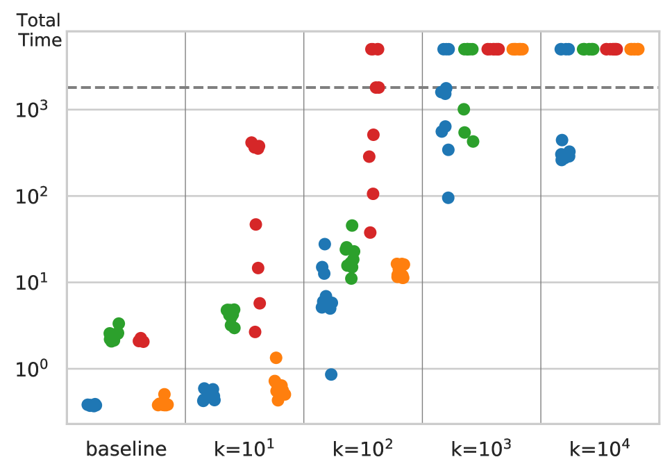
(a) $|\textsc{cfl}|=10^{1}$

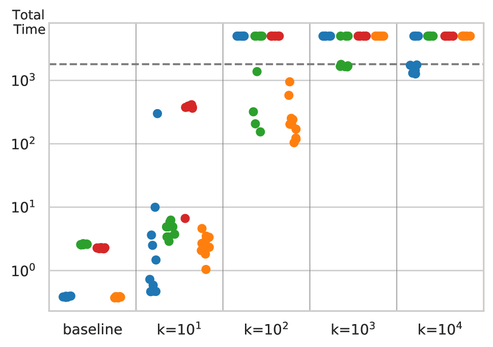
(b) $|\textsc{cfl}|=10^{2}$

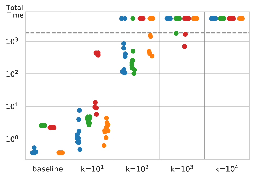
(c) $|\textsc{cfl}|=10^{3}$

Figure 2: Total execution time of the algorithms computing scf solutions for the four domains across different numbers of alternative plans $k$, with each plot corresponding to one of the CFL task sizes. Domains are represented by different colors: Grid, Barman, Openstacks, and Transport.

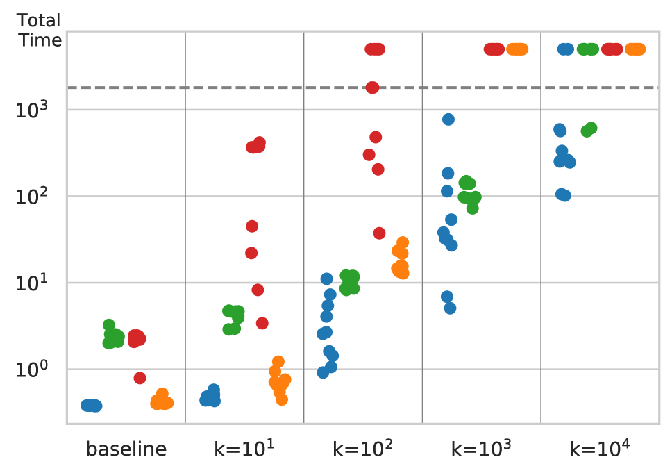
(a) $|\textsc{cfl}|=10^{1}$

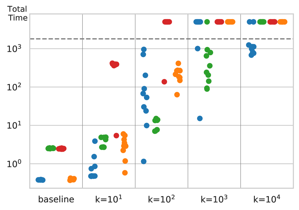
(b) $|\textsc{cfl}|=10^{2}$

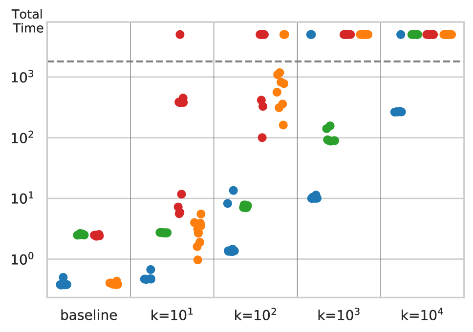
(c) $|\textsc{cfl}|=10^{3}$

Figure 3: Total execution time of the algorithms computing $\textsc{mcf}^{\bar{C}}$ solutions for the four domains across different numbers of alternative plans $k$, with each plot corresponding to one of the CFL task sizes. Domains are represented by different colors: Grid, Barman, Openstacks, and Transport.

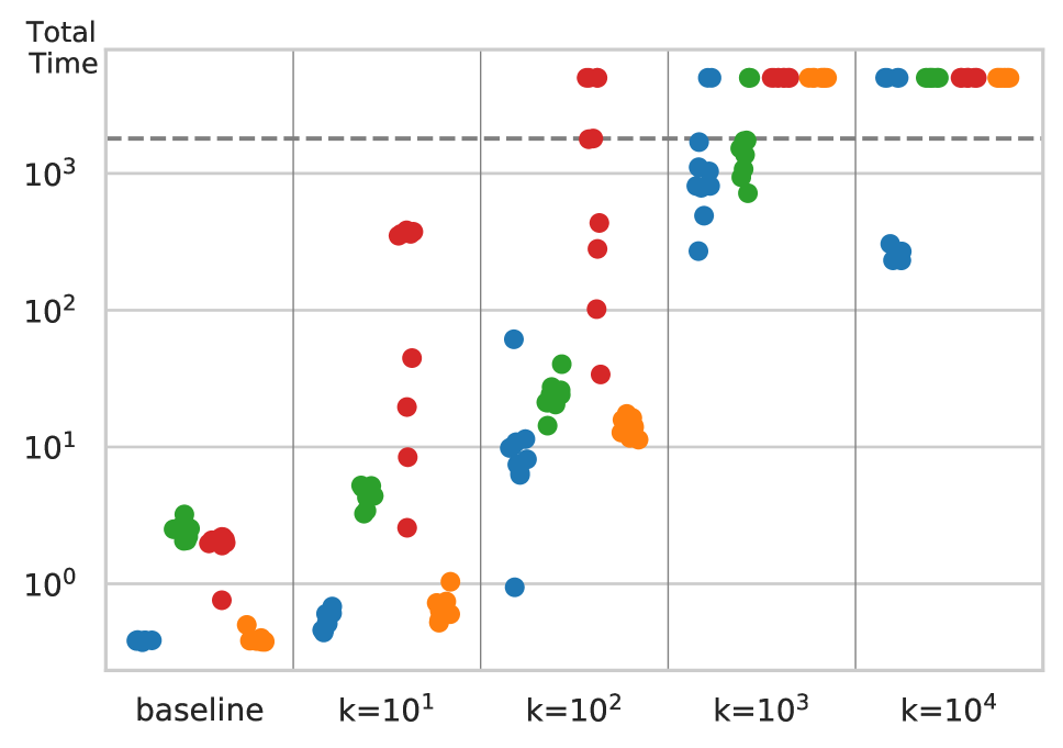
(a) $|\textsc{cfl}|=10^{1}$

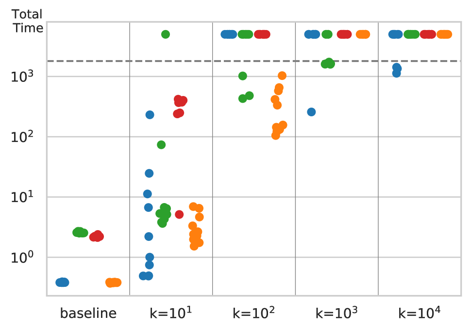
(b) $|\textsc{cfl}|=10^{2}$

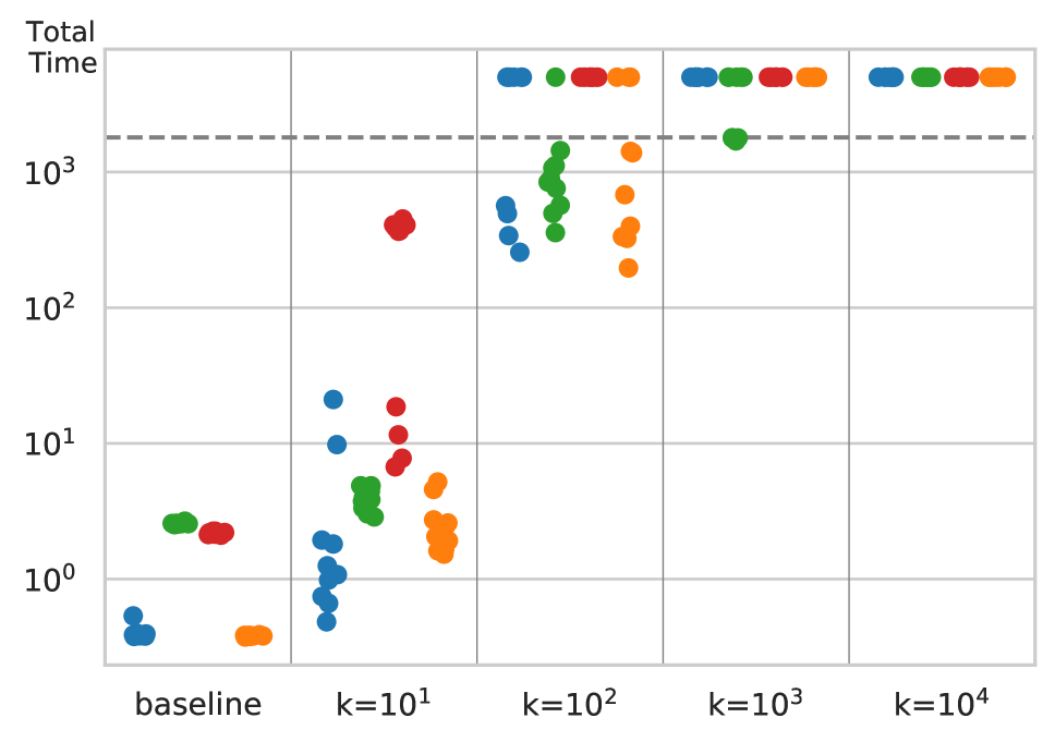
(c) $|\textsc{cfl}|=10^{3}$

Figure 4: Total execution time of the algorithms computing $\textsc{scf}^{\bar{C}}$ solutions for the four domains across different numbers of alternative plans $k$, with each plot corresponding to one of the CFL task sizes. Domains are represented by different colors: Grid, Barman, Openstacks, and Transport.

References

- Aineto, Celorrio, and Onaindia (2019) Aineto, D.; Celorrio, S. J.; and Onaindia, E. 2019. Learning action models with minimal observability. Artificial Intelligence, 275: 104–137.
- Arora et al. (2018) Arora, A.; Fiorino, H.; Pellier, D.; Métivier, M.; and Pesty, S. 2018. A review of learning planning action models. The Knowledge Engineering Review, 33: e20.
- Behnke and Bercher (2024) Behnke, G.; and Bercher, P. 2024. Envisioning a Domain Learning Track for the IPC. In ICAPS Workshop on the International Planning Competition.
- Choi and Kim (2012) Choi, J.; and Kim, K.-E. 2012. Nonparametric Bayesian inverse reinforcement learning for multiple reward functions. Advances in neural information processing systems, 25.
- Cresswell, McCluskey, and West (2013) Cresswell, S. N.; McCluskey, T. L.; and West, M. M. 2013. Acquiring planning domain models using LOCM. The Knowledge Engineering Review, 28(2): 195–213.
- Forrest and Lougee-Heimer (2005) Forrest, J.; and Lougee-Heimer, R. 2005. CBC user guide. In Emerging theory, methods, and applications, 257–277. INFORMS.
- Garrido (2023) Garrido, A. 2023. Learning cost action planning models with perfect precision via constraint propagation. Information Sciences, 628: 148–176.
- Garrido and Gragera (2024) Garrido, A.; and Gragera, A. 2024. On the difficulties for the Evaluation of Learned Planning Models. In ICAPS Workshop on Echoing Failed Efforts in Planning.
- Ghallab, Nau, and Traverso (2004) Ghallab, M.; Nau, D. S.; and Traverso, P. 2004. Automated planning - theory and practice. Elsevier. ISBN 978-1-55860-856-6.
- Gragera et al. (2023) Gragera, A.; Fuentetaja, R.; García-Olaya, Á.; and Fernández, F. 2023. A planning approach to repair domains with incomplete action effects. In Proceedings of the International Conference on Automated Planning and Scheduling, volume 33, 153–161.
- Gregory and Lindsay (2016) Gregory, P.; and Lindsay, A. 2016. Domain model acquisition in domains with action costs. In Proceedings of the International Conference on Automated Planning and Scheduling, volume 26, 149–157.
- Helmert (2006) Helmert, M. 2006. The fast downward planning system. Journal of Artificial Intelligence Research, 26(1): 191–246.
- Kambhampati (2007) Kambhampati, S. 2007. Model-lite planning for the web age masses: The challenges of planning with incomplete and evolving domain models. In Proceedings of the National Conference on Artificial Intelligence, volume 22, 1601. Menlo Park, CA; Cambridge, MA; London; AAAI Press; MIT Press; 1999.
- Lanchas et al. (2007) Lanchas, J.; Jiménez, S.; Fernández, F.; and Borrajo, D. 2007. Learning action durations from executions. In Proceedings of ICAPS Workshop on AI Planning and Learning.
- Michini and How (2012) Michini, B.; and How, J. P. 2012. Bayesian nonparametric inverse reinforcement learning. In Machine Learning and Knowledge Discovery in Databases: European Conference, ECML PKDD 2012, Bristol, UK, September 24-28, 2012. Proceedings, Part II 23, 148–163. Springer.
- Nebel, Dimopoulos, and Koehler (1997) Nebel, B.; Dimopoulos, Y.; and Koehler, J. 1997. Ignoring irrelevant facts and operators in plan generation. In European Conference on Planning, 338–350. Springer.
- Ng, Russell et al. (2000) Ng, A. Y.; Russell, S.; et al. 2000. Algorithms for inverse reinforcement learning. In Icml, volume 1, 2.
- Pozanco et al. (2023) Pozanco, A.; Papasotiriou, K.; Borrajo, D.; and Veloso, M. 2023. Combining heuristic search and linear programming to compute realistic financial plans. In Proceedings of the International Conference on Automated Planning and Scheduling, volume 33, 527–531.
- Salerno, Fuentetaja, and Seipp (2023) Salerno, M.; Fuentetaja, R.; and Seipp, J. 2023. Eliminating redundant actions from plans using classical planning. In Proceedings of the International Conference on Principles of Knowledge Representation and Reasoning, volume 19, 774–778.
- Seipp, Torralba, and Hoffmann (2022) Seipp, J.; Torralba, A.; and Hoffmann, J. 2022. PDDL Generators. In https://doi.org/10.5281/zenodo.6382174. Zenodo.
- Speck, Mattmüller, and Nebel (2020) Speck, D.; Mattmüller, R.; and Nebel, B. 2020. Symbolic top-k planning. In Proceedings of the AAAI Conference on Artificial Intelligence, volume 34, 9967–9974.
- Yang, Wu, and Jiang (2007) Yang, Q.; Wu, K.; and Jiang, Y. 2007. Learning action models from plan examples using weighted MAX-SAT. Artificial Intelligence, 171(2-3): 107–143.