Effective membership problem and systems of polynomial equations with multiple roots.

Abstract.

For a triple of convex bodies $(A,B,B)$ we solve the so called effective membership problem, i.e. for generic $f_{1},f_{2}\in\mathbb{C}^{B}$ we provide a method to compute $\mathbb{C}^{A}\cap I$, where $I=(f_{1},f_{2})$ is an ideal in the ring of Laurent polynomials. We connect this topic to the study of mixed discriminants and multiple solutions of sparse systems of equations.

1. Introduction.

1.1. Nullstellensatz and membership problem.

Classical Hilbert Nullstellensatz says that the system of polynomial equations $f_{i}=0,\ i=1,\ldots,k$ over algebraically closed field (say $\mathbb{C}$) has no solutions if and only if the ideal $(f_{1},\ldots,f_{k})$ contains unity, that is, there exists a decomposition$\colon$

(1.1) $$1=c_{1}f_{1}+\ldots+c_{k}f_{k},\ c_{i}\in\mathbb{C}[\bf{x}].$$

To find $c_{i}$ from 1.1 we would like to have some upper bound imposed on the degrees of $c_{i}$. The so called Effective Nullstellensatz is a branch of results dedicated to the problem of finding the multiples in 1.1 with the least possible degree for a given type of systems $f_{1},\ldots,f_{k}$. For example, we have the well known result [1] of W. Dale Brownawell published in 1987$\colon$

         Theorem 1.1 (W. Dale Brownawell, 1987).

Let the polynomials $P_{1},\ldots,P_{m}\in\mathbb{C}[\bf{x}]$ with $\deg P_{i}\leq D$ have no common zero in $\mathbb{C}^{n}$. Then there are polynomials $A_{1},\ldots,A_{m}\in\mathbb{C}[\bf{x}]$ with

$$\deg A_{i}\leq\mu nD^{\mu}+\mu D,$$

where $\mu=\min\{m,n\}$, such that

$$1=A_{1}P_{1}+\ldots+A_{m}P_{m}.$$

In 1988, one year later in [2] Kollar obtained a new bound for polynomials of degree at least $3$. The estimate given in the paper is sharp in the following meaning$\colon$If we have a system $f_{i}=0,\ d_{i}=\deg f_{i}\geq 3$ with no common zeroes then there exists a tuple of polynomials $c_{1},\ldots,c_{k}$ such that $1=f_{1}c_{1}+\ldots+f_{k}c_{k}$, $\deg f_{i}c_{i}\leq N(d_{1},\ldots,d_{k},k,n)$, where $N(d_{1},\ldots,d_{k},k,n)$ is a function depending only on $d_{i},k,n$. Moreover there exists a system $f^{0}_{1},\ldots,f^{0}_{k}$ with no common solutions such that there is NO set of multiples $c_{i}$ with the property $1=c_{1}f^{0}_{1}+\ldots+c_{k}f^{0}_{k}$ such that $\deg f_{i}c_{i}<N(d_{1},\ldots,d_{k},k,n)$ for at least one of $i$. Other results on the Effective Nullstellensatz were obtained in [6], [7] and [18], for example, and recently [4] which enhances theorem 1.3 below.

The estimate can be significantly improved if we consider the set of sufficiently generic systems. The first step toward this is to consider the ring of Laurent polynomials $\mathbb{C}[\bf{x},\bf{x}^{-1}]$ instead of the ordinary ring of polynomials. For example we have the following result from [3]$\colon$

         Theorem 1.2 (Canny, J., and I. Z. Emiris., 2000).

Let $A_{0},\ldots,A_{n}\subset\mathbb{Z}^{n}$ be convex polytopes. Let $A=A_{0}+\ldots+A_{n}$ be of full dimension $n$. Then there exists a Zariski open subset $U$ of the space $\mathbb{C}^{A_{0}}\oplus\ldots\oplus\mathbb{C}^{A_{n}}$ such that for any system of equations $f=(f_{0},\ldots,f_{n})\in U$ and any $g\in\mathbb{C}^{A}$ there exists a decomposition $g=c_{0}f_{0}+\ldots+c_{n}f_{n}$ with $\operatorname{supp}c_{i}\subset\sum A_{j},\ j\neq i$.

From this result we can obtaine a new version of Nullstellensatz putting $A_{i}=d_{i}E^{n}$ where $E^{n}$ is the standard n dimensional simplex and $g=1$.

In paper [8] the following was obtained$\colon$

         Theorem 1.3 (J. Tuitman, 2011).

Let $A_{0},\ldots,A_{n}\subset\mathbb{Z}^{n}$ be convex polytopes and $f=(f_{1},\ldots,f_{k})\in\mathbb{C}^{A_{0}}\oplus\ldots\oplus\mathbb{C}^{A_{n}}$. Let $A=A_{0}+\ldots+A_{n}$ be of full dimension $n$. Then $f$ is non-degenerate if and only if for any $g\in\mathbb{C}^{A}$ there exists a decomposition $g=c_{0}f_{0}+\ldots+c_{k}f_{k}$ with $\operatorname{supp}c_{i}\subset\sum A_{j},\ j\neq i$.

In this theorem and in the classical paper [9] the same definition of non-degeneracy is used. We will remind it now. For a given polytope $A\subset\mathbb{R}^{n}$ and $v\in\mathbb{R}^{n}$ we denote $A(v)$ to be the subset $\{a|v.a=\min_{x\in A}{v.x}\}$ of $A$. For a given polynomial $f=\sum f_{p}\bf{x}^{p}$ and a subset $A\subset\mathbb{Z}^{n}$ we denote by $f|_{A}$ the new polynomial $\sum f_{p}\bf{x}^{p}$, where the sum is only taken for $p\in A\cap\operatorname{supp}f$. We call the tuple of equations $f_{i}=0$ non-degenerate with respect to the set of polytopes $A_{i}$ if the corresponding system $f_{i}|_{A_{i}(v)}=0$ has no solutions for any direction $v\neq 0$.

We see that all results formulated above allow us to reduce the problem of finding the multiples in the decomposition 1.1 to the problem of solving a system of linear equations.

Let us introduce another problem closely related to the topic. Let $A,B_{1},\ldots,B_{k}$ be subsets of $\mathbb{Z}^{n}$. For a tuple of polynomials $f=(f_{1},\ldots,f_{k})\in\mathbb{C}^{B_{1}}\oplus\ldots\oplus\mathbb{C}^{B_{k}}$, we have the ideal $I_{f}$ generated by $f$ in the ring of polynomials. The question is what we can say about the set of polynomials that are members of $I_{f}$ and have support in $A$. We denote$\colon$

$$\mathcal{V}_{A}^{f}=I_{f}\cap\mathbb{C}^{A}.$$

and

$$\mathcal{V}_{A}^{I}=I\cap\mathbb{C}^{A},\text{for an ideal}\ I.$$

         Example 1.4.

Take $f=1+x\in\mathbb{C}[x]$ and $A=\{0,2\}$. We can easily compute that $\mathcal{V}_{A}^{f}=\{c(1-x^{2}),\ c\in\mathbb{C}\}$.

In general $\mathcal{V}_{A}^{f}$ is always a finite dimensional vector space. We arrive at the problem how to compute $\dim\mathcal{V}_{A}^{f}$ in terms of $A,B$ for generic $f\in\mathbb{C}^{B}$. For example we have the following simple fact$\colon$

         Proposition.

If $A$ is a convex polytope in $\mathbb{Z}^{n}$ then $\dim\mathcal{V}_{A}^{f}=|A\ominus B|$ for generic $f\in\mathbb{C}^{B}$. Here $A\ominus B=\{b\in\mathbb{Z}^{n}|b+B\subset A\}$.

If $A$ has some holes (see example 1.4) then of course $\mathcal{V}_{A}^{f}\neq\mathbb{C}^{A\ominus B}$. But it is still true that $\mathcal{V}_{A}^{f}$ is a subspace of $\mathbb{C}^{\operatorname{conv}(A)\ominus B}$. For several $B$ the situation is getting more interesting.

         Example 1.5.

Consider the tuple $(A,A\cup\{q\},A\cup\{q\})$. Then a pair of polynomials supported at $A\cup\{q\}$ can be written in the form $f_{1}=f^{0}_{1}+\alpha_{1}{\bf{x}}^{q},\ f_{2}=f^{0}_{2}+\alpha_{2}{\bf{x}}^{q}$, where $f^{0}_{1}$ and $f^{0}_{2}$ are supported at $A$. We can see that $f_{1}\alpha_{2}-f_{2}\alpha_{1}\in\mathbb{C}^{A}$ so $\mathcal{V}^{f}_{A}$ is not empty, but $A\ominus(A\cup\{q\}))=A\ominus(A\cup\{q\}))=\varnothing$.

We give two strongly related definitions, first of which we have already seen. Let as before $I$ be an ideal generated by the tuple of functions $f=(f_{1},\ldots,f_{n-1})$. For $X\subset\mathbb{R}^{n}$ we denote $X\cap\mathbb{Z}^{n}$ by $\mathbb{Z}(X)$.

         Definition 1.6.

Let $C=(C_{1},\ldots,C_{n-1})$, $C_{i}\subset\mathbb{Z}^{n}$. We denote by $\mathcal{V}^{C,I}_{A}$ the following space$\colon$

$$\mathcal{V}^{C,\ I}_{A}=\{g\in I|\ \exists(c_{1},\ldots,c_{n-1})\ \text{s.t.}\ g=c_{1}f_{1}+\ldots+c_{n-1}f_{n-1}\ \text{and}\ c_{i}\in\mathbb{C}^{C_{i}}\}\cap\mathbb{C}^{A}$$

It’s easy to see that $\mathcal{V}^{I}_{A}=\mathcal{V}^{\mathbb{Z}^{n},\ I}_{A}$

The difference between these two is that $\mathcal{V}_{A}^{I}$ is a space of all members of $I$ with given support $A$ and $\mathcal{V}^{C,I}_{A}$ is a space of all members who can be expressed in the form $c_{1}f_{1}+\ldots+c_{n-1}f_{n-1}$ and all the supports of $c_{i}$ are also restricted by a given subset.

The dimension of $\mathcal{V}^{(f_{1},...,f_{n-1})}_{A}$ does not depend on the choice of a generic system based on $B$ so we will write $\dim\mathcal{V}^{B}_{A}$ instead of $\dim\mathcal{V}^{(f_{1},...,f_{n-1})}_{A}$ for generic $(f_{1},...,f_{n-1})\in\mathbb{C}^{B}$.

Since $\dim\mathcal{V}_{A}^{B}$ is finite, it is easy to see that there exists $C^{0}=(C^{0}_{1},\ldots,C^{0}_{n-1})$, $C_{i}\subset\mathbb{R}^{n}$ s.t. $\mathcal{V}^{\mathbb{Z}(C),I}_{A}=\mathcal{V}^{I}_{A}$. We will also use that obviously $\dim\mathcal{V}_{A}^{B}=\dim\mathcal{V}_{A+u}^{B+v}$ for any $u,\ v\in\mathbb{Z}^{n}$. The aim of effective membership problem is to find such $C^{0}$ for prescribed set of functions generating $I$. If $C^{0}$ satisfies this property we will call it foundation.

Let us formulate in details the main result proven in the section 7$\colon$

         Theorem 1.7.

Let $(A,B,B)$ be a triple of polytopes in $\mathbb{Z}^{n}$. Let $t\in\mathbb{R},\ t>1$ and $v\in\mathbb{Z}^{n}$ s.t. $A+v\subset\mathbb{Z}((t+1)B)$. Then $(tB,tB)$ is a foundation for $(A,B,B)$.

We will also prove the refinement of theorem 1.7 for small $A$.

         Theorem 1.8.

Let $(A,B,B)$ be a triple of polytopes in $\mathbb{Z}^{n}$ such that $B$ is not a segment. And there exists $v\in\mathbb{Z}^{n}$ and $t\in\mathbb{R},\ t\in(0,1]$ such that $v+A\subset tB$. Then $(\{0\},\{0\})$ is a foundation for $(A,B,B)$.

Summarising theorems 1.7 and 1.8 we obtain the main result of the paper

         Theorem 1.9.

Let $(A,B,B)$ be a triple of convex bodies in $\mathbb{Z}$. Let $A$ be arbitrary and $B$ be not a segment. Let $t\in\mathbb{R},\ t\geq 0$ be such that $A\subset\mathbb{Z}((t+1))B)$. Then $(tB,tB)$ is a foundation for $(A,B,B)$.

In particular, from the final theorem it follows that $\dim\mathcal{V}_{A}^{A}=2$.

Results similar to 1.9 were obtained in [22], [23] (Theorem 3) in somewhat different settings. We generalise Theorem 1.2. from [22] in the case $m=2$.

         Theorem 1.10.

[E. Wulcan, 2011] Let $F_{1},\ldots,F_{m}$, and $\Phi$ be polynomials in $\mathbb{C}[z_{1},\ldots,z_{n}]$ and let $P$ be a smooth and “large” polytope that contains the origin and the support of $\Phi$ and the coordinate functions $z_{1},\ldots,z_{n}$. Assume that $\Phi\in(F_{1},\ldots,F_{m})$ and moreover that the codimension of the zero set of the $F_{j}$ is $m$ and that it has no component contained in the variety at infinity. Then there are polynomials $G_{j}$ such that

$$\sum F_{i}G_{i}=\Phi$$

and

$$\operatorname{supp}(F_{j}G_{j})\subset P.$$

Descriptions of ‘large’ and ‘has no components at infinity’ are given in the original paper. The main difference between 1.10 and 1.9 is that we do not assume smoothness of the polytope. A polytope of any dimension $n$ is called smooth if each vertex is contained in precisely $n$ edges and the set of corresponding $n$ primitive vectors forms a lattice basis.

To demonstrate the main idea of the proof of theorem 1.7, in section 4 we will consider the simplified construction similar to what we are going to do later, in section 7, in more general settings.

1.2. Study of discriminants.

The space $\mathcal{V}^{f}_{A}$ defined above plays an important role in the study of discriminant. For the convenience of the reader let us give some basic explanations. The discriminant of a polynomial with the support $A$ is the closure of the set $\triangle_{A}=\{f\in\mathbb{C}^{A}|\ df=f=0\ \text{has a solution}\}$. The discriminant variety $\triangle_{A}=0$ is projectively dual to the toric variety $X_{A}$ [10] (p.3), that in particular can be defined as follows$\colon X_{A}$ is the closure of the image of $(\mathbb{C}^{*})^{n}$ by the so-called monomial map $m_{A}$

$$m_{A}\colon(\mathbb{C}^{*})^{n}\rightarrow\mathbb{CP}^{A}$$

$$x\mapsto[\ldots\colon x^{a_{i}}\colon\ldots].$$

The notion of the discriminant can also be applied to systems of several polynomial equations. For $k=n$ i.e. the case when the number of equations and variables are equal to each other, we have the following classical result$\colon$

         Theorem 1.11.

Bernstein–Kushnirenko formula

For a generic system of polynomial equations $f_{1}=\ldots=f_{n}$ in $n$ complex variable the number of its solutions on the complex torus $(\mathbb{C}^{*})^{n}$ is equal to $n!\operatorname{MV}(A_{1},\ldots,A_{n})$ where $A_{i}$ is the Newton polytope of the corresponding equation and $\operatorname{MV}$ is the mixed volume.

A system has a singular solution if at some point $p$ we have $f(p)=0$ and $df_{1}(p),\ldots,df_{n}(p)$ are linearly dependent. A system $f=0,f\in\mathbb{C}^{A}$ will be called degenerate if it has a singular root itself or $f_{i}|_{A_{i}(v)}=0$ has it for some direction $v\in\mathbb{R}^{n}$. The set of all such systems lies in an algebraic subset of the space of parameters $\mathbb{C}^{A}=\mathbb{C}^{A_{1}}\oplus\ldots\oplus\mathbb{C}^{A_{n}}$.

We define the mixed discriminant of a tuple $A=(A_{1},\ldots,A_{k})$ as the closure in $\mathbb{C}^{A}$ of the set of all degenerate systems.

Discriminants of one general polynomial of several variables with a prescribed Newton polytope were first systematically studied in [10]. The generalization to two or more general polynomial equations is studied starting from [12] and [13].

In the work [11] it was shown that for sufficiently good $A$ a generic point on the discriminant corresponds to the system with the unique degenerate root which has multiplicity 2. By sufficiently good we mean the following characterisations$\colon$

         Definition 1.12.

A tuple of finite sets $X_{1},\ldots,X_{k}$ in $Z^{n}$ is said to be reduced, if they cannot be shifted to the same proper sublattice of $Z^{n}$.

For most of $A$ there are systems that have a root of higher multiplicity. Let us denote by $C_{k}$ the set of all systems that have a root of multiplicity $k$. We expect that $C_{k+1}$ has codimension 1 in the previous one. Natural problems that arise here are$\colon$

1. Classify all $A$ for which $C_{k}$ is empty for some low $k$.

2. What properties should $A$ satisfy to make $C_{k}$ of expected codimension?

3. Estimate the length of maximal possible chain of non empty consecutive strata.

$$C_{k},C_{k-1},\ldots,C_{0}.$$

For example, if $\operatorname{MV}(A)=2$ the strata $C_{k}$ will be empty for $k\geq 3$. The third question is not trivial since there exist tuples with a system who has root of multiplicity $l$ and with a system who has root of multiplicity $l+2$ but for this tuple there is no system with multiplicity $l+1$. For example take bodies depicted below on fig.1. A system supported on the following pair of bodies have no root of multiplicity $5$, though it can have a root of multiplicity $4$ and $6$.

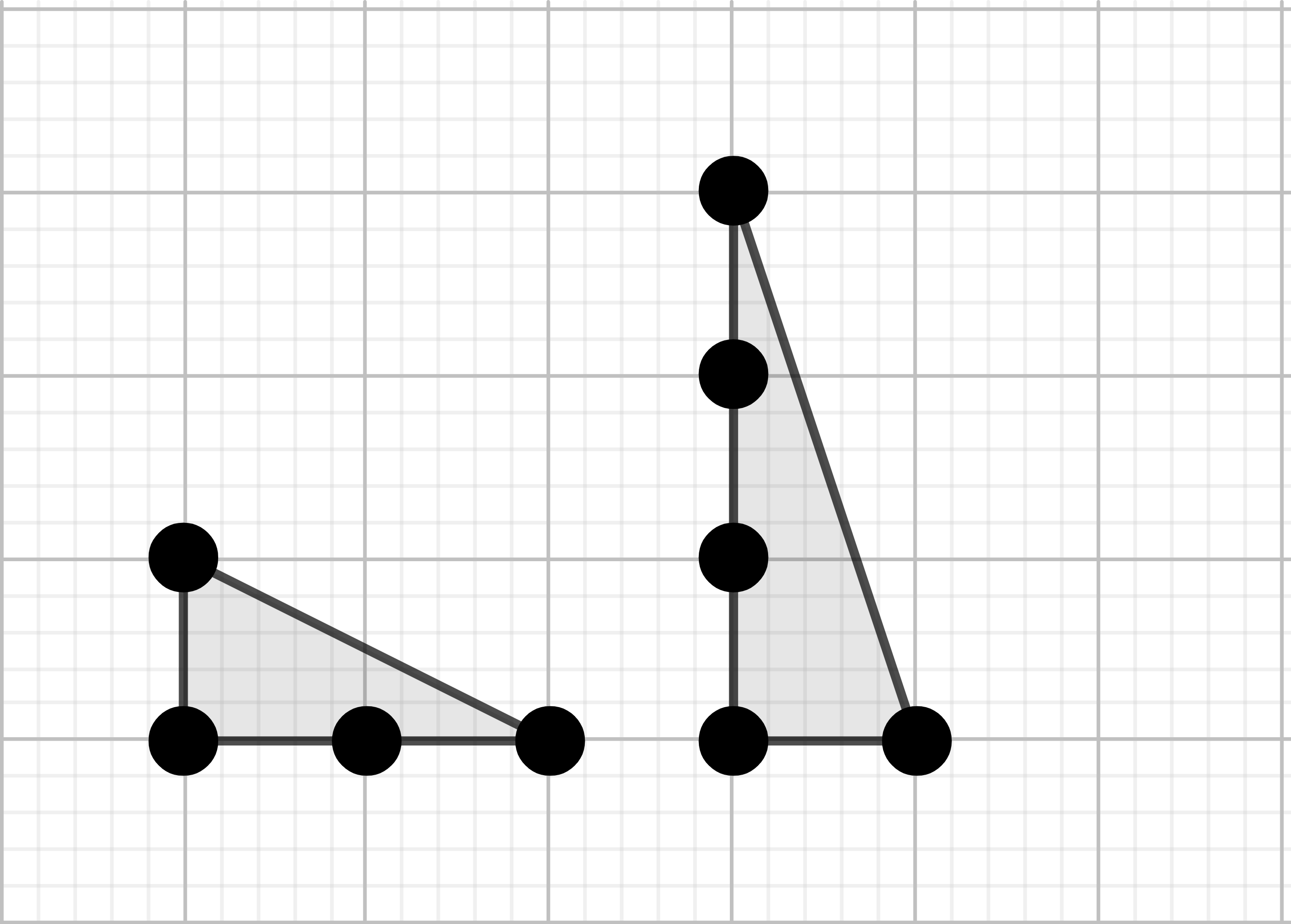
Figure 1. tuple with discontinues chain of strata

For $k=2,n=d$ these problems were solved in [14] and [11], which lead to new results on the Galois groups of general systems of polynomial equations. From the results of the work [15] it follows that the maximal possible $k$ such that $C_{k}$ is non empty can be bounded from above by a function depending on the total number of monomials in $A$ but not on their degrees. In this direction some new interesting results were obtained in [5]. Namely, for a system in $n$ variables of $n$ equations with the same support set $A$, the highest possible multiplicity of an isolated root was estimated in terms of the decomposition $|A|=n+m+1$. Also, in the recent work [17] it was shown that the only smooth polygons $A$ such that curves $\{f=0\},\,f\in\mathbb{C}^{A}$, may have at most $A_{1}$-singularities, are equivalent to the 2–simplex or a unit square.

The aim of this paper is to bring together two topics described above. We are ready to show the meaning of $\mathcal{V}_{A}^{f}$ to the studying of discriminants. We begin with a well known result from the differential geometry of curves$\colon$

         Theorem 1.13.

Let $\gamma$ be a projective curve that is given locally (in some neighbourhood $U$ of a generic point $p\in\gamma$) by a family of holomorphic functions$\colon$

$$\phi\colon U\rightarrow\mathbb{P}^{n}$$

$$z\mapsto[\ldots\colon\phi_{i}(z)\colon\ldots].$$

If the dimension of the projective hull of $F$ equals $k$, then there exists a descending chain of pencils of osculating hyperplanes

$$V^{0}\supset V^{1}\supset V^{2}\supset\ldots\supset V^{k},$$

such that hyperplanes lying in $V^{i}$ intersect $F$ at p with multiplicity at least $i$, and $\dim V^{i}-\dim V^{i-1}=1$. In fact, $V^{i}$ contains a dense subset of hyperplanes that intersect $\gamma$ with multiplicity exactly $i$ and a proper subspace of hyperplanes that intersect $\gamma$ with multiplicity at least $i+1$ for $i<k$, and $V^{k}$ contains a unique hyperplane that intersects $\gamma$ with multiplicity $k$.

For the sake of readability, we will prove it in the next section, as a proposition. Now, we apply it to the system of $n$ polynomial equations with $n$ variables. Again, let us consider the monomial map$\colon$

$$m_{A}\colon(\mathbb{C}^{*})^{n}\rightarrow\mathbb{CP}^{A}$$

$$x\mapsto[\ldots\colon x^{a_{i}}\colon\ldots].$$

Consider a system $f=\{f_{1}=\ldots=f_{n-1}=0\}$ such that all polynomials are generic. Assume that $f_{i}\in\mathbb{C}^{B_{i}}$. This system defines a smooth curve $F$ on the complex torus $(\mathbb{C}^{*})^{n}$.

The map $m_{A}$ is well defined on $(\mathbb{C}^{*})^{n}$. We denote $m_{A}((\mathbb{C}^{*})^{n})$ by $\mathbb{T}$. Let $g=\sum_{a\in A}c_{a}x^{a}$ be a polynomial supported at $A$. By $\pi_{g}$ we denote the hyperplane in $\mathbb{CP}^{A}$ given by the linear form $\sum_{a\in A}c_{a}z_{a}$, i.e. $\pi_{g}$ has the same coefficients as $g$ has. Assume that the projective hull of $m_{A}(F)$ has dimension $k$. Then, according to the theorem 1.13 at the generic point $p$ of $m_{A}(F)$ we have a set of hyperplanes $H_{i}$, $i=0,\ldots,k$ in $\mathbb{CP}^{A}$ such that $\pi_{i}$ intersects $m_{A}(F)$ at $p$ with multiplicity $i$.

In the next section we will prove that $k=|A|-\dim\mathcal{V}_{A}^{f}-1$ and it does not actually depend on the choice of a generic curve $F$ supported at $B$. Moreover the intersection multiplicity of $\pi_{i}$ and $m_{A}(F)$ at $p$ is equal to the intersection multiplicity of $F$ and the hypersurface $f_{n}^{i}$ which corresponds to the hyperplane $\{\pi_{i}=0\}$.

One of the main results given in this paper is$\colon$

         Theorem 1.14.

Let $A,B_{1},\ldots,B_{n-1}\subset\mathbb{Z}^{n}$ be a tuple of polytopes such that $\operatorname{MV}(A,B_{1},\ldots,B_{n-1})>0$. Then for almost all points $p$ on a generic curve $\gamma=\{f=0\}$ supported at $B$, there exists a set of osculating curves $g_{i}$ supported at $A$, such that $g_{i}$ intersects $\gamma$ at $p$ with multiplicity $i$ for any $i\leq|A|-\dim\mathcal{V}_{A}^{f}-1$, i.e. the multiplicity of the root $p$ of the system $f=g_{i}=0$ is $i$.

In fact we can derive from here that the mixed discriminant of the tuple $(A,B)$ admits a chain of consecutive non empty strata of expected dimension. This stratification depends on the order of the support sets so in fact we have several good stratifications. We will do it in section 3.

In sections 5 and 6 we are working on the technical tools designed to justify the major steps of the proof of Theorem 1.9. In section 7 we prove it and develop the theory of computing $\mathcal{V}_{A}^{f}$ in dimension 3 for arbitrary $A$ in a particular case $B_{1}=B_{2}$. In the end, in additional section we proof the inequality $|A+B|+|A\ominus B|\geq 2|A|$ in dimension 2 for any convex $A,B\subset\mathbb{Z}^{2}$.

2. Proof of 1.14.

In this section we prove theorem 1.14 and 1.13. Let us introduce some notation. Recall that for each $a=(a_{1},\ldots,a_{n})\in\mathbb{Z}^{n}$ we use the expression $z^{a}$ to denote the monomial $z_{1}^{a_{1}}\ldots z_{n}^{a_{n}}$, where $z_{i}\in\mathbb{C}^{*}$ and for each $A\subset\mathbb{Z}^{n}$ we denote by $\mathbb{C}^{A}$ the space of Laurent polynomials $\sum_{a\in A}c_{a}z^{a}$ supported at $A$. For any polynomial $f$ the convex hull of its support is called the Newton polytope of $f$. For a tuple of subsets $S=(A_{1},\ldots,A_{k})\subset\mathbb{Z}^{n}$, we have $\mathbb{C}^{S}=\mathbb{C}^{A_{1}}\oplus\ldots\oplus\mathbb{C}^{A_{k}}$. We identify each $f=(f_{1},\ldots,f_{k})\in\mathbb{C}^{S}$ with the corresponding system of polynomial equations $f_{1}=\ldots=f_{k}=0$. For any two subsets $A,B$ of $\mathbb{Z}^{n}$ their Minkowski sum $A+B$ is defined as follows$\colon A+B=\{a+b|a\in A,b\in B\}\subset\mathbb{Z}^{n}$. We say that a finite subset $A\subset\mathbb{Z}^{n}$ is convex if it can be represented in the form $A=\mathbb{Z}^{n}\cap\bar{A}$, for some convex $\bar{A}\subset\mathbb{R}^{n}$.

As it was promised, we give here a proof of 1.13

Proof.

Let the dimension of the projective hull of $\gamma$ be equal to $k$. Without loss of generality we may assume that $\gamma$ lies in the projective space of dimension $k$ and is not contained in any hyperplane. The latter implies that coordinate functions $\phi_{i}(z)$ are linearly independent. It is well known that any set of analytic functions is linearly independent if and only if the Wronskian of this set is not identically 0. Recall that the Wronskian can be computed by the following formula

$$\det\begin{bmatrix}\phi_{0}&\phi_{1}&\phi_{2}&\dots&\phi_{k}\\ \phi_{0}^{(1)}&\phi_{1}^{(1)}&\phi_{2}^{(1)}&\dots&\phi_{k}^{(1)}\\ {5}\\ \phi_{0}^{(k)}&\phi_{1}^{(k)}&\phi_{2}^{(k)}&\dots&\phi_{k}^{(k)}\end{bmatrix}.$$

If at some point of the curve the Wronskian vanishes, we will say that this point is Weierstrass, it can be shown that the property of being Weierstrass is invariant with respect to the choice of holomorphic parametrization. Now let us provide a relation between that property and the statement of the Lemma. Expand each $f_{i}$ as a Laurent power series at $p$ and substitute them into the expression $H(x_{0},\ldots,x_{k})=c_{0}x_{0}+c_{1}x_{1}+\ldots+c_{n}x_{n}$. Regrouping the terms by their exponents $z^{i}$ we obtain$\colon$

$$H(\phi_{0}(z),\ldots,\phi_{k}(z))=z^{0}(c_{0}\phi_{0}(0)+\ldots+c_{k}\phi_{k}(0))/0!+$$

$$z^{1}(c_{0}\phi_{0}^{(1)}(0)+\ldots+c_{k}\phi_{k}^{(1)}(0))/1!+\ldots$$

$$z^{j}(c_{0}\phi_{0}^{(j)}(0)+\ldots+c_{k}\phi_{k}^{(j)}(0))/j!+\ldots$$

$$z^{k}(c_{0}\phi_{0}^{(k)}(0)+\ldots+c_{k}\phi_{k}^{(k)}(0))/k!.$$

The curve $\gamma$ and the hyperplane $\{H=0\}$ intersect with multiplicity $i$ at $p$ if and only if
$\bar{H}(z)=H(\phi_{0}(z),\ldots,\phi_{k}(z))=cz^{i}+h.o.t.,c\neq 0$. We list the first $k+1$ coefficients of the expansion $\bar{H}(z)$ in the following matrix$\colon$

$$A=\begin{bmatrix}\phi_{0}(0)&\phi_{1}(0)&\phi_{2}(0)&\dots&\phi_{k}(0)\\ \phi_{0}^{(1)}(0)&\phi_{1}^{(1)}(0)&\phi_{2}^{(1)}(0)&\dots&\phi_{k}^{(1)}(0)\\ {5}\\ \phi_{0}^{(k)}(0)&\phi_{1}^{(k)}(0)&\phi_{2}^{(k)}(0)&\dots&\phi_{k}^{(k)}(0)\end{bmatrix}.$$

As we can see, the matrix $A$ is indeed the Wronskian of the system of functions $\{\phi_{i}\}$ at zero. Since $\gamma$ does not lie in any hyperplane, the Wronskian matrix is not identically zero. Switching from $p$ to another point $q\in U$ if necessary, we conclude that $A$ has maximal rank. To finish the proof, we choose $V^{i}$ to be the set of hyperplanes corresponding to solutions of the first $i$ rows of $A$. ∎

By $\mathbb{CP}^{A}$ we denote the projective space whose homogeneous coordinates are enumerated by $A$. We denote the zero set of an ideal or a set of polynomials by $\mathcal{Z}(\ldots)$. We say that a curve $F$ is supported at $B=(B_{1},\ldots,B_{n-1})\subset\mathbb{Z}^{n}$ if there exists $f\in\mathbb{C}^{B}$ such that $F=\mathcal{Z}(f)$. The number of points in the set $A$ is denoted by $|A|$. The mixed volume of convex polytopes $A,B_{1},\ldots,B_{n-1}$ is denoted by $\operatorname{MV}(A,B_{1},\ldots,B_{n-1})$.

The monomial map is denoted by $m_{A}$ just like in the previous section. Let $g=\sum_{a\in A}c_{a}x^{a}$ be a polynomial supported at $A$. By $\pi_{g}$ we denote the hyperplane in $\mathbb{CP}^{A}$ given by the linear form $\sum_{a\in A}c_{a}z_{a}$, i.e. $\pi_{g}$ has the same coefficients as $g$ has. The next lemma explains the correspondence between hyperplanes in $\mathbb{CP}^{A}$ containing $m_{A}(F)$ and hypersurfaces in $(\mathbb{C}^{*})^{n}$ which contain $F$.

         Lemma 2.1.

Let $A,B_{1},\ldots,B_{n-1}$ be a tuple of subsets in $\mathbb{Z}^{n}$. Then there exists a dense subset $X\subset\mathbb{C}^{B}$ such that for any $f\in X$ and for any $g\in\mathbb{C}^{A}$ the following conditions are equivalent$\colon$

1. $m_{A}(\mathcal{Z}(f))$ is contained in $\pi_{g}$;

2. $g\in I_{f}$.

Proof.

($\Rightarrow$)Let $f\in\mathbb{C}^{B}$. From [16] (Theorem 1) it follows that for almost all tuples of coefficients of the system $f=0$, the scheme $\mathbb{C}[x]/(I_{f})$ is smooth. By definition, it means that for any point $q\in\mathcal{Z}(f)$, the corresponding local ring $(\mathbb{C}[x]/(I_{f}))_{q}$ is regular and thus by Auslander–Buchsbaum theorem it is a unique factorisation domain, in particular it is reduced and so is $\mathbb{C}[x]/(I_{f})$. We denote the set of all such $f$ by $X$. Choose arbitrary $x\in\mathcal{Z}(f)$ and denote $m_{A}(x)$ by $p$. Since $p\in\pi_{g}$ we have $\sum c_{a}x^{a}=0$ therefore $x\in\mathcal{Z}(g)$ and $\mathcal{Z}(f)\subset\mathcal{Z}(g)\Rightarrow$ by Hilbert nullstellensatz for Laurent polynomials $g^{r}\in I_{f}$ for some natural $r$. Since $I_{f}$ is radical, $r$ can be chosen to be 1. ($\Leftarrow$)For the other implication, let $g=c_{1}f_{1}+\ldots+c_{n-1}f_{n-1}$, then the vanishing set of $f$ vanishes $g$ as well hence $\mathcal{Z}(f)\subset\mathcal{Z}(g)$. Therefore $m_{A}(\mathcal{Z}(f))\subset\pi_{g}$ . ∎

From lemma 2.1 it immediately follows that $|A|-\mathcal{V}_{A}^{B}-1$ is equal to the dimension of the projective hull of $m_{A}(\mathcal{Z}(f))$ for generic $f$ supported at $B$. Now, we will prove theorem 1.14

Proof.

Let $F=\mathcal{Z}(f)$ be a smooth curve supported at $B$. Since $\operatorname{MV}(A,B_{1},\ldots,B_{n-1})$ is the number of isolated roots of a generic system supported at $(A,B)$ we can see that the number of intersections of $m_{A}(F)$ and a generic hyperplane in $\mathbb{P}^{A}$ is positive and hence $m_{A}|_{F}$ is not degenerate and $\overline{m_{A}(F)}$ is an algebraic curve. Consider a generic point $p$ of $m_{A}(F)$ (generic here means non-Weierstrass point and not the image of a branch point). Let the dimension of the projective hull of $m_{A}(F)$ be $k$. Since $p$ is non-Weierstrass then by Theorem 1.13, there exists a tuple of osculating hyperplanes $\{H_{i}\}_{i=0}^{k}$ such that $H_{i}$ intersects $m_{A}(F)$ at $m_{A}(p)$ with multiplicity $i$. We denote the coefficients of these hyperplanes by $H_{a}^{i}$. Since $F$ is a smooth curve and $p$ is not the image of a branch point of $m_{A}|_{F}$, we can choose a holomorphic parametrization in some neighbourhood of $p\colon z_{i}=z_{i}(t)$. For each $i\in\{0,\ldots,k\}$ define $g_{i}=\sum_{a}H_{a}^{i}z^{a}\in\mathbb{C}^{A}$, $G_{i}=\mathcal{Z}(g_{i})$. Substitute $z_{i}(t)$ into the equation of $g$, and write the Laurent series for $g$

$$g=g_{m}t^{m}+h.o.t.$$

where $m$ is the intersection multiplicity of $F$ and $G_{i}$ at $p$. Let $L$ be a linear form not vanishing at $m_{A}(p)$. Then $\sum_{a}H_{a}^{i}z_{a}/L$ is a meromorphic function that has the same order at $m_{A}(p)$ as $g$ has at $p$. Indeed, substituting $z_{i}(t)$ into the function $\sum_{a}H_{a}^{i}z_{a}/L$ we will obtain $(g_{m}t^{m}+h.o.t.)/(c_{0}+c_{1}t^{l}+h.o.t.),c_{0},c_{1}\neq 0,l>0$. Thus we have the Laurent expansion of the following form

$$(g_{m}t^{m}+h.o.t.)/(c_{0}+c_{1}t^{l}+h.o.t.)=c^{-1}_{0}(g_{n}t^{n}+h.o.t.)(1-c_{1}c^{-1}_{0}t^{l}+h.o.t.)=c^{-1}_{0}g_{m}t^{m}+h.o.t.$$

Therefore, the intersection multiplicities of $F$ and $G_{i}$ at $p$ and $m_{A}(F)$ and $H^{i}$ at $m_{A}(p)$ are both equal to $i$ as desired. ∎

3. Strata of the dual variety of a projective curve.

In this section we describe the structure of the incidence space of curves and osculating hyper-surfaces with given support, that was introduced in the previous sections. We show that the natural stratification of this space corresponds to the stratification of the discriminant variety in one of its irreducible components. Let $\Gamma$ be a projective curve that is given locally (in some neighbourhood $U$ of a generic point $p\in\Gamma$) by a family of analytic functions$\colon$

$$\phi\colon U\rightarrow\mathbb{P}^{n}$$

$$z\mapsto[\ldots\colon\phi_{i}(z)\colon\ldots].$$

Let the dimension of the projective span of $\Gamma$ equal $k$. It is well known that any set of analytic functions is linearly independent if and only if the Wronskian of this set is not identically 0. Recall that the Wronskian can be computed by the following formula

$$\det\begin{bmatrix}\phi_{0}&\phi_{1}&\phi_{2}&\dots&\phi_{k}\\ \phi_{0}^{(1)}&\phi_{1}^{(1)}&\phi_{2}^{(1)}&\dots&\phi_{k}^{(1)}\\ {5}\\ \phi_{0}^{(k)}&\phi_{1}^{(k)}&\phi_{2}^{(k)}&\dots&\phi_{k}^{(k)}\end{bmatrix}.$$

With the Wronskian matrix, it can be easily shown that the coefficients of the osculating hyperplanes of tangency $i=0,\ldots,k$ depends holomorphicaly on $z$ in some neighbourhood of $p$, e.g. [21]. If $p=p(\omega),\omega\in U$ is a point on the curve viewed as a holomorphic function of one complex variable and $\phi$ is some fixed embedding we denote by $W_{\phi}(\omega)$ the determinant of the Wronskii matrix as a function of $\omega$. We would like to apply all this Machinery to the curve supported at $B$ embedded into projective space via $m_{A}$.

Let $I=(f_{1},\ldots,f_{n-1})\subset\mathbb{C}[\ldots,z^{\pm}_{i},\ldots],f_{i}\in\mathbb{C}^{B_{i}}$ be an ideal generated by polynomials supported at $B$ and $g$ be a polynomial supported at $A$. Assume that $g\in I$. We know that for a given $f$ the set of all such $g$ is a finite-dimensional vector space over $\mathbb{C}$. We denote this vector space by $\mathcal{V}_{A}^{I}$ according to the agreement established in the introductory section. For generic $f$, $\dim\mathcal{V}^{I}_{A}$ does not depend on the choice of $I$. So, we ignore $I$ in the expression $\mathcal{V}^{I}_{A}$ and use $\mathcal{V}^{B}_{A}$ instead. Let $\Gamma=\overline{m_{A}(\mathcal{Z}(f))}$.

There exists an algebraic subset $\triangle_{B}\subset\mathbb{C}^{B}$ such that for any curve $\{f=0\}$ in the complement of $\triangle_{B}$ we have $\dim\mathcal{V}_{A}^{I_{f}}=\dim\mathcal{V}_{A}^{B}$.

Let $p\in\Gamma$. We will call $p$ flag generic if it is smooth and non-Weierstrass. Consider the incidence sets

$$\Sigma=\{(p,f,g)|\ m_{A}(p)\in\Gamma\ \text{is flag generic},\ f\notin\triangle_{B},\ T_{p}(\Gamma)\subset\mathcal{Z}(H_{g})\}\subset(\mathbb{C}^{*})^{n}\times\mathbb{C}^{B}\times\mathbb{C}^{A}$$

$$\Sigma_{0}=\{(p,f)|\ m_{A}(p)\in\Gamma\ \text{is flag generic},\ f\notin\triangle_{B}\}\subset(\mathbb{C}^{*})^{n}\times\mathbb{C}^{B}$$

We have natural projections

by definition $\forall f\in\mathbb{C}^{B}\setminus\triangle_{B}$, $\overline{\pi_{0}^{-1}(f)}=\{(p,f)|\ m_{A}(p)\in\overline{m_{A}(\mathcal{Z}(f))}\}$ is isomorphic to $\overline{m_{A}(\mathcal{Z}(f))}$ and thus irreducible of constant dimension 1. Taking the closure of $\Sigma_{0}$ we have

$$\overline{\pi_{0}}\colon\overline{\Sigma}_{0}\rightarrow\mathbb{C}^{B}$$

where $\overline{\pi_{0}}$ is just the projection on the second factor and it coincides with $\pi_{0}$ on $\Sigma_{0}$.

         Lemma 3.1.

$\Sigma_{0}$ is an irreducible subset of $(\mathbb{C}^{*})^{n}\times\mathbb{C}^{B}$.

Proof.

As we can see $\overline{\Sigma_{0}}$ is given by the system of equations

$$f_{1}=f_{2}=\ldots=f_{n-1}=0\ \text{in}\ (\mathbb{C}^{*})^{n}\times\mathbb{C}^{B}$$

For each $i\in\{0,\ldots,n-1\}$ take any $b(i)\in B_{i}$ and consider the equivalent system

$$\tilde{f}_{i}=f^{b(i)}_{i}+z^{-b(i)}\overline{f}_{i}=0$$

where $\overline{f}_{i}=\sum_{b\in(B_{i}\setminus b(i))}f^{b}_{i}z^{b}$. Ideals that are generated by both systems of equations are equivalent. Consider the quotient ring

$$\mathbb{C}[\overline{\Sigma}_{0}]=\mathbb{C}[\ldots,z_{i}^{\pm},\ldots][\ldots,f_{i}^{b_{i}^{j}},\ldots]/(f_{1},\ldots,f_{n-1})$$

where $b_{i}^{j}\in B_{i}$, for given $i$, $j=1,\ldots,|B_{i}|$. Since $z^{-b_{i}}\overline{f}_{i}\in\mathbb{C}[\ldots,z_{i}^{\pm},\ldots][\ldots,f_{i}^{b_{i}^{j}},\ldots]$, we have an isomorphism

$$\mathbb{C}[\ldots,z_{i}^{\pm},\ldots][\ldots,f_{i}^{b_{i}^{j}},\ldots]/(f_{1},\ldots,f_{n-1})\backsimeq\mathbb{C}[\ldots,z_{i}^{\pm},\ldots][\ldots,f_{i}^{b_{i}^{j}},\ldots]/(f^{r}_{1},\ldots,f^{r}_{n-1})=$$

$$=\mathbb{C}[\overline{\Sigma}_{0}]=\mathbb{C}[\ldots,z_{i}^{\pm},\ldots][\ldots,f_{i}^{b_{i}^{j}},\ldots],\ \text{and in each variable}\ f_{i}^{b_{i}^{j}}\ \text{we have}\ j\neq b(i).$$

We deduce that the ideal $(f_{1},\ldots,f_{n-1})$ is prime. Then $\overline{\Sigma}_{0}$ is irreducible. Since $\Sigma_{0}$ is a dense subset of $\overline{\Sigma}_{0}$ it’s also irreducible. ∎

Let us compute the dimension of $\overline{\Sigma}_{0}$. For all $f\in\mathbb{C}^{B}\setminus\triangle_{B}$ we have $\dim\overline{\pi}_{0}^{-1}(f)=1$, so $\dim\Sigma_{0}=\dim\overline{\Sigma}_{0}=\dim\mathbb{C}^{B}+1=\sum|B_{i}|+1$.

Projection $\pi\colon\Sigma\rightarrow\Sigma_{0}$ turns $\Sigma$ into a bundle over $\Sigma_{0}$ whose fibers are linear spaces of osculating hypersurfaces supported at $A$. If $\operatorname{MV}(A,B_{1},\ldots,B_{n-1})>1$ then $\Gamma$ is not a line. Osculating hypersurfaces are in correspondence with osculating hyperplanes in $\mathbb{CP}^{|A|-1}$ so the dimension of each fiber is $\dim\mathbb{CP}^{|A|-1}-1=|A|-2$ since any curve with non-zero curvature is dual effective. We conclude that $\Sigma$ is irreducible of dimension $\sum|B_{i}|+1+|A|-2=\sum|B_{i}|+|A|-1$ as a total space of vector bundle over irreducible base.

By the definition of $\Sigma$, $D(\Sigma)$ and thus $D(\overline{\Sigma}_{0})$ is an irreducible subset of the discriminant of maximal dimension. Consider the sub-bundle

$$\Sigma^{i}=\{(p,f,g)|\ m_{A}(p)\in\Gamma\ \text{is flag generic},\ f\notin\triangle_{B},\ \mathcal{Z}(H_{g})\in V_{p}^{i}\}\subset(\mathbb{C}^{*})^{n}\times\mathbb{C}^{B}\times\mathbb{C}^{A}\subset\Sigma$$

Let us prove that $\operatorname{codim}\Sigma^{i}-\operatorname{codim}\Sigma=i-2$.

         Theorem 3.2.

In the above notation $\pi\colon\Sigma^{i}\rightarrow\Sigma_{0}$ is a vector bundle $\forall\ i=2,\ldots,|A|-1$. Its total space has dimension $\dim\Sigma_{0}+|A|-i$.

Proof.

It is sufficient to find a trivialising neighbourhood for each $(p,f)\in\Sigma_{0}$. Let $(p,f)\in\Sigma_{0}$. Consider the Jacobian matrix of the system $f=0$ where $f_{i}$ is considered as a polynomial in variables $z_{i}$ and $f_{i}^{b_{i}^{j}}$. It has the following form

$$\begin{bmatrix}J|\ldots\end{bmatrix}.$$

where $J$ is the Jacobian matrix of $f$ with respect to the variables $z_{i}$. That means that $\Sigma_{0}$ lies in the smooth locus of $\overline{\Sigma}_{0}$. Pick a holomorphic parametrization of the point $(p,f)\in\Sigma_{0}$ in some open neighbourhood of $U\subset\mathbb{C}^{\sum|B_{i}|+1}$. Consider the embedding of the curve $f=0$ into $\mathbb{CP}^{|A|-1}$ via the map $m_{A}$. Denote $p=p(\omega),\omega\in U$ as a holomorphic parametrization of $p$ in $\Sigma_{0}$. Under assumption $m_{A}(p)\in\Gamma$ is smooth and non Weierstrass. That means $W_{m_{A}}(\omega)$ is not vanishing in some neighbourhood of $(p,f)$, probably smaller than $U$. Choose the first $i$ rows of the Wronskii matrix as a matrix of a system of linear equations. This system has maximal rank and thus its set of solution depends on $|A|-i$ free parameters $(c_{i+1},\ldots,c_{|A|})$. Now the desired trivialisation is given by the map

$$s_{U}\colon\pi^{-1}(U)\rightarrow U\times\mathbb{C}^{|A|-i}$$

$$(p,f,g)\mapsto(\omega,c_{i+1},\ldots,c_{|A|})$$

∎

This theorem shows that we have a length $k$ descending chain of strata of consecutive dimensions in the mixed discriminant, such that every system in the $i$-th stratum has a root of multiplicity exactly $i$.

4. The main example.

Let us denote the standard 2-simplex by $E$. Let $f_{1},f_{2}$ be two generic polynomials of degree $d_{1},d_{2}$ respectively. Let us find $\dim\mathcal{V}_{A}^{I}$, where $I=(f_{1},f_{2})$ and $A=E$. Let $c=(c_{1},c_{2})$ where $c_{1},c_{2}$ are polynomials of degree $D_{1},D_{2}$ respectively, so $(c_{1},c_{2})\in\mathbb{C}^{D_{1}E}\oplus\mathbb{C}^{D_{2}E}$. Our goal is to understand for what values of $D_{1},D_{2}$ the corresponding pair $D_{1}E,D_{2}E$ is a foundation.

We consider the following map$\colon$

$$\phi\colon\mathbb{C}^{D_{1}E}\oplus\mathbb{C}^{D_{2}E}\rightarrow\mathbb{C}[x,y]$$

$$(c_{1},c_{2})\mapsto c_{1}f_{1}+c_{2}f_{2}$$

On the level of linear algebra we are looking for $(c_{1},c_{2})$ such that $c_{1}f_{1}+c_{2}f_{2}$ is nonzero and has no monomials of degree higher than $1$. For arbitrary linear map $\psi\colon V\rightarrow U$ and $W\subset V$ a linear subspace of $V$ given by a system of linear equations $\Omega$, we have the following simple formula$\colon$

$$\dim\operatorname{Im}\psi|_{W}=\dim V-\operatorname{rk}\Omega-\dim(W\cap\ker\psi)$$

To apply this formula to our problem we put $W=\{(c_{1},c_{2})|\deg(c_{1}f_{1}+c_{2}f_{2})\leq 1\}$. And $\psi=\phi$ defined above. In our case $\ker\phi\subset W$ since a zero polynomial has degree lower than 1. So

(4.1) $$\dim\mathcal{V}_{A}^{C,I}=\dim V-\operatorname{rk}\Omega-\dim\ker\phi$$

First, we are ready to calculate $\ker\phi$. This is the space of polynumials $(c_{1},c_{2})$ such that $c_{1}f_{1}+c_{2}f_{2}=0$. We use the fact that $f_{1},f_{2}$ are generic and thus prime elements of the polynomial ring. That means we can put $c_{1}=\lambda f_{2}$, $c_{2}=\mu f_{1}$ and substituting it to the equation we obtain $(c_{1},c_{2})=\lambda(f_{2},-f_{1})$. The last question is what we can say about $\lambda$? We can easily prove using proposition Proposition that $\lambda$ is any polynomial in the space $\mathbb{C}^{D_{1}E\ominus d_{2}E}$ and simultaneously any polynomial in $\mathbb{C}^{D_{2}E\ominus d_{1}E}$. It is easy to see that $DE\ominus dE=(D-d)E$. So, we see that $\lambda$ is an arbitrary polynomial of degree $\leq\min(D_{1}-d_{2},D_{2}-d_{1})$.

Next, let us calculate $\dim W$. Subspace $W$ is given by the system of linear equations. Each one corresponds to a monomial in $\operatorname{supp}c_{i}f_{i}$ that lies outside $A$. We denote the matrix of conditions by $\Omega$ just like in the formula above. For convenience we enumerate rows of $\Omega$ by vanishing monomials and columns by coefficients in $(c_{1},c_{2})$. For example, if $g=(1+x)(c_{0}+c_{1}x+c_{2}x^{2})$ and $g$ is of degree 1 then $\Omega$ has the following form$\colon$

$$\Omega=\begin{bmatrix}0&1&1\\ 0&0&1\end{bmatrix}.$$

In practice it is really difficult to get any information from $\Omega$. We can partially avoid the complexity by considering variation of $\dim\mathcal{V}_{A}^{B}$ instead of using the direct approach. By 4.1 we have$\colon$

$$\delta\dim\mathcal{V}_{A}^{C,I}=\delta\dim V-\delta\operatorname{rk}\Omega-\delta\ker\phi$$

where $\delta\dim\mathcal{V}_{A}^{C,I}=\delta\dim\mathcal{V}_{A}^{C_{2},I}-\delta\dim\mathcal{V}_{A}^{C_{1},I}$, $C_{2}=((D_{1}+1)E,(D_{2}+1)E),\ C_{1}=(D_{1}E,D_{2}E)$. Of course we could choose other ways to vary $C$. Say, by adding a new vertex step by step, but as we will see the first method is better and more short.

As we can see

(4.2) $$\Omega_{2}=\left[\begin{array}[]{c|c c}\Omega_{1}&*\\ \hline\cr 0&\delta\Omega\end{array}\right]$$

Where $\Omega_{1}$ is the matrix of conditions corresponding to $C_{1}=(D_{1}E,D_{2}E)$. We obtain new columns because $C_{2}$ contains an additional face and for the same reason we obtain additional rows. We have zero block under $\Omega_{1}$ because obviously the previous set of coefficients is not involved into new conditions obtained from new points in $C_{2}$. We can see from figure 2 that additional degree leads to additional degree in the product $f_{i}c_{i}$ so all new conditions correspond to the common new face.

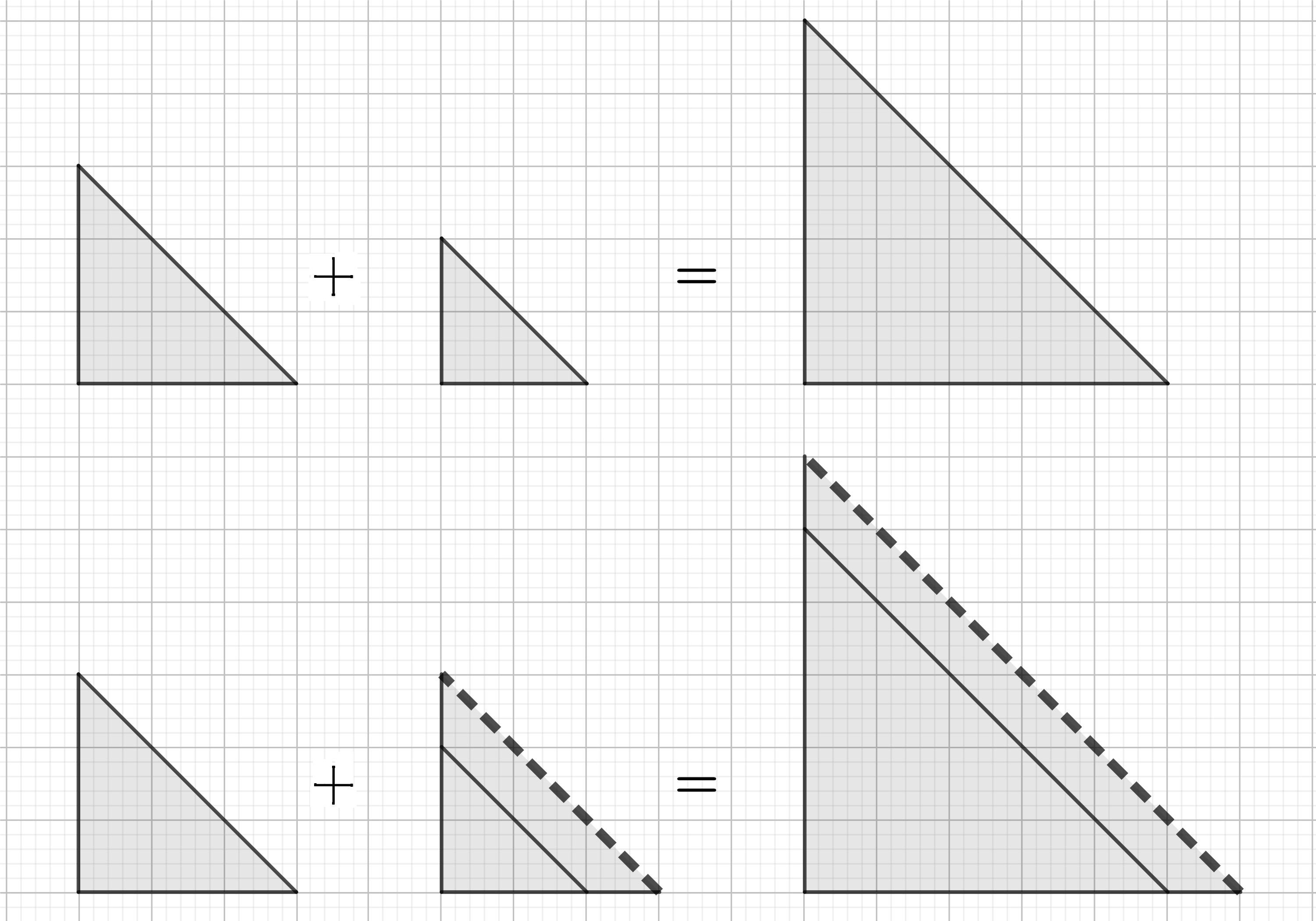
Figure 2. new face in $C$ and in $C+B$

In $\Omega_{2}$ we can consider $\delta\Omega$ in more detail. Note that it is located in the intersection of new rows and columns. Since all new conditions are concentrated in the common face we can group up all linear equations in $\delta\Omega$ and obtain single algebraic equation$\colon$

$$\delta c_{1}f^{\delta}_{1}+\delta c_{2}f^{\delta}_{2}=0$$

Where $f_{i}^{\delta}=f_{i}|_{d_{i}E(-1,-1)}$. We deduce that $(\delta c_{1},\delta c_{2})=\mu(f_{2}^{\delta},-f_{1}^{\delta})$, $\mu\in\mathbb{C}^{D_{1}E(-1,-1)\ominus d_{2}E(-1,-1)}\cap\mathbb{C}^{D_{2}E(-1,-1)\ominus d_{1}E(-1,-1)}$. If $D_{1}+d_{1}>D_{2}+d_{2}$ then coefficients of $\delta c_{1}$ will automatically vanish. So without loss of generality we assume that $D_{1}+d_{1}=D_{2}+d_{2}$. And thus $\mu\in\mathbb{C}^{D_{1}-d_{2}+1}=\mathbb{C}^{D_{2}-d_{1}+1}$.

For matrices of the form 4.2 we have $\operatorname{rk}\Omega_{2}\geq\operatorname{rk}\Omega_{1}+\operatorname{rk}\delta\Omega$. Thus, $\delta\operatorname{rk}\Omega=\operatorname{rk}\Omega_{2}-\operatorname{rk}\Omega_{1}\geq\operatorname{rk}\delta\Omega$ and $-\delta\operatorname{rk}\Omega\leq-\operatorname{rk}\delta\Omega$. We obtain, by the dimension theorem for vector spaces $\delta\dim V-\operatorname{rk}\delta\Omega=\dim\mathbb{C}^{D_{2}-d_{1}+1}$. We have computed all terms we needed. Finally, we substitute all data into the variation of $\delta\dim\mathcal{V}_{A}^{C,I}$

$$\delta\dim\mathcal{V}_{A}^{C,I}=\delta\dim V-\delta\operatorname{rk}\Omega-\delta\ker\phi\leq$$

$$\leq\delta\dim V-\operatorname{rk}\delta\Omega-\delta\ker\phi=$$

$$=D_{1}-d_{2}+2-(D_{1}-d_{2}+2)=0.$$

We can see that by increasing degrees of $C$ we make no affect on $\dim\mathcal{V}_{A}^{C,I}$. Without loss of generality assume that $d_{1}\leq d_{2}$. The minimal $(D_{1},D_{2})$ satisfying the property $D_{1}+d_{1}=D_{2}+d_{2}$ is $(d_{2}-d_{1},0)$. We take it as a foundation.

1. $d_{2}>d_{1}\geq 2$.

   Let us find all linear $l$ that can be represented in the form $l=c_{1}f_{1}+c_{2}f_{2}$, $c_{2}\in\mathbb{C}^{*}$. If we restrict the system to the face $E(-1,-1)$, as before, we obtain that $f_{2}|_{d_{2}E(-1,-1)}$ is divisible by $f_{1}|_{d_{1}E(-1,-1)}$. And this ends with a contradiction. So, in this case $\dim\mathcal{V}_{A}^{I}=0$.

2. $d_{2}>d_{1}=1$. In a similar way we obtain $l=cf_{1}$, $c\in\mathbb{C}$. So $\dim\mathcal{V}_{A}^{I}=1$

3. We easily obtain $\dim\mathcal{V}_{A}^{I}=2$.

In section 7 we will generalise this method to arbitrary dimension $n$ for $2$ bodies in the ring of Laurent polynomials.

5. Existence of a normal chain of a convex polytope.

In this section we prove the existence of a normal chain of a convex body. This will be useful in the next section. Let $X\subset\mathbb{R}^{n}$ be a convex polytope of maximal dimension with integral vertices. Let $L$ be the number of its faces. We can represent $X$ as a set of solutions of a system of $L$ inequalities $x.a_{i}\geq b_{i}$, $i\in\{1,\ldots,L\}$. If $h_{O}^{\epsilon}\colon\mathbb{R}^{n}\rightarrow\mathbb{R}^{n}$ is a fixed homothety with the center in $O$ and factor $\epsilon$, we will denote $h_{O}^{\epsilon}(X)$ by $\epsilon X$ for short. In the case when $O$ is the origin $\epsilon X$ can be represented in the form $x.a_{i}\geq\epsilon b_{i}$, $i\in\{1,\ldots,L\}$. In all proofs we assume that the center of homothety is always in the origin since it is more convenient for notation and computations. We denote by $E_{X}$ the set of all edges of $X$ enumerated in some order. We denote the length of $E$ by $l(E)$. Face with the normal vector $a_{i}$ is denoted by $F_{i}$ since in this section we do not deal with curves and this will not lead to confusion. We assume as was mentioned that $O\in\operatorname{int}(X)$.

         Definition 5.1.

We will say that the chain of convex polytopes

$$X\subset\epsilon_{0}X\subset X_{1}\subset X_{2}\subset\ldots\subset X_{kL+j}\subset\ldots$$

is normal if we have the following$\colon$

1. for $\epsilon_{0}>1$ we have $\mathbb{Z}(\epsilon_{0}X)=\mathbb{Z}(X)$.

2. for all $k\in\mathbb{N}$ we have $X_{kL}=\epsilon_{k}X$ for some $\epsilon_{k}>0$.

3. for all $j\in\{1,\ldots,L-1\}$ and for all $k\in\mathbb{N}$, $X_{kL+j}$ is given by the system

   $$\{x.a_{1}\geq\epsilon_{k+1}b_{1},\ldots,\ x.a_{j}\geq\epsilon_{k+1}b_{j},\ x.a_{j+1}\geq\epsilon_{k}b_{j+1},\ldots,\ x.a_{L-1}\geq\epsilon_{k}b_{L-1}\}$$

4. The number of faces of $X_{i}$ is $L$.

5. $\cup X_{i}=\mathbb{R}^{n}$.

6. for all $i$ we have $X_{i}=X+(X_{i}\ominus X)$.

7. For all $i$ we have $\mathbb{Z}(X_{i+1}\ominus X_{i})$ is either empty or lies in a hyperplane.

We would like to give some clarification. Except the second one, each term $X_{i}$ in the chain is derived from the previous one $X_{i-1}$ by shifting one of its faces. We require that such deformations do not change the set of faces of $X_{i-1}$, and when all faces are used, we end up with a pure homothety of $X$. In the next section we will see that normal chains are useful in proving that the term $\epsilon_{+}X$ is a foundation. To demonstrate what happens when we shift faces of a non-smooth polytope we consider the following example in dimension $3\colon$

         Example 5.2.

Take a square pyramid, depicted below (figure 3), as $C_{1}$, the same pyramid, with shifted face as $C_{2}$ and the homothety of $C_{1}$ with factor $1/2$ as $B$. Note that $C_{1}$ has a vertex attached to 4 faces at once. After the deformation, the set of edges will change. But, despite this, we still have $C_{2}=B+(C_{2}\ominus B)$. We will show that this situation is general.

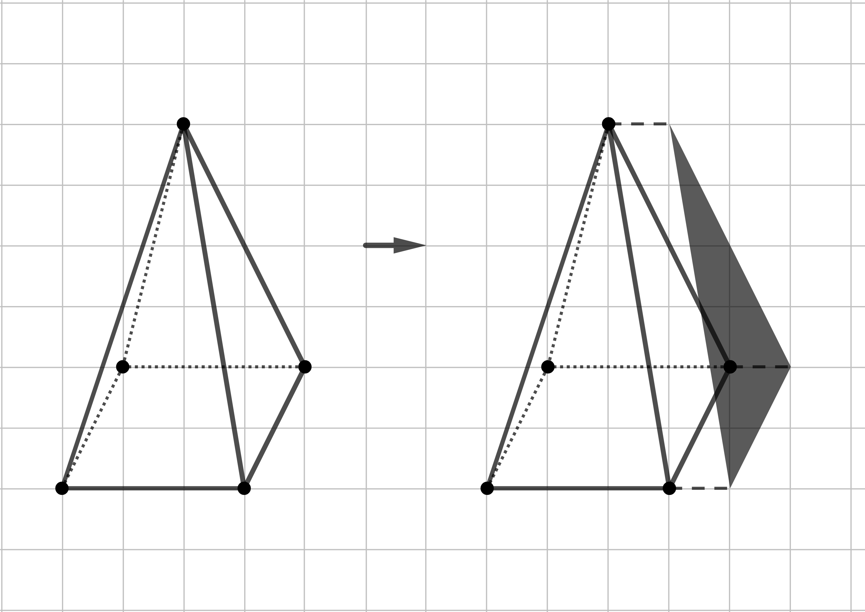
Figure 3. Deformation of non-smooth polytope

Now, we do some work to construct a normal chain for arbitrary $X$. We will say that $Y$ can be inserted into a normal chain that corresponds to $X$ if

$$X\subset\epsilon_{0}X\subset\ldots\subset Y$$

satisfies conditions (1)-(4) and (6) of definition 5.1 up to $Y$. Any inclusion in a normal chain will be called normal deformation with parameter $\epsilon$ at some face. We start here with the following lemma that allows us to build the first term of a normal chain$\colon$

         Lemma 5.3.

Let $X$ be an arbitrary polytope with integral vertices. Then there exists $\epsilon_{0}>1$ such that $\mathbb{Z}(\epsilon_{0}X)=X$.

Proof.

Consider the function

$$N\colon[1,\infty)\rightarrow\mathbb{N}$$

$$\epsilon\mapsto|\epsilon X\cap\mathbb{Z}^{n}|$$

It is clear that $t_{2}X\subset t_{1}X$ for $1<t_{2}<t_{1}$ thus $N(t_{1})\geq N(t_{2})$. We have two possible options

1. for all $\epsilon$ in some neighbourhood $U$ of $1$ we have $N(\epsilon)=|X\cap\mathbb{Z}^{n}|$

2. $N(1)=|X\cap\mathbb{Z}^{n}|$, but for any $\epsilon>1$ we have $N(\epsilon)>|X\cap\mathbb{Z}^{n}|$.

In the first case we can take any $\epsilon\in U\setminus 1$ and finish the proof. In the second case for any $t>1$ there exists a point $p(t)\in\mathbb{Z}^{n}$ such that $p(t)\in tX\setminus X$. We obtain a contradiction since there are only finite number of integral points in $tX\setminus X$ for any finite $t$. ∎

We give the following fact from linear agebra, we will use it only once in the lemma 5.5.

         Lemma 5.4.

Let $X\subset\mathbb{R}^{n}$ be a convex polytope. Let $u,v$ be its vertices and $u$ can be isolated from other vertices of $X$ by the linear map $\phi$, i.e. there exists $t\in\mathbb{R}$ s.t. $\phi.u<t<\phi.x$, for all vertices $x\in X$ except $u$. Then there exists a path $\Gamma$ from $u$ to $v$ consisting of edges of $X$ s.t. $\phi$ is monotone along $\Gamma$.

Proof.

Let $V$ be the set of all vertices of $X$. Since $v\in V$ we have $(v-u).\phi>0$. Assume that for all edges $e$ starting from $v$ w have $(e+v-u).\phi\geq(v-u).\phi$. Here we consider $e$ as a vector that connects two vertices. From $(e+v-u).\phi\geq(v-u).\phi$ we have $e.\phi\geq 0$ for all edges starting from $v$. Since $X$ lies in the cone spaned by all such $e$ we deduce that $\forall x\in X$, $x.\phi\geq v.\phi$. That contradicts with the property $u.\phi<v.\phi$. So we see that there exists at least one edge $E_{1}$ s.t. $(E_{1}+v-u).\phi<(v-u).\phi$. Since $E_{1}+v-u$ is also a vertex we can write $(E_{1}+v).\phi\geq u.\phi$, then, finally, we have, for some edge $E_{1}$ starting from $v\colon$

$$0\leq(E_{1}+v-u).\phi<(v-u).\phi$$

and the equality holds if and only if $E_{1}+v-u=0$. Since the set of all values $\{x.\phi|x\in V\}$ is discrete, for the finite number of steps we eventually get the representation $u=v+E_{1}+\ldots+E_{k}$ with the property $(v+E_{1}+\ldots+E_{i+1}).\phi<(v+E_{1}+\ldots+E_{i}).\phi$ and it proves the statement of the lemma. ∎

         Lemma 5.5.

Let $X_{0}=\epsilon_{0}X$ for some $X$. Let $X_{0}$ be given by the system of inequalities

(5.1) $$\{x.a_{1}\geq b_{1},\ldots,\ x.a_{j}\geq\ b_{j},\ x.a_{j+1}\geq b_{j+1},\ldots,\ x.a_{L}\geq b_{L}\}$$

Then for sufficiently small $\tau_{1},\ldots,\tau_{k}>0$ polytopes $X(\tau_{1},\ldots,\tau_{k})$ given by the system

(5.2) $$\{x.a_{1}\geq(1+\tau_{1})b_{1},\ldots,\ x.a_{k}\geq\ b_{k}(1+\tau_{k}),\ x.a_{k+1}\geq b_{k+1},\ldots,\ x.a_{L}\geq b_{L}\}$$

can be inserted into a normal chain $X(\tau)=X\subset\epsilon_{0}X\subset X(\tau_{1},0,\ldots,0))\ldots\subset X(\tau_{1},\tau_{2},\ldots,\tau_{k},0,\ldots,0)$.

Proof.

By assumption each edge $E\subset E_{{X_{0}}}$ of $X_{0}$ is given by the system of $n-1$ equations and $L-n+1$ inequalities from the system 5.1. Then, for sufficiently small $\tau=(\tau_{1},\ldots,\tau_{k})$ we have that new set of edges of $X(\tau)$ consists of two components$\colon$

1. Edges $E_{i}(\tau)$ parallel to the corresponding edges of $X$. And by continuity, their lengths are still longer than the corresponding edges of $X$ for sufficiently small $\tau$.

2. New edges $e^{0}_{j}(\tau)$ which have unknown directions. And their lengths are continuous functions of $\tau$ such that $e^{0}_{j}(0)=0$.

It remains to show that $X(\tau)=X+(X(\tau)\ominus X)$ for sufficiently small $\tau$. Let $V(\tau)$ be one of the vertices of $X(\tau)$. We have $V(0)=V_{0}$ for some vertex $V_{0}$ of $X_{0}$. Let $V_{X}$ be the corresponding vertex of $X$. We will show that $V(\tau)-V_{X}\in X(\tau)\ominus X$. Indeed, assume that $X+(V(\tau)-V_{X})\not\subset X(\tau)$. Then, there exists a vertex $x$ of $X$ such that $x+(V(\tau)-V_{X})\notin X_{0}$. By lemma 5.4 we can choose $\phi\in\mathbb{R}^{n}$ such that $\phi(x+(V(\tau)-V_{X}))>\phi(U(\tau))$, where $U(\tau)$ is a vertex of $X_{0}$ such that $U(0)$ corresponds to $x$ in $X_{0}$. And we can choose a path $E_{1},\ldots,E_{M}$ from $V(\tau)$ to $x+(V(\tau)-V_{X})$ such that $\phi(E_{i})>0$. Analogously, we can choose path from $V(\tau)$ to $U(\tau)$ consisting of $\lambda_{i}(\tau)E_{i}$ for some $\lambda_{i}(\tau)>1$ and of some additional edges $e^{0}_{j}(\tau)$. Let us substitute this data to $\phi(x+(V(\tau)-V_{X}))>\phi(U(\tau))$. We will obtain$\colon$

$$\sum(1-\lambda_{i}(\tau))\phi(E_{i})>\sum\phi(e^{0}_{j}(\tau)).$$

The left-hand side of the inequality tends to some negative number as $\tau\rightarrow+0$. And the right-hand side of it approaches zero. That means that there exists $T>0$ such that for all $\tau\in(0,T)$ we obtain a contradiction and $(V(\tau)-V_{X})\in X(\tau)\ominus X)$. By convexity, we have that $X(\tau)\ominus X$ is a convex hull of the set of all such $V(\tau_{0})-V_{X}$ for sufficiently small $\tau_{0}$ which is well defined since the set of all vertices is finite.

∎

From lemmata 5.3, 5.5 we know that for given $X$ we can define the chain of inclusions, satisfying all properties of the definition 5.1 except (2).

To construct a normal chain from the initial terms we need to adjust all $\tau_{i}$ to be of the same value. The next simple lemma allows us to do it$\colon$

         Lemma 5.6.

Let $f_{i}\colon\mathbb{R}^{M}\rightarrow\mathbb{R},\ i\in\{1,\ldots,\ L\},\ M\in\mathbb{N}$, be continuous functions such that $f_{i}(0)=T_{i}>0$. Then there exists $\tau>0$ such that $\forall\ i$ we have $\tau<f_{i}(\tau,\ldots,\ \tau)$.

Proof.

Let $T_{k}=\min T_{i}$. Since $f_{i}$ are continuous, for some neighbourhood $U$ of $0$ we have $T_{k}/2<f_{k}(x)\leq f_{i}(x)$ for all $x\in U$ and all $i$. Restrict $f_{i}$ on the diagonal and take any positive $\tau$ for which $(\tau,\ldots,\ \tau)\in U$. ∎

Finally we are ready to construct the first $L$ terms of the normal chain starting from $X$. Let us fix $\epsilon_{0}$ that satisfies the first condition of definition 5.1. By induction, we define the sequence of functions $\Theta_{i}(t_{1},\ldots,t_{i-1})$. Let $\Theta_{1}$ be the upper bound of all $t$ such that $X_{1}(t)$ defined above is a new term of the normal chain

$$X\subset\epsilon_{0}X\subset X_{1}(t)$$

Now, assume that $j$ terms of the chain is constructed

$$X\subset\epsilon_{0}X\subset X(t_{1})\subset\ldots\subset X(t_{1},\ldots,t_{k})$$

where we define $X(t_{1},\ldots,t_{k})$ just as we did in the proof of 5.5.

We define at this step $\Theta_{j+1}(t_{1},\ldots,\ t_{j})$ to be the upper bound of all $t$ such that

$$X\subset\epsilon_{0}X\subset X_{1}(t_{1})\subset\ldots\subset X_{j}(t_{1},\ldots,t_{j})\subset X_{j+1}(t_{1},\ldots,t_{j},t_{j+1})$$

satisfies all properties of normal chain except for (2) and (5) of course. As it was shown all $\Theta$ are well defined for any order of deformations and are continues in some neighbourhood of zero.

         Lemma 5.7.

For a given $X$ there exists $\tau>0$ such that

$$X\subset\epsilon_{0}X\subset X_{1}(\tau)\subset\ldots\subset X_{j}(\tau,\ldots,\tau)\subset\ldots\subset X_{L}(\tau,\ldots,\tau)=(1+\tau)\epsilon_{0}X.$$

Proof.

Apply 5.6 to the set of functions $\Theta_{i}$ for $i\in\{1,\ldots,\ L\}$. ∎

From the first $L$ terms we can easily deduce the entire chain.

         Lemma 5.8.

If we have the first $L$ terms of a normal chain, we can extend it to complete chain to infinity satisfying all properties of definition 5.1 except (7).

Proof.

Assume we have

$$X\subset\epsilon_{0}X\subset X_{1}\subset\ldots\subset\ldots\subset X_{L}=\epsilon\epsilon_{0}X.$$

for some $\epsilon>1$. Take $X_{L+i}=\epsilon X_{i}$. It is easy to see that this choice satisfies the definition. By induction we complete the entire chain. ∎

To complete the construction of a normal chain we need to satisfy the property (7). To make this possible we prove two more statements.

         Lemma 5.9.

If we have the fragment of length $L$ of a normal chain

$$\ldots\subset X_{kL+1}\subset\ldots\subset X_{(k+1)L}\subset$$

we can replace it with the fragment of length $2L$ with the same first and last terms

Proof.

Let $X_{(k+1)L}=\epsilon X_{kL}$. Pick some $1<\tilde{\epsilon}<\epsilon$. Since $\tilde{\epsilon}<\epsilon$ we can construct the fragment

$$\ldots\subset X_{kL+1}\subset\ldots\subset\tilde{\epsilon}X_{kL}\subset$$

as it was shown before in lemma 5.6. And by the same reasons since $\epsilon/\tilde{\epsilon}>1$ we can extend $\tilde{\epsilon}X_{kL}$ to $\epsilon X_{kL}$. ∎

         Lemma 5.10.

For a given $X$ we can construct a normal chain $X\subset X_{*}$ such that $\mathbb{Z}(X_{m+1})\setminus\mathbb{Z}(X_{m})$ is either empty or is contained in a hyperplane that is parallel to $F_{m+1}$.

Proof.

Since $\mathbb{Z}(X_{m+1})\setminus\mathbb{Z}(X_{m})$ is finite then by the previous lemma 5.9 for any chain $X\subset X_{*}$ we can find a refinement $X\subset\bar{X}_{*}$ so that $\mathbb{Z}(\bar{X}_{m+1})\setminus\mathbb{Z}(\bar{X}_{m})$ is either empty or lies in a hyperplane. ∎

6. Properties of $\ominus$ operation related to normal chains.

Assume that we have a normal chain $X\subset X_{*}$ corresponding to a convex polytope with integral vertices. Note that we do not require from elements of $X_{*}$ to have integral vertices because it is more convenient for us to have an option to deform $X_{*}$ in more continues way. The normal chains defined and developed in the previous section can have as small gap between successive terms as we want them to have by lemma 5.9. But of course, since $X_{*}$ are not integral in general we need some additional tools to use it in the proof of theorem 1.7. Because we will use the notion of normal chain to construct a chain of supports of some sequence of polynomials. Now, let us show some properties of $\ominus$ operation related to normal chains that will be important for work.

Just for simplicity of notation

         Definition 6.1.

Let $X\subset\ldots X_{m}\subset X_{m+1}\subset$ be normal chain starting from $X$. We will call $\alpha\in\mathbb{R}^{n}$ direction of deformation in inclusion $X_{m}\subset X_{m+1}$ if $\alpha$ is perpendicular to the face of deformation in this inclusion.

Normal chains behave well with $\ominus$ operation. To be precise$\colon$

         Lemma 6.2.

Let $X\subset\ldots\subset X_{m}\subset X_{m+1}\subset\ldots$ be a normal chain and $\alpha$ be the direction of deformation in the inclusion $X_{m}\subset X_{m+1}$. Then $(X_{m+1}\setminus X_{m})\ominus X(\alpha)=(X_{m+1}\ominus X)\setminus(X_{m}\ominus X)$.

Proof.

1. $\subset$ part$\colon$Let $x\in(X_{m+1}\setminus X_{m})\ominus X(\alpha)$. By definition $x+X\not\subset X_{m}$, so $x\notin X_{m}\ominus X$. Since $X_{m}\subset X_{m+1}$ is a normal deformation and $X_{m},\ X_{m+1}$ are elements of a normal chain by lemma 5.5 we deduce that each element of $(X_{m+1}\setminus X_{m})\ominus X(\alpha)$ can be extended to $X_{m+1}\ominus X$.

2. $\supset$ part$\colon$ Let $x\in(X_{m+1}\ominus X)\setminus(X_{m}\ominus X)$. If $x\in X_{m+1}\ominus X$ then $X(\alpha)+x\subset X_{m+1}$ and $x\in X_{m+1}\ominus X(\alpha)$. Assume that $x+X(\alpha)\cap X_{m}$ then either $x+X(\alpha)\subset X_{m}$ which is impossible or $x\in X_{m}(\alpha)\ominus X(\alpha)$ then by lemma 5.5 we have $x\in X_{m}\ominus X$ again. Both alternatives give contradiction.

∎

To prove the main result of the next section we must make the final preparatory steps. In general, elements of $C$ will not be integral polytopes, but we are going to use them as supports for some polynomial equations. To do this we prove the following formula$\colon$

         Lemma 6.3.

Let $X\subset\mathbb{Z}^{n}$ be a convex polytope and $X_{m}\subset X_{m+1}$ be like in the lemma 6.2. Then $\mathbb{Z}((X_{m+1}\ominus X)\setminus(X_{m}\ominus X))=\mathbb{Z}(X_{m+1}\setminus X_{m})\ominus X(\alpha)$.

Proof.

By lemma 6.2 we have $(X_{m+1}\setminus X_{m})\ominus X(\alpha)=(X_{m+1}\ominus X)\setminus(X_{m}\ominus X)$. From this we tautologically obtain

$$\mathbb{Z}((X_{m+1}\ominus X)\setminus(X_{m}\ominus X))=\mathbb{Z}((X_{m+1}\setminus X_{m})\ominus X(\alpha))$$

We are going to show that $\mathbb{Z}((X_{m+1}\setminus X_{m})\ominus X(\alpha))=\mathbb{Z}(X_{m+1}\setminus X_{m})\ominus X(\alpha)$. Let $Y\subset\mathbb{R}^{n}$ be a convex subset and $B\subset\mathbb{Z}^{n}$ also be convex. Then $\mathbb{Z}(Y\ominus B)=\mathbb{Z}(Y)\ominus B$.

1. $\subset$ part$\colon$ Let $x\in\mathbb{Z}(Y\ominus B)$ then $x\in\mathbb{Z}^{n},\ x+B\subset Y$. Assume that $x+B\not\subset\mathbb{Z}(Y)$. That means we have a vertex $x+y\notin\mathbb{Z}(Y)$. But $x+y\in\mathbb{Z}^{n}$ and if $x+y\in Y$ then $x+y\in\mathbb{Z}(Y)$.

2. $\supset$ part$\colon$ Let $x\in\mathbb{Z}(Y)\ominus B$ then $x+B\subset\mathbb{Z}(Y)\subset Y$ and $x\in\mathbb{Z}(Y\ominus B)$.

Finally, we apply this formula to the case $Y=X_{m+1}\setminus X_{m}$ and $B=X(\alpha)$. ∎

Condition for $X$ to have integral vertices is important. See figure 4.

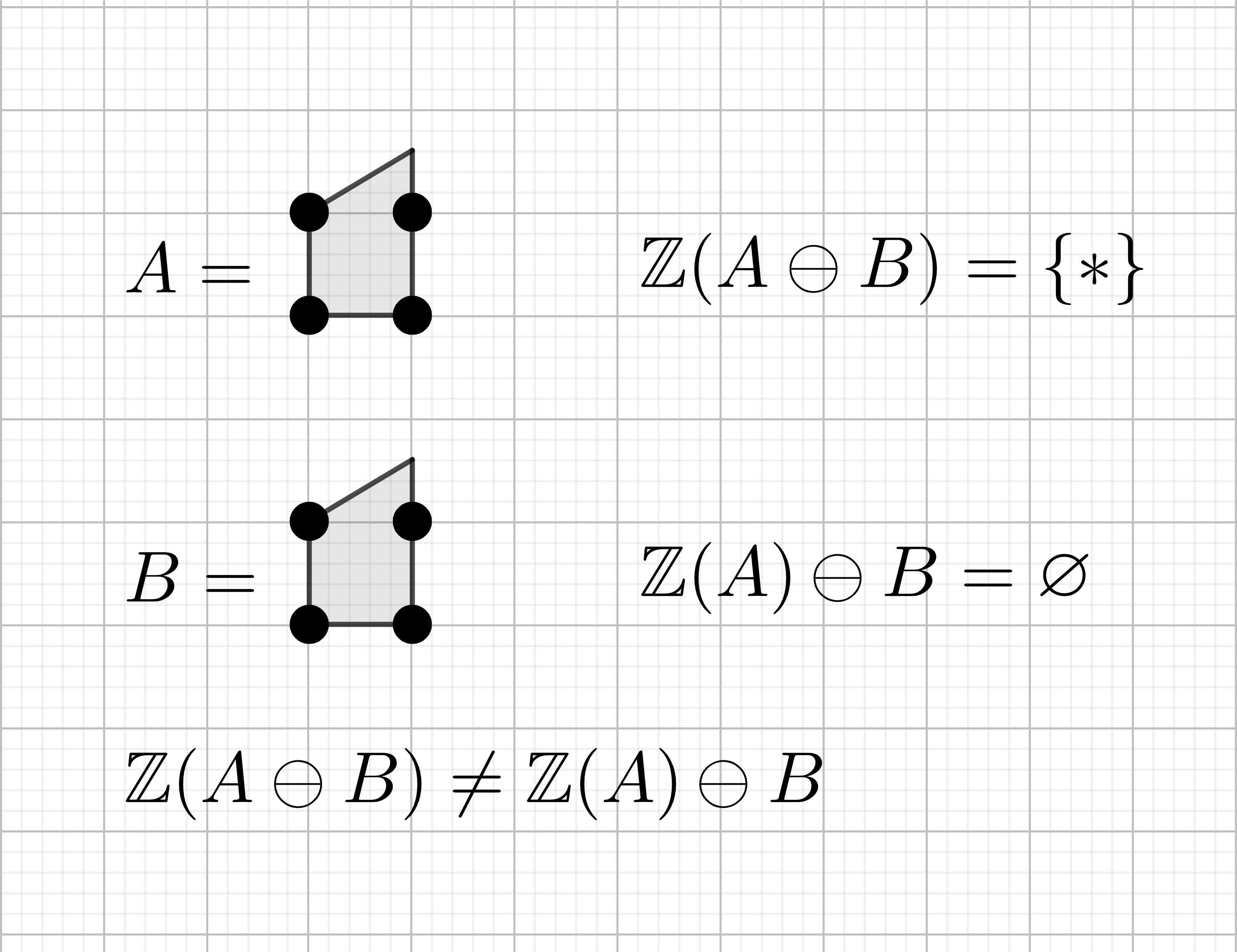
Figure 4. example that shows why $X$ must be integral

         Lemma 6.4.

Let $X\subset\mathbb{Z}^{n}$ be a convex polytope. Let $X\subset\ldots\subset X_{m}\subset X_{m+1}\subset\ldots$ be a normal chain. Then $\mathbb{Z}(X_{m+1}\ominus X)\setminus\mathbb{Z}(X_{m}\ominus X)=\mathbb{Z}((X_{m+1}\ominus X)\setminus(X_{m}\ominus X))$. Also, we have $\mathbb{Z}(X_{m}\ominus X)\subset\mathbb{Z}(X_{m+1}\ominus X)$.

Proof.

1. $\subset$ part$\colon$ Let $x\in\mathbb{Z}(X_{m+1}\ominus X)\setminus\mathbb{Z}(X_{m}\ominus X)\Rightarrow x\in X_{m+1}\ominus X,\ x\in\mathbb{Z}^{n}$. Assume that $x\in X_{m}\ominus X$, then $x\in\mathbb{Z}(X_{m}\ominus X)$ since $x$ is integral. This is not possible. We deduce that $x\in(X_{m+1}\ominus)\setminus(X_{m}\ominus X)$. Since $x\in\mathbb{Z}^{n}$ we conclude that $x\in\mathbb{Z}((X_{m+1}\ominus X)\setminus(X_{m}\ominus X))$.

2. $\supset$ part$\colon$ Let $x\in\mathbb{Z}((X_{m+1}\ominus X)\setminus(X_{m}\ominus X))\Rightarrow x\in\mathbb{Z}^{n},\ x+X\subset X_{m+1},x+X\not\subset X_{m}$. Thus, $x\in\mathbb{Z}(X_{m+1}\ominus X)$. Assume that $x\in\mathbb{Z}(X_{m}\ominus X)=\mathbb{Z}(X_{m})\ominus X$. Then $x+X\subset\mathbb{Z}(X_{m})\subset X_{m}$. Contradiction.

For the second part, consider $x+X\subset X_{m}\subset X_{m+1}\Rightarrow X_{m}\ominus X\subset X_{m+1}\ominus X\Rightarrow\mathbb{Z}(X_{m}\ominus X)\subset\mathbb{Z}(X_{m+1}\ominus X)$. ∎

7. Computing $\dim\mathcal{V}^{B}_{A}$ in dimension $n$ for $2$ copies of $B$.

We dedicate this section to the proof of theorem 1.7. We will use widely all the material we have collected in two previous purely technical sections.

         Theorem 7.1.

Let $(A,B)$ be a pair of convex polytopes in $\mathbb{Z}^{n}$ such that $B$ is not a segment. Let $t\in{R}$ be such that $A\subset\mathbb{Z}((t+1)B)$. Then $(tB,tB)$ is a foundation for $(A,B,B)$.

Let $C=(C_{1},\ldots,C_{k})$, $\mathbb{C}^{C}=\mathbb{C}^{C_{1}}\oplus\ldots\oplus\mathbb{C}^{C_{k}}$ As in the example 4 we define the following map$\colon$

$$\phi^{C}\colon\mathbb{C}^{C}\rightarrow\mathbb{C}[\bf{x}]$$

$$(c_{1},\ldots,c_{k})\mapsto c_{1}f_{1}+\ldots+c_{k}f_{k}$$

In the space $\mathbb{C}^{C}$ we define a subspace $W_{A}^{C}$ by the condition $\operatorname{supp}(c_{1}f_{1}+\ldots+c_{k}f_{k})\subset A$. In this notation we have

$$\dim\mathcal{V}_{A}^{C,B}=\dim W_{A}^{C}-\dim\ker\phi^{C}$$

Now, choose $C$ as in the theorem 1.7. To show that $C$ is a foundation we will construct the chain of bodies such that

1. $\cup C_{i}=\mathbb{R}^{n}$

2. for each $i$, $\dim\mathcal{V}^{C_{i+1},B}_{A}-\dim\mathcal{V}^{C_{i},B}_{A}=\delta\dim W^{C_{i}}_{A}-\delta\ker\phi^{C_{i}=}0$

Take a normal chain $C_{*}$ starting from $B$. We start consideration from the least term $C_{i}$ in $C_{*}$ satisfying the property $A\subset\mathbb{Z}(C_{i}+B)$. We will show such chain satisfies the require properties. Denote $C_{i+1}\setminus C_{i}$ by $\delta C_{i}$ and $\dim\mathcal{V}_{A}^{B.C_{i+1}}-\dim\mathcal{V}_{A}^{B.C_{i}}$ by $\delta D_{i}$. First, we compute $\dim\ker\phi^{C_{i}}$.

         Lemma 7.2.

In the above notation, $\dim\ker\phi^{C_{i}}=|\mathbb{Z}(C_{i})\ominus B|$.

Proof.

For generic $(f_{1},f_{2})$ from $c_{1}f_{1}+c_{2}f_{2}=0$ we obtain $(c_{1},\ c_{2})=\mu(f_{2},\ -f_{1})$ where $\mu\in\mathbb{C}^{\mathbb{Z}(C_{i})\ominus B}$. ∎

The next lemma shows us that actually $\dim W_{A}^{C}$ cannot change to fast across the normal chain. That is why we use them.

         Lemma 7.3.

If $C_{i}\subset C_{i+1}$ is an inclusion in normal chain such that $A\subset\mathbb{Z}(C_{i}+B)$ then

$$\delta\dim W^{C_{i}}_{A}\leq|\mathbb{Z}(\delta C_{i})\ominus B(\alpha)|.$$

where $\alpha$ is the direction of deformation in the inclusion $C_{i}\subset C_{i+1}$.

Proof.

Let $W_{A}^{C_{i}}$ be defined by the system $\Omega_{i}$ of linear equations such that we enumerate columns of $\Omega_{i}$ by points of $\mathbb{Z}(C_{i})$ and rows by linear conditions obtained from the property that $c_{1}f_{1}+c_{2}f_{2}$ has no monomials outside $A$. We use similar notation for $\Omega_{i+1}$. Under this agreement we can see that $\Omega_{i+1}$ has the following form$\colon$

(7.1) $$\Omega_{i+1}=\left[\begin{array}[]{c|c c}\Omega_{i}&*\\ \hline\cr 0&\delta\Omega\end{array}\right]$$

where $\delta\Omega$ is the matrix in the intersection of new points in $\mathbb{Z}(C_{i+1})$ and new conditions given by new monomials in $(c_{1}+\delta c_{1})f_{1}+(c_{2}+\delta c_{2})f_{2}$. Since all the new monomials lie in the same plane $\mathbb{Z}(\delta C_{i})$ we can group them up. After this we obtain a single algebraic equation$\colon$

$$c_{1}|_{\mathbb{Z}(\delta C_{i})}f_{1}|_{B(\alpha)}+c_{2}|_{\mathbb{Z}(\delta C_{i})}f_{2}|_{B(\alpha)}=0$$

We deduce from it that

$$(\delta c_{1},\delta c_{2})=\lambda(f_{2}|_{B(\alpha)},\ -f_{1}|_{B(\alpha)})$$

where

$$\lambda\in\mathbb{C}^{\mathbb{Z}(\delta C_{i})\ominus B(\alpha)}.$$

By the dimension theorem from linear algebra we have

$$2|\mathbb{Z}(\delta C_{i})|-\operatorname{rk}\delta\Omega=\mathbb{Z}(\delta C_{i})\ominus B(\alpha).$$

By the inequality $\operatorname{rk}\Omega_{i+1}\geq\operatorname{rk}\Omega_{i}+\operatorname{rk}\delta\Omega$ we have $\delta\operatorname{rk}\Omega_{i}=\operatorname{rk}\Omega_{i+1}-\operatorname{rk}\Omega_{i}\geq\operatorname{rk}\delta\Omega$. and finally we have

$$\delta\dim W^{C_{i}}_{A}=2|\mathbb{Z}(\delta C_{i})|-\delta\operatorname{rk}\Omega_{i}\leq 2|\mathbb{Z}(\delta C_{i})|-\operatorname{rk}\delta\Omega=$$

$$=\mathbb{Z}(\delta C_{i})\ominus B(\alpha).$$

∎

         Theorem 7.4.

Let $A\subset\mathbb{Z}^{n}$. Let $C_{*}=\{B\subset C^{0}_{1}\subset C^{0}_{2}\subset\ldots\subset C^{0}_{N}\subset\ldots\}$ be a normal chain s.t. $A\subset\mathbb{Z}(B+C^{0}_{1})$. We denote $(\mathbb{Z}(C^{0}_{i}),\mathbb{Z}(C^{0}_{i}))$ by $C_{i}$. Then, we have $\dim\mathcal{V}_{A}^{B.C_{i}}=\dim\mathcal{V}_{A}^{B.C_{1}}=\dim\mathcal{V}_{A}^{B}$ for all $i\in\mathbb{N}$.

Proof.

By lemma 5.10 $C_{*}$ can be refined such that $\mathbb{Z}(\delta C_{i})$ is lying in a hyperplane parallel to $F_{j}$ for some $j\in\{1,\ldots,\ L\}$. Let $\alpha$ be the direction of deformation in the inclusion $C_{i}^{0}\subset C_{i+1}^{0}$. By lemma 7.3 we have

(7.2) $$\delta D_{i}=\dim\mathcal{V}_{A}^{B.C_{i+1}}-\dim\mathcal{V}_{A}^{B.C_{i}}\leq|\mathbb{Z}(\delta C_{i})\ominus B(\alpha)|-\delta\dim\ker\phi^{C_{i}}.$$

by the formula obtained in lemma 7.2 we have

$$\delta\dim\ker\phi^{C_{i}}=|\mathbb{Z}(C_{i+1})\ominus B|-|\mathbb{Z}(C_{i})\ominus B|=|\mathbb{Z}(C_{i+1}\ominus B)|-|\mathbb{Z}(C_{i}\ominus B)|.$$

The second equality is from 6.3. If $|\mathbb{Z}(C_{i+1})|=|\mathbb{Z}(C_{i})|$ then we obviously have $\delta D_{i}=0$. Otherwise,

$$|\mathbb{Z}(C_{i+1}\ominus B)|-|\mathbb{Z}(C_{i}\ominus B)|=|\mathbb{Z}((C_{i+1}\ominus B)\setminus(C_{i}\ominus B))|$$

by lemma 6.4. By lemma 6.3

$$\mathbb{Z}((C_{i+1}\ominus B)\setminus(C_{i}\ominus B))=\mathbb{Z}(\delta C_{i}\ominus B(\alpha))=\mathbb{Z}(\delta C_{i})\ominus B(\alpha).$$

We get $\delta\dim\ker\phi^{C_{i}}=\mathbb{Z}(\delta C_{i})\ominus B(\alpha)$. And $0\leq\delta D_{i}\leq|\mathbb{Z}(\delta C_{i})\ominus B(\alpha)|-|\mathbb{Z}(\delta C_{i})\ominus B(\alpha)|=0$. We conclude that $\delta D_{i}=0$ for all $i$ in the normal chain. ∎

Proof.

(Of theorem 1.7)

Take $v\in\mathbb{Z}^{n}$ and $t$ such that $A+v\subset\mathbb{Z}((t+1)B)$. We can extend the inclusion $B\subset tB)$ to a normal chain. Then, by theorem 7.4 $tB$ is a foundation. ∎

We now use the same technique to prove theorem 1.8.

Proof.

(Of theorem 1.8)

First note that in the same setting we can construct the negative normal chain using the same technique as we did in section 5. It will satisfy properties (2)-(4) and all edges of $C_{i}$ are shorter than the corresponding edges of $B$.

$$\ldots C_{-i-1}\subset C_{-i}\subset\ldots\subset\epsilon_{-1}B\subset B_{-{L}}\subset\ldots\subset B_{-1}\subset B$$

Here $\epsilon_{-1}$ satisfies $\mathbb{Z}(\epsilon_{-1}B)\subset\operatorname{int}(B)$ and there are no integral points between $\epsilon_{-}B$ and the boundary of $B$. To estimate $\dim\mathcal{V}_{A}^{B}$ let us consider $(A,B,B)$ as in the condition of theorem 1.8. For some $C_{-i}$ we can see that $A+v\subset C_{-i}+B$ for some integral $v$ and we can apply formula for $\delta\dim\mathcal{V}_{A}^{C,B}$. But, all terms in equation 7.2 tautologically vanish since for any face $F^{B}$ of $B$ and corresponding face $F^{C}$ of $C$ we have $F^{C}\ominus F^{B}=\varnothing$ for $C\subset\epsilon_{-1}B$. Consider the last fragment of negative normal chain of length $L$. This is the only place where $F^{B_{-i}}_{j}\ominus F^{B}_{j}$ might not be zero for some $i$ and some face $F_{j}$.

We enumerate $B_{-i}$ by its direction of deformation. We can shift faces of $B_{-i}$ to the faces of $B$ in any order. Note that $F_{i}^{B_{-i}}\ominus F_{i}^{B}\neq\varnothing$ if and only if all faces conjugated to $F_{i}$ are already shifted. We can choose the order of deformations such that there is only one face (obviously the final) for which $F^{B}_{-1}\ominus F^{B}=\{*\}$. But on the final step we have $\delta\dim\ker\phi$=1. And we conclude that $\delta\dim\mathcal{V}_{A}^{B}=0$. Let us show why we can do this, i.e. why such order of faces exists.

Consider the graph $\Gamma_{B}$ whose vertices are faces of $B$ and two vertices are connected by an edge if and only if the corresponding faces conjugate. We can locate vertices of $\Gamma_{B}$ in the corresponding vertices of dual polytope of $B$. Now, we define an order $R_{\psi}$ on $\Gamma_{B}$ by applying a linear form $\psi\in\mathbb{R}^{n}$. We will say that $v\geq u$ of $\Gamma_{B}$ if and only if $\psi(v)\geq\psi(u)$. Let us pick $\psi$ such that all $\psi(v)$ are distinct for all $v\in\Gamma_{B}$. For this $\psi$ let us shift faces in order $R_{\psi}$. It is easy to see that a face $F_{v}$ of $B$ is surrounded by shifted faces if and only if for all neighbours $u_{i}$ of the corresponding vertex $v$ we have $\psi(u_{i})<\psi(v)$. But for given order it is possible only for the final vertex, i.e. the final face of $B$.

∎

Combining theorems 1.7 and 1.8 we obtain 1.9.

8. Inequality involving Minkowski sum and $\ominus$ operation.

         Theorem 8.1.

In dimension $2$ for any convex polytopes we have the inequality $|A+B|+|A\ominus B|\geq 2|A|$.

Proof.

For any two non equal bodies $A,B$ we have $A\ominus B=\emptyset$ or $B\ominus A=\emptyset$. We consider the non-trivial case. Also, we assume that both $A,B$ are full dimensional. The initial inequality is equivalent to the following$\colon$

$$|A+B|-|A|-1\geq|A|-|A\ominus B|-1$$

Since we have $\operatorname{MV}(A,B)\geq r.h.s.$ by [24], it is sufficient to prove $l.h.s.\geq\operatorname{MV}(A,B)$. We use Pick’s formula and write$\colon$

$$\operatorname{MV}(A,B)=V(A+B)-V(A)-V(B)$$

$$V(A+B)=i(A+B)+|\delta(A+B)|/2-1$$

$$V(A)=i(A)+|\delta A|/2-1,$$

$$V(B)=i(B)+|\delta B|/2-1,$$

Consider the difference

$$|A+B|-|A|-1-\operatorname{MV}(A,B)=$$

$$=|A+B|-|A|-1-V(A+B)+V(A)+V(B)=$$

$$=i(A+B)+|\delta(A+B)|-i(A)-|\delta A|-1-i(A+B)-|\delta(A+B)|/2+1+i(A)+|\delta A|/2-1+i(B)+|\delta B|/2-1=$$

$$=|\delta(A+B)|/2-i(A)-|\delta A|-1+1+i(A)+|\delta A|/2-1+i(B)+|\delta B|/2-1=$$

$$=|\delta(A+B)|/2-|\delta A|/2+|\delta B|/2+i(B)-2$$

Since $|\delta B|/2\geq 3/2$, we should find all pairs $A,B$ s.t. $|\delta(A+B)|=|\delta A|,i(B)=0$ to conclude the proof. It’s easy to see that it is possible only in the case $B=\{pt\}$. Indeed, each edge of $A$ is represented in the boundary of $A+B$. Consider three cases$\colon$

1. There exist two parallel edges $E_{A}\subset\delta A$ and $E_{B}\subset\delta B$, that are corresponding to the same principal direction $\phi$. In this case, the boundary of $A+B$ would have an edge that is equal to the sum $E_{A}+E_{B}$. Then, $|\delta(A+B)|\geq|\delta A|-|E_{A}|+|E_{A}+E_{B}|=|\delta A|-|E_{A}|+|E_{A}|+|E_{B}|-1=|\delta|+|E_{B}|-1\geq|\delta A|+2-1=|\delta A|+1$.

2. There exist two adjacent edges $E_{1},E_{2}$ of $A$ and two vertices $p,q$ of $B$ s.t. $(E_{1}+p)\cap(E_{2}+q)=\varnothing$ and $E_{1}+p$, $E_{2}+q$ lie on the boundary of $\delta(A+B)$. In this case we have $|\delta(A+B)|\geq|\delta A|-(|E_{1}|+|E_{2}|-1)+(|E_{1}|+|E_{2}|)=|\delta A|+1$.

3. In the last case, all adjacent edges of $A$ are still being adjacent in $A+B$ and thus $|A+B|=|A|\Rightarrow B=\{pt\}$.

∎

         Conjecture 8.2.

The inequality written above also holds in dimension $\geq 3$.

References

- [1] W. D. Brownawell, Bounds for the degrees in the Nullstellensatz, Ann. Math. 126 (1987), 577–591.
- [2] Kollar, J., Sharp effective Nullstellensatz Journal of the American Mathematical Society 1 (1988): 963–75.
- [3] Canny, J., and I. Z. Emiris. A subdivision-based algorithm for the sparse resultant Journal of the Association for Computing Machinery 47 (2000): 417–51.
- [4] Carlos D’Andrea, Gabriela Jeronimo. Sparse Nullstellensatz, resultants and determinants of complexes. https://arxiv.org/abs/2407.13450v1
- [5] Frédéric Bihan, Alicia Dickenstein, Jens Forsgård. Sparse systems with high local multiplicity. https://arxiv.org/abs/2402.08410
- [6] Sabia, J., Solernó, P. Bounds for traces in complete intersections and degrees in the Nullstellensatz. AAECC 6, 353–376 (1995). https://doi.org/10.1007/BF01198015
- [7] M. Sombra, A sparse effective Nullstellensatz. Adv. in Appl. Math. 22 (1999), no. 2, 271–295.
- [8] Jan Tuitman, A Refinement of a Mixed Sparse Effective Nullstellensatz. International Mathematics Research Notices, Volume 2011, Issue 7, 2011, Pages 1560–1572, https://doi.org/10.1093/imrn/rnq127
- [9] D. N. Bernstein, The number of roots of a system of equations. Funct. Anal. Appl. 9 (1975), no. 3, 183–185.
- [10] M. Kapranov I.Gelfand and A. Zelevinsky, Discriminants, resultants and multidi- mensional determinants. 79(485):439–440, 1995.
- [11] A. Esterov, Galois theory for general systems of polynomial equations. Compositio Mathematica, 155(2):229–245, 2019
- [12] A. Esterov, Newton Polyhedra of Discriminants of Projections. Discrete Comput Geom 44, 96–148 (2010). https://doi.org/10.1007/s00454-010-9242-7
- [13] Cattani, E., Cueto, M.A., Dickenstein, A. et al. Mixed discriminants. Math. Z. 274, 761–778 (2013). https://doi.org/10.1007/s00209-012-1095-8
- [14] C. Borger and B. Nill, On defectivity of families of full-dimensional point configurations, Proc. Amer. Math. Soc. Ser. B 7, Volume, 43-51 (2020)
- [15] A. Gabrielov and A. Khovanskii, Multiplicity of a noetherian intersection. Providence, RI: American Mathe-matical Society, pages 119–130, 1998
- [16] A. Khovanskii, Newton polytopes and irreducible components of complete intersections. Izv. Math. 80 263, 2016
- [17] Dickenstein, Alicia, Sandra Di Rocco and Ralph Morrison. Iterated and mixed discriminants. (2021).
- [18] Jelonek, Z. On the effective Nullstellensatz. Invent. math. 162, 1–17 (2005). https://doi.org/10.1007/s00222-004-0434-8
- [19] A. G. Khovanskii, Newton polyhedra and toroidal varieties, Functional. Anal. i Prilozhen., 11:4 (1977), 56–64; Funct. Anal. Appl., 11:4 (1977), 289–296
- [20] D. Eisenbud, Commutative Algebra: With a View toward Algebraic Geometry, Grad. Texts in Math. 150, Springer, New York, 1995.
- [21] Miranda, Rick. Algebraic Curves and Riemann Surfaces. (1995).
- [22] Wulcan, E. Sparse effective membership problems via residue currents. Math. Ann. 350, 661–682 (2011). https://doi.org/10.1007/s00208-010-0575-6
- [23] W. Castryck, J. Denef F. Vercauteren: Computing zeta functions of nondegenerate curves, IMRP Int. Math. Res. Pap. 2006, Art. ID 72017, 57 pp.
- [24] I. Nikitin, Bivariate systems of polynomial equations with roots of high multiplicity. // Journal of Algebra and Its Applications, (2021); doi:10.1142/S0219498823500147
- [25] Weibel, C. (1994). An Introduction to Homological Algebra (Cambridge Studies in Advanced Mathematics). Cambridge: Cambridge University Press. doi:10.1017/CBO9781139644136