Half grid diagrams and Thompson links
Abstract
We define half grid diagrams and prove every link is half grid presentable by constructing a canonical half grid pair (which gives rise to a grid diagram of some special type) associated with an element in the oriented Thompson group. We show that this half grid construction is equivalent to Jones’ construction of oriented Thompson links in [6]. Using this equivalence, we relate the (oriented) Thompson index to several classical topological link invariants, and give both the lower and upper bounds of the maximal Thurston-Bennequin number of a knot in terms of the oriented Thompson index. Moreover, we give a one-to-one correspondence between half grid diagrams and elements in symmetric groups and give a new description of link group using two elements in a symmetric group.
1 Introduction
Grid diagrams have many interesting applications to knot theory and low dimensional topology (for example, relation to Legendrian and transverse knots [10]), and they provide a combinatorial way to compute some knot invariants such as knot Floer homology [9] and Khovanov homology [4]. In recent years, there have been plenty of studies about slicing a “closed” object into two or more “bordered” objects to obtain information from pieces, including bordered Heegaard Floer homology [8], bordered knot Floer homology [12], [13], and bordered Khovanov homology [15], [16]. It is well-known that every link has a grid diagram representing it, so slicing a link can be realized by slicing a grid diagram.
It is natural to ask what a “good” bordered grid diagram could be and whether we can split grid diagrams and get information from pieces. To answer these questions, let’s first recall some definitions related to grid diagrams.
Definition 1.1.
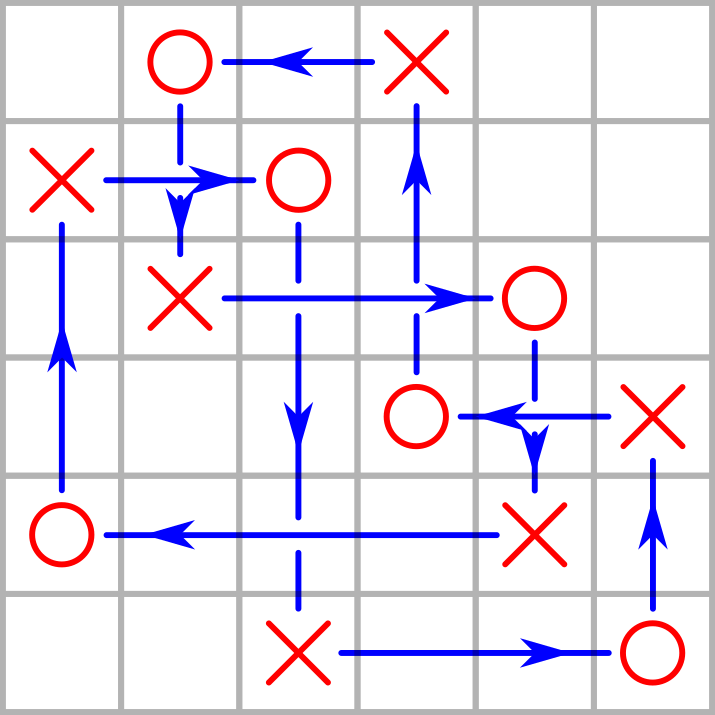
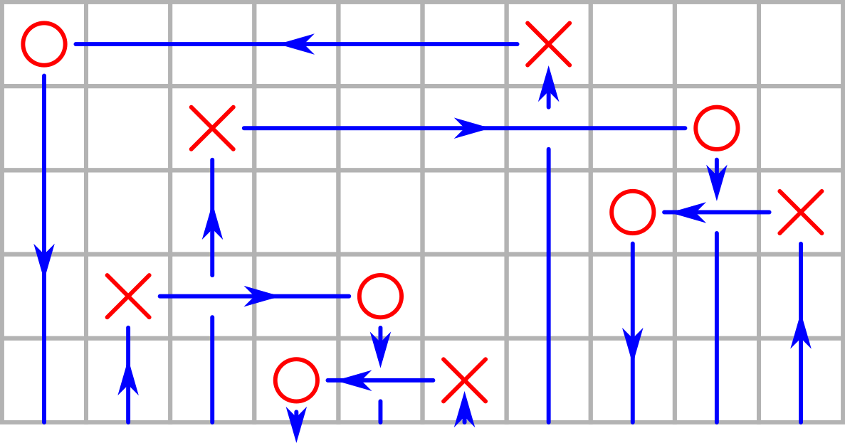
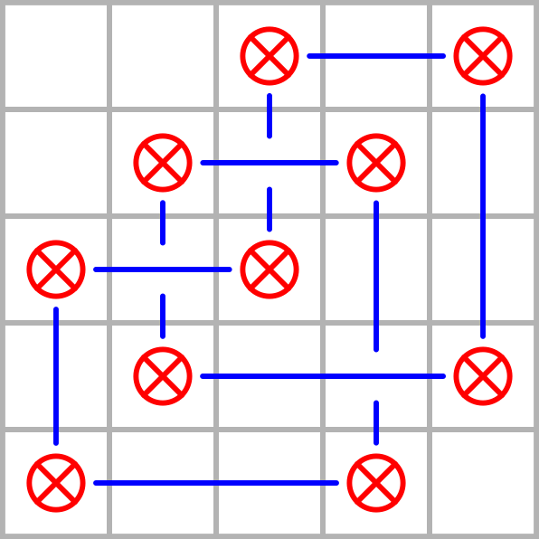
A grid diagram is an grid of squares, each of which is either empty or contains an or an . We require that in each row and column there are exactly two nonempty squares, one containing an and the other containing an .
Any grid diagram has an associated link defined as follows.
Definition 1.2.
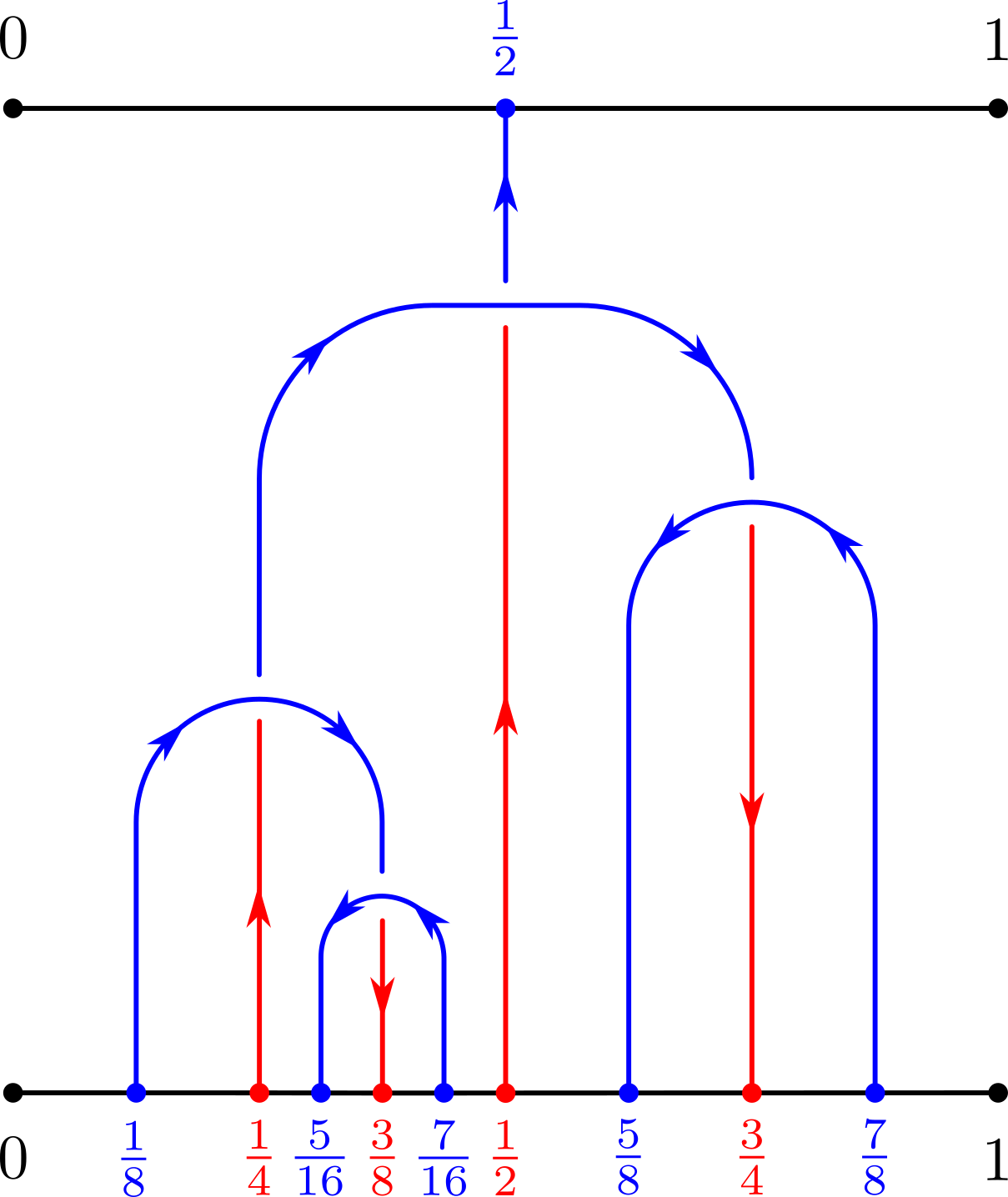
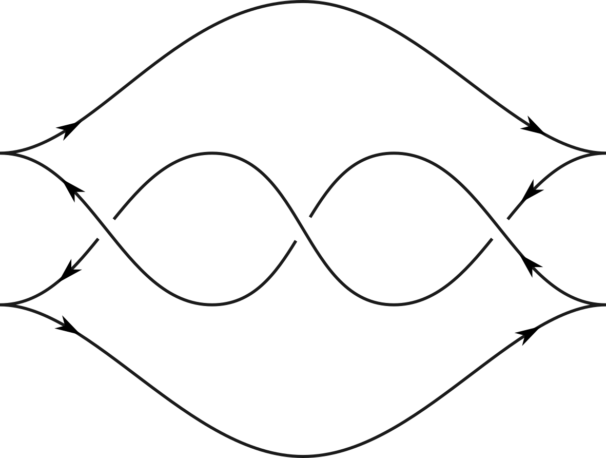
Let be an grid diagram. The oriented link associated to is obtained by connecting to in each row and connecting to in each column such that horizontal segments are always above vertical segments.
See Figure 1(a) for an example of a grid diagram and its associated link.
Remark 1.3.
The orientation and crossing conventions we are using on paper are slightly different from the usual conventions in [9]. The usual orientation convention is to connect to in each row and connect to in each column, with the crossing convention that vertical segments are always above horizontal segments. However, if we rotate a grid diagram with an associated link in our conventions by 90 degrees, it will become a grid diagram with an associated link in the usual conventions. The reason for using our conventions is to make the over and under crossing compatible with the ones from Thompson links (Section 3.1).
We now define half grid diagrams, which give rise to oriented tangles.
Definition 1.4.
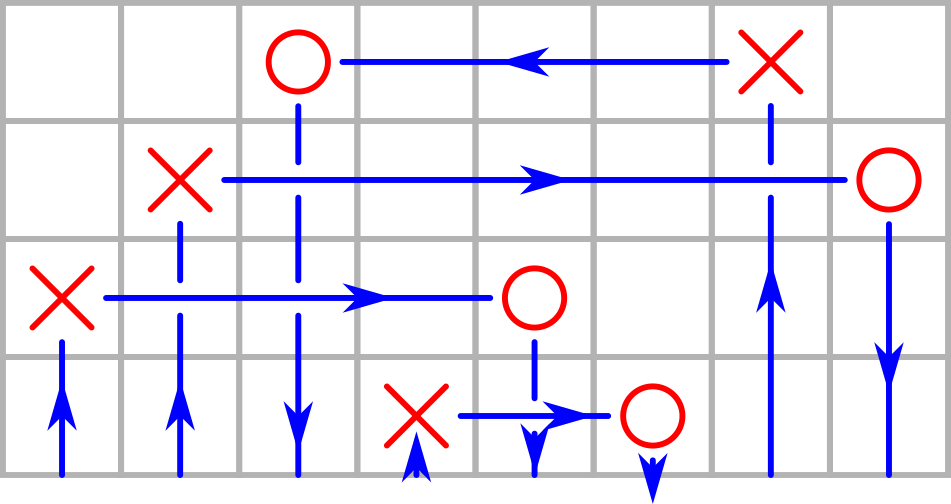
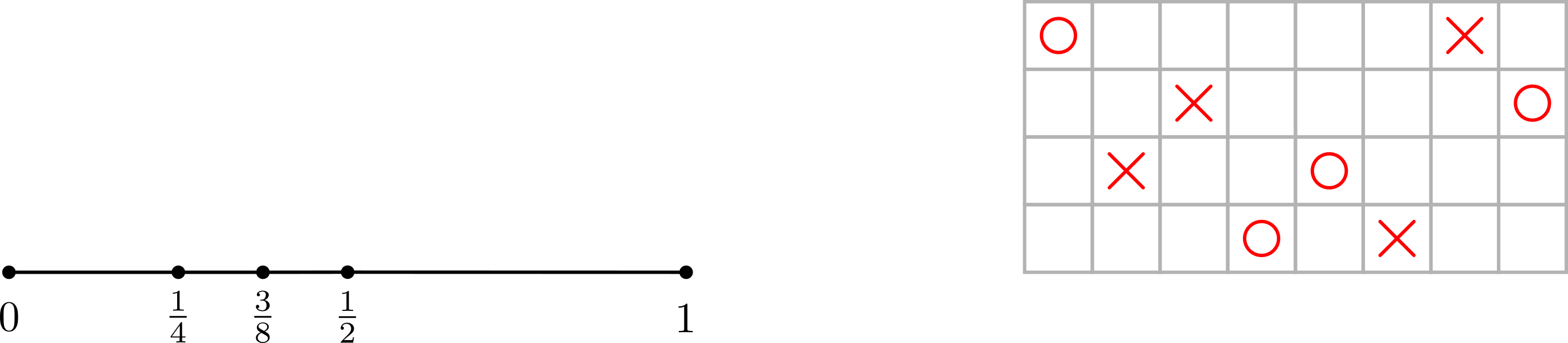
A half grid diagram is an grid of squares, each of which is either empty or contains an or an . We require that in each row there are exactly two nonempty squares, one containing an and the other containing an , and each column has exactly one nonempty square (which may contain either an or an ).
Definition 1.5.
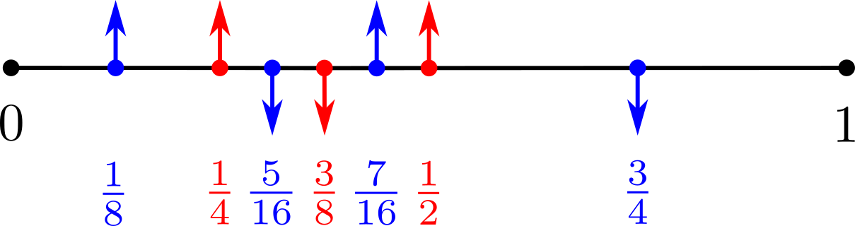
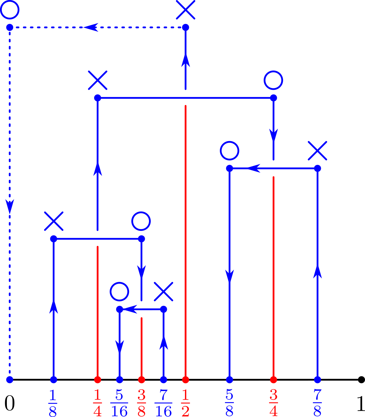
Let be an half grid diagram. The -oriented tangle associated to is defined by first connecting to in each row, then connecting each or to the bottom of the grid by vertical arcs, oriented upward in the case of an and downward in the case of an . We again use the crossing convention that horizontal segments are always above vertical segments.
See Figure 1(b) for an example of a half grid diagram and its associated tangle.
Remark 1.6.
Throughout the paper, we will view a grid or a half grid diagram as a subset of lattice points where the grid at the lower left corner corresponds to point . To describe a grid diagram or half grid diagram we just need to specify the coordinates of ’s and ’s on lattice points.
Next, we give a compatible condition describing when two half grid diagrams can reproduce a grid diagram.
Definition 1.7.
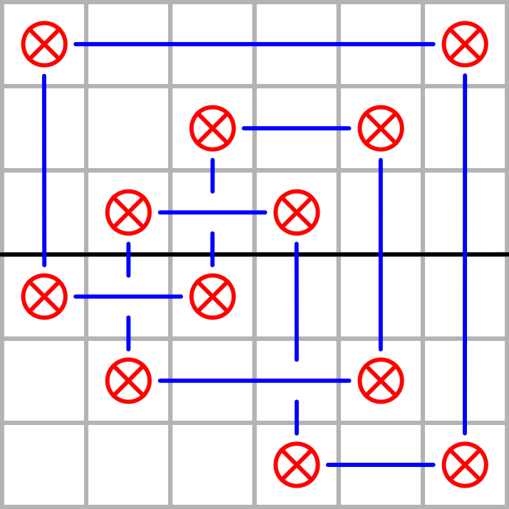
Let and be a pair of half grid diagrams. We say they are compatible, or say is a compatible half grid pair, if the column of and the column of contain the same symbol for each .
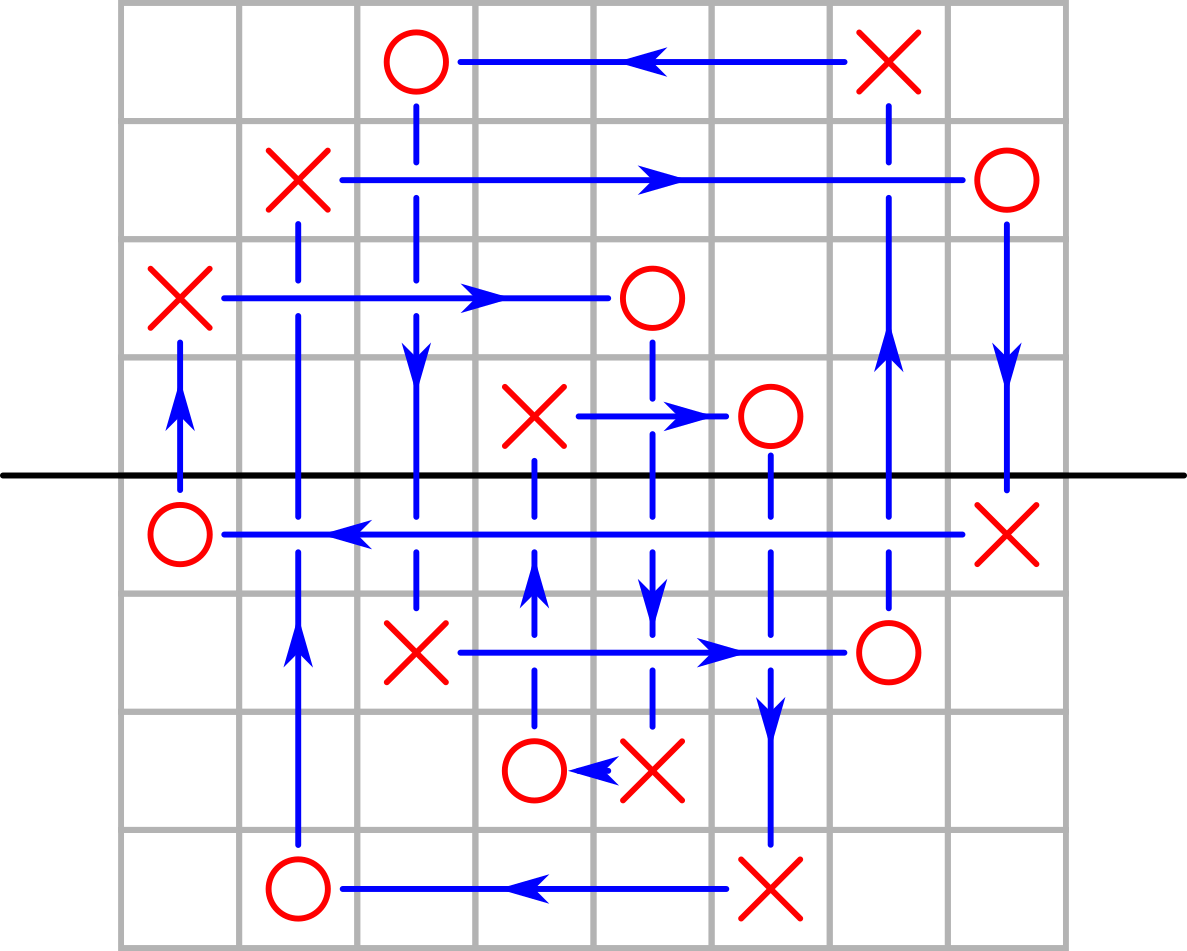
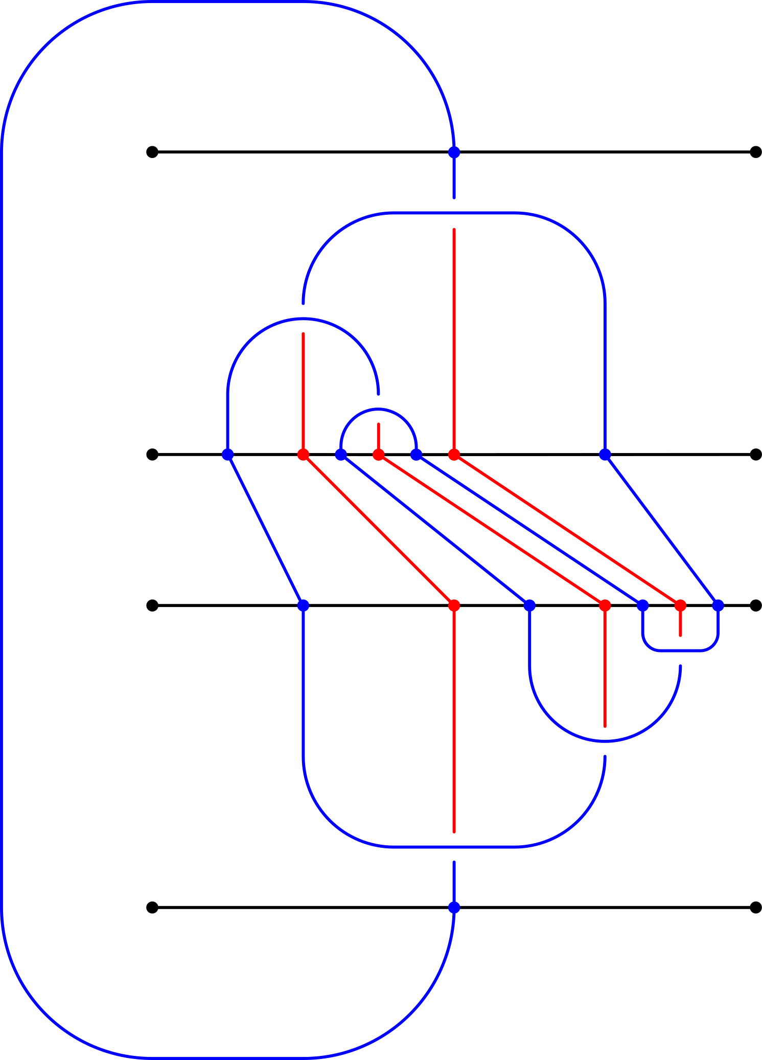
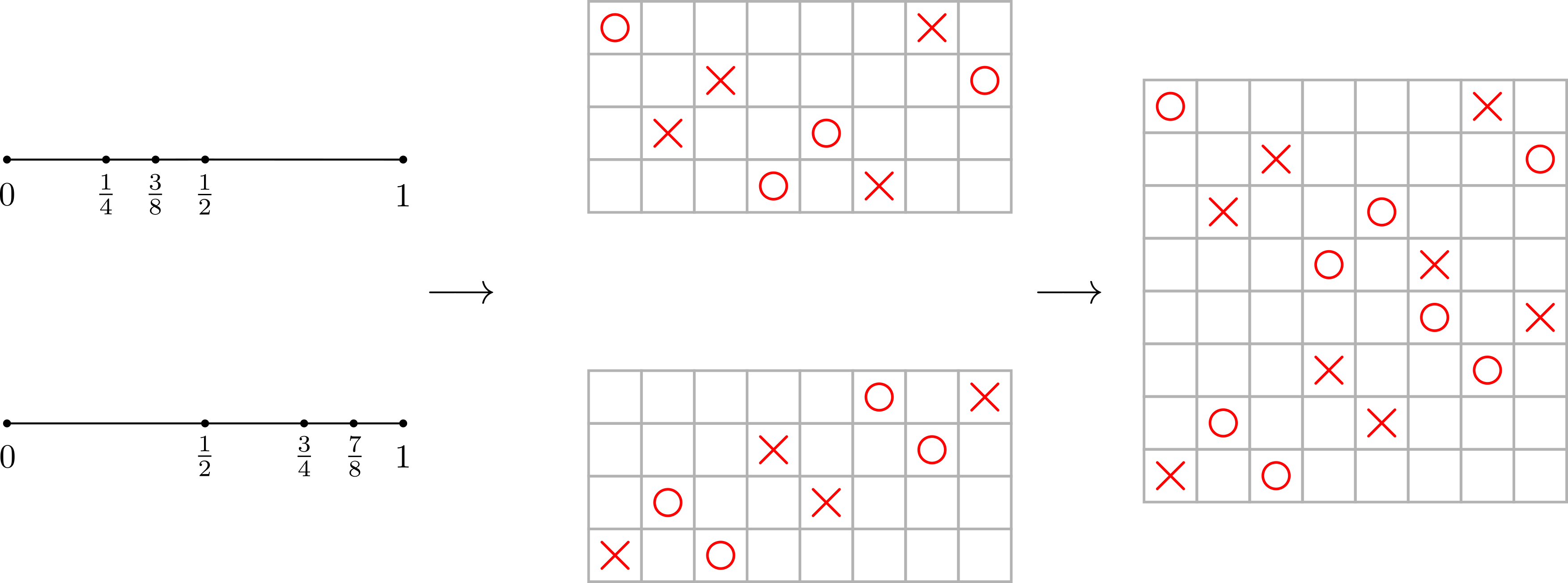
Given two compatible half grid diagrams and , we can obtain a grid diagram as follows: We first flip upside down and change each to and to to get , then we stack over (see Figure 2 for an example). The resulting diagram, still denoted as , is a grid diagram, because the the column of and the column of contain opposite markings for each . It is easy to observe that , where is the vertical mirror of with reversed orientation.
Remark 1.8.
Notice that and are not the same grid diagram, so the order of and matters. The relation between and is .
We just saw that any compatible half grid pair generates an oriented link . One can ask about the converse: can every oriented link be generated by a compatible half grid pair? We give an affirmative answer to it.
Definition 1.9.
An oriented link is half grid presentable if there exists compatible half grid diagrams and such that , and we call a half grid representative of .
Theorem 1.10.
Every oriented link is half grid presentable.
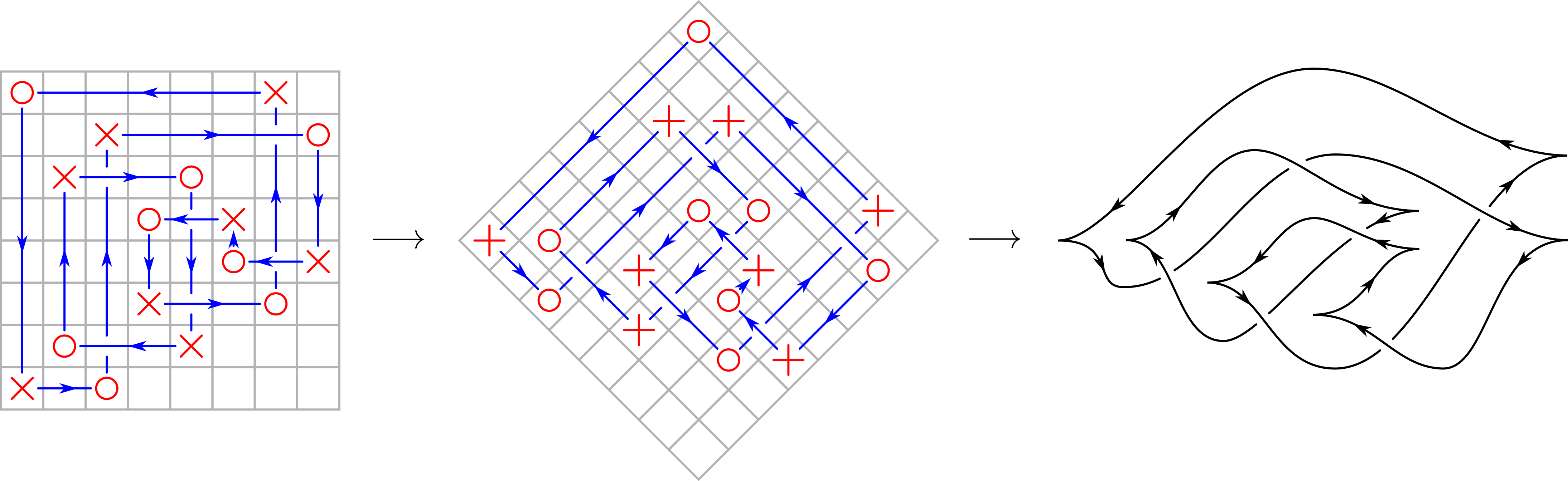
We will prove Theorem 1.10 by referring to the result in [1] that every oriented link is isomorphic to (called an oriented Thompson link) corresponding to some in the oriented Thompson group , then showing that every oriented Thompson link is half grid presentable (Section 4.2).
Half grid construction of links expands the bridge between classical link theory and Thompson link theory established by Jones. For example, our first application relates the number of link components to leaf number of Thompson group element. We denote the number of link components of oriented link as .
Theorem 1.11.
If has leaf number , then we have
Grid diagrams are closely related to front projection of the Legendrian links in with the standard tight contact structure. See section 5.1. In the second application, we provide a lower bound for both the maximum Thurston-Bennequin number and the maximum self-linking number of oriented knots in using the oriented Thompson index .
Theorem 1.12.
For any oriented knot in , we have
| (1.1) |
More generally,
| (1.2) |
where has reversed orientation of , and is the mirror of . Similarly, we have
and
Apart from the relation between contact geometry invariants and the oriented Thompson index, we also have purely topological relationships between some knot invariants and the (oriented) Thompson index.
Theorem 1.13.
For any oriented link , we have
where is the maximal Euler characteristic number along all Seifert surfaces of . As in the special case when is a knot, we have
where is the Seifert genus of .
Using the Thurston-Bennequin inequality and Theorem 1.12, we immediate have the following corollary which gives both upper and lower bound for and .
Corollary 1.14.
For any oriented knot , we have
and
After we see the unoriented version of half grid construction in Section 5.2.1, we can give an upper bound of the minimal grid number using unoriented Thompson index , as our third application.
Theorem 1.15.
For any link , we have
As a consequence of the relation between grid number , braid index , and bridge number , we have
Apart from its natural connection to Thompson links, the half grid presentation itself gives a “symmetric” way to describe links. The first set is to encode any half grid diagram by an element in symmetric group .
Theorem 1.16.
There is a one-to-one correspondence between half grid diagrams and elements in .
The correspondence is very simple, we just record where the and are in each row from bottom to top. For example, the half grid diagram in Figure 1(b) corresponds to
For a more detailed description , see Section 5.2.1.
Theorem 1.10 tells us that every oriented link can be generated by a pair of half grid diagrams. It turns out that we have a parallel result for link groups, stating that every link group has a “half grid presentation” encoded by a pair of symmetric group elements and .
Theorem 1.17.
A group is a link group ( for some link in ) if and only if for some positive integer and two elements , in , has the following presentation, called a half grid presentation.
| (1.3) |
where , with . In other words, we take away one by one from .
Acknowledgement
The authors would like to thank Slava Krushkal and Tom Mark for useful suggestions. Yangxiao Luo was supported in part by NSF grant DMS-2105467 to Slava Krushkal. Shunyu Wan was supported in part by grants from the NSF (RTG grant DMS-1839968) and the Simons Foundation (grants 523795 and 961391 to Thomas Mark).
2 Thompson group and standard dyadic partition
2.1 Background of Thompson group
We first give a brief introduction to Thompson group and related concepts.
Definition 2.1.
A standard dyadic interval (s.d. interval) is an interval of the form for some non-negative integer and some non-negative integer . A standard dyadic -partition (s.d. -partition) on is a partition such that is an s.d. interval for any .
We call a breakpoint of the s.d. partition, and call a subinterval of the s.d. partition. Suppose and are s.d. partitions, we denote if is a refinement of as partitions. In other words, the breakpoints of is a subset of the breakpoints of .
We denote the collection of all s.d. intervals as , and denote to be the trivial partition .
Definition 2.2.
Thompson group is the group (under composition) of homeomorphism ’s from to itself satisfying the following conditions:
-
1.
is piecewise linear and orientation-preserving.
-
2.
In the pieces where linear, the slope is always a power of .
-
3.
The breakpoints are dyadic rational numbers, i.e. for some and .
Definition 2.3.
Suppose that is a s.d. -partition with breakpoints , and is a s.d. -partition with breakpoints . We define to be the piecewise linear function determined by letting for all and letting be linear on for all .
Note that is an element in . We say is a pair of s.d. partitions representing .
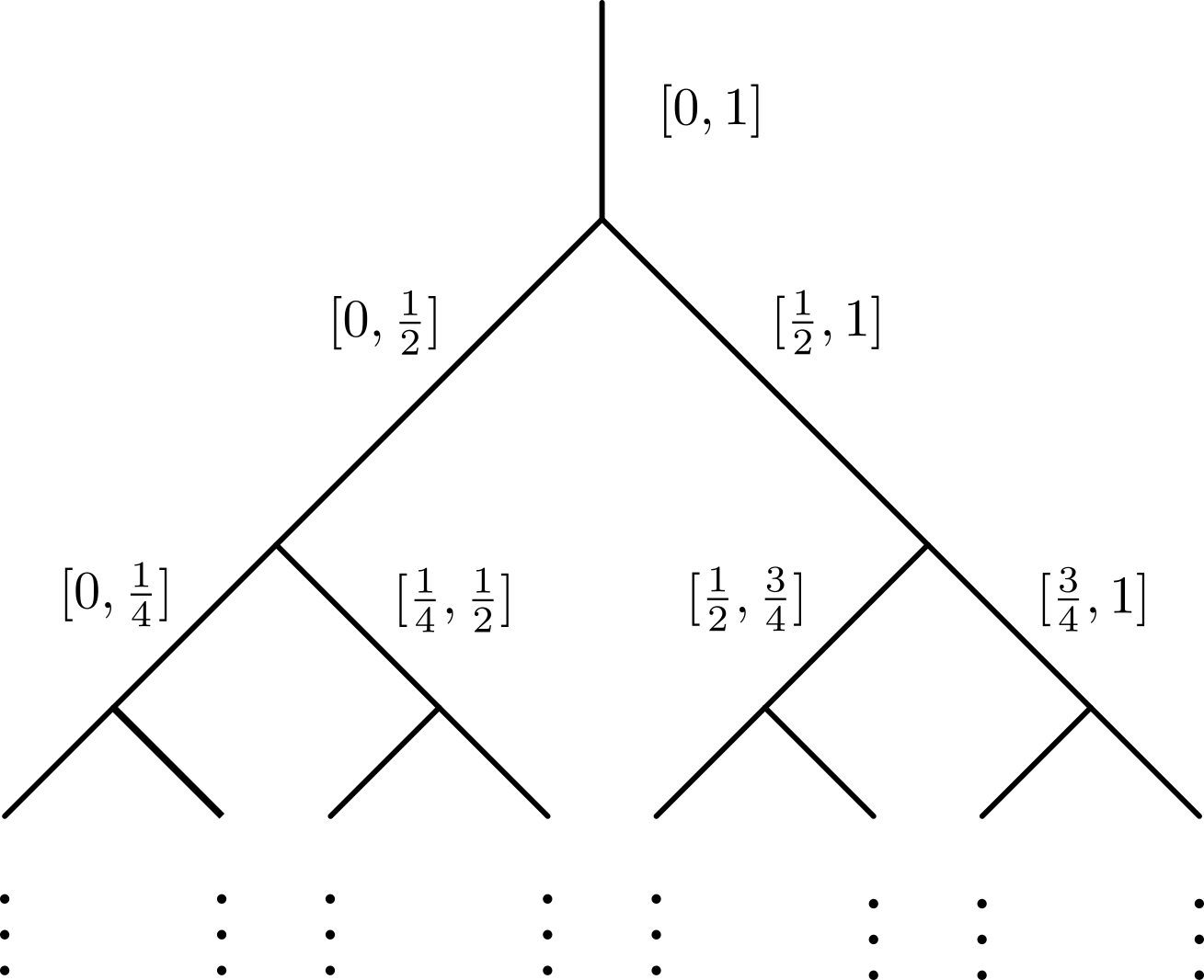
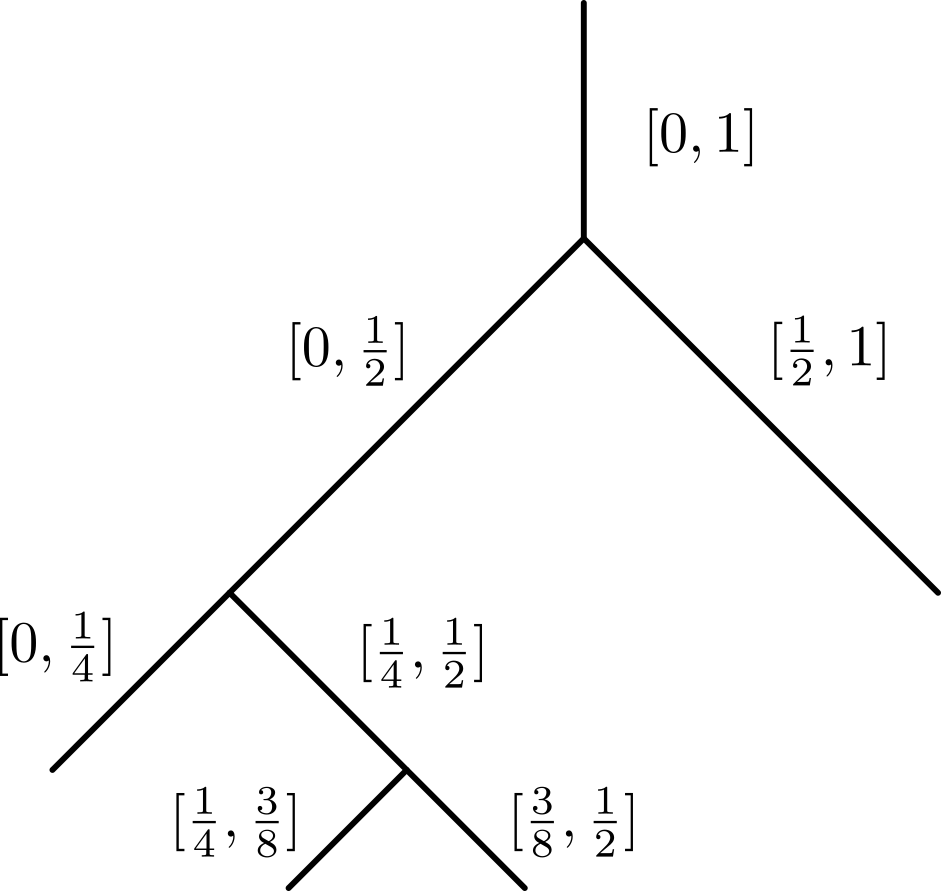
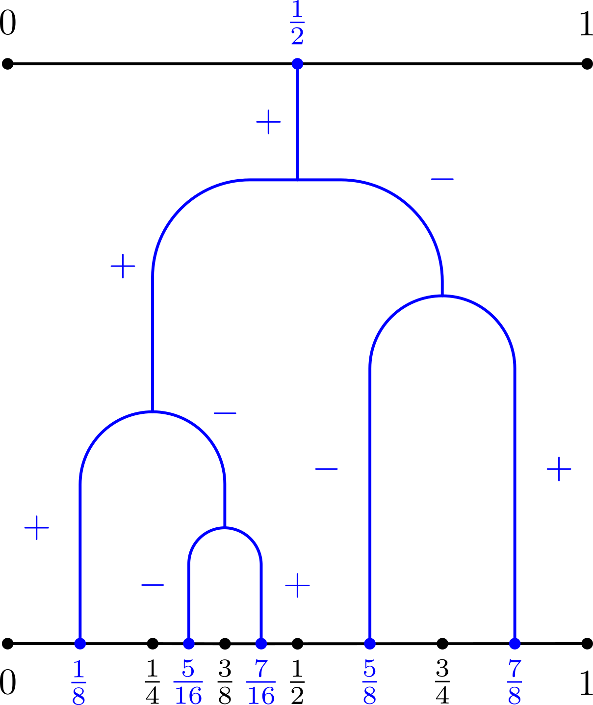
There is a bijection between the set of s.d. partitions and the set of binary trees. To illustrate that, first we label edges of the infinite binary tree (with an extra edge attached to the root) by standard dyadic intervals, such that the uppermost edge is labeled by and each trivalent vertex represents a cutting at the midpoint (see Figure 3). Note that this labeling gives a bijection , where is the collection of edges of .
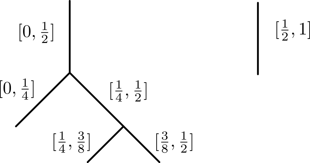
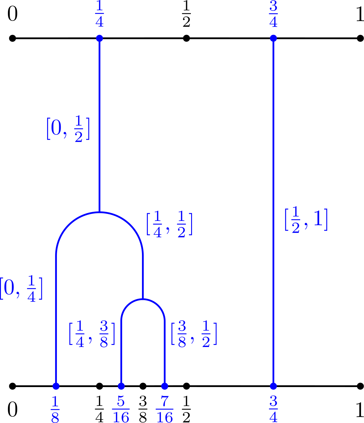
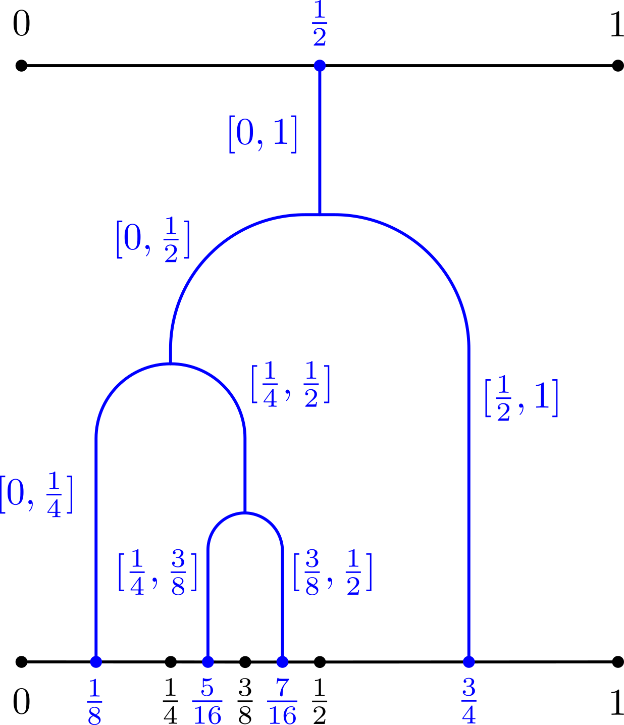
Given an s.d. partition , we can find a unique binary tree as a labeled subtree of whose uppermost edges are labeled by , and lowermost edges are labeled by subintervals of (see Figure 4(a) for an example). More generally, given a pair of s.d. partitions , we can find a unique forest as a labeled subgraph of whose uppermost edges are labeled by subintervals of , and lowermost edges are labeled by subintervals of (see Figure 4(b) for an example).
Using the notion of binary trees, we can visualize any pair of s.d. -partitions as a pair of binary trees with leaves. We often take the vertical mirror of and put it below , and call the resulting diagram a tree diagram of , also denoted as . Figure 5(a) is an example of a tree diagram.
Given two pairs of s.d. partitions and , we say that is a refinement of if can be obtained by adding some “carets” to , as Figure 5(b) shows. Equivalently, are refinements of respectively, and these two refinements are linearly compatible, i.e. .
We say a pair of s.d. partitions is reduced if it is not a refinement of any other pairs. In other words, contains no carets.
Lemma 2.4.
[3, Lemma 2.2] Any has a unique reduced pair of s.d. partitions representing it. Furthermore, any pair representing is a refinement of .
If is a pair of s.d. partitions representing , we say is a tree diagram of . If is the reduced pair of s.d. partitions representing , we say is the reduced tree diagram of . In the latter case, the leaf number of or is called the leaf number of .
2.2 Some general theories of standard dyadic partition
In later sections, we will construct half grid diagrams based on s.d. partitions. First we need to introduce some useful notations and properties related to s.d. partitions.
Definition 2.5.
A left (resp. right) s.d. interval is an s.d. interval of the form for some even (resp. odd) number and some integer . We denote the collection of left (resp. right) s.d. intervals as (resp. ).
According to the above definition, is neither a left s.d. interval nor a right s.d. interval. However, we will regard as a right s.d. interval. With this convention, any s.d. interval is either a left s.d. interval or a right s.d. interval, but cannot be both simultaneously. As a consequence, is the disjoint union of and .
Definition 2.6.
Let , we define the conjugate of to be
is called the conjugate of .
In the previous section we described a bijection . We can easily see that for any , is a left (resp. right) interval if and only if is a left (resp. right) edge. Furthermore, splits into and at a trivalent vertex.
Next definition will play the key role in the construction of half grid diagrams.
Definition 2.7.
Let be an s.d. partition with breakpoints . We denote to be the collection of ’s such that is a s.d. interval. Denote and .
Recall that can be represented by a binary tree as a subtree of . If we restrict the bijection on , we have a bijection , where is the collection of edges of . This bijection sends subintervals of to the lowermost edges of , and other s.d. intervals to non-lowermost edges.
Observe that each non-uppermost edge must be a split of , and each non-lowermost edge can split into and for some , then we have the following lemma.
Lemma 2.8.
Suppose , then . Furthermore, if is not a subinterval of , then for some .
By counting the number of edges of , we get the following lemma.
Lemma 2.9.
Let be an s.d. -partition, then
-
1.
-
2.
Next, we turn to dyadic rational numbers and their connection to s.d. intervals and the Thompson group.
Definition 2.10.
We denote , the set of dyadic rational numbers except and . Given an s.d. partition , denote to be the set of midpoints of subintervals of . Denote to be the union of and all of breakpoints of except and .
Note that and are both subsets of .
Lemma 2.11.
The map , sending s.d. intervals to their midpoints, is a bijection. Furthermore, is a bijection for any s.d. partition .
Proof.
Note that has inverse sending any dyadic number with some not divided by 2, to an s.d. interval . So is a bijection.
To show is a bijection, we just need to show sends onto , then the statement follows since if is an -partition. Indeed, for any , if is a subinterval of , then . If is not a subinterval of , then for some by the last part of Lemma 2.8, so is a breakpoint of . ∎
In the next lemma, we will consider elements in the Thompson group as homeomorphisms from to itself.
Lemma 2.12.
For any , we have that is a bijection. Furthermore, if is represented by a pair of s.d. partitions , then is a bijection.
Proof.
First of all, we have . To show it, we take the reduced s.d. partition pair representing . For any , we can always choose refinement such that is a breakpoint of . Notice that also represents , so sends to a breakpoint of , which is in .
Notice that is the inverse of , so is a bijection.
To show is a bijection, we just need to show sends into , then the statement follows since . Indeed, by Definition 2.3, we know that sends breakpoints of to breakpoints of , sends to due to linearality of on each subinterval. ∎
3 Thompson link
3.1 Jones’ construction of links from Thompson group
Let be the planar algebra of Conway tangles, where has basis Conway tangles with boundary points. For Conway tangles, we identify two tangles if they differ by a family of distant unlinked unknots. For example, is spanned by links up to distant unlinked unknots, is spanned by tangles with two boundary points, up to distant unlinked unknots. We denote the class of trivial tangle in as .
Moreover, has a -valued inner product structure , given by connecting boundary points of to boundary points of one by one (see Figure 6).
Definition 3.1.
Let be the category of tangles, with objects s.d. partitions, and morphisms for being tangles with marked boundary points on the top and on the bottom. For a tangle , we denote to be the vertical mirror of .
Suppose that we have a pair of s.d. partitions in . Recall that we have a forest such that each lowermost edge is labeled by subintervals of and each uppermost edge is labeled by subintervals of . Now we embed into such that each lowermost edge has lower endpoint , each uppermost edge has upper endpoint . By this embedding, we can regard as a forest whose roots are and whose leaves are .
For each edge of , we denote the vertical projection of ’s lower vertex as . Now we further isotope in such that for any edge , then we can regard as a map from to . Specifically, is a bijection, because and both of , are bijections. See Figure 7(a) and 7(b) for examples of an embedded forest and an embedded tree.
Definition 3.2.
Given a pair of objects in , a labeled tangle is defined by replacing each trivalent vertex of the forest by an instance of , with a vertical straight line joining the bottom of the disc containing to the breakpoint of below the replaced vertex, and vertical lines connecting all the breakpoints of to those breakpoints of in common with .
In the rest of this section, we choose to be the crossing with a horizontal strand crossing over a vertical strand, as shown in Figure 8.
In the construction of tangle , every edge of becomes an arc of , called a Type A arc. If is not an lowermost edge, then we need to add a vertical arc extending to breakpoint . Such an arc is called a Type B arc. At last, we need to add some arcs to connect breakpoints, and these arcs are also called Type B arcs.
In [6] Jones considered a representation of the category , associating each s.d. interval with subintervals a vector space . Then take the direct limit over the ordered set , with linear map from to induced by the canonical morphism . The resulting space has an inner product induced by the inner product on .
Definition 3.3.
Suppose that is represented by a pair of s.d. partitions , not necessarily reduced. Then define to be the tangle with straight lines connecting points of to points one by one.
Remark 3.4.
In Lemma 2.12, we showed that is a bijection. Here visualizes this bijection. connects any to .
Jones also defined a representation of on . Suppose that corresponds to a reduced pair of s.d. partitions , given a vector , we first find a representative such that . Correspondingly, has an expression for some . Then the action of on is defined to be induced by the trivial tangle .
As a result, a link class (up to distant unlinked unknots) arises as a coefficient of .
Proposition 3.5.
[6, Theorem 5.3.1] For any , there exists such that .
Next, we will see an explicit construction of a link in the class . Notice that any representative of in can be written as for some , so it is not surprising that we can rephrase the above construction using only trees. For convenience, we will denote as , as and as .
Given , suppose that is a pair of s.d. partitions representing . Then we have a pair of binary trees and . Furthermore, we have , as shown in Figure 10(a). Then we close it up to get a link in the class , where is a representative of , and is a representative of .
We let be , where is unique reduced pair of s.d. partitions representing . Notice that for a non-reduced pair representing , contains some distant unknots compared to as shown in Figure 10(b), but and are in the same link class in .
At last, if we consider and as -tangles with unmarked endpoints, and as a trivial -tangle with unmarked endpoints, then is simply the closing-up of . Equivalently, we add a trivial strand on the leftmost of and respectively, then cap them off on the top to get -tangles and . Then , as shown in Figures 11(a) and 11(b). Notice that this notion is irrelevant to the Thompson group, is completely determined by a pair of s.d. partitions with the same number of breakpoints.
In fact, what Jones proved in [6] is slightly stronger than Proposition 3.5, as the following theorem states.
Theorem 3.6.
Given any unoriented link , there exists such that .
This theorem is the analog of the “Alexander theorem” for braids and links. It establishes that the Thompson group is in fact as good as the braid groups at producing unoriented links. So we can define Thompson index of unoriented links as an analogue of the braid index.
Definition 3.7.
Given an unoriented link , we define its Thompson index to be the smallest leaf number required for an element of to give rise to .
3.2 Oriented Thompson group and oriented Thompson link
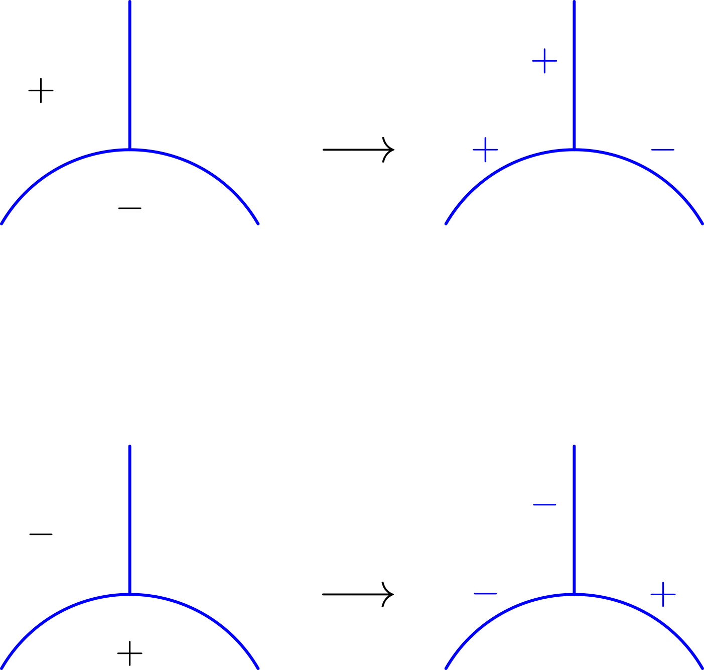
In the previous section we saw how to construct from for s.d. -partition . Now we show how to give the canonical orientation to from the signed region of ’s complement, following [2]. Given binary tree embedded in , the complement of has regions. We assign to the leftmost region, then apply the rules shown in Figure 12(a) times to assign signs to all other regions except the rightmost one. See Figure 12(b) for an example.
Definition 3.8.
For , an -sign is a sequence of ’s and ’s such that the first sign is and the second is (if ).
Suppose is an s.d. -partition with breakpoints , then induces an -sign such that the sign in is the sign of the region above breakpoint .
Definition 3.9.
The oriented Thompson group is the collection of ’s in such that for some s.d. -partition pair representing , their corresponding signed trees and induce same -sign .
Remark 3.10.
In Definition 3.9, we can replace “some s.d. -partition pair” by “any s.d. -partition pair”. Indeed, suppose that the tree diagram is obtained from by adding a caret at the leaf. From the rules shown in Figure 12(a), to obtain from , we just need to replace the sign of by if the original sign is , by if the original sign is . So if and only if .
Remark 3.11.
The notation of -sign was introduced in [2], where is described as group of fractions of a category . It turns out that Definition 3.9 is equivalent to the definition of as group of fractions. See Appendix A for more details.
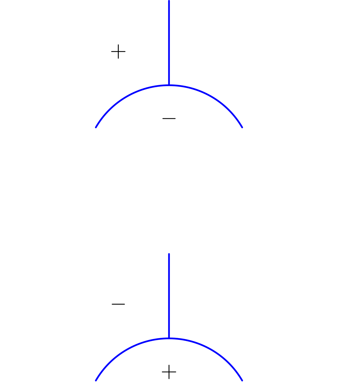
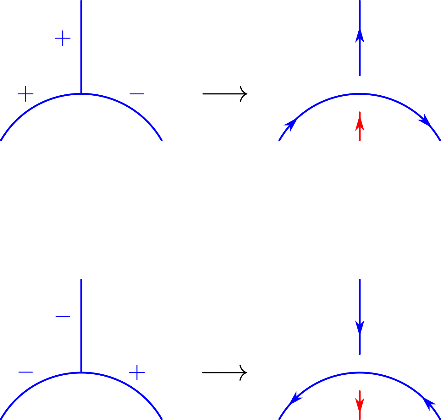
Suppose that is a tree with signed regions. When we add vertical strands to construct , each strand separates each signed region into two regions, we move the sign to the right region of the added strand. To obtain the canonical orientation on , we let each -signed region induce counterclockwise orientation on its boundary arcs, and each -signed region induce clockwise orientation on its boundary arcs. See Figure 13(a) for an example.
Equivalently, the above procedure can be expressed locally as shown in Figure 13(b). It shows that the induced orientations of arcs are compatible around each crossing. We denote the oriented as .
Furthermore, induces a canonical signing on as the lower boundary of . We let upward orientation induce sign , let downward orientation induce sign . For instance, contains a single point with the sign. See Figure 13(c) for another example. Notice that the signing on is determined by the -sign induced by . More specifically, the sign on the midpoint is the ame as the sign, and the sign on breakpoint is opposite of the sign on midpoint . Conversely, can be recovered by taking signs on midpoints in .
Recall if a pair of s.d. partitions represents an element , then is the close-up of . However, if we replace by and replace by , we need to have some orientation compatible with the orientations of and . In other words, we need and to have compatible signings.
Definition 3.12.
Let and be a pair of s.d. partitions with the same number of breakpoints, we say and are compatible, or is a compatible s.d. partition pair if represents an element .
By Remark 3.10, if is a compatible pair representing , then and induce same -sign, which determines compatible signings on and . Then can be assigned a unique compatible orientation, denoted as . We let be the oriented link obtained by closing up the oriented tangle . Similar to the unoriented scenario, we have a description in terms of -tangles. We can first add a trivial strand on the leftmost of and respectively, with orientation from bottom to top. Then cap them off to get -tangles and . We have .
Lemma 3.13.
Let be an s.d. -partition, then the oriented -tangle has crossings and all of them are positive. Furthermore, if is a compatible s.d. partition pair, then has writhe .
Proof.
Each crossing in comes from one of trivalent vertices of , and it must be one of the two cases shown in Figure 15(b). Notice that either case generates a positive crossing, so has positive crossings.
Now suppose is a compatible s.d. -partition pair, then has positive crossings, has negative crossings. So has writhe . ∎
Recall that when is the reduced pair of s.d. partitions representing , we denote as . So also has an orientation . Unless otherwise stated, we will consider every link and tangle as oriented and omit arrow notations in the rest of this paper, except Section 5.2.1.
There is also an Alexander theorem for the oriented Thompson group .
Theorem 3.14.
[1] Given any oriented link , there exists such that .
So similar to the unoriented Thompson index of unoriented links, we can define oriented Thompson index of oriented links.
Definition 3.15.
Given an oriented link , we define its oriented Thompson index to be the smallest leaf number required for an element of to give rise to .
4 Grid Construction for oriented Thompson link
In this section we will introduce half grid construction from s.d. partitions, and grid construction from elements in . In Section 4.1 we first introduce signs on s.d. intervals, and we give an algebraic definition of based on those signs. Section 4.2 is our main construction, using “midpoint order” and “length order” along with signs of s.d. intervals, to construct half grid diagram. Then we show the algebraic definition of implies compatibility of two half grid diagrams given by . In Section 4.3 we show this grid construction is equivalent to Jones’ construction of oriented Thompson link. In the end, we prove our main theorem that every oriented link is half grid presentable.
4.1 Signs of standard dyadic intervals and an algebraic definition of oriented Thompson group
Given an s.d. partition with breakpoints . Recall that is the collection of ’s such that is an s.d. interval. We want to construct a half grid diagram , such that each s.d. interval corresponds to a marking in .
To achieve this we need to determine what and where these markings are. We first introduce the sign function on , the set of all s.d. intervals.
Definition 4.1.
Define to be the map uniquely determined by the following conditions.
-
1.
-
2.
For any , we have
Note that the above conditions in fact give us an inductive definition of . Condition 1 tells us , then we know and by condition 2. Generally, we can apply the second condition times to get the value of on an s.d. interval of length .
Recall that is the set of rational dyadic numbers except and , and we have a bijection , sending s.d. intervals to their midpoints. Then we put signs on so that and have the same sign for any . Also recall Lemma 2.12, stating that any restricted on is a bijection from to itself.
Definition 4.2.
Define to be the subset of consisting of homeomorphisms that preserve signs on .
Note that if preserve signs on , then also preserves signs on . Thus, is a subgroup of .
Theorem 4.3.
as subgroups of .
Before we prove Theorem 4.3, we first give an equivalent definition of the canonical orientation of . Recall that given an s.d. -partition , the embedded tree separates into regions, and each region has a sign except the rightmost one. Now we assign signs to all of the edges of instead, by letting each edge have the same sign as the region on its left. Correspondingly, rules of assigning signs on regions become rules of assigning signs on edges as Figure 15(a) shows, and the requirement that the leftmost region has sign becomes the requirement that the uppermost edge has sign .
In Section 2.2 we saw a bijection sending left intervals to left edges, right intervals to right edges. The signs on are given by the sign function , defined by the recursive rules in Definition 4.1. Note that those rules are the same as the recursive signing rules (Figure 15(a)) on up to the bijection . Then we get the following lemma.
Lemma 4.4.
is a sign-preserving bijection.
Notice that we can get the canonical orientation of using signs on the edges of instead, because we just moved signs from regions to edges. So similar to the local rules to assign orientation of in terms of signed regions (see Figure 13(b)), we have corresponding local rules based on signed edges, shown in Figure 15(b). See Figure 15(c) for an example of recovering the canonical orientation of from the signed edges of .

Recall that each point in has a sign induced by the canonical orientation of .
Lemma 4.5.
is a sign-preserving bijection.
Proof.
Suppose that , then is either a breakpoint of or a midpoint of a subinterval of . If is a breakpoint, then it is attached to a Type B arc of , which extends Type A arc to . From Figure 15(b) and 15(c), we can observe that a Type A arc has an upward orientation if has sign , downward orientation if has sign . Since the sign of is induced by , which extends the orientation of , we must have the same sign on and . If is a midpoint, then it is attached to Type A arc directly, so and have the same sign. ∎
Thus, we have a sign preserving bijection , where the signs on are given by the sign function , the signs on are induced by the canonical orientation of . In other words, the signs on can be equivalently obtained from the signs on , by taking midpoints. Notice that it is exactly how we defined signs on .
Proof of Theorem 4.3.
Suppose that . For any , we can find an s.d. partition pair representing such that is a breakpoint of . Remember that the signs on and are determined by and , respectively. So implies that the sign of and the sign of are same for any . By Lemma 2.12 and the fact that is increasing, we know that sends the point of to the point of for any . Thus and have the same sign. It is true for any , so .
Conversely, suppose that preserves signs on . Take an s.d. partition pair representing , then for any , and have the same sign. In other words, the sign of and the sign of are same for any . Recall that and can be obtained by taking signs of midpoints in and respectively, so we have . Thus . ∎
Before we move on to the next section, let’s first introduce some notations related to signs on . We denote and . An element in is called a positive s.d. interval, an element in is called a negative s.d. interval. From the definition of , we can easily observe that taking conjugate of will change its sign.
Combine this observation with Lemma 2.9, and notice that has no conjugate, we have the following lemma.
Lemma 4.6.
Suppose that is an s.d. -partition, then
-
1.
-
2.
4.2 Half grid construction
Given an s.d. -partition , now we are ready to define position functions and on , through the following two orders on .
Definition 4.7.
Let represent the set with two partial orders and . For , we define if . Define if either the length of is strictly less than the length of , or the length of equals the length and .
It is easy to check that both of and are total orders on .
We first restrict the midpoint order on . Since is a total order, elements in can be ordered as . We define a bijection
Then restrict the length order on and reorder elements in as . Notice that is always . We define
Then and are both bijections.
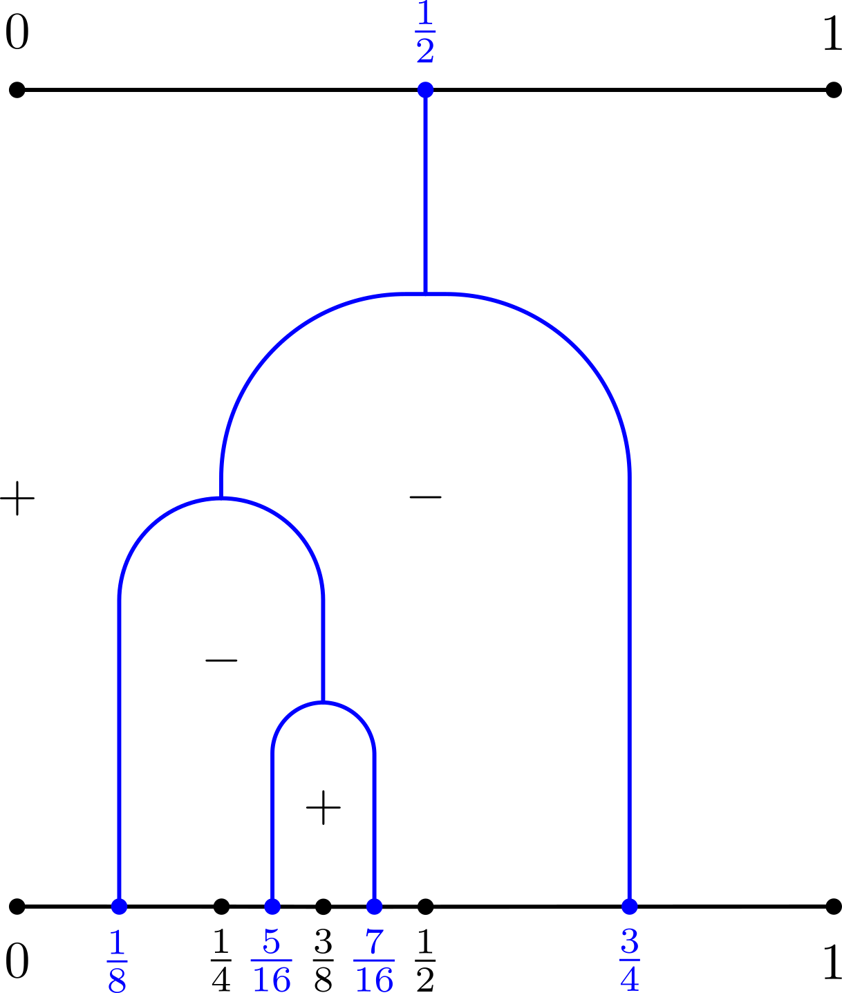
Next, we will show how to construct an half grid diagram associated to . First, we always assign marking to the entry by default. Then we let each s.d. interval assign a marking to the entry in the grid, where the marking is if , if . We denote the resulting diagram as .
Proposition 4.8.
is a half grid diagram.
Proof.
First, it is impossible that there exists any entry with two markings, because is a bijection.
Then we need to show that each column has exactly one marking and each row has an and an . Indeed, the at the entry is the only marking in the first column. For any , let , then the or at the entry is the only marking in the column, because is a bijection. For any , let , then the at the entry is the only in the row, because is a bijection. If , then . By the definition of , we have . Then the at the entry is the only in the row, because is a bijection. At last, the at the entry is the only in the row. ∎
Now suppose that we have a pair of s.d. partitions with same number of breakpoints, we want to know whether and are compatible, so that we can put them together to obtain a complete grid diagram . It turns out that the answer is affirmative if represents an element . Recall that such a pair is called a compatible pair in Definition 3.12.
Proposition 4.9.
If is a compatible s.d. partition pair, then is a compatible half grid pair.
Proof.
We reorder s.d. intervals in and as
Reorder points in and as
By Lemma 2.11, we have a bijection sending an s.d. interval to its midpoint. Furthermore, preserves the midpoint order on . So must be the midpoint of , and must be the midpoint of .
Now suppose is a compatible s.d. partition pair representing . By Lemma 2.12 and the fact that is increasing, is a bijection sending to (for an illustration, see Figure 9). By Theorem 4.3, we know that and have the same sign for any .
Recall that we assigned signs on through the bijection , so and also have the same sign for any . By the construction of a half grid diagram, the column of contains a single marking if , if . It’s similar for the column of . Also notice that the first column of and the first column both contain an , so and are compatible. ∎
Theorem 4.10.
Suppose that is a compatible s.d. partition pair, then
as oriented links. Especially if is the reduced s.d. partition pair representing some , then .
We will prove the above theorem in the next section. Assuming Theorem 4.10, our main theorem follows immediately.
4.3 Equivalence to Jones’ construction
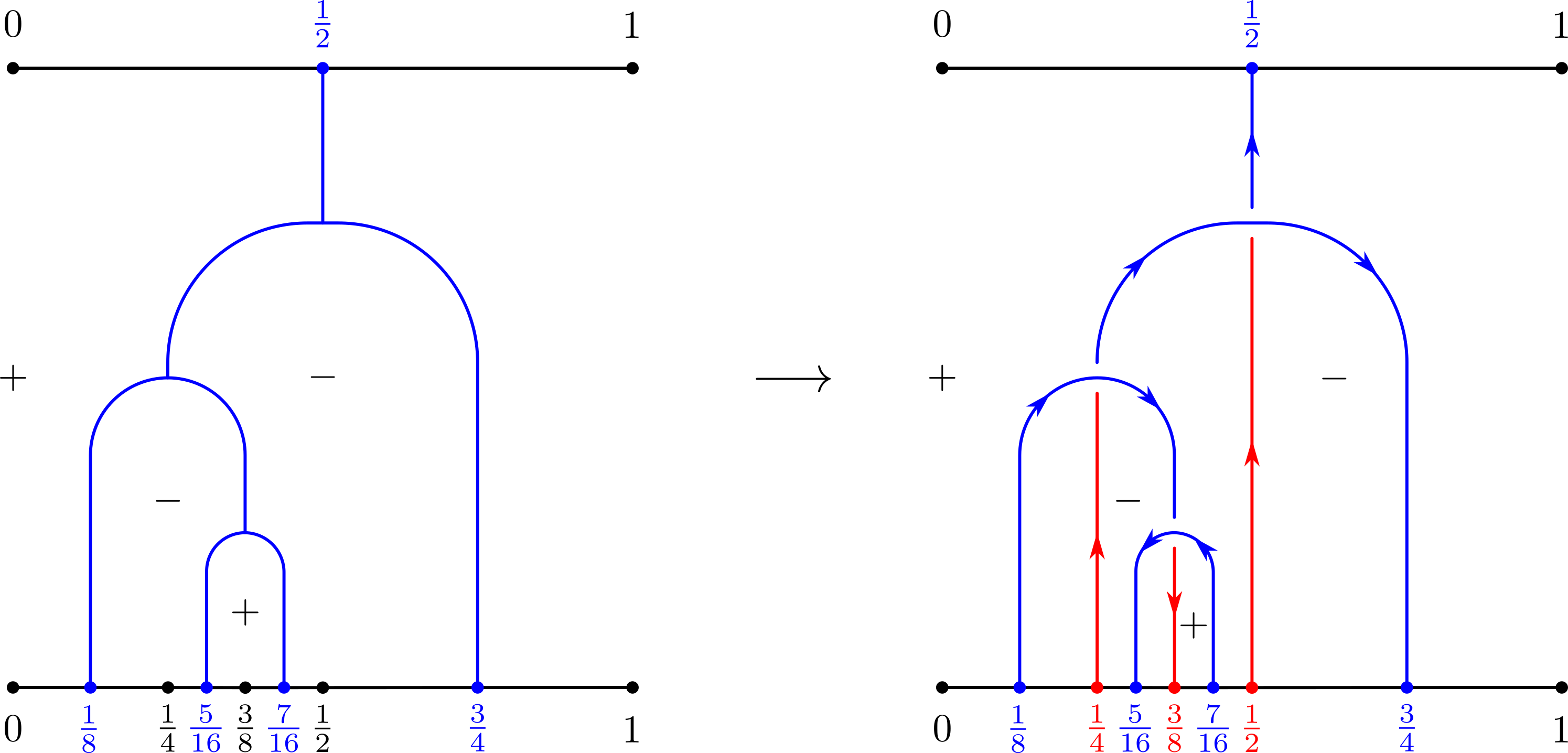
Given an s.d. -partition , in Section 3.2 we have an oriented -tangle coming from Jones’ construction, and in Section 4.2 we also have an oriented -tangle coming from half grid diagram construction. We claim that these two oriented tangles are actually same.
Proposition 4.11.
Let be an s.d. partition, then as oriented -tangles.
Proof.
First we move the trivalent vertices of vertically corresponding to their depth on the tree, so that vertex of smaller depth always has larger -coordinate. If two vertices are of same depth, we let the vertex on the right has larger -coordinate. See Figure 18(a) for an example of pre-isotoped tree .
Recall that when we turn a tree into a tangle , each edge of becomes a Type A arc of . If is not a lowermost edge, then we add vertical Type B arc extending to . See Figure 18(b) for an example, where Type A arcs are marked in blue and Type B arcs are marked in red. Now we keep Type B arcs unchanged and redraw Type A arcs as follows.
If is a left edge, we redraw as , and let be the upper-left corner. If is a right edge, we redraw as , and let be the upper-right corner. Then we consider the top edge attached to as a right edge and put an upper-right corner at . So the corresponding arc first goes upward to then turn left. We let it stop at and put an upper-left corner there to make it turn downwards until it hits .
After we redraw Type A arc , we label its corner by if has sign , by if has sign . For example, the corner at always has marking . As the last step, we mark the corner at by . See Figure 18(b) and Figure 18(c) for the described isotopy and markings.
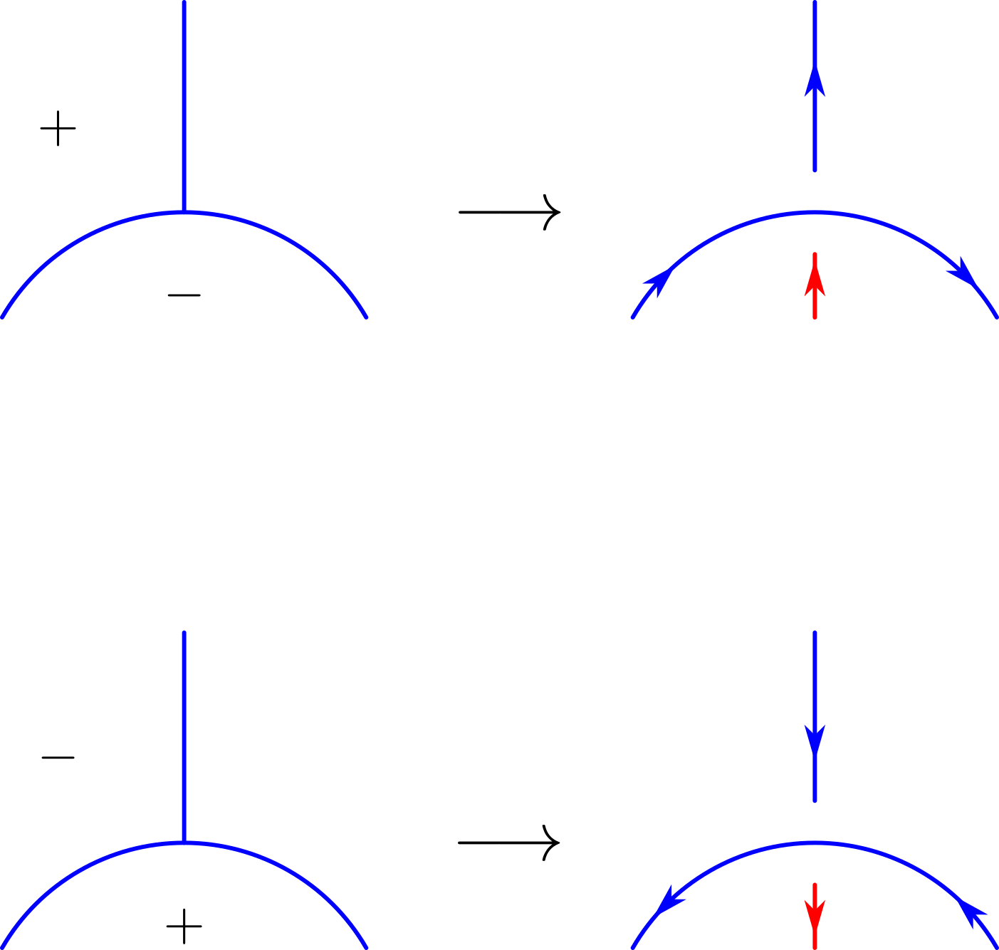
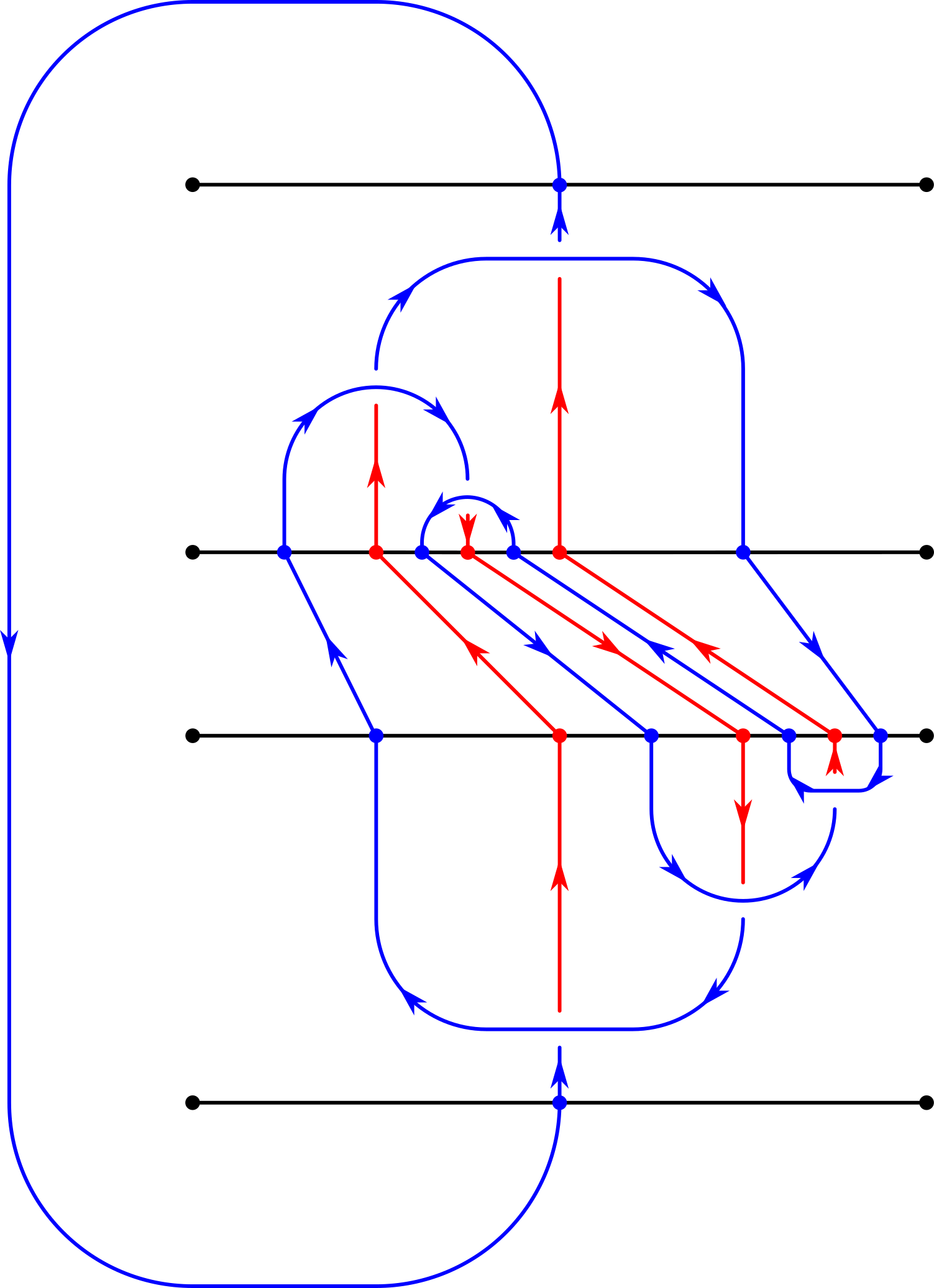
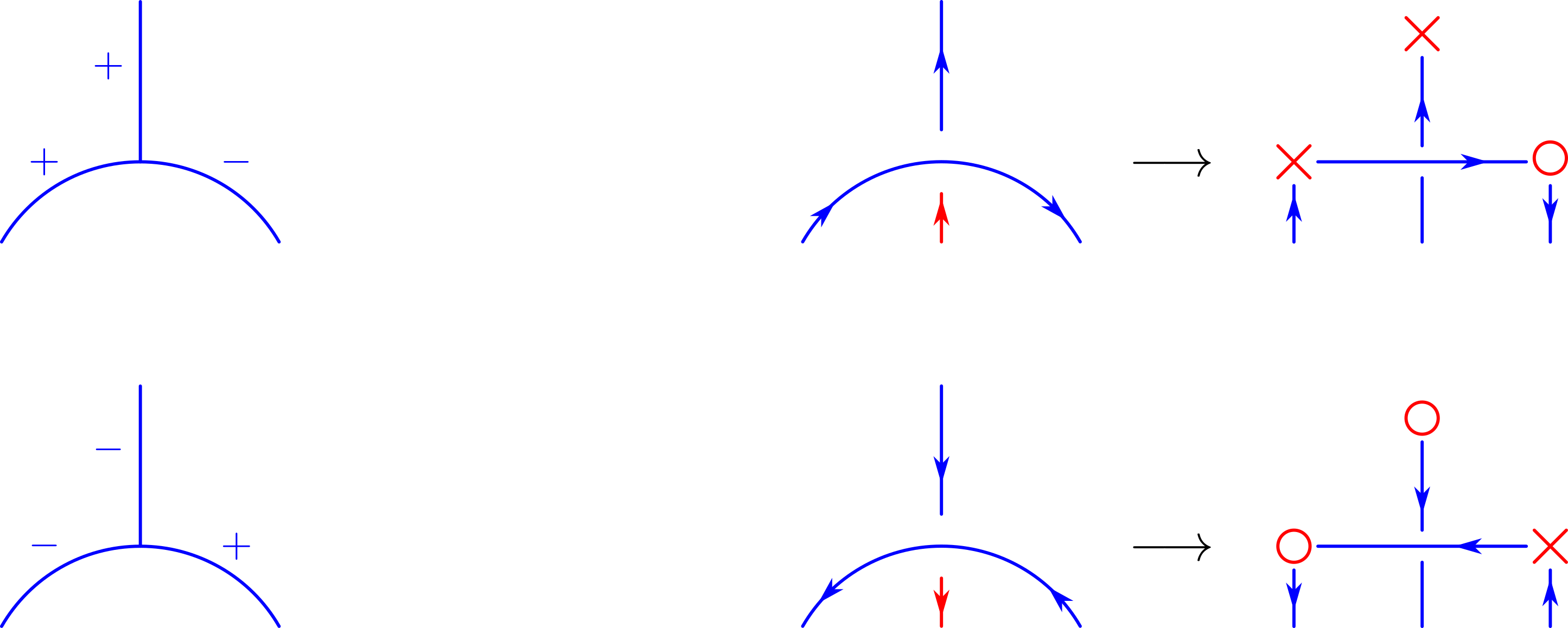
Now, note that the -coordinate of corner is the midpoint of , which is exactly . So for each point in , there is exactly one marking above it, and there is one marking at above . Also, for each trivalent vertex, there is exactly one marking on its left and one marking on its right, corresponding to its left edge and right edge, respectively. These two markings must be different, because the left edge and right edge of a same vertex have different signs (see Figure 15(b)). At last, there is an at and an at with -coordinate . Thus, if we rescale into vertically and horizontally to make sure that each marking has integer coordinates and regard as a half grid, then we get a half grid diagram . See Figure 18(c) and Figure 18(d) for an example.
The above transformation can also be expressed locally as Figure 19 shows, and capping off is equivalent to adding corners at and . So we have
Now, given any , notice that the coordinate of is the position of midpoint in the normal order (the first index is , because of the marking at the entry). It is same as the position of in the midpoint order, which is exactly . The coordinate of is the position of ’s upper endpoint in the reversed depth order. It is also the position of or in the length order, which is .
To show , it remains to show that they have the same marking in the entry. For , this marking is given by the sign of . For , this marking is given by the sign of . By Lemma 4.4, and have the same sign. So we have .
Thus, finally we have . ∎
Now we put two half grid diagrams together to prove Theorem 4.10.
5 Applications
5.1 Legendrian, transverse knot and half grid diagram
We first give a very brief introduction to the contact 3-manifold and Legendrian, transverse knot (see [5] for details).
Definition 5.1.
A contact 3 manifold is a smooth 3 manifold together with a 2-plane field distribution such that for any -form with , we have .
Definition 5.2.
A Legendrian link in is a disjoint union of embedded ’s that are always tangent to .
Definition 5.3.
A transverse link in is a disjoint union of oriented embedded ’s that are always positively transverse to .
We will only consider the oriented Legendrian knot in standard tight contact structure in given by . We can explicitly describe an oriented Legendrian link using the front projection .
Here are some basic properties of a front projection of a Legendrian link (see Figure 20).
-
1.
There is no vertical tangency in .
-
2.
The vertical tangencies change to generalized cusps, and the generalized cusps are the only non-smooth points.
-
3.
At each crossing the slope of the overcrossing is smaller than the undercrossing.
Moreover, using the front projection, we can combinatorially define two classical invariants of Legendrian link.
Definition 5.4.
Given a front projection of of a Legendrian link , the Thurston-Bennequin number of can be defined to be
and the rotation number of to be
The max Thurston-Bennequin number of a is the maximum value of among front projections of Legendrian knot having the same knot type as .
We also have a classical invariant associate to a transverse link called the self-linking number (we omit the definition for and refer readers to see [5] for details). For an oriented knot the max self-linking number of is the maximum value of self-linking numbers among all transverse representatives of . Moreover, We can always take the transverse push-off of a Legendrian link and their classical invariants are related by .
Now we are moving to the lemmas we need to prove Theorem 1.11.
Lemma 5.5.
Let be any front projection of a Legendrian link with components, we have
Proof.
Suppose , where is Legendrian knot component of . Let be the front projection of by deleting other components in . Then we can decompose as follows.
For , we can directly decompose it as
Then
| (5.1) |
For any Legendrian knot , is odd (see [14, proof of Theorem 1]), we have
| (5.2) |
Moreover, observe that is the writhe coming from the crossings that correspond to two different ’s, so we infer that
| (5.3) |
Next, we recall that given a link for some grid diagram , if we rotate the diagram clockwise by radians, we get a front projection of a Legendrian representative of . Notice that after rotation, the upper right corner and lower left corner of the original grid diagram become the cusps in the front projection (see Figure 21).
Thus, if we have a compatible half grid pair , then we get a Legendrian link with front projection . The next Proposition gives us and of such Legendrian link. We first need a lemma.
Lemma 5.6.
Let be a compatible s.d. -partition pair. Then and have the same number of signs and the same number of signs.
Proof.
By the Definition 4.1, if satisfies then there is a such that , conversely if for some then there is an element or such that and . Together with the fact from Lemma 2.8 that , we know that there is a bijection between
Then by the bijection between and from the proof of Lemma 2.11 we know correspond to the breakpoints in , so there is another bijection between
Combine these two bijections we get
where the added “” comes from the convention that , and . The same argument works for , so we have
Now recall that by Definition 3.12, compatible means that the element represented by is in oriented Thompson group , and by Theorem 4.3 is sign preserving on and maps the breakpoints of to breakpoints of bijectively. Thus
It tells us . The same argument works for the case of sign. ∎
Using the above lemma we are able to find the classical invariants of the Legendrian .
Proposition 5.7.
Let be a compatible s.d. -partition pair. Then
-
1.
-
2.
Proof.
The first statement is straight forward. Notice that the cusps in correspond to upper right corner and lower left corner in grid diagram . Since half grid diagram always has upper right corners and upper left corners when reverse it, there will be lower left corner which means there are total cusps. Moreover, by Lemma 3.13, the writhe of is , so
Next, let’s prove the second statement. By comparing the grid diagram and the front projection (Figure 21 for example), we can observe that
| # upward cusps | |||
Similarly, we have
| # downward cusps | |||
The correspondence between signed s.d. intervals and markings in half grid diagram tells us that
Then Lemma 5.6 implies
Finally we have
∎
Now Theorem 1.11 follows immediately.
Proof of Theorem 1.11.
Let be a compatible pair of s.d. -partitions. By Proposition 5.7 we know and . Combine with Lemma 5.5 we have Finally using Theorem 4.10 we conclude
Now suppose that is the reduced pair of s.d. -partitions representing , then , where is also the leaf number of . ∎
Proof of Theorem 1.12.
We will first directly proof the general inequality (1.2) for the , and the inequality (1.1) follows immediately. We will show that for any oriented knot , both of and are less than or equal to both of and .
By the definition of , we can pick a compatible s.d. -partition pair such that and . By Theorem 4.10, we have , so is a Legendrian representative of . By Proposition 5.7, we have . Therefore,
By Theorem 4.10 and Remark 1.8, we have , so is a Legendrian representative of with . Moreover, since is invariant under reversing orientation, we have
At the end we replace by to get
Now to prove the situation for the maximal self-linking number, we just recall from Proposition 5.7 that the special Legendrian representative has rotation , thus the transverse push-off of has self-linking number equal to . The rest follows. ∎
5.2 Half grid diagram and topological invariants
5.2.1 Symmetric representation of half grid diagram, unoriented grid diagram, and Link group
In this section we will first discuss the relationship between half grid diagrams and elements in symmetric groups and prove Theorem 1.16. Then we will introduce the notion of unoriented grid diagrams and describe how to combine any two half grid diagrams into an unoriented grid diagram. We will use the fact that every (unoriented) link is half presentable to prove Theorem 1.17. After that we will see how to apply the unoriented grid construction from instead of , and apply it to prove Theorem 1.15.
Given an half grid diagram , we can view as two functions
such that and are the coordinates of and respectively. Notice that the conditions in Definition 1.4 are equivalent to the requirement that and are both injective and their images are disjoint (so their union is the whole set ).
Proof of Theorem 1.16.
Let’s first start with an half grid diagram , we have two functions and as described above. We define an element to be
Since and are both injective and the disjoint union of their images is , is a well-defined element in . If and are different half grid diagrams, then , which implies .
It remains to show any element can be obtained as for some half grid diagram . Define sending to and sending to . Then both and are injective and the disjoint union of their images is , so they describe a half grid diagram . At last, we have . ∎
Example 5.8.
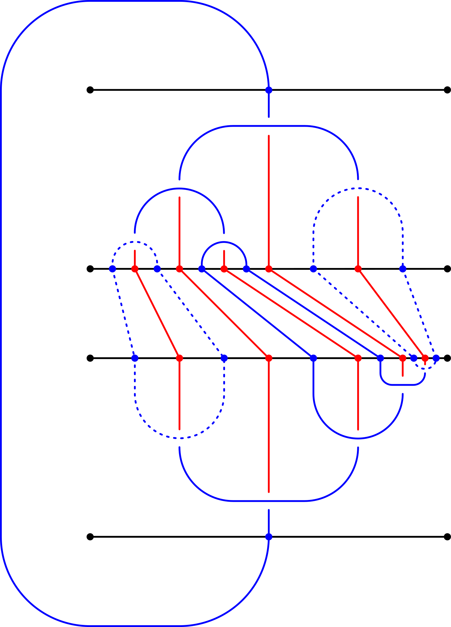
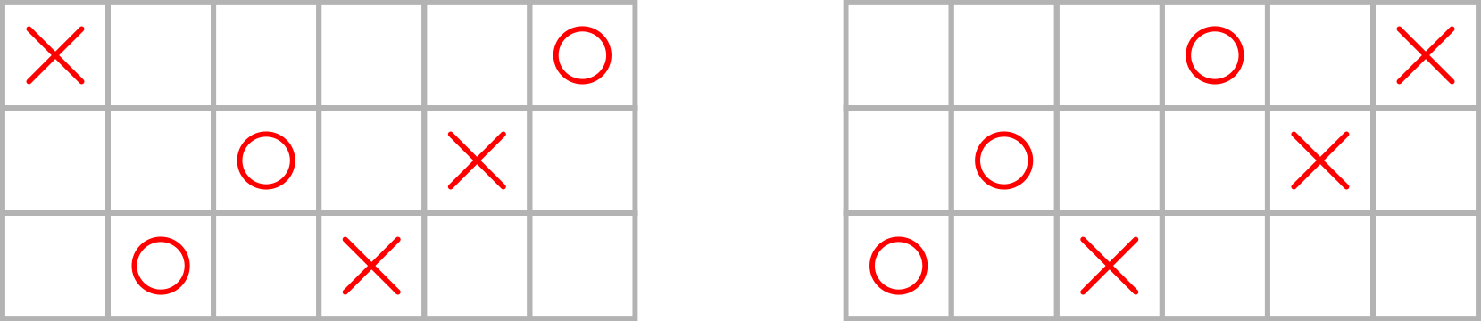
Let’s observe the pair of half grid diagrams in Figure 22. First, we try to write down their symmetric representations and (simply denoted as and ). Take as an example, for odd inputs, is the column index of in the row, so . For even inputs, is the column index of in the row, so . We can similarly write down . The result is
Notice that is not a compatible pair, because the first column of contains an , but the first column of contains an . In the language of representation representation, is odd, but is even.
To make sure that is a compatible pair, we just need to require that and have the same parity for any . An equivalent condition is that as two sets. Or, as two sets.
Next, we will study the link group given by a pair of half grid diagrams. Since the link group is independent of the orientation of the link, it is natural to introduce an unoriented grid diagram and an associated unoriented link.
Definition 5.9.
An unoriented grid diagram is an grid of squares, each of which is either empty or contains a marking . We require that in each row and column there are exactly two nonempty squares.
To distinguish (oriented) grid diagrams and unoriented grid diagrams, in the rest of this section we will denote oriented grid diagram as .
Any unoriented grid diagram has an associated unoriented link as follows.
Definition 5.10.
Let be an unoriented grid diagram. The unoriented link associated to is obtained by connecting two ’s in each row and connecting two ’s in each column, such that horizontal segments are always above vertical segments.
Remark 5.11.
Given an oriented grid diagram , we can replace every and with , to obtain an unoriented grid diagram . Conversely, given an unoriented diagram diagram and associated unoriented link , we can always manually replace each with an or an , so that the resulting diagram can give any orientation on . The procedure is shown as follows.
Start with an arbitrary in an arbitrary link component of , replace it with , then it will automatically specify an and an on any other on this component, to make sure that each row and each column has exactly one and exactly one . We repeat this procedure on all link components of to obtain an oriented grid diagram , which gives an orientation on . To get other orientations, we just need to change the orientations of some link components by flipping all of ’s and ’s on those components.
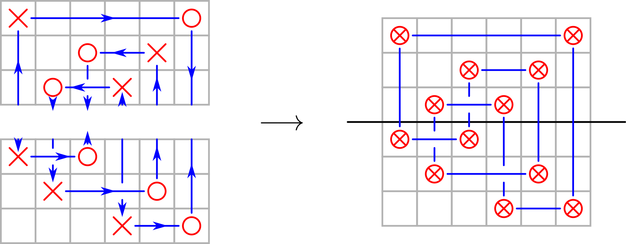
A nice thing of unoriented grid diagram is that even if we have two non-compatible half grid diagrams and , we still have an unoriented grid diagram by replacing every and in and by , then stacking over (see Figure 23 for an example). If we regard and as unoriented tangles, then we have . Furthermore, unoriented links and are mirrors of each other.
Definition 5.12.
An unoriented link is said to be half grid presentable if there exists a pair of (not necessarily compatible) half grid diagrams and such that as unoriented links, and we call a half grid representative of .
Proposition 5.13.
Every unoriented link is half grid presentable.
Proof.
Suppose is an unoriented link, we give it an arbitrary orientation and denoted the resulting oriented link as . By Theorem 1.10, there exists a pair of compatible half grid diagrams and such that as oriented links. Then as unoriented links. ∎
To prove Theorem 1.17, we first recall how to give a presentation of link group for some grid diagram .
Lemma 5.14.
[11, Lemma 3.5.1] The link group of has a presentation , called a grid presentation of link group. The generators correspond to the vertical segments in (connecting an and an in a column). The relations correspond to the horizontal lines separating the rows. The relation is the product of the generators corresponding to those vertical segments of the link diagram that meet the horizontal line, in the order they are encountered from left to right.
Note that link group is independent of link orientations, so we can replace the oriented grid diagram in Lemma 5.14 by unoriented grid diagram . See Figure 24(a) for an example of grid presentation of ’s link group.
Now we are ready to prove Theorem 1.17.
Proof of Theorem 1.17.
Let’s first prove that given any link, its link group has a half grid presentation (1.3). Since the link group does not depend on the orientation of link, we can start with an unoriented link . By Proposition 5.13, there exists a pair of half grid diagrams and such that .
Then we claim that the presentation of link group of given by Lemma 5.14 is the wanted half grid presentation. First, we index the horizontal line in the grid diagram from bottom to top with to (so the middle lines is the one). Observe that the horizontal line intersects with all vertical segments (see Figure 24(b) for an example), so we have
Other relations can be divided into two pieces and corresponding to and respectively. By the symmetric group representation given by Theorem 1.16, can be represented by some , where the and in the row of are exactly in the and columns. Observe that in the unoriented grid diagram , the horizontal line intersects with all vertical segments except the one and the one, because the and the on the first row of are below the horizontal line of . Then we take away and from to obtain . In general, we take away and from to obtain . This argument works similarly for . In conclusion, we have
We put relations together to get the half grid presentation of link group.
Conversely, suppose we have a group with a half grid presentation (1.3), for some positive integer and two elements , in . By Theorem 1.16, there is a pair of half grid diagrams and corresponding to and respectively. Notice that is not necessarily compatible, but we still have an unoriented grid diagram . Let be the unoriented link , then by previous discussion we conclude that the link group of has a presentation exactly same as the given half grid presentation of . So is indeed a link group. ∎
5.2.2 Half grid diagram and classical link invariants
In this subsection we will first prove Theorem 1.13. The result follows directly from the construction assigning a canonical Seifert surface to an oriented Thompson link diagram introduced by Jones in [6].
Given an s.d. partition pair , the signed regions in Figure 13(a) give a surface bounding . Furthermore, the and signs represent local orientations of the surface. Suppose that represents an element in , then implies that is orientable. Let it be the canonical Seifert surface of .

Now we are ready to see the Proof of Theorem 1.13
Proof of Theorem 1.13.
Suppose has , let be a compatible s.d. n-partition pair such that .Then there are total crossing in such diagram, and by the construction of Seifert surface discussed above it’s easy to see after we cut out the surface at the intersection points the surface decomposed into disks. In other words, the Seifert surface is obtained by attaching 1-handle to disks, so . Thus , which implies when has one component . ∎
Before we give proof of Theorem 1.15, let’s first recall the definition of minimal grid number of oriented link. Suppose is an oriented link. The minimal grid number of is defined to be the minimal number such that there exists an grid diagram satisfying . The minimal grid number of is denoted as .
Note that is independent of the orientation of , because we can always flip some ’s and ’s in to obtain any other orientation of . It is natural to define minimal grid number of unoriented link .
Definition 5.16.
Let be an unoriented link. The minimal grid number of is defined to be the minimal number such that there exists an unoriented grid diagram satisfying . The minimal grid number of is denoted as .
It’s easy to see that , where has an arbitrary orientation on .
Next, let’s see an unoriented version of Theorem 4.10.
Proposition 5.17.
Suppose that is any s.d. -partition pair (not necessarily compatible), then as unoriented links.
Proof.
Now Theorem 1.15 follows easily.
Appendix A Group of fractions
Let be a small category with the following 3 properties.
-
1.
(Unit) There is an element with for all .
-
2.
(Stabilization) Let . Then for each there are morphisms and with .
-
3.
(Cancellation) If for then .
Then becomes a directed set if we define given for some morphism .
Suppose that is another category and is a functor. For any , we let . If and , we define sending to . Then is a direct system. Notice that the cancellation axiom implies that is unique, and the stabilization axiom implies that for any there exists some such that and .
Let . There is bijection from to , sending to , and its inverse sends back to .
The inverse limit of the direct system is defined to be , where and are equivalent if there exists such that . In other words, there exist morphisms in such that and .
Correspondingly, there is an equivalence relation on such that if there exists morphisms in such that . Then
as sets. We don’t distinguish them from now on.
Let be the identity functor , then , and if there exists morphisms in such that . Given , we know there exist morphisms such that , then we define
This is a well-defined group structure on , and this group is called the group of fractions of , denoted as .
Now we define the category of forests to recover Thompson group as a group of fractions.
Definition A.1.
The category has objects positive numbers, with morphisms from to defined to be -forests. Compositions are concatenations of forests.
We can check that satisfies properties 1-3, and we have [7, Proposition 2.2.1]. To recover oriented Thompson group as a group of fractions, we need to consider signed forests instead.
Definition A.2.
The category has objects -signs, with morphisms from to defined to be signed forests (forests with signing rules shown in Figure 12(a)) inducing on the top and on bottom. Compositions are concatenations of signed forests.
also satisfies properties 1-3. Especially, let the unit of be the -sign . Then we have [2, Proposition 3.6]. Notice that each element in is a pair of signed trees from the -sign to , where the targets are the -signs induced by and respectively. So the definition of as a group of fractions coincides with Definition 3.9.
References
- [1] Valeriano Aiello. On the Alexander theorem for the oriented Thompson group . Algebr. Geom. Topol., 20(1):429–438, 2020.
- [2] Valeriano Aiello, Roberto Conti, and Vaughan F. R. Jones. The Homflypt polynomial and the oriented Thompson group. Quantum Topol., 9(3):461–472, 2018.
- [3] J. W. Cannon, W. J. Floyd, and W. R. Parry. Introductory notes on Richard Thompson’s groups. Enseign. Math. (2), 42(3-4):215–256, 1996.
- [4] Jean-Marie Droz and Emmanuel Wagner. Grid diagrams and Khovanov homology. Algebr. Geom. Topol., 9(3):1275–1297, 2009.
- [5] John B. Etnyre. Legendrian and transversal knots. In Handbook of knot theory, pages 105–185. Elsevier B. V., Amsterdam, 2005.
- [6] Vaughan F. R. Jones. Some unitary representations of Thompson’s groups and . J. Comb. Algebra, 1(1):1–44, 2017.
- [7] Vaughan F. R. Jones. A no-go theorem for the continuum limit of a periodic quantum spin chain. Comm. Math. Phys., 357(1):295–317, 2018.
- [8] Robert Lipshitz, Peter S. Ozsváth, and Dylan P. Thurston. Bordered Heegaard Floer homology. Mem. Amer. Math. Soc., 254(1216):viii+279, 2018.
- [9] Ciprian Manolescu, Peter Ozsváth, and Sucharit Sarkar. A combinatorial description of knot Floer homology. Ann. of Math. (2), 169(2):633–660, 2009.
- [10] Lenhard Ng. On arc index and maximal Thurston-Bennequin number. J. Knot Theory Ramifications, 21(4):1250031, 11, 2012.
- [11] Peter S. Ozsváth, András I. Stipsicz, and Zoltán Szabó. Grid homology for knots and links, volume 208 of Mathematical Surveys and Monographs. American Mathematical Society, Providence, RI, 2015.
- [12] Peter S. Ozsváth and Zoltán Szabó. Algebras with matchings and knot floer homology. preprint, 2019.
- [13] Peter S. Ozsváth and Zoltán Szabó. The pong algebra. preprint, 2022.
- [14] Olga Plamenevskaya. Bounds for the Thurston-Bennequin number from Floer homology. Algebr. Geom. Topol., 4:399–406, 2004.
- [15] Lawrence P. Roberts. A type structure in Khovanov homology. Algebr. Geom. Topol., 16(6):3653–3719, 2016.
- [16] Lawrence P. Roberts. A type structure in Khovanov homology. Adv. Math., 293:81–145, 2016.