Flexora: Flexible Low Rank Adaptation for Large Language Models

Abstract

Large Language Models (LLMs) are driving advancements in artificial intelligence by increasing the scale of model parameters, which has significantly enhanced generalization ability and unlocked new capabilities in practice. However, their performance in specific downstream tasks is usually hindered by their knowledge boundaries on these tasks. Thus, fine-tuning techniques, especially the widely used Low-Rank Adaptation (LoRA) method, have been introduced to expand the boundaries on these tasks, whereas LoRA would underperform on certain tasks owing to its potential overfitting on these tasks. To overcome this overfitting and improve the performance of LoRA, we propose the flexible low rank adaptation (Flexora) method to automatically and flexibly select the most important layers needing to be fine-tuned to achieve the best performance on different downstream tasks. Specifically, Flexora firstly frames this layer selection problem as a well-defined hyperparameter optimization (HPO) problem, then addresses it using the unrolled differentiation (UD) method, and finally selects the most useful layers based on the optimized hyperparameters. Our extensive experiments on many pre-trained models and natural language tasks show that Flexora is able to consistently improve over the existing baselines, indicating the effectiveness of our Flexora in practice. We additionally provide insightful theoretical results and many ablation studies to deliver a comprehensive understanding of our Flexora.

1 Introduction

The emergence of large language models (LLMs) (Zhao et al. 2023; Xu et al. 2023) has introduced significant computational demands (Touvron et al. 2023), characterized by extensive parameter sets and robust functionalities (Wei et al. 2022), necessitating substantial training resources. Consequently, parameter-efficient fine-tuning (PEFT) methods (Li and Liang 2021; Lester, Al-Rfou, and Constant 2021) have become increasingly popular. Among these, low-rank adaptation (LoRA) (Hu et al. 2021) is especially noteworthy. LoRA freezes pre-trained parameters and introduces auxiliary trainable parameters $\Delta\bm{W}$ at each layer, markedly reducing training costs while achieving impressive results. However, fine-tuning LLMs using LoRA still encounters challenges such as an excessive number of fine-tuning parameters and a tendency toward model overfitting, leading to suboptimal performance. Recently, researchers have proposed various methods to enhance LoRA. For example, AdaLoRA (Zhang et al. 2023b) employs singular value decomposition (SVD) to prune less critical singular values, while DoRA (Mao et al. 2024a) dynamically reduces high-rank LoRA layers into structured single-rank components. Additionally, techniques such as dropout (Lin et al. 2024) and novel regularization strategy (Mao et al. 2024b) have been proposed to address overfitting. Despite these improvements, several limitations persist. Performance is often comparable to or lower than that of LoRA, and these methods do not automatically tune hyperparameters to achieve optimality, nor do they offer flexibility. Therefore, there is a pressing need for an algorithm that delivers good performance, enables automatic selection, and supports flexible training, which we have developed.

Hyperparameter optimization (HPO) is a fundamental problem in the field of machine learning (Liu, Simonyan, and Yang 2019a; Franceschi et al. 2018; Ren et al. 2019; Guo et al. 2020). The goal of HPO is to identify hyperparameter-hypothesis pairs that optimize the expected risk of test samples drawn from an unknown distribution. This involves solving two nested optimization problems: the inner problem focuses on optimizing the hypothesis on the training set for a specified hyperparameter configuration, while the outer problem aims to find hyperparameters that minimize the validation error. In recent years, unfolded differentiation (UD) algorithms have emerged as the mainstream solution for HPO due to their potential to adjust a large number of hyperparameters (Franceschi et al. 2017; Fu et al. 2016; Maclaurin, Duvenaud, and Adams 2015; Shaban et al. 2019). Inspired by HPO, we consider each layer of an LLM as a hypothesis, facilitating a layer-wise analysis of LLMs. Driven by the desire for a deeper understanding of LLMs, we have undertaken this work.

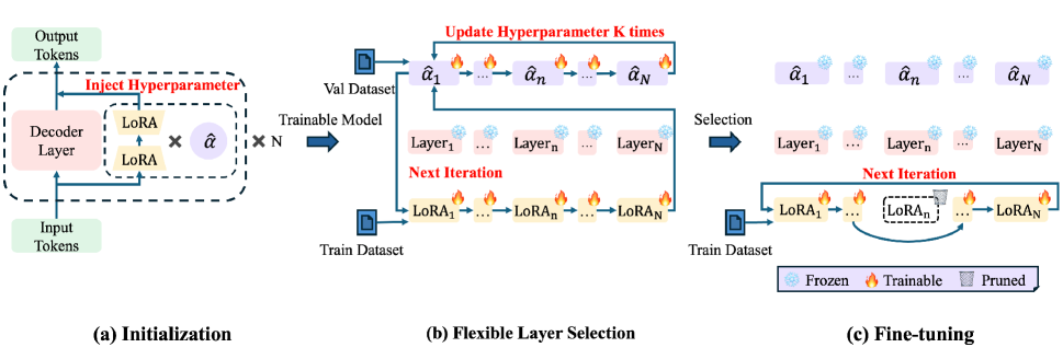
Figure 1: An overview of Flexora: An overview of our method: (a) Initialization of the hyperparameters $\widehat{\alpha}$ and their integration with the LoRA parameters to produce the Trainable Model. (b)Simultaneous training of the LoRA parameters and hyperparameters $\widehat{\alpha}$ using different datasets, leading to the minimization of empirical risk for both validation and training datasets. The hyperparameter vector $\widehat{\alpha}$ is then outputted and ranked based on the magnitude of each hyperparameter. (c) Flexible selection of the number of layers to be trained, denoted by “Selection”, where layers ranked higher are activated for training, while the remaining layers are kept frozen.

In this paper, we introduce a novel method, Flexora, designed to address the overfitting in LoRA by automatically and flexibly selecting the most critical layers for fine-tuning, as illustrated in Figure 1. To achieve this, we frame the layer selection problem as an HPO task and employ the UD method to solve it. More specifically, during the initialization stage, Flexora injects the defined hyperparameters into the LoRA parameters, producing a PEFT model ready for training. In the flexible layer selection stage, described in Sec. 4.1, the UD method optimizes this hyperparameter problem. Finally, in the fine-tuning stage, detailed in Sec. 4.2, Flexora uses the optimized hyperparameters to identify the layers that contribute most to downstream tasks for targeted fine-tuning. By restricting backpropagation and parameter updates to these selected layers, Flexora significantly reduces computational overhead. Empirical results demonstrate that Flexora effectively reduces unimportant LoRA parameters, suppresses model overfitting, and enhances performance. In summary, our contributions are as follows:

• We introduce Flexora to improve LoRA by automatically and flexibly selecting the most important layers for LoRA fine-tuning.

• We frame the layer selection problem as an HPO task and solve it effectively and efficiently using the UD method.

• We validate the effectiveness of our Flexora through extensive experiments on various LLMs and tasks, showing significant improvements over existing LoRA variants.

• We provide theoretical explanations for our experimental results, offering insights into the mechanisms behind the performance improvements achieved by Flexora.

2 Related Work

2.1 Low-Rank Adaptation (LoRA)

In recent years, low-rank adaptation (LoRA) methods have gained widespread adoption to reduce the number of training parameters while fine-tuning large language models (LLMs) for specific applications. However, LoRA frequently suffers from overfitting, which results in poor performance on downstream tasks. To address this issue, researchers have developed various methods to alleviate overfitting by reducing training parameters. Wu et al. (2024) found that training all LoRA parameters may lead to overfitting, and proposed LoRA-SP, which randomly freezes half of the LoRA parameters during fine-tuning, thus effectively alleviating overfitting. Zhang et al. (2023a) noted that the down-projection weights in LoRA might lead to overfitting, and introduced LoRA-FA, which freezes the down-projection weights and only updates the up-projection weights, thereby enhancing the performance. Zhou et al. (2024) proposed LoRA-drop, which prunes less important parameters based on layer output analysis, thus enhancing the generalization ability of the model. In contrast, Zhang et al. (2024) investigated the interaction between LoRA parameters and the original LLM and proposed LoRAPrune. This method jointly prunes parts of the LoRA matrix and parts of the LLM parameters based on the gradient of LoRA to further reduce overfitting. In addition, LoRAShear (Chen et al. 2023) introduces a knowledge-based structured pruning method that reduces the computational cost while retaining essential knowledge, thus reducing overfitting and enhancing generalization performance.

Unfortunately, these methods usually (a) require significant manpower in an algorithm or configuration design, (b) struggle to yield adaptive policies across different downstream tasks, and (c) are often too complex (i.e., parameter-level policies) to be applied in practice. In contrast, in this paper, we introduce Flexora, a framework that aims to flexibly fine-tune LoRA across various downstream tasks using an automated yet simple layer-level policy.

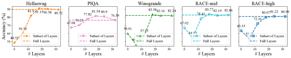
Figure 2: This figure depicts the relationship between the number of fine-tuning layers and model accuracy across four distinct datasets: Hellaswag, PIQA, Winogrande, and RACE, with the latter including two separate tasks, RACE-mid and RACE-high, which vary in difficulty. Each sub-figure is dedicated to one of these datasets. The horizontal axis quantifies the number of fine-tuning layers, ranging from 0 to 32. This scale includes the base model with 0 layers, and scenarios where 6, 12, 18, 24, and 32 layers are randomly fine-tuned, with the full 32 layers corresponding to the LoRA configuration. The vertical axis measures model accuracy, expressed as a percentage.

2.2 Hyperparameter Optimization (HPO)

HPO is widely applied across various domains. Specifically, in the domain of neural architecture search, Liu, Simonyan, and Yang (2019b) conceptualizes the coefficients defining the network architecture as hyperparameters. In the domains of feature learning, Guo et al. (2020) considers feature extractors as hyperparameters. In the field of data science, (Olson et al. 2016) employs hyperparameters as weights to measure the importance of data. By minimizing the validation loss over these hyperparameters, the optimal variables, e.g., the architectures in (Liu, Simonyan, and Yang 2019b), the features in (Guo et al. 2020), and the data in (Olson et al. 2016), are identified, leading to superior performance in their respective domains.

Drawing inspiration from these works, we initially formulated the layer selection in the LoRA method as an HPO problem. This involves optimizing hyperparameters to quantify the contributions of different layers, aiming to achieve optimal performance on downstream tasks and thereby select the most crucial layers for fine-tuning. This formulation subsequently led to the development of our algorithm (Flexora).

3 Preliminaries

In this section, we first provide empirical insights showing that layer selection is crucial for improved performance of LLMs in Sec. 3.1, and then frame the layer selection problem as a well-defined HPO problem in Sec. 3.2.

3.1 Empirical Insights

To investigate the relationship between the number of fine-tuning layers and overall performance, we conducted a preliminary study on Llama3-8B. The results, presented in Figure 2, indicate that while increasing the number of fine-tuning layers generally enhances model performance, there exists a critical threshold beyond which additional fine-tuning leads to overfitting and a subsequent decline in performance. Therefore, fine-tuning a subset of LoRA layers emerges as a natural strategy to minimize overfitting and enhance LoRA performance, aligning with numerous empirical findings. For instance, Zhu et al. (2023) employed a randomized and structured pruning approach on the original LLM pre-trained parameters and LoRA parameters of layers, training only the remaining subset of LoRA, and achieved favorable outcomes. Similarly, Zhou et al. (2024) analyzed the output values of LoRA elements across different layers and utilized output value pruning to reduce overfitting, thus improving performance by training a selected subset of layers. Additionally, Chen et al. (2023) highlighted that different layers encapsulate different types of knowledge, and pruning irrelevant layers can significantly enhance model performance on downstream tasks. In summary, fine-tuning a subset of LoRA layers offers several advantages: fewer parameters, reduced memory consumption, shorter training times, diminished overfitting, and ultimately, enhanced model performance.

3.2 Problem Formulation

Inspired by the insights above, we aim to identify the most critical layers in LLM fine-tuning with LoRA to further improve generalization performance on varying downstream tasks. Formally, given a $N$-layer LLM with LoRA fine-tuning parameter $\theta$, let hyperparameter $\alpha\in\{0,1\}^{N}$ represent the selection results of LoRA fine-tuning layers with 1 indicating that a layer will be selected, and define the expected test error ${\mathcal{R}}^{\text{test}}(\theta,\alpha)\triangleq\mathbb{E}_{x\sim{\mathcal{D}}_{\text{test}}}\ell(x,\theta;\alpha)$ and the expected training error ${\mathcal{R}}^{\text{train}}(\theta,\alpha)\triangleq\mathbb{E}_{x\sim{\mathcal{D}}_{\text{train}}}\ell(x,\theta;\alpha)$. To select the most important LoRA fine-tuning layers in this LLM for its optimal fine-tuning performance on downstream tasks, we need to solve the following bilevel optimization problem:

$$\min_{\alpha\in\{0,1\}^{N}}{\mathcal{R}}^{\text{test}}(\theta^{*}(\alpha),\alpha)\,\,\text{s.t.}\,\,\theta^{*}(\alpha)=\operatorname*{arg\,min}_{\theta\in\mathbb{R}}{\mathcal{R}}^{\text{train}}(\theta,\alpha)\ .$$ (1)

Of note, this formulation serves as a standard form of HPO as demonstrated in Bao et al. (2021), where $\alpha$ is the hyperparameter. Consequently, we have framed the layer selection problem in LLM fine-tuning with LoRA as a well-defined HPO problem.

Unfortunately, it is typically infeasible to obtain the training (i.e., ${\mathcal{D}}_{\text{train}}$) and test (i.e., ${\mathcal{D}}_{\text{test}}$) distributions for this optimization. As a result, we commonly use the training dataset $S_{\text{train}}$ and validation dataset $S_{\text{val}}$ to approximate the training and test distributions respectively. Define the empirical validation error $\widehat{{\mathcal{R}}}^{\text{val}}(\theta,\alpha)\triangleq\mathbb{E}_{x\sim{\mathcal{S}}_{\text{val}}}\ell(x,\theta;\alpha)$ and the empirical training error $\widehat{{\mathcal{R}}}^{\text{train}}(\theta,\alpha)\triangleq\mathbb{E}_{x\sim{\mathcal{S}}_{\text{train}}}\ell(x,\theta;\alpha)$, we aim to solve the following HPO problem:

$$\min_{\alpha\in\{0,1\}^{N}}\widehat{{\mathcal{R}}}^{\text{val}}(\theta^{*}(\alpha),\alpha)\,\,\text{s.t.}\,\,\theta^{*}(\alpha)=\operatorname*{arg\,min}_{\theta\in\mathbb{R}}\widehat{{\mathcal{R}}}^{\text{train}}(\theta,\alpha)\ .$$ (2)

4 The Flexora Framework

This section outlines the methodology behind our proposed Flexora framework. As shown in Figure 1, our Flexora framework consists of two major stages: a flexible layer selection stage detailed in Sec. 4.1 and a fine-tuning stage of the selected LoRA layers detailed in Sec. 4.2.

Algorithm 1 The Flexora Framework

1:  Input: Number of hyperparameter upgrade per iteration $K$; Number of iteration $T$; initialization LoRA Adapter parameters $\hat{\theta}_{0}$ and hyperparameter $\hat{\alpha}_{0}$; learning rate scheme $\eta_{\alpha}$ and $\eta_{\theta}$

2:  Output: The layer importance vector $\hat{\alpha}_{ud}$

3:  for $t=0$ to $T-1$ do

4:     $\hat{\theta}_{t+1}\leftarrow\hat{\theta}_{t}-\eta_{\theta,t+1}\nabla_{\theta}\widehat{{\mathcal{R}}}^{\text{train}}(\theta,\hat{\alpha}_{t})|_{\theta=\hat{\theta}_{t}}$

5:     for $k=0$ to $K-1$ do

6:        $\hat{\alpha}_{k+1}\leftarrow\hat{\alpha}_{k}-\eta_{\alpha,k+1}\nabla_{\alpha}\widehat{{\mathcal{R}}}^{\text{val}}(\hat{\theta}_{t+1}(\alpha),\alpha)|_{\alpha=\hat{\alpha}_{k}}$

7:     end for

8:  end for

9:  return $\hat{\alpha}_{ud}$

4.1 Flexible Layer Selection Stage

Relaxation and Computation.

Due to the difficulty of optimizing the discrete layer selection hyperparameter $\alpha=(\alpha_{1},\cdots,\alpha_{N})$ directly, we relax it to the continuous counterpart $\widehat{\alpha}=(\widehat{\alpha}_{1},\cdots,\widehat{\alpha}_{N})$, with each $\widehat{\alpha}_{i}$ defined as

$$\widehat{\alpha}_{i}=\frac{\exp{(\alpha_{i}})}{\sum_{i\in[N]}\exp{(\alpha_{i}})}N\ .$$ (3)

where $\alpha$ is initialized with zeros, and the constant scale $N$ is applied to ensure that the initialized $\widehat{\alpha}$ is equivalent to the selection of all LoRA layers. The specific computation involving this hyperparameter is as follows:

$$h_{i}=W_{0}z_{i}+\widehat{\alpha_{i}}B_{i}A_{i}z_{i}\ .$$ (4)

Therefore, if $\widehat{\alpha_{i}}$ is close to zero, it degenerates to the standard computation in the original LLM, indicating that LoRA is not required by this layer. Meanwhile, if $\widehat{\alpha_{i}}$ is larger, intuitively, this layer requires LoRA more significantly for better performance.

Table 1: Comparison of accuracy across various common sense reasoning tasks using the Llama3-8B. The specific experimental configuration of the baseline is detailed in Appendix B. Here, “Pre-trained” refers to directly using the pre-trained (i.e., base) model for reasoning, “Full FT” denotes full parameter fine-tuning, “LLaMA Pro” indicates that the layers selected are consistent with Flexora, and “Random (Greedy)” represents the best result from randomly selecting layers.

Methods	Hellaswag	PIQA	Winogrande	RACE-mid	RACE-high	Average
Pre-trained	48.55	67.08	59.91	67.02	63.35	61.18
Full FT	90.53	79.32	81.16	81.92	79.36	82.46
LLaMA Pro	90.03	76.23	80.32	82.68	80.96	82.04
LoRA	89.72	76.39	82.24	82.86	80.99	83.04
QLoRA	88.81	76.19	81.42	82.01	80.16	81.72
OLoRA	91.32	80.69	83.01	83.65	77.66	83.27
LoRA+	90.62	77.92	83.06	83.69	81.80	83.42
GaLore	90.42	77.56	81.36	81.43	79.68	82.09
PiSSA	91.33	77.77	83.72	84.35	82.15	83.86
ROSA	88.69	77.23	81.65	81.52	80.06	81.83
VeRA	90.98	78.63	83.64	83.55	78.84	83.13
LoRAPrune (Ratio = 0.5)	88.42	77.12	81.23	82.96	80.42	82.03
AdaLoRA ($r_{0}=4$)	90.17	80.20	77.19	83.15	77.93	81.73
LoRA-drop	91.86	77.91	76.46	77.30	75.24	79.75
Random (Greedy)	91.15	81.54	83.58	83.77	81.22	84.25
Flexora	93.62	85.91	85.79	84.61	82.36	86.46

Optimization.

To find the most important layers for fine-tuning LLMs on downstream tasks, we need to solve the HPO problem defined by Equation 2 in Section 3.2. To solve it, we will employ the UD algorithm. Specifically, we define $\operatorname*{arg\,min}_{\theta\in\mathbb{R}}\widehat{{\mathcal{R}}}^{\text{train}}(\theta,\alpha)$ as the inner layer optimization, where the LoRA parameter $\theta$ is updated. Similarly, we define $\operatorname*{arg\,min}_{\alpha\in\{0,1\}^{N}}\widehat{{\mathcal{R}}}^{\text{val}}(\theta^{*}(\alpha),\alpha)$ as the outer layer optimization, where the hyperparameter $\alpha$ is updated based on the results of the inner layer optimization.

According to the aforementioned explanation, our primary optimization target is the hyperparameter $\alpha$. In practice, we use Equation 3 to convert the hyperparameter $\alpha$ into $\widehat{\alpha}$, which guides the layer selection at each step. As illustrated in Figure 1a, we initially set $\alpha$ to zeros and inject the hyperparameter into all LoRA parameters. Next, as illustrated in Figure 1b, we conduct inner layer training optimization for all layers and retain all computational graphs for subsequent outer layer updates. It is crucial to note that the computational graph is differentiable with respect to the hyperparameter $\widehat{\alpha}$. Subsequently, we use the updated parameters $\theta$ and computational graphs to conduct outer layer training $K$ times. Each outer layer training iteration randomly selects batch data from the validation dataset for optimization. This process is formally described by Alg. 1, under the assumption that $\alpha$ and $\theta$ are independent of $S_{\text{val}}$ and $S_{\text{train}}$. When fine-tuning large language models (LLMs), the substantial sizes of $S_{\text{val}}$ and $S_{\text{train}}$ make the gradient computation of Alg. 1 computationally infeasible, necessitating the use of stochastic gradient descent (SGD) for hyperparameter updates with a single outer layer update as follows:

$$\widehat{\alpha}_{k+1}\leftarrow\widehat{\alpha}_{k}-\eta_{\alpha}\nabla_{\alpha}\widehat{{\mathcal{R}}}_{\text{val}}(\hat{\theta}^{t}(\alpha),\alpha)|_{\alpha=\widehat{\alpha}_{k},data=\{d_{j}\}}$$ (5)

where $d_{j}$ is randomly selected from $S_{\text{val}}$. In subsequent epochs, we first apply Equation 4 to update the LoRA parameters of different layers based on the latest hyperparameters $\widehat{\alpha}$. Then, we continue the optimization starting from the updated LoRA parameters. After minimizing the validation metric $\widehat{{\mathcal{R}}}_{\text{val}}$, as shown in Equation 2, we will end the training process and obtain the optimal configuration of hyperparameters.

Selection Strategy.

Based on our formulation, we have the following proposition:

Proposition 1.

For any $T\geq 0$ and $K\geq 0$ in our Alg. 1, the following condition holds if $\alpha$ is initialized with zeros,

$$\sum_{i=1}^{N}\alpha_{i}=0\ .$$

Proof detailed in Appendix A.1.Based on the optimized $\alpha^{*}$, we automatically select the layers with $\alpha_{i}>0$ which has $\widehat{\alpha}_{i}>1$ to obtain the best performance. When resources are limited, we can flexibly choose the number of layers to fine-tune, optimizing performance within these constraints. Consequently, we only need to select the x layers with the largest $\widehat{\alpha}_{i}$. This approach allows for both automatic and flexible selection of the number and specific layers for tuning.

Table 2: Comparison of training time and training parameters, in which the green font denotes the reduction ratio. The experiments are conducted on a single NVIDIA A100 GPU using Llama3-8B. Here, the time metric represents the wallclock time required by the fine-tuning phase of LoRA and Flexora, excluding the layer selection phase.

Metrics	Method	Hellaswag	PIQA	Winogrande	RACE
Time (h)	LoRA	5.30	4.03	4.96	8.37
	Flexora	4.71 (11.1%)	3.87 (4.0%)	3.84 (22.6%)	7.46 (10.9%)
# Params (M)	LoRA	3.4	3.4	3.4	3.4
	Flexora	2.00 (41.2%)	1.70 (50.0%)	1.70 (50.0%)	1.70 (50.0%)

4.2 Fine-Tuning Stage

Since the LoRA parameters of all layers are updated alongside the hyperparameters during the flexible layer selection stage, direct deletion of LoRA parameters from any layer is not feasible, necessitating a dedicated fine-tuning stage. During the fine-tuning stage, as illustrated in Figure 1c, we freeze the unselected layers and retrain the LoRA parameters from scratch. This selective activation strategy ensures that the model focuses on fine-tuning the most critical layers, thus minimizing overfitting and optimizing performance for specific downstream tasks.

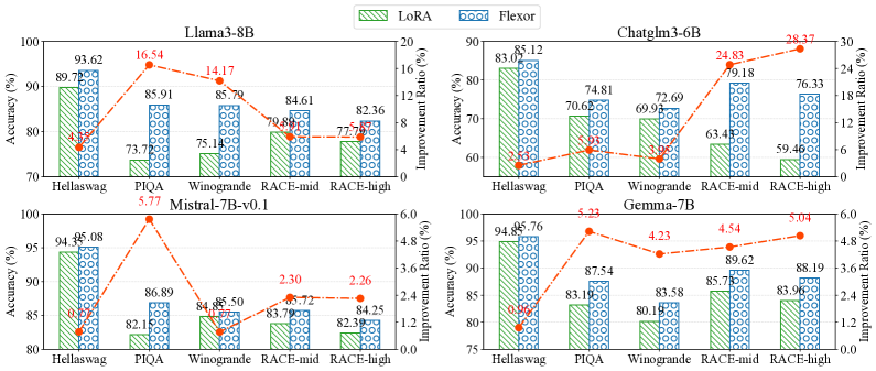
Figure 3: Comparison of the accuracy of different models (i.e., Llama-3-8B, ChatGLM3-6B, Mistral-7B-v0.1, and Gemma-7B) on different tasks. The bars with green diagonal stripes represent the accuracy achieved by LoRA, while the bars with blue circles represent the accuracy achieved by Flexora. It can be observed that Flexora generally outperforms LoRA in most tasks and models, indicating its effectiveness in improving model performance.

5 Empirical Results

In this section, we present a comprehensive set of experiments to assess the effectiveness and efficiency of our proposed Flexora method. We first describe the datasets and experimental setup. Next, we detail the main results and ablation studies.

5.1 Datasets and Setup

To evaluate the performance of our proposed Flexora method, we utilize several benchmark datasets, including Winogrande, RACE, PIQA, and Hellaswag, which collectively offer a comprehensive evaluation framework for various reasoning and comprehension tasks, with accuracy as the evaluation metric. Winogrande (Sakaguchi et al. 2019) evaluates commonsense reasoning using 44,000 questions, RACE (Lai et al. 2017) focuses on reading comprehension using nearly 100,000 questions, PIQA (Bisk et al. 2019) evaluates physics commonsense reasoning using more than 16,000 question-answer pairs, and Hellaswag (Zellers et al. 2019) tests commonsense natural language reasoning using 70,000 questions. In our experimental setup, we included 11 mainstream large-scale language models (LLMs), such as Llama3-8B (Meta 2024), Chatglm3-6B (GLM et al. 2024), Mistral-7B-v0.1 (Jiang et al. 2023), Gemma-7B (Team et al. 2024), and others. Flexora was developed using the Llama-factory (Zheng et al. 2024) framework and evaluated using the opencompass (Contributors 2023) framework. Detailed descriptions of data processing and experimental configurations can be found in the Appendix B. All experiments were performed on a single NVIDIA A100 GPU.

5.2 Main Results

In the main experiments, we assess the performance improvement and training efficiency of Flexora on Llama3-8B, with results presented in Table 1 (accuracy) and Table 2 (time and parameters). Baselines include pre-trained models, Full FT, LoRA, AdaLoRA, LoRA-drop, LoRAShear, and others. In particular, the experimental results with LoRAShear are detailed in Appendix C.3. The results indicate that Flexora outperforms all baselines. Compared to methods without LoRA, Flexora fine-tunes fewer parameters, thereby reducing overfitting and enhancing performance. When compared to methods that enhance LoRA, Flexora optimizes by considering the relationship between pre-trained parameters of each LLM layer and downstream tasks, achieving superior performance. Loss Detailed in Appendix C.6 Additionally, Flexora surpasses LoRA-drop, which always selects final layers, by identifying the most critical layers. Flexora also demonstrates strong generalization and scalability across different LLMs. Almost all LLMs can use Flexora to significantly improve performance with fewer fine-tuning parameters, as shown in Figure 3 and Appendix C.1

5.3 Ablation Studies

Ablation Study 1

In the first ablation experiment, we maintained the number of layers selected by Flexora unchanged but chose different layers for fine-tuning. The experimental results are shown in Table 3. The result underscores two key points: First, Flexora can precisely determine the number of layers for fine-tuning. Even when the specific fine-tuning layers are chosen at random, the results continue to outperform LoRA. The theoretical explanation for this result can be found in Sec. 6. Second, Flexora can automatically and flexibly select the specific layers for fine-tuning, targeting the most important layers to maximize performance and generalization. Detailed in Appendix C.5

Ablation Study 2

In the second ablation experiment, we manually determined the number of fine-tuning layers and contrasted Flexora with random selection. The results in Table 4 underscore the flexibility of Flexora, demonstrating that it can achieve optimal performance irrespective of the number of fine-tuning layers. The specific layers selected are shown in Table 12. An notable observation is that Flexora often selects the initial and final layers. An intuitive explanation is that the initial and final layers of a model have a significant impact on the data. The initial layer directly transforms the input into the feature space, while the final layer predicts the data in the form of labels, rendering them crucial. Additionally, for the same downstream task, the input to the initial layer remains consistent and closely aligned with the task, and the output of the final layer is also consistent. Focusing on optimizing these layers can enhance learning efficiency. This conclusion is corroborated by other studies. Chen et al. (2023) observed that the knowledge distribution in LLMs is primarily concentrated in the initial and final layers. Sharma, Ash, and Misra (2023) demonstrated that the loss gradient of the initial and final layers is steep, which benefits the model during training. Pan et al. (2024) found that the weight norm of the initial and final layers is hundreds of times greater than that of the intermediate layers, indicative of their heightened importance.

Table 3: Comparison of the accuracy of different randomly selected fine-tuning layers with the same number of fine-tuning layers. In this ablation study, we fixed the number of fine-tuning layers to match the number selected by Flexora, ensuring that the number of fine-tuning parameters remained constant while the layers were randomly selected for fine-tuning. The experiment demonstrates that, although random fine-tuning achieves commendable results given the same number of layers as determined by Flexora, Flexora consistently achieves the highest average accuracy.

Methods	Hellaswag	PIQA	Winogrande	RACE-mid	RACE-high	Average
Random 1	92.97	82.91	80.98	83.98	81.10	84.39
Random 2	93.11	80.79	76.09	85.45	81.16	83.32
Random 3	92.52	80.47	83.50	84.54	81.93	84.59
0-6[4pt/1pt] Random (Avg.)	92.87	81.39	80.19	84.66	81.40	84.10
Flexora	93.62	85.91	85.79	84.61	82.36	86.46

Table 4: Comparison of the accuracy of fine-tuning a subset of layers. In this ablation study, we standardized the number of layers to be fine-tuned and compared the performance of layers selected by Flexora against those selected randomly. The experimental results underscore the adaptability of Flexora. Regardless of the number of layers fine-tuned, Flexora consistently identifies the optimal layers, thereby achieving the maximum improvement with limited resources.

Methods	Hellaswag	PIQA	Winogrande	RACE-mid	RACE-high	Average
Random (6 Layers)	59.79	70.25	46.32	54.54	53.45	56.87
Flexora (First 6 Layers)	60.04 (+0.25)	77.20 (+6.95)	57.54 (+11.22)	69.71 (+15.17)	58.35 (+4.90)	64.57 (+7.70)
0-6[4pt/1pt] Random (12 Layers)	81.90	77.82	57.35	78.41	72.16	73.53
Flexora (First 12 Layers)	88.85 (+6.95)	79.71 (+1.89)	65.82 (+8.47)	79.42 (+1.01)	72.33 (+0.17)	77.23 (+3.70)
0-6[4pt/1pt] Random (18 Layers)	91.15	81.54	83.58	83.77	81.22	84.25
Flexora (First 18 Layers)	91.31 (+0.16)	82.21 (+0.67)	84.69 (+1.11)	84.07 (+0.30)	81.53 (+0.31)	84.76 (+0.51)
0-6[4pt/1pt] Random (24 Layers)	90.58	80.90	82.16	82.19	79.22	83.01
Flexora (First 24 Layers)	91.01 (+0.43)	81.21 (+0.31)	82.87 (+0.71)	83.53 (+1.34)	80.22 (+1.00)	83.77 (+0.76)

6 Theoretical Insights

In this section, we provide theoretical explanations for why Flexora (using only a subset of LoRA layers) can achieve excellent results. We first introduce Theorem 1 below, and then simplify LoRA layers as linear layers in multi-layer perceptron (MLP) to derive our Proposition 2, aiming to offer insights for this question.

Theorem 1.

(Hardt, Recht, and Singer 2016) Assume that $f(\cdot;z)\in[0,1]$ is an $L$-Lipschitz and $\beta$-smooth loss function for every sample z. Suppose that we run SGM for $T$ steps with monotonically non-increasing step sizes $\eta_{t}\leq c/t\ (t\in[T])$. In particular, omitting constant factors that depend on $\beta$, $c$, and $L$, we have

$${\mathcal{R}}^{\text{test}}(\theta,\eta)\leq\widehat{{\mathcal{R}}}^{\text{train}}(\theta,\eta)+\frac{T^{1-1/(\beta c+1)}}{m}\ .$$

Theorem 1 reveals that if all the conditions except for $\beta$ in Theorem 1 remain the same, a smaller smoothness $\beta$ will typically result in a smaller test error ${\mathcal{R}}^{\text{test}}(\theta,\eta)$, indicating a better generalization performance in practice. To show how the number of LoRA layers is related to this $\beta$, we then follow the practice in (Shu, Wang, and Cai 2020) to prove our Proposition 2 below.

Proposition 2.

For an $N$-layer linear multi-layer perceptron (MLP): $y^{(N)}\triangleq\prod_{j=1}^{N}W^{(j)}\bm{x}$ with MSE function $\ell\triangleq(y^{(N)}-y)^{2}/2$ where $y$ denotes the true label, let $\lambda^{(i)}=\left\|W^{(i)}\right\|$ for any $i\in[N]$, we then have.

$$\begin{split}&\left\|\frac{\partial\ell}{\partial W^{(i)}_{1}}-\frac{\partial\ell}{\partial W^{(i)}_{2}}\right\|\leq\left(\prod_{j=1,j\neq i}^{N}\lambda^{(j)}\right)^{2}\left\|\bm{x}\right\|^{2}\left\|W^{(i)}_{1}-W^{(i)}_{2}\right\|\ .\end{split}$$

The proof of Proposition 2 is detailed in Appendix A.3. given Proposition 2, the block-wise smoothness $\beta_{i}^{(N)}$ on layer $i\in[N]$ of an $N$-th layer MLP can be bounded by:

$$\begin{split}&\beta_{i}^{(N)}\ \leq\left(\prod_{j=1,j\neq i}^{N}\lambda^{(j)}\right)^{2}\left\|\bm{x}\right\|^{2}\ .\end{split}$$ (6)

From Equation 6, we can see that as the number of layers $N$ increases, the upper bound of $\beta_{i}^{(N)}$ will also be increasing as $\lambda^{(i)}>1$ for $i\in[N]$. Thus, shallow MLP of fewer layers are more likely to have smaller overall smoothness $\beta$. Thanks to this smaller overall smoothness $\beta$, shallow MLP of fewer layers are more likely to achieve a smaller generalization gap (i.e., the second term on the right-hand side of Theorem 1) than deep MLP with more layers. When the training error ${\mathcal{R}}^{\text{train}}(\theta,\eta)$ is the same, that is, both shallow and deep MLPs are fully trained to converge, the shallower MLP may have a lower test error ${\mathcal{R}}^{\text{test}}(\theta,\eta)$ and thus may exhibit better generalization performance on downstream tasks.

Now, we can answer the question posed at the beginning of this section. When Flexora is fine-tuned with a subset of LoRA layers, it theoretically transforms a network with a deeper architecture into one with a shallower architecture. When sufficiently trained to convergence, the aforementioned theory suggests that a network with a shallower architecture can exhibit better generalization and performance on downstream tasks. In summary, the reason Flexora achieves excellent results is that it makes the model more suitable for downstream tasks.

7 Conclusion and Future Work

In this study, we introduce Flexora, a method designed to enhance the efficiency and effectiveness of fine-tuning large language models (LLMs). Flexora automatically and flexibly selects the most critical layers for fine-tuning, addressing overfitting and enhancing performance by modeling layer selection as an HPO problem and employing UD to solve it. This targeted fine-tuning approach reduces computational overhead by updating only selected layers. Extensive experiments demonstrate Flexora reduces parameters, suppresses overfitting, and enhances performance, outperforming baseline methods. We also provide a theoretical explanation for these improvements.

Future work will focus on the following areas: (a) Exploring the relationship between individual layers of the LLM and their impact on downstream tasks to theoretically elucidate the role of each layer in reasoning processes. (b) Investigating optimal fine-tuning schemes for Flexora, inspired by its enhanced performance when integrated with various LoRA-enhanced algorithms, as demonstrated in Appendix C.2.

Reproducibility Checklist

This paper:

• Includes a conceptual outline and/or pseudocode description of AI methods introduced (yes)

• Clearly delineates statements that are opinions, hypothesis, and speculation from objective facts and results (yes)

• Provides well marked pedagogical references for less-familiare readers to gain background necessary to replicate the paper (yes)

Does this paper make theoretical contributions? (yes)

If yes, please complete the list below.

• All assumptions and restrictions are stated clearly and formally. (yes)

• All novel claims are stated formally (e.g., in theorem statements). (yes)

• Proofs of all novel claims are included. (yes)

• Proof sketches or intuitions are given for complex and/or novel results. (yes)

• Appropriate citations to theoretical tools used are given. (yes)

• All theoretical claims are demonstrated empirically to hold. (yes)

• All experimental code used to eliminate or disprove claims is included. (yes)

Does this paper rely on one or more datasets? (yes)

If yes, please complete the list below.

• A motivation is given for why the experiments are conducted on the selected datasets (yes)

• All novel datasets introduced in this paper are included in a data appendix. (no)

• All novel datasets introduced in this paper will be made publicly available upon publication of the paper with a license that allows free usage for research purposes. (no)

• All datasets drawn from the existing literature (potentially including authors’ own previously published work) are accompanied by appropriate citations. (yes)

• All datasets drawn from the existing literature (potentially including authors’ own previously published work) are publicly available. (yes)

• All datasets that are not publicly available are described in detail, with explanation why publicly available alternatives are not scientifically satisficing. (yes)

Does this paper include computational experiments? (yes)

If yes, please complete the list below.

• Any code required for pre-processing data is included in the appendix. (yes).

• All source code required for conducting and analyzing the experiments is included in a code appendix. (yes)

• All source code required for conducting and analyzing the experiments will be made publicly available upon publication of the paper with a license that allows free usage for research purposes. (yes)

• All source code implementing new methods have comments detailing the implementation, with references to the paper where each step comes from (yes)

• If an algorithm depends on randomness, then the method used for setting seeds is described in a way sufficient to allow replication of results. (yes)

• This paper specifies the computing infrastructure used for running experiments (hardware and software), including GPU/CPU models; amount of memory; operating system; names and versions of relevant software libraries and frameworks. (no)

• This paper formally describes evaluation metrics used and explains the motivation for choosing these metrics. (yes)

• This paper states the number of algorithm runs used to compute each reported result. (yes)

• Analysis of experiments goes beyond single-dimensional summaries of performance (e.g., average; median) to include measures of variation, confidence, or other distributional information. (yes)

• The significance of any improvement or decrease in performance is judged using appropriate statistical tests (e.g., Wilcoxon signed-rank). (yes)

• This paper lists all final (hyper-)parameters used for each model/algorithm in the paper’s experiments. (yes)

• This paper states the number and range of values tried per (hyper-) parameter during development of the paper, along with the criterion used for selecting the final parameter setting. (yes)

Appendix A Theorems and proofs

We first prove Proposition 1, then introduce the theorems proposed by Blair (1985) and Hardt, Recht, and Singer (2016), which reveal the properties of $\beta$-smooth, a necessary theoretical basis for proving Proposition 2. Finally, we prove Proposition 2.

A.1 Proof of proposition 1

The proof of Proposition 1 is expressed as follows:

Proof.

It is easy to verify that

$$\frac{\partial\widehat{\alpha}_{j}}{\partial\alpha_{i}}=\begin{cases}\widehat{\alpha}_{j}(1-\frac{1}{n}\widehat{\alpha}_{j}),&\text{if }j=i\\ -\frac{1}{n}\widehat{\alpha}_{j}\widehat{\alpha}_{i},&\text{if }j\neq i\end{cases}.$$

Therefore, given that $\sum_{i=1}^{n}\widehat{\alpha}_{i}=n$

$$\sum_{i=1}^{n}\frac{\partial\widehat{{\mathcal{R}}}^{\text{val}}}{\partial{\widehat{\alpha}_{j}}}\frac{\partial\widehat{\alpha}_{j}}{\partial\alpha_{i}} =\frac{\partial\widehat{{\mathcal{R}}}^{\text{val}}}{\partial{\widehat{\alpha}_{j}}}\left(\widehat{\alpha}_{j}-\frac{1}{n}\widehat{\alpha}^{2}_{j}-\frac{1}{n}\sum_{i=1,i\neq j}^{n}\widehat{\alpha}_{j}\widehat{\alpha}_{i}\right)$$

$$=\frac{\partial\widehat{{\mathcal{R}}}^{\text{val}}}{\partial{\widehat{\alpha}_{j}}}\left(\widehat{\alpha}_{j}-\frac{\widehat{\alpha}_{j}}{n}\sum_{i=1}^{n}\widehat{\alpha}_{i}\right)$$

$$=0\ .$$

When applying SGD to update $\alpha$, we have

$$\sum_{i=1}^{n}\alpha_{i}-\eta\sum_{i=1}^{n}\sum_{j=1}^{n}\frac{\partial\widehat{{\mathcal{R}}}^{\text{val}}}{\partial{\widehat{\alpha}_{j}}}\frac{\partial\widehat{\alpha}_{j}}{\partial\alpha_{i}}=\sum_{i=1}^{n}\alpha_{i}\ .$$

That is, the updated $\alpha$ shares the same summation as the one before the updates, which therefore concludes our proof. ∎

A.2 $\beta$-smooth

Definition 1.

$\beta$-smooth refers to the Lipschitz continuity of the gradient of the loss function, that is, for all $w$ and $w^{\prime}$:

$$\|\nabla f(w;z)-\nabla f(w^{\prime};z)\|\leq\beta\|w-w^{\prime}\|$$

where $\|\cdot\|$ denotes the norm of the vector, and $f(w;z)$ is the loss function with parameter $w$ for sample $z$.

Let $f_{\text{deep}}(w)$ and $f_{\text{shallow}}(w)$ be the loss functions for deep and shallow architectures, respectively. According to Definition 1, the relationship between $\beta_{\text{deep}}$ and $\beta_{\text{shallow}}$ illustrates the relationship between the generalization and performance of deep and shallow networks.

A.3 Proof of proposition 2

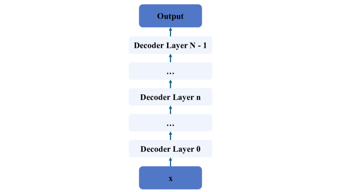
Figure 4: We present LLM as a hierarchical network. In this context, all parameters of a Decoder layer are represented as a weight matrix $W$ for subsequent analysis.

Abstract LLM into a layered network:(Shu, Wang, and Cai 2020) As shown in Figure 4, we abstract LLM into a hierarchical network, and the weight of each layer is represented by $W^{(i)}$. Figure 4 represents the general case. The output of the $i$-th layer network is:

$$\bm{y}=\prod_{j=1}^{n}W^{(j)}\bm{x}.$$ (7)

Gradient analysis: For the abstract network, represented in Equation 7. The gradient of the loss function $\ell$ with respect to the weight $W^{(i)}$ is:

$$\frac{\partial\ell}{\partial W^{(i)}} =\left(\prod_{j=i+1}^{n}W^{(j)}\right)\frac{\partial\ell}{\partial\bm{y}^{(i)}}\bm{x}\left(\prod_{j=1}^{i-1}W^{(j)}\right).$$ (8)

The proof of Proposition 2 is expressed as follows:

Proof.

For the abstract network, we begin with Definition 1:

$$\left\|\frac{\partial\ell}{\partial W^{(i)}_{1}}-\frac{\partial\ell}{\partial W^{(i)}_{2}}\right\|$$ (9)

$$=\left\|\left(\prod_{j=i+1}^{n}W^{(j)}\right)\left(\frac{\partial\ell}{\partial\bm{y}^{(i)}_{1}}-\frac{\partial\ell}{\partial\bm{y}^{(i)}_{2}}\right)\bm{x}\left(\prod_{j=1}^{i-1}W^{(j)}\right)\right\|.$$

Taking MSE Loss as an example, for one predictions $y^{(N)}$ and their corresponding true values $y$:

$$\ell\triangleq(\bm{y}^{(N)}-\bm{y})^{2}/2,$$ (10)

therefore:

$$\frac{\partial\ell}{\partial\bm{y}^{(i)}}=\left(\bm{y}^{(N)}-\bm{y}\right)\prod_{j=i+1}^{N}W^{(j)}.$$ (11)

We select the MSE loss function and calculat the $i$-th layer of N layers network, Substituting Equation 11 into Equation 9:

$$\left\|\frac{\partial\ell}{\partial W^{(i)}_{1}}-\frac{\partial\ell}{\partial W^{(i)}_{2}}\right\| =\left\|\left(\prod_{j=i+1}^{N}W^{(j)}\right)^{2}\left(\bm{y}^{(N)}_{1}-\bm{y}-\bm{y}^{(N)}_{2}+\bm{y}\right)\bm{x}\left(\prod_{j=1}^{i-1}W^{(j)}\right)\right\|$$ (12)

$$\leq\left(\frac{1}{\lambda^{(i)}}\left(\prod_{j=1}^{N}\lambda^{(j)}\right)\right)\left(\prod_{j=i+1}^{N}\lambda^{(j)}\right)\left\|\prod_{j=1}^{i-1}W^{(j)}\left(W^{(i)}_{1}-W^{(i)}_{2}\right){\bm{x}^{2}}\right\|$$

$$\leq\left(\prod_{j=1,j\neq i}^{N}\lambda^{(j)}\right)\left\|{\bm{x}^{2}}\right\|\left(\prod_{j=i+1}^{N}\lambda^{(j)}\right)\left(\prod_{j=1}^{i-1}\lambda^{(j)}\right)\left\|\left(W^{(i)}_{1}-W^{(i)}_{2}\right)\right\|$$

$$\leq\left(\prod_{j=1,j\neq i}^{N}\lambda^{(j)}\right)^{2}\left\|{\bm{x}^{2}}\right\|\left\|W^{(i)}_{1}-W^{(i)}_{2}\right\|.$$

∎

Appendix B Experimental setting

In the main experiment, we compared Flexora with the baseline. The datasets and experimental parameters are as follows:

B.1 Dataset

We added new templates to the original dataset to ensure the model could complete the required tasks and output formats. It is important to note that the added templates did not alter the original dataset, and special processing was performed for different LLMs. The specific examples are as follows:

B.2 Specific experimental parameters

Based on the Llama3-8B model configuration, several adjustments were made to optimize model performance. In the baseline model experiment, generation parameters were adjusted to ensure the correct output. In the LoRA experiment, adjustments to the generation parameters were retained, and LoRA-related parameters were adjusted. In the Flexora experiment, the size of the validation set was adjusted to control the time required to search for the optimal layer. In the AdaLoRA experiment, the initial rank size was modified to ensure that the fine-tuning parameters are consistent with Flexora. In the LoRA-drop experiment, the number of fine-tuning layers was set to be consistent with Flexora to ensure that the fine-tuning parameters are consistent. In the LoRAShear experiment, the pruning ratio was modified, where the parameter amount with a pruning ratio of 50% is consistent with Flexora. For specific experimental parameters, see the table 5.

Table 5: Detailed experimental parameters. This table lists the specific parameters we used in the experiments for various methods. These parameters include the target module of LoRA (Lora Target), the maximum sequence length (Max Length), the number of samples for supervised fine-tuning (SFT Samples), the learning rate (LR), the number of search samples (Search Samples), the initial rank (Init Rank), the target rank (Target Rank), and the ratio of pruning (Ratio). All other parameters not listed here remain consistent across all experiments.

Methods	LoRA Target	Max Length	SFT Samples	LR	Search Samples	Init Rank	Target Rank	Ratio
LoRA	q & v Proj	1024	20000	0.0001	-	-	-	-
Flexora	q & v Proj	1024	20000	0.0001	20000	-	-	-
AdaLoRA	q & v Proj	1024	20000	0.0001	-	4	8	-
LoRA-drop	q & v Proj	1024	20000	0.0001	20000	-	-	-
LoRAShear	q & v Proj	1024	20000	0.0001	20000	-	-	0.5
Dora	q & v Proj	1024	20000	0.0001	20000	-	-	-
rsLoRA	q & v Proj	1024	20000	0.0001	20000	-	-	-
LoRAPrune	q & v Proj	1024	20000	0.0001	20000	-	-	0.5

B.3 Other LLMs experimental parameters

In order to explore the versatility and scalability of Flexora, we conducted experiments on multiple different LLMs. The specific training parameters are shown in Table 6.

Table 6: Detailed LLM experiment parameters. This table provides a comprehensive overview of the specific parameters used for different large language models (LLMs) in our experiments. These parameters include the LoRA alpha value (LoRA Alpha), the dropout rate of LoRA (LoRA Dropout), the rank used in LoRA (LoRA Rank), and the target module of LoRA (LoRA Target). In addition, the table lists the specific templates used for each LLM, which are derived from Llama-factory (Template). For experiments involving different downstream tasks using the same model, all other parameters are kept consistent to ensure fair comparison and best performance.

LLM	LoRA Alpha	LoRA Dropout	LoRA Rank	LoRA Target	Tamplate (From Llama-factory)
Llama3	16	0	8	q & v Proj	llama3
Llama	16	0	8	q & v Proj	defult
Llama2	16	0	8	q & v Proj	llama2
chatglm3	16	0	8	query_key_value	chatglm3
Mistral-v0.1	16	0	8	q & v Proj	mistral
gemma	16	0	8	q & v Proj	gemma
zephyr	16	0	8	q & v Proj	zephyr
vicuna	16	0	8	q & v Proj	vicuna
xuanyuan	16	0	8	q & v Proj	xuanyuan
qwen1.5	16	0	8	q & v Proj	qwen
yi	16	0	8	q & v Proj	yi

Appendix C More results

C.1 The results of other LLMs experiment

Wide Applicability of Flexora.

According to the parameter settings in Table 6, the verification results for various LLMs are presented in Table 7. The selected LLMs include Llama3-8B, Llama-7B, Llama2-7B, ChatGLM3-6B, Mistral-7B-v0.1, Gemma-7B, Zephyr-7B-beta, Vicuna-7B-v1.5, XuanYuan-6B, Qwen1.5-7B, and Yi-6B. These models demonstrate unique characteristics in terms of training data, architecture design, and optimized training. First, the models utilize varied training data, leading to differences in data distribution. Additionally, some models have enhanced attention mechanisms: Mistral-7B-v0.1 employs grouped query attention (GQA) and sliding window attention (SWA), while ChatGLM3-6B features a special attention design to support tool calling and code execution capabilities. Activation functions vary across these models. Llama3-8B uses the SwiGLU activation function, inspired by the PaLM model, to improve performance and convergence speed, while ChatGLM3-6B uses the Swish activation function. Furthermore, differences in reasoning optimization and multilingual capabilities contribute to varied reasoning abilities across fields. The experimental result of each model is shown in Table 7, which presents the scores of each model on different downstream tasks after LoRA and Flexora fine-tuning. It should be noted that all models fine-tuned using LoRA will have a certain degree of overfitting, while Flexora can effectively identify and analyze unnecessary layers in specific downstream tasks and prune them to reduce model overfitting. After optimization by Flexora, these LLMs showed significant performance improvements on downstream tasks. In particular, models that originally performed poorly on some tasks, such as ChatGLM3-6B, experienced significant improvements, achieving more than a 15% increase on the RACE-mid and RACE-high tasks. This improvement is attributable to the key layer selection by Flexora and efficient model learning. In summary, Flexora is applicable across Transformer models of various structures, excels in diverse tasks, and effectively enhances areas where model capabilities are lacking.

Table 7: Detailed comparison of the accuracy of different LLMs. This table presents a comprehensive comparison of the accuracy results obtained by fine-tuning various mainstream Large Language Models (LLMs) using Flexora and LoRA methods. The accuracy metrics are reported across multiple benchmark datasets, including HellaSwag, PIQA, Winogrande, RACE-mid, and RACE-high. The average accuracy across all datasets is also provided. The exact values of accuracy improvements for each method, highlighted in red, indicate the performance gains achieved. For detailed experimental configurations, please refer to Appendix B.

Methods	Hellaswag	PIQA	Winogrande	RACE-mid	RACE-high	Average
Llama3-8B-LoRA	89.72	73.72	75.14	79.89	77.79	79.25
Llama3-8B-Flexora	93.62 (+3.90)	85.91 (+12.19)	85.79 (+10.65)	84.61 (+4.72)	82.36 (+4.57)	86.46 (+7.21)
Llama-7B-LoRA	76.10	69.80	67.01	75.69	70.81	71.88
Llama-7B-Flexora	85.28 (+9.18)	71.93 (+2.13)	74.11 (+7.10)	81.62 (+5.93)	78.62 (+7.81)	78.31 (+6.43)
Llama2-7B-LoRA	79.60	75.90	78.60	79.32	75.07	77.70
Llama2-7B-Flexora	90.89 (+11.29)	81.72 (+5.82)	82.85 (+4.25)	84.89 (+5.57)	83.19 (+8.12)	84.71 (+7.01)
Chatglm3-6B-LoRA	83.02	70.62	69.93	63.43	59.46	69.29
Chatglm3-6B-Flexora	85.12 (+2.10)	74.81 (+4.19)	72.69 (+2.76)	79.18 (+15.75)	76.33 (+16.87)	77.63 (+8.33)
Mistral-7B-v0.1-LoRA	94.35	82.15	84.85	83.79	82.39	85.51
Mistral-7B-v0.1-Flexora	95.08 (+0.73)	86.89 (+4.74)	85.50 (+0.65)	85.72 (+1.93)	84.25 (+1.86)	87.49 (+1.98)
Gemma-7B-LoRA	94.85	83.19	80.19	85.73	83.96	85.58
Gemma-7B-Flexora	95.76 (+0.91)	87.54 (+4.35)	83.58 (+3.39)	89.62 (+3.89)	88.19 (+4.23)	88.94 (+3.35)
Zephyr-7B-beta-LoRA	93.77	75.03	78.37	83.45	82.25	82.57
Zephyr-7B-beta-Flexora	95.05 (+1.28)	85.58 (+10.55)	84.95 (+6.58)	86.19 (+2.74)	84.30 (+2.05)	87.21 (+4.64)
Vicuna-7B-v1.5-LoRA	87.64	69.48	63.85	67.30	73.90	72.43
Vicuna-7B-v1.5-Flexora	90.43 (+2.79)	79.49 (+10.01)	76.06 (+12.21)	82.94 (+15.64)	81.90 (+8.00)	82.16 (+9.73)
XuanYuan-6B-LoRA	82.38	74.16	65.27	78.04	72.11	74.39
XuanYuan-6B-Flexora	88.41 (+6.03)	79.43 (+5.27)	73.40 (+8.13)	84.89 (+6.85)	80.70 (+8.59)	81.37 (+6.97)
Qwen1.5-7B-LoRA	91.75	75.03	78.14	87.59	81.36	82.77
Qwen1.5-7B-Flexora	91.96 (+0.21)	84.33 (+9.30)	80.69 (+2.55)	89.90 (+2.31)	87.08 (+5.72)	86.79 (+4.02)
Yi-6B-LoRA	89.46	78.29	76.01	80.02	85.13	81.78
Yi-6B-Flexora	92.24 (+2.78)	84.82 (+6.53)	84.96 (+8.95)	88.72 (+8.70)	86.91 (+1.78)	87.53 (+5.75)

C.2 The results of other LoRAs experiment

Strong Scalability of Flexora.

Recently, as emphasized in the Introduction 1, numerous LoRA improvement methods have been proposed, achieving excellent performance in specific fine-tuning tasks. In this section, the potential for combining Flexora with other emerging LoRA algorithms is explored. Two promising LoRA variants were selected from different approaches, each demonstrating impressive performance. Specifically, DoRA (Weight-Decomposed Low-Rank Adaptation) achieves low-rank adaptation through weight decomposition, and rsLoRA (Rank-Stabilized LoRA) addresses the slow training speed of traditional LoRA by introducing a rank-stabilized scaling factor when increasing rank. These methods primarily address the parameter overfitting problem within LoRA parameters but overlook the overall overfitting issue. These methods were innovatively combined with Flexora to first address the overall overfitting problem and then tackle the overfitting of the remaining LoRA parameters, resulting in notable performance improvements. The specific experimental results are shown in Table 8. The results indicate that Flexora integrates well with both DoRA and rsLoRA, effectively mitigating the overfitting problem of LLMs and improving performance with training on less than half of the parameters. The specific implementation entails replacing LoRA with DoRA or rsLoRA for inner layer optimization during the flexible layer selection stage, with the outer layer optimization remaining unchanged. These adjustments are achievable through straightforward modifications. The results demonstrate that Flexora exhibits strong scalability when combined with algorithms that enhance LoRA parameters, highlighting its significant potential.

Table 8: Detailed comparison of the accuracy of the combination of Flexora and different LoRA algorithms on Llama3-8B. This table presents a detailed comparison of the accuracy results obtained by integrating Flexora with various improved LoRA algorithms, including DoRA and rsLoRA, while maintaining other experimental settings constant. The accuracy metrics are reported across multiple benchmark datasets, including HellaSwag, PIQA, Winogrande, RACE-mid, and RACE-high, with the average accuracy across all datasets also provided. The results are compared against those obtained from direct fine-tuning without Flexora. The experimental findings indicate that the application of Flexora can significantly reduce model overfitting and enhance overall performance.

Methods	Hellaswag	PIQA	Winogrande	RACE-mid	RACE-high	Average
LoRA	89.72	76.39	82.24	85.86	80.99	83.04
Flexora (w/ LoRA)	93.62	85.91	85.79	84.61	82.36	86.46
rsLoRA	94.33	87.21	85.32	87.60	84.36	87.76
Flexora (w/ rsLoRA)	94.83	87.58	86.69	88.21	85.46	88.55
DoRA	93.62	85.75	84.77	86.77	83.39	86.86
Flexora (w/ DoRA)	94.10	86.05	86.32	87.12	84.45	87.61

C.3 Comparison with LoRAShear

Better Performance of Flexora.

In this section, the accuracy of Flexora is compared with that of LoRAShear across various datasets, with specific results presented in Table 9. Since LoRAShear is not open source and poses challenges for direct experimentation, the comparison relies on the experimental configurations and results reported in the LoRAShear paper. Notably, Flexora can freely adjust the selected layers according to the dataset, achieving an average pruning parameter rate of 50%. Consequently, under the same pruning rate, Flexora outperforms by 14% (Ratio = 0.5).Experiments have shown that under the same pruning rate, Flexora can achieve better performance.

Table 9: Detailed comparison of commonsense reasoning task accuracy. This table provides a comprehensive comparison of the accuracy results for various methods applied to common sense reasoning tasks, conducted on the Llama-7B model. The methods compared include the pre-trained model, LoRA, LoRAShear with different pruning ratios (0.5), and Flexora. The accuracy metrics are reported across multiple benchmark datasets, including BoolQ, PIQA, HellaSwag, Winogrande, ARC-e, ARC-c, and OBQA. The average accuracy across all datasets is also provided. The specific experimental configuration of the baseline is detailed in Appendix B. The “Ratio” column represents the ratio of parameter pruning in LoRAShear.

Methods	BoolQ	PIQA	HellaSwag	WinoGrande	ARC-e	ARC-c	OBQA	Average
Pre-trained	57.98	60.94	34.35	52.25	31.82	27.30	35.80	42.92
LoRA	67.76	69.80	76.10	67.01	67.21	35.23	38.60	60.24
LoRAShear (Ratio = 0.5)	63.40	72.15	49.83	56.40	49.45	34.31	35.86	51.63
Flexora	73.54	71.93	85.28	74.11	71.22	45.64	39.86	65.94

C.4 Different search sample

Flexibility of Flexora.

In Flexora, search time is managed by adjusting the maximum number of search samples (corresponding to the size of the validation dataset) to align with the requirements of the downstream task. In Table 10, we explore the relationship between different numbers of search samples, downstream task performance, and search time. For simpler datasets like Hellaswag and PIQA, a 10-minute search with 1,000 samples significantly improves performance. For more challenging tasks, at least 1 hour of search time is required for 5,000 samples. In more difficult tasks, using too few samples can prevent validation loss from converging. To optimize performance, it is recommended to dynamically adjust the number of search samples based on the convergence of the validation loss. In summary, for simpler downstream tasks, Flexora can be rapidly applied to reduce model overfitting significantly and enhance performance. For more challenging downstream tasks, Flexora balances performance and training resources by adjusting the number of search samples.

Table 10: Detailed analysis of the impact of different numbers of search samples on the Flexora accuracy of Llama3-8B. This table investigates how varying the number of search samples, i.e., different validation dataset sizes, affects the performance of Flexora. The accuracy metrics are reported across multiple benchmark datasets, including HellaSwag, PIQA, Winogrande, RACE-mid, and RACE-high, with the average accuracy across all datasets also provided. The number of search samples tested includes 1000, 2000, 5000, 10000, and 200000. All experimental conditions remain unchanged except for the size of the validation set, allowing for a focused analysis on the impact of search sample size on model performance.

# Samples	Hellaswag	PIQA	Winogrande	RACE-mid	RACE-high	Average
1000	93.00	80.52	76.40	76.74	72.93	79.92
2000	92.29	81.98	74.11	80.15	78.82	81.47
5000	93.17	82.48	81.53	84.82	82.16	84.83
10000	93.47	84.07	83.11	84.17	81.56	85.28
20000	93.62	85.91	85.79	84.61	82.36	86.46

C.5 Selection of layers

For different LLMs and datasets, the layers chosen by Flexora vary due to the different parameters learned in the pre-training stage and the diversity of downstream tasks. In Table 11, Table 12, Table 13, Table 14, and Table 15, we show the layers chosen by Flexora in all experiments and the corresponding training parameters. In this section, the preferences of the layers chosen by Flexora are analyzed in detail, providing layer-wise insights for LLMs.

The Effectiveness of Flexora Comes from Reducing Overfitting.

In Table 11, the layers and parameter amounts selected by different LoRA methods are presented. A comparison between LoRA-drop and Flexora reveals that Flexora is more effective. LoRA-drop tends to select the later layers, as these outputs exhibit a larger two-norm, aligning with Proposition 2. This result suggests that layers selected during fine-tuning should not concentrate in a specific range but rather be distributed across various ranges, fully utilizing the extensive knowledge system of LLMs. Comparing LoRA with DoRA and rsLoRA shows that LoRA selects more layers, requiring more training parameters but yielding worse performance. This suggests a higher degree of overfitting when Flexora is applied to LoRA compared to the other two methods. Therefore, using more advanced LoRA improvement algorithms can significantly reduce overfitting and enhance performance, underscoring the importance of the fine-tuning approach. Interestingly, certain layers are consistently fine-tuned in the same downstream task, regardless of whether LoRA, DoRA, or rsLoRA is used. For example, in Hellaswag, layers [0, 1, 2, 4, 14, 15, 19, 20, 21, 23, 26, 27, 28, 29, 31] are consistently selected, suggesting these layers are crucial for this task or represent general knowledge layers (see the next two paragraphs for details), closely related to the LLM itself .

General Knowledge Layers.

In Table 12, the layers and parameters selected in Ablation Study 5.3 are shown. Observing the ”Select first 6 layers by Flexora” row reveals that certain layers, such as [27, 28], are crucial for any downstream task. These layers may store general knowledge, suggesting that their fine-tuning could enhance the performance across most downstream tasks.

Downstream task-specific layers.

Table 13 displays the layers and parameter amounts selected by various LLMs for different downstream tasks. As evident from the table, the same model utilizes the aforementioned general knowledge layers across different tasks. Additionally, unique layers for each downstream task, termed downstream task-specific layers, are predominantly found in the first and last layers. The distinction between general knowledge layers and downstream task-specific layers can be attributed to the self-attention mechanism, which effectively differentiates these layers. In the self-attention mechanism, similar knowledge is aggregated, leading to this layer differentiation. Furthermore, concerning downstream task-specific layers, two conclusions are drawn: (a) Fewer layers are selected for simpler datasets to minimize overfitting. (b) Typically, the initial and final layers are selected for a given dataset. This selection pattern may stem from the initial layer processing the original input and the final layer generating the model’s output representation. Given the consistent and predefined input and output, learning these parameters is deemed effective.

Poor Effects with No Critical Layers

Tables 14 and 15 serve as evidence for the existence of downstream task-specific and general knowledge layers. Failure to select these layers, due to reasons like random selection or lack of convergence, leads to poor performance.

In summary, it is evident that almost all LLMs feature downstream task-specific layers and general knowledge layers. Fine-tuning these layers effectively mitigates model overfitting and enhances both generalization and performance. Fortunately, Flexora accurately and efficiently identifies both the downstream task-specific layers and the general knowledge layers.

Table 11: Comprehensive overview of layer selection strategies in main experiments. This table presents a detailed breakdown of the layer selection strategies used in different experiments involving the Llama3-8B model and its variants (Flexora, LoRA-drop, DoRA + Flexora, and rsLoRA + Flexora). For each model, the specific datasets utilized (HellaSwag, PIQA, RACE, and Winogrande) are listed along with the corresponding layers selected for each dataset. The “Layer selection” column provides the indices of the layers chosen for each experiment, indicating the specific layers of the model that were fine-tuned or modified. Additionally, the “Parameter(M)” column indicates the total number of parameters (in millions) used in each configuration. This detailed breakdown allows for a clear understanding of the experimental setup, the layer selection process, and the parameter allocation across different models and datasets, facilitating a deeper analysis of the impact of these strategies on model performance.

Methods	Dataset	Layer selection	Parameter(M)
Llama3-8B + Flexora	Hellaswag	[0, 1, 2, 3, 4, 5, 6, 14, 15, 19, 20, 21, 23, 26, 27, 28, 29, 31, 32]	2.0
	PIQA	[1, 2, 3, 4, 5, 7, 8, 9, 14, 20, 25, 26, 27, 28, 29, 30]	1.7
	RACE	[0, 1, 2, 3, 4, 7, 8, 9, 12, 14, 25, 26, 27, 28, 29, 31]	1.7
	Winogrande	[0, 1, 2, 3, 4, 16, 20, 22, 23, 24, 25, 26, 27, 28, 29, 31]	1.7
Llama3-8B + LoRA-drop	Hellaswag	[13, 14, 15, 16, 17, 18, 19, 20, 21, 22, 23, 24, 25, 26, 27, 28, 29, 30, 31]	2.0
	PIQA	[16, 17, 18, 19, 20, 21, 22, 23, 24, 25, 26, 27, 28, 29, 30, 31]	1.7
	RACE	[16, 17, 18, 19, 20, 21, 22, 23, 24, 25, 26, 27, 28, 29, 30, 31]	1.7
	Winogrande	[16, 17, 18, 19, 20, 21, 22, 23, 24, 25, 26, 27, 28, 29, 30, 31]	1.7
Llama3-8B + DoRA + Flexora	Hellaswag	[0, 1, 2, 4, 5, 14, 15, 19, 20, 21, 23, 26, 27, 28, 29, 31]	1.8
	PIQA	[0, 1, 2, 4, 7, 23, 24, 25, 26, 27, 28, 29, 31]	1.5
	RACE	[1, 3, 4, 7, 9, 12, 14, 23, 25, 27, 28, 29, 31]	1.3
	Winogrande	[0, 1, 2, 3, 20, 21, 22, 23, 24, 25, 26, 27, 28, 29, 31]	1.7
Llama3-8B + rsLoRA + Flexora	Hellaswag	[0, 1, 2, 4, 6, 14, 15, 19, 20, 21, 23, 25, 26, 27, 28, 29, 31]	1.8
	PIQA	[0, 1, 2, 3, 15, 20, 21, 25, 26, 27, 28, 29, 31]	1.3
	RACE	[0, 1, 2, 3, 7, 8, 12, 13, 25, 26, 27, 28, 29, 31]	1.5
	Winogrande	[1, 2, 3, 6, 14, 15, 18, 20, 21, 22, 23, 24, 25, 26, 27, 28, 29, 31]	1.9

Table 12: Detailed display of selected layers in ablation study  5.3. In the second ablation experiment, we manually determined the number of fine-tuning layers and contrasted the performance of Flexora with random layer selection strategies. This table presents the results of this experiment, showcasing different configurations where a specific number of layers (6, 12, 18, and 24) were selected for fine-tuning. For each configuration, the table compares the layers selected by Flexora with those selected randomly. The datasets used in this experiment include HellaSwag, PIQA, RACE, and Winogrande. The “Layer selection” column lists the indices of the layers chosen for fine-tuning in each dataset, while the “Parameter(M)” column indicates the total number of parameters (in millions) used in each configuration. This detailed breakdown provides insights into how different layer selection strategies, with a manually determined number of fine-tuning layers, impact the performance of model across different datasets, facilitating a comprehensive comparison between Flexora and random selection methods.

Methods	Dataset	Layer selection	Parameter(M)
Select first 6 layers by Flexora	Hellaswag	[0, 26, 27, 28, 29, 31]	0.6
	PIQA	[2, 4, 26, 27, 28, 29]	0.6
	RACE	[0, 7, 12, 27, 28, 29]	0.6
	Winogrande	[22, 23, 24, 26, 27, 28]	0.6
Random selection 6 layers	Hellaswag	[2, 4, 11, 19, 23, 25]	0.6
	PIQA	[2, 4, 11, 19, 23, 25]	0.6
	RACE	[2, 4, 11, 19, 23, 25]	0.6
	Winogrande	[2, 4, 11, 19, 23, 25]	0.6
Select first 12 layers by Flexora	Hellaswag	[0, 2, 3, 14, 15, 21, 23, 26, 27, 28, 29, 31]	1.3
	PIQA	[1, 2, 3, 4, 7, 20, 25, 26, 27, 28, 29, 30]	1.3
	RACE	[0, 1, 3, 7, 8, 12, 13, 25, 27, 28, 29, 31]	1.3
	Winogrande	[0, 3, 20, 22, 23, 24, 25, 26, 27, 28, 29, 31]	1.3
Random selection 12 layers	Hellaswag	[1, 3, 4, 12, 14, 18, 20, 21, 22, 27, 29, 31]	1.3
	PIQA	[1, 3, 4, 12, 14, 18, 20, 21, 22, 27, 29, 31]	1.3
	RACE	[1, 3, 4, 12, 14, 18, 20, 21, 22, 27, 29, 31]	1.3
	Winogrande	[1, 3, 4, 12, 14, 18, 20, 21, 22, 27, 29, 31]	1.3
Select first 18 layers by Flexora	Hellaswag	[0, 1, 2, 3, 4, 5, 6, 14, 15, 19, 21, 23, 26, 27, 28, 29, 30, 31]	1.9
	PIQA	[0, 1, 2, 3, 4, 5, 7, 8, 19, 20, 23, 25, 26, 27, 28, 29, 30, 31]	1.9
	RACE	[0, 1, 2, 3, 4, 7, 8, 9, 10, 12, 13, 15, 25, 27, 28, 29, 30, 31]	1.9
	Winogrande	[0, 1, 3, 5, 7, 9, 15, 20, 21, 22, 23, 24, 25, 26, 27, 28, 29, 31]	1.9
Random selection 18 layers	Hellaswag	[1, 2, 5, 8, 9, 10, 12, 13, 17, 18, 20, 21, 22, 23, 24, 25, 26, 30]	1.9
	PIQA	[1, 2, 5, 8, 9, 10, 12, 13, 17, 18, 20, 21, 22, 23, 24, 25, 26, 30]	1.9
	RACE	[1, 2, 5, 8, 9, 10, 12, 13, 17, 18, 20, 21, 22, 23, 24, 25, 26, 30]	1.9
	Winogrande	[1, 2, 5, 8, 9, 10, 12, 13, 17, 18, 20, 21, 22, 23, 24, 25, 26, 30]	1.9
Select first 24 layers by Flexora	Hellaswag	[0, 1, 2, 3, 4, 5, 6, 11, 12, 13, 14, 15, 18, 19, 20, 21, 23, 24, 26, 27, 28, 29, 30, 31]	2.6
	PIQA	[0, 1, 2, 3, 4, 5, 6, 7, 8, 9, 15, 18, 19, 20, 21, 23, 24, 25, 26, 27, 28, 29, 30, 31]	2.6
	RACE	[0, 1, 2, 3, 4, 5, 6, 7, 8, 9, 10, 11, 12, 13, 14, 15, 23, 24, 25, 27, 28, 29, 30, 31]	2.6
	Winogrande	[0, 1, 2, 3, 4, 5, 7, 8, 9, 10, 15, 19, 20, 21, 22, 23, 24, 25, 26, 27, 28, 29, 30, 31]	2.6
Random selection 24 layers	Hellaswag	[0, 1, 4, 6, 7, 8, 9, 10, 12, 13, 14, 15, 16, 17, 18, 19, 21, 23, 25, 26, 27, 28, 30, 31]	2.6
	PIQA	[0, 1, 4, 6, 7, 8, 9, 10, 12, 13, 14, 15, 16, 17, 18, 19, 21, 23, 25, 26, 27, 28, 30, 31]	2.6
	RACE	[0, 1, 4, 6, 7, 8, 9, 10, 12, 13, 14, 15, 16, 17, 18, 19, 21, 23, 25, 26, 27, 28, 30, 31]	2.6
	Winogrande	[0, 1, 4, 6, 7, 8, 9, 10, 12, 13, 14, 15, 16, 17, 18, 19, 21, 23, 25, 26, 27, 28, 30, 31]	2.6

Table 13: Comprehensive overview of layer selection strategies and parameter allocation in various experiments. This table provides an in-depth breakdown of the layer selection strategies employed across different models and datasets in the experiments. The models tested include Llama3-8B, Chatglm3-6B, Mistral-7B-v0.1 and others, all combined with Flexora. For each model, the specific datasets used (HellaSwag, PIQA, RACE, and Winogrande) are listed along with the corresponding layers selected for each dataset. The “Layer selection” column details the indices of the layers chosen for each experiment, indicating the specific layers of the model that were fine-tuned or modified. Additionally, the “Parameter(M)” column indicates the total number of parameters (in millions) used in each configuration. This detailed breakdown allows for a clear understanding of the experimental setup, the layer selection process, and the parameter allocation across different models and datasets, facilitating a deeper analysis of the impact of these strategies on model performance.

Methods	Dataset	Layer selection	Parameter(M)
Llama3-8B + Flexora	Hellaswag	[0, 1, 2, 3, 4, 5, 6, 14, 15, 19, 20, 21, 23, 26, 27, 28, 29, 31, 32]	2.0
	PIQA	[1, 2, 3, 4, 5, 7, 8, 9, 14, 20, 25, 26, 27, 28, 29, 30]	1.7
	RACE	[0, 1, 2, 3, 4, 7, 8, 9, 12, 14, 25, 26, 27, 28, 29, 31]	1.7
	Winogrande	[0, 1, 2, 3, 4, 16, 20, 22, 23, 24, 25, 26, 27, 28, 29, 31]	1.7
Chatglm3-6B + Flexora	Hellaswag	[1, 2, 3, 4, 5, 6, 7, 10, 12, 13, 16, 18, 20]	0.9
	PIQA	[0, 1, 2, 3, 5, 6, 7, 8, 9, 19, 21, 23, 25, 27]	1.0
	RACE	[2, 6, 8, 9, 10, 11, 14, 15, 16, 17, 18, 20, 23, 26]	1.0
	Winogrande	[0, 2, 6, 8, 9, 11, 12, 13, 16, 17, 18, 20, 25, 26]	1.0
Mistral-7B-v0.1 + Flexora	Hellaswag	[0, 1, 2, 3, 4, 5, 6, 7, 14, 22, 26, 27, 30]	1.5
	PIQA	[6, 8, 14, 17, 18, 22, 23, 24, 25, 26, 27, 28, 29, 30]	1.7
	RACE	[0, 2, 3, 4, 5, 6, 7, 8, 9, 10, 11, 13, 14, 17, 30, 31]	1.7
	Winogrande	[0, 1, 2, 3, 4, 5, 6, 7, 22, 23, 24, 25, 26, 27, 28, 29, 30, 31]	1.9
Gemma-7B + Flexora	Hellaswag	[0, 1, 2, 3, 4, 5, 6, 7, 8, 9, 14, 15, 16, 18, 20, 23, 27]	1.9
	PIQA	[0, 1, 8, 9, 10, 12, 15, 16, 17, 20, 21, 22, 23, 24, 25, 26, 27]	1.9
	RACE	[0, 1, 2, 3, 4, 5, 6, 7, 8, 9, 15, 16]	1.4
	Winogrande	[0, 1, 2, 3, 4, 5, 6, 7, 8, 18, 19, 20, 21, 22, 23, 24, 25, 26, 27]	2.1
Vicuna-7B-v1.5 + Flexora	Hellaswag	[0, 1, 2, 3, 4, 6, 7, 8, 9, 10, 11, 12]	1.6
	PIQA	[1, 2, 3, 5, 7, 8, 11, 12, 13, 14, 21, 31]	1.6
	RACE	[2, 3, 4, 5, 6, 7, 8, 9, 10, 11, 12, 13]	1.6
	Winogrande	[0, 2, 3, 4, 6, 8, 9, 12, 20, 21, 22, 23, 24, 25, 26, 27, 28, 29, 30, 31]	2.6
Zephyr-7B-beta + Flexora	Hellaswag	[1, 13, 15, 17, 18, 22, 23, 24, 25, 26, 27, 28, 30, 31]	1.5
	PIQA	[2, 3, 6, 7, 14, 15, 16, 17, 22, 26, 27, 28]	1.4
	RACE	[1, 2, 4, 6, 7, 9, 11, 13, 14, 17, 26, 30, 31]	1.4
	Winogrande	[1, 3, 5, 6, 8, 13, 27, 28, 29, 30, 31]	1.2
Yi-6B + Flexora	Hellaswag	[0, 1, 2, 3, 4, 6, 8, 9, 10, 19, 20, 21, 22]	1.3
	PIQA	[1, 2, 3, 5, 6, 7, 8, 9, 12, 13, 15, 16, 17, 18, 20, 23]	1.6
	RACE	[1, 3, 5, 6, 7, 9, 11, 12, 13, 14, 17, 21]	1.2
	Winogrande	[0, 1, 2, 3, 5, 6, 7, 11, 23, 26, 27, 30, 31]	1.3
Llama-7B + Flexora	Hellaswag	[0, 1, 2, 4, 5, 6, 8, 12, 16, 30, 31]	1.4
	PIQA	[2, 12, 14, 15, 16, 21, 22, 23, 24, 25, 26, 27, 28, 29, 30, 31]	2.1
	RACE	[4, 5, 6, 7, 8, 10, 11, 23, 30, 31]	1.3
	Winogrande	[0, 2, 3, 6, 7, 8, 10, 11, 13, 16, 23, 28, 29, 30, 31]	2.0
Llama2-7B + Flexora	Hellaswag	[0, 1, 2, 3, 4, 5, 6, 7, 8, 12]	1.3
	PIQA	[0, 1, 2, 3, 7, 8, 11, 13, 14, 21, 24, 29, 30, 31]	1.8
	RACE	[0, 1, 2, 4, 5, 6, 7, 8, 9, 10, 11, 12, 14, 16]	1.8
	Winogrande	[0, 1, 3, 4, 8, 14, 15, 16, 17, 20, 21, 22, 23, 24, 25, 26, 28, 29, 30]	2.5
XuanYuan-6B + Flexora	Hellaswag	[1, 2, 3, 4, 5, 6, 7, 8, 9, 12, 13, 14, 17]	1.7
	PIQA	[3, 4, 7, 8, 12, 14, 16, 17, 19, 21, 23, 25, 28, 29]	1.8
	RACE	[0, 4, 5, 6, 7, 8, 9, 10, 11, 12, 14, 16, 17, 20, 21, 22, 25, 28, 29]	2.5
	Winogrande	[2, 3, 4, 8, 9, 10, 14, 15, 19, 20, 21, 22, 23, 24, 25, 26, 27, 28, 29]	2.5
Qwen1.5-7B + Flexora	Hellaswag	[0, 1, 2, 3, 4, 5, 6, 7, 9, 17]	1.3
	PIQA	[0, 1, 2, 3, 4, 5, 6, 7, 8, 11, 13, 14, 15, 17]	1.8
	RACE	[0, 1, 2, 3, 4, 5, 6, 7, 8, 9, 10, 11, 12]	1.7
	Winogrande	[0, 1, 2, 3, 4, 5, 6, 7, 8, 21, 24, 25, 27, 28, 30]	2.0

Table 14: Detailed display of selected layers in ablation study  5.3. This table presents the results of the first ablation experiment, where the number of layers selected by Flexora was kept constant, but different layers were chosen for fine-tuning. The table includes three different random layer selection strategies (Random1, Random2, and Random3) applied to various datasets (HellaSwag, PIQA, RACE, and Winogrande). For each random selection method, the “Layer selection” column lists the indices of the layers chosen for fine-tuning in each dataset. The “Parameter(M)” column indicates the total number of parameters (in millions) used in each configuration. This detailed breakdown allows for a clear understanding of how different layer selection strategies impact the performance of model across different datasets while maintaining a consistent number of layers for fine-tuning.

Methods	Dataset	Layer selection	Parameter(M)
Random1	Hellaswag	[0, 1, 2, 3, 4, 6, 7, 8, 10, 11, 14, 18, 19, 20, 21, 25, 26, 27, 28]	2.0
	PIQA	[0, 2, 4, 10, 12, 16, 17, 18, 23, 24, 25, 26, 27, 28, 29, 30]	1.7
	RACE	[1, 2, 4, 7, 9, 11, 12, 14, 15, 18, 20, 23, 24, 26, 28, 30]	1.7
	Winogrande	[1, 2, 4, 5, 9, 10, 11, 13, 15, 17, 20, 21, 24, 26, 30, 31]	1.7
Random2	Hellaswag	[0, 2, 3, 4, 5, 6, 10, 12, 13, 15, 17, 20, 21, 22, 23, 24, 28, 29, 30]	2.0
	PIQA	[0, 1, 3, 4, 8, 13, 14, 18, 19, 22, 24, 26, 28, 29, 30, 31]	1.7
	RACE	[5, 6, 7, 8, 9, 11, 12, 13, 15, 19, 20, 21, 25, 27, 28, 30]	1.7
	Winogrande	[2, 5, 6, 7, 8, 10, 11, 13, 14, 17, 18, 22, 25, 26, 28, 30]	1.7
Random3	Hellaswag	[0, 1, 3, 4, 6, 9, 12, 13, 17, 18, 19, 20, 21, 22, 25, 26, 27, 28, 29]	2.0
	PIQA	[0, 3, 4, 9, 12, 13, 14, 15, 16, 24, 25, 26, 27, 28, 30, 31]	1.7
	RACE	[0, 1, 2, 9, 11, 12, 14, 18, 19, 20, 21, 23, 25, 26, 29, 30]	1.7
	Winogrande	[2, 4, 6, 8, 10, 12, 14, 16, 17, 18, 20, 22, 23, 29, 30, 31]	1.7

Table 15: Detailed display of layer selection with varying numbers of searching samples. This table presents the results of an experiment where different numbers of searching samples (1000, 2000, 5000, and 10000) were used to determine the layers for Flexora. The datasets involved in this experiment include HellaSwag, PIQA, RACE, and Winogrande. For each number of searching samples, the “Layer selection” column lists the indices of the layers chosen for fine-tuning in each dataset. The “Parameter(M)” column indicates the total number of parameters (in millions) used in each configuration. This detailed breakdown provides insights into how the number of searching samples impacts the layer selection process and the performance of model across different datasets.

Methods	Dataset	Layer selection	Parameter(M)
1000 searching samples	Hellaswag	[0, 2, 4, 5, 6, 8, 10, 16, 21, 26, 27, 28, 30, 31]	1.5
	PIQA	[0, 1, 2, 3, 4, 16, 25, 26, 27, 28, 29, 30, 31]	1.4
	RACE	[0, 1, 2, 3, 4, 16, 21, 28, 29, 30, 31]	1.2
	Winogrande	[0, 1, 2, 3, 4, 16, 20, 25, 26, 27, 28, 29, 30, 31]	1.5
2000 searching samples	Hellaswag	[1, 2, 3, 4, 8, 10, 11, 16, 30, 31]	1.0
	PIQA	[0, 1, 2, 20, 22, 23, 24, 25, 26, 27, 28, 29, 30, 31]	1.5
	RACE	[0, 1, 2, 3, 4, 10, 20, 23, 27, 28, 29, 30, 31]	1.4
	Winogrande	[0, 1, 2, 3, 4, 20, 25, 27, 30, 31]	1.0
5000 searching samples	Hellaswag	[0, 1, 2, 3, 4, 8, 31]	0.7
	PIQA	[0, 2, 3, 4, 20, 22, 23, 24, 25, 26, 27, 28, 29, 30, 31]	1.6
	RACE	[1, 3, 4, 6, 9, 10, 11, 12, 14, 27, 28, 29, 30, 31]	1.5
	Winogrande	[1, 2, 3, 4, 6, 7, 8, 9, 26, 27, 30, 31]	1.3
10000 searching samples	Hellaswag	[0, 1, 4, 10, 12, 14, 21, 24, 26, 27, 28, 29, 30, 31]	1.5
	PIQA	[0, 1, 3, 4, 7, 20, 21, 22, 24, 25, 26, 27, 28, 29, 30, 31]	1.7
	RACE	[1, 2, 7, 13, 14, 23, 25, 26, 27, 28, 29, 31]	1.3
	Winogrande	[6, 7, 9, 10, 15, 19, 20, 22, 26, 27, 30, 31]	1.3

C.6 Loss

This section presents the training, evaluation, and validation loss during the Flexora flexible layer selection and fine-tuning stages, accompanied by intuitive explanations.

Effectiveness of Flexora.

Figure 5 plots the training and validation loss curves for Llama-8B during the flexible layer selection stage across four different datasets over one epoch. Both inner and outer layer optimizations are observed to converge well during the flexible layer selection stage, demonstrating the effectiveness of Flexora.

Flexora can Correctly Identify Critical Layers.

Figures 6, 7, 8, and 9 depict the training and evaluation loss from ablation study 5.3. In all experiments, the training loss converges effectively, demonstrating robust training performance. However, variations in evaluation loss underscore the model’s generalization capabilities. Flexora generally surpasses methods that randomly select an equivalent number of layers, demonstrating its ability to accurately identify critical layers for more effective improvements.

Flexora can Reduce Overfitting.

Figures 10, 11, 12, and 13 present the training and evaluation loss from ablation study 5.3. Consistent with previous experiments, the training loss converges, indicating a strong training effect on the training set. Notably, the 24-layer (red) model consistently shows the lowest training loss, suggesting optimal learning, whereas the 6-layer (blue) model consistently records the highest, indicating poorer training performance. However, differences in evaluation loss reveal variations in model generalization across different layers. The 18-layer (green) model consistently exhibits the lowest evaluation loss, indicating superior generalization and downstream task performance, corroborated by actual results. The 24-layer (red) model’s evaluation loss consistently exceeds that of the 18-layer (green) model, suggesting significant overfitting. Similarly, the 6-layer (blue) model consistently records the highest evaluation loss, indicative of underfitting.

In summary, too few training layers can lead to underfitting and poor performance, as seen in the 6-layer (blue) model. Conversely, too many layers can also result in overfitting, as evidenced by the 24-layer (red) model’s performance. However following the selection strategy of Flexora, choosing the right number of layers can minimize overfitting and improve performance

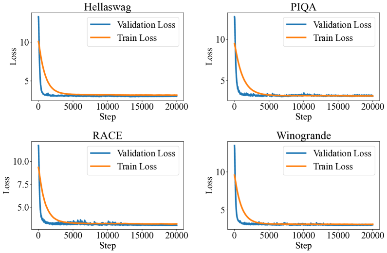
Figure 5: Training and validation loss during the flexible layer selection phase. The figure shows the training and validation loss over 20,000 steps for four different datasets (Hellaswag, PIQA, RACE, and Winogrande), where the batch size at each step is 1. The blue line shows the validation loss and the orange line shows the training loss. These plots visually compare how the performance of the models changes during the flexible layer selection phase, highlighting the convergence behavior.

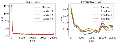
Figure 6: Comparison of train loss and evaluation loss in the Hellaswag dataset during the ablation study 5.3. This figure presents the train loss (left) and evaluation loss (right) over 20,000 steps for the Hellaswag dataset, where the batch size at each step is 1. The performance of the Flexora method is compared against three different random layer selection strategies (Random 1, Random 2, and Random 3). The train loss graph shows how the training performance of model evolves, while the evaluation loss graph highlights the generalization capability of model on the validation set. This detailed comparison provides insights into the effectiveness of Flexora relative to random selection methods in terms of both training and evaluation metrics.

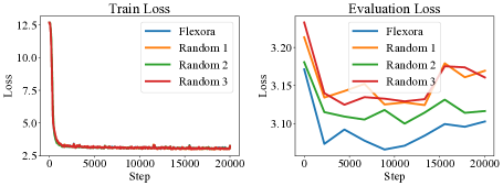
Figure 7: Comparison of train loss and evaluation loss in the PIQA dataset during the ablation study 5.3. This figure presents the train loss (left) and evaluation loss (right) over 20,000 steps for the PIQA dataset, where the batch size at each step is 1. The performance of the Flexora method is compared against three different random layer selection strategies (Random 1, Random 2, and Random 3). The train loss graph shows how the training performance of model evolves, while the evaluation loss graph highlights the generalization capability of model on the validation set. This detailed comparison provides insights into the effectiveness of Flexora relative to random selection methods in terms of both training and evaluation metrics.

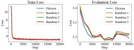
Figure 8: Comparison of train loss and evaluation loss in the RACE dataset during the ablation study 5.3. This figure presents the train loss (left) and evaluation loss (right) over 20,000 steps for the RACE dataset, where the batch size at each step is 1. The performance of the Flexora method is compared against three different random layer selection strategies (Random 1, Random 2, and Random 3). The train loss graph shows how the training performance of model evolves, while the evaluation loss graph highlights the generalization capability of model on the validation set. This detailed comparison provides insights into the effectiveness of Flexora relative to random selection methods in terms of both training and evaluation metrics.

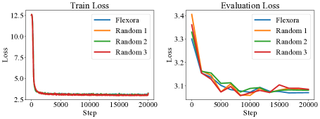
Figure 9: Comparison of train loss and evaluation loss in the Winogrande dataset during the ablation study 5.3. This figure presents the train loss (left) and evaluation loss (right) over 20,000 steps for the Winogrande dataset, where the batch size at each step is 1. The performance of the Flexora method is compared against three different random layer selection strategies (Random 1, Random 2, and Random 3). The train loss graph shows how the training performance of model evolves, while the evaluation loss graph highlights the generalization capability of model on the validation set. This detailed comparison provides insights into the effectiveness of Flexora relative to random selection methods in terms of both training and evaluation metrics.

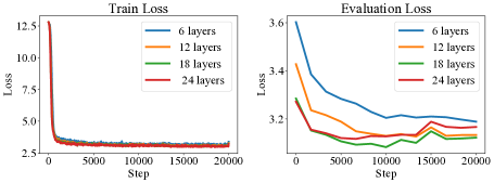
Figure 10: Training loss and evaluation loss during fine-tuning of different numbers of layers in the Flexora on the Hellaswag dataset. This figure presents the training loss (left) and evaluation loss (right) over 20,000 steps for the Hellaswag dataset. The performance is compared across four different configurations where the first 6, 12, 18, and 24 layers of the Flexora model are fine-tuned. The training loss graph shows that the model with 24 layers (red) achieves the lowest training loss, indicating it fits the training data very well. However, the evaluation loss graph reveals that the model with 18 layers (green) achieves the lowest evaluation loss, suggesting better generalization to unseen data. This discrepancy highlights the overfitting issue, where the model with 24 layers performs well on the training data but does not generalize as effectively as the model with 18 layers.

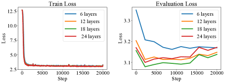
Figure 11: Training loss and evaluation loss during fine-tuning of different numbers of layers in the Flexora on the PIQA dataset. This figure presents the training loss (left) and evaluation loss (right) over 20,000 steps for the PIQA dataset. The performance is compared across four different configurations where the first 6, 12, 18, and 24 layers of the Flexora model are fine-tuned. The training loss graph shows that the model with 24 layers (red) achieves the lowest training loss, indicating it fits the training data very well. However, the evaluation loss graph reveals that the model with 18 layers (green) achieves the lowest evaluation loss, suggesting better generalization to unseen data. This discrepancy highlights the overfitting issue, where the model with 24 layers performs well on the training data but does not generalize as effectively as the model with 18 layers.

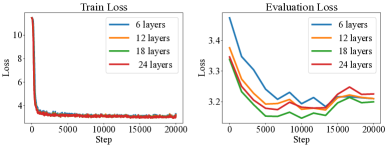
Figure 12: Training loss and evaluation loss during fine-tuning of different numbers of layers in the Flexora on the RACE dataset. This figure presents the training loss (left) and evaluation loss (right) over 20,000 steps for the RACE dataset. The performance is compared across four different configurations where the first 6, 12, 18, and 24 layers of the Flexora model are fine-tuned. The training loss graph shows that the model with 24 layers (red) achieves the lowest training loss, indicating it fits the training data very well. However, the evaluation loss graph reveals that the model with 18 layers (green) achieves the lowest evaluation loss, suggesting better generalization to unseen data. This discrepancy highlights the overfitting issue, where the model with 24 layers performs well on the training data but does not generalize as effectively as the model with 18 layers.

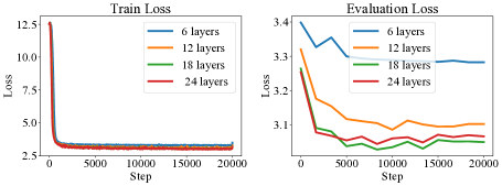
Figure 13: Training loss and evaluation loss during fine-tuning of different numbers of layers in the Flexora on the Winogrande dataset. This figure presents the training loss (left) and evaluation loss (right) over 20,000 steps for the Winogrande dataset. The performance is compared across four different configurations where the first 6, 12, 18, and 24 layers of the Flexora model are fine-tuned. The training loss graph shows that the model with 24 layers (red) achieves the lowest training loss, indicating it fits the training data very well. However, the evaluation loss graph reveals that the model with 18 layers (green) achieves the lowest evaluation loss, suggesting better generalization to unseen data. This discrepancy highlights the overfitting issue, where the model with 24 layers performs well on the training data but does not generalize as effectively as the model with 18 layers.

C.7 Special cases

This section details the performance of Flexora and LoRA across four distinct datasets. The results indicate that Flexora demonstrates superior comprehension and judgment on more challenging questions within the test dataset, compared to LoRA. In certain instances, Flexora successfully explains problems not previously encountered during training, showcasing its robust learning and generalization capabilities.

References

- Bao et al. (2021) Bao, F.; Wu, G.; Li, C.; Zhu, J.; and Zhang, B. 2021. Stability and Generalization of Bilevel Programming in Hyperparameter Optimization. arXiv:2106.04188.
- Bisk et al. (2019) Bisk, Y.; Zellers, R.; Bras, R. L.; Gao, J.; and Choi, Y. 2019. PIQA: Reasoning about Physical Commonsense in Natural Language. arXiv:1911.11641.
- Blair (1985) Blair, C. 1985. Problem complexity and method efficiency in optimization (as nemirovsky and db yudin). Siam Review, 27(2): 264.
- Chen et al. (2023) Chen, T.; Ding, T.; Yadav, B.; Zharkov, I.; and Liang, L. 2023. LoRAShear: Efficient Large Language Model Structured Pruning and Knowledge Recovery. arXiv:2310.18356.
- Contributors (2023) Contributors, O. 2023. OpenCompass: A Universal Evaluation Platform for Foundation Models. https://github.com/open-compass/opencompass.
- Franceschi et al. (2017) Franceschi, L.; Donini, M.; Frasconi, P.; and Pontil, M. 2017. Forward and Reverse Gradient-Based Hyperparameter Optimization. arXiv:1703.01785.
- Franceschi et al. (2018) Franceschi, L.; Frasconi, P.; Salzo, S.; Grazzi, R.; and Pontil, M. 2018. Bilevel Programming for Hyperparameter Optimization and Meta-Learning. arXiv:1806.04910.
- Fu et al. (2016) Fu, J.; Luo, H.; Feng, J.; Low, K. H.; and Chua, T.-S. 2016. DrMAD: Distilling Reverse-Mode Automatic Differentiation for Optimizing Hyperparameters of Deep Neural Networks. arXiv:1601.00917.
- GLM et al. (2024) GLM, T.; :; Zeng, A.; Xu, B.; Wang, B.; Zhang, C.; Yin, D.; Rojas, D.; Feng, G.; Zhao, H.; Lai, H.; Yu, H.; Wang, H.; Sun, J.; Zhang, J.; Cheng, J.; Gui, J.; Tang, J.; Zhang, J.; Li, J.; Zhao, L.; Wu, L.; Zhong, L.; Liu, M.; Huang, M.; Zhang, P.; Zheng, Q.; Lu, R.; Duan, S.; Zhang, S.; Cao, S.; Yang, S.; Tam, W. L.; Zhao, W.; Liu, X.; Xia, X.; Zhang, X.; Gu, X.; Lv, X.; Liu, X.; Liu, X.; Yang, X.; Song, X.; Zhang, X.; An, Y.; Xu, Y.; Niu, Y.; Yang, Y.; Li, Y.; Bai, Y.; Dong, Y.; Qi, Z.; Wang, Z.; Yang, Z.; Du, Z.; Hou, Z.; and Wang, Z. 2024. ChatGLM: A Family of Large Language Models from GLM-130B to GLM-4 All Tools. arXiv:2406.12793.
- Guo et al. (2020) Guo, L.-Z.; Zhang, Z.-Y.; Jiang, Y.; Li, Y.-F.; and Zhou, Z.-H. 2020. Safe deep semi-supervised learning for unseen-class unlabeled data. In International conference on machine learning, 3897–3906. PMLR.