Sparse Regression for Discovery of Constitutive Models from Oscillatory Shear Measurements
Abstract
We propose sparse regression as an alternative to neural networks for the discovery of parsimonious constitutive models (CMs) from oscillatory shear experiments. Symmetry and frame-invariance are strictly imposed by using tensor basis functions to isolate and describe unknown nonlinear terms in the CMs. We generate synthetic experimental data using the Giesekus and Phan-Thien Tanner CMs, and consider two different scenarios. In the complete information scenario, we assume that the shear stress, along with the first and second normal stress differences, is measured. This leads to a sparse linear regression problem that can be solved efficiently using regularization. In the partial information scenario, we assume that only shear stress data is available. This leads to a more challenging sparse nonlinear regression problem, for which we propose a greedy two-stage algorithm. In both scenarios, the proposed methods fit and interpolate the training data remarkably well. Predictions of the inferred CMs extrapolate satisfactorily beyond the range of training data for oscillatory shear. They also extrapolate reasonably well to flow conditions like startup of steady and uniaxial extension that are not used in the identification of CMs. We discuss ramifications for experimental design, potential algorithmic improvements, and implications of the non-uniqueness of CMs inferred from partial information.
I Introduction
Industrially important soft materials such as polymer melts and solutions, colloidal suspensions, gels, emulsions, foams, powders, etc., are non-Newtonian fluids.[1] The viscoelasticity of these complex fluids can be characterized by rheometry, in which the response of samples subjected to prescribed stress or deformation protocols is measured experimentally. Besides providing insights into material structure and behavior, such rheological measurements can guide the selection or construction of tensorial constitutive models (CMs), which mathematically describe the relationship between stress and deformation.[2, 3] These CMs, along with conservation equations for mass and momentum, can then be incorporated into computational fluid dynamics (CFD) software to predict complex flows in process equipment such as mixers, pipe bends, contractions, injection chambers, etc., under different operating conditions.[4, 5, 6] Thus, from an industrial standpoint, the development of reliable CMs for complex fluids can evade costly and time-consuming experimentation, and significantly accelerate the design and scale-up of new processes and products.
Traditionally, modelers use their experience and intuition to select a physically plausible CM. Once a CM is chosen, experimental data is used to calibrate its parameters. The advantage of this conventional workflow, especially for CMs based on microscopic physics, is that the parameters of the model are physically interpretable. The disadvantage is the problem of abundance or scarcity: Sometimes there are too many plausible CMs, while at other times there are none. Statistical tools for model selection are available to deal with the problem of abundance.[7] The problem of scarcity is more challenging. A potential recourse that has emerged in recent years is the use of rheological data to discover the underlying CM.[8, 9, 10, 11, 12]
Several data-driven or machine learning (ML) techniques have been proposed for the fusion of ML with CMs for rheological modeling, model identification, or calibration.[13, 14, 15, 16, 17, 18] A subset of these studies have focused on the discovery of CMs,[16, 11, 19, 12] which is the primary objective of this work. This enterprise is impeded by several obstacles:
-
(i)
Data is limited: Powerful ML methods thrive on digesting large quantities of information, and unearthing hidden patterns and correlations.[20] In contrast, rheological experiments are time-consuming, and the number of independent datasets is typically modest (even for well-characterized soft materials, ). This paucity of data makes it challenging to avoid overfitting powerful ML models, while still capturing the complexity of material behavior.
-
(ii)
Designing and training neural networks is an art: The vast majority of models that combine ML with nonlinear CMs use artificial neural networks (NNs) as universal function approximators.[13, 14, 15, 17, 11, 12] While the ubiquity and success of physics-inspired NNs clearly demonstrates their versatility and utility as black-box approximators, the design of suitable architectures and training protocols for optimizing parameters requires trial and error.[21] There are additional difficulties presented by (i) lack of convergence guarantees,[22] (ii) stiffness of differential equations,[23, 24] and (iii) sensitivity to network hyper-parameters.[25, 26, 27] The typical strategy leans on advances in automatic differentiation by throwing a versatile optimizer like stochastic gradient descent or its variants at the problem. Unlike traditional optimization of convex objective functions, the difficulty of convergence and absence of theoretical guarantees makes designing and training NNs a dark art.
-
(iii)
CMs that violate physical constraints cannot be used in CFD software: Typically, ML is used to select, calibrate, or discover a CM that fits rheological data by using a meta-heuristic or generalized nonlinear CM as a scaffold (we adopt this approach as well). Ideally, flow fields in rheometers used to collect rheological data are spatially uniform. CMs inferred from such data might not extrapolate well to non-uniform flow fields in process equipment. Unless special care is taken, CMs inferred using ML are not guaranteed to obey physical constraints like symmetry and frame-invariance. For example, in the popular physics-informed NNs (PINNs) framework, violation of conservation laws and physical constraints are penalized, but not strictly enforced.[28] Consequently, CMs are not guaranteed to obey physical constraints for all inputs. While such models may still be useful for interpolation between training datasets, even minor violations of physical constraints makes them potentially unusable in CFD software. A notable exception is the approach of Lennon et al. [11] that preserves strict symmetry and frame-invariance. Consequently, we adopt certain elements of their approach in this work.
-
(iv)
Inductive bias is desirable: A purely objective data-driven approach for discovering CMs seems attractive at first glance, until we confront it with the paucity of data in rheological characterization, and the inherent nonuniqueness of inferring a general CM based on only a few measurements. More colloquially, when data is scarce, it can fit many stories, some of which may be unnecessarily complicated or incorrect. Strict adherence to physical constraints and judicious inductive biases can reduce the search space of potential CMs. An inductive bias that animates this work is parsimony, the idea that simple models are preferable to complex models. Simple models that do not violate physical constraints avoid over-fitting, which increases the odds that they extrapolate satisfactorily to novel flow and process conditions.
I.1 Motivation and Layout
The primary goal of this work is to develop a protocol for the discovery of tensorial CMs from modest-sized rheological datasets that can then be embedded into CFD software. Thus, we strictly enforce physical constraints like symmetry and frame-invariance by relying on theoretical work on tensor basis functions (TBFs), which are introduced in section II.2.[11] This strongly limits the type of nonlinear terms that can appear in a CM, and shrinks the set of spurious CMs that nevertheless fit experimental data.
We also embrace the idea of parsimony in the hope of favoring simple interpretable CMs. This is accomplished by relying on sparse regression. A general introduction is provided in section II.3, which is specialized for the task of CM discovery in section III. A radical departure from previous work on ML for CMs is the complete avoidance of NNs. In addition to bypassing the sensitive and opaque choices in designing and training NNs, we aim to develop a more transparent framework with the expectation that different researchers confronted with the same experimental data will reliably arrive at comparable CMs. Furthermore, we would like the method to be fast and easy to implement. Thus, our objective is to learn the CM in on a desktop computer, using statistical techniques that do not require specialized hardware or ML training. Our overarching goal is to establish a pathway to democratize the discovery of CMs from experimental data.
To make progress on this ambitious task, we sharpen our focus by considering a narrower problem in this work. The key elements of our approach are:
-
•
Synthetic experimental data: Oscillatory shear (OS) rheology offer a convenient experimental route for systematically exploring the linear and nonlinear rheology of materials by imposing a sinusoidal strain or stress. Instead of using data on real materials, we intentionally use synthetic data using well-established CMs for polymers. The advantage of using synthetic data in a proof-of-concept study of this kind is that, unlike experimental data, the ‘true’ CM is known and can be compared against. This is helpful to characterize both the promise and inherent limitations of ML.
-
•
Framework for learning CM: Frame-invariance imposes strict limits on the structure of the time-derivatives in CMs (see Section II.1).[29] Here, we use an upper-convected derivative to model the evolution of stress,[2] and use data to learn the nonlinear terms of the CM. This provides a framework in which data can be incorporated by selectively learning only the unknown components of the CM. Furthermore, the unknown nonlinear term in the CM is expressed using TBFs to preserve physical constraints.
-
•
Spectral method for solving nonlinear CM in OS: We leverage a recently developed method called FLASH (Fast Large Amplitude Simulations using Harmonic balance) to obtain the periodic steady state (PSS) solution of arbitrary nonlinear differential CMs subjected to OS flow.[30] FLASH is a spectral method that is both fast and accurate, usually by orders of magnitude compared to the standard method of numerical integration via time-stepping methods.[31, 32] It solves for the PSS solution in Fourier space, which is a natural ansatz for steady state OS flow.
-
•
Sparse Regression: We express the task of ML as a sparse regression problem.[7] In special situations where all stress components are measured, this simplifies to sparse linear regression. Linearity puts the problem on a mathematically firm footing, where approximations and choices are automatically more transparent. Typically however, we end up with a more formidable sparse nonlinear regression problem.[33, 34] FLASH is the linchpin of our strategy in this scenario. Inspired by ideas of basis pursuit,[35, 36] we propose a simple greedy algorithm [37] in Section III.3.
Due to the large number of abbreviations and mathematical symbols used in this work, they are summarized for reference in the supplementary material Section LABEL:sec:nomenclature.
II Background
II.1 Constitutive Models and Oscillatory Shear
In constitutive modeling of viscoelastic liquids, we focus on the dependence of the extra stress tensor on applied deformation. It can be represented as a matrix, or using Einstein notation as , where , , and are unit vectors in Cartesian coordinates, and the combination can be thought of as a matrix whose only nonzero element is a one in the th row and th column.
Physics imposes important constraints on the form and evolution of . Due to the conservation of angular momentum, is symmetric and has only six independent components.[2] Due to the principle of material frame indifference, CMs are frame invariant.[29] This severely limits the possible forms for the time derivatives in CMs. Consequently, CMs are usually formulated in terms of the upper-convected, lower-convected, and corotational derivatives, or combinations thereof.[29] The upper-convected, lower-convected, and corotational derivatives of are given by,
| (1) | |||
| (2) | |||
| (3) |
respectively, where is the velocity field, is the velocity gradient tensor, and is the vorticity tensor. The upper-convected derivative defines the upper-convected Maxwell (UCM) model, which is a simple, linear but conceptually useful model given by[1]
| (4) |
where is the symmetric deformation gradient tensor. The UCM model has two material parameters: the relaxation time , and the shear modulus . For homogeneous flows such as those imposed in a rheometer, the stress field is uniform (), and the UCM model simplifies to
| (5) |
where denotes the time-derivative . In standard OS experiments, a sinusoidal strain (or stress) is applied, and the residual periodic stress (or strain) profile once the transient response has decayed is recorded. This residual solution is called the limit cycle or the PSS solution. In this work, we focus on OS strain experiments in which a sinusoidal strain of amplitude and frequency is imposed with and being the shear and shear gradient directions, respectively. Then, the velocity gradient tensor and the shear rate tensor , where the shear rate .
This simplifies the UCM model (Equation 5) in OS flow to a system of four ordinary differential equations
| (6) |
The other two components due to the geometry of the imposed deformation. In experiments, the periodic shear, , and normal stress differences and can be measured. If we assume a stress-free initial condition , then also drops out, and we only have to track three independent components of , namely , , and . Consequently, from a computational standpoint, the second normal stress difference throughout this work. Since the UCM model is linear, Equation 6 can be solved analytically to yield the PSS solution[38]
| (7) |
where the storage modulus , and the loss modulus . Although the UCM model is a conceptually useful model of viscoelasticity, its ability to describe real materials is severely limited due to linearity. To overcome this limitation, we can consider a generalized nonlinear differential CM based on the upper-convected derivative or the generalized UCM model as
| (8) |
where is a nonlinear but frame-invariant tensor function. Many popular physics-based CMs for polymer solutions and melts such as the Giesekus and the affine Phan-Thien Tanner (PTT) models fit this mold.
In the Giesekus model,[39] takes a quadratic form,
| (9) |
where the dimensionless parameter controls nonlinearity. The Giesekus model was originally developed to describe the nonlinear viscoelastic behavior of polymer solutions in both shear and extension. Subsequently, it has been applied to other systems such as worm-like micelles[40, 41, 42, 43, 44] and protein dispersions.[45, 46]
Similarly, for affine flow, the nonlinear term in the exponential PTT model is[47, 48]
| (10) |
where the extent of nonlinearity is controlled by a dimensionless parameter through an exponential function of the trace of ,
| (11) |
The PTT model for polymeric fluids is motivated by the Lodge-Yamamoto network theory,[49, 50] in which cross-links can be created and destroyed. The version described by Equation 10 applies for affine flows which assumes that there is no slip between the network and the continuous medium. The dimensionless parameter models the rate at which cross-links are destroyed in the network.[48] Typically, ranges from for dilute polymer solutions, to for polymer melts. Values approaching are considered unrealistic for describing real materials.[51] The exponential form of the nonlinearity qualitatively reproduces experimental data in strong flows,[3] and multi-mode versions of the model have been used to describe the behavior of real materials.[52, 53, 54]
The ordinary differential equations corresponding to the Giesekus and PTT models in OS are listed in supplementary material Section LABEL:sec:ode_models. Both the Giesekus and PTT models reduce to the UCM model when or are zero. However, unlike the UCM model, their OS response cannot be obtained analytically in general. The standard approach for obtaining PSS solutions of nonlinear CMs subjected to large-amplitude oscillatory shear (LAOS) is numerical integration using a suitable time-stepping method like Runge-Kutta.[55] However, this approach can be computationally expensive because of the need for implicit methods to address numerical instability at large values of and , and to mitigate long transients.
Recently, we developed a fast and accurate spectral method called FLASH to compute the PSS solution of any nonlinear differential CM subjected to OS strain.[30] It is based on the technique of harmonic balance,[56, 32, 31] which uses Fourier transforms to convert a system of nonlinear ordinary differential equations into a system of nonlinear algebraic equations in the Fourier coefficients. FLASH couples harmonic balance with a numerical scheme called alternating-frequency-time, which transforms the nonlinear terms in the CM to the frequency space and back during each iteration of the solver. The mathematical ideas behind this approach are presented in Section LABEL:sec:hb_flash of the supplementary material.
FLASH offers a convenient interface to identify the OS response of arbitrary differential CMs. The methodology is not restricted to CMs based on the generalized UCM model (Equation 8), although that is the form used here. As input, FLASH takes in a fully parameterized differential CM, operating conditions ( and ), and a parameter which specifies the ansatz. FLASH exploits the even and odd symmetries of the normal and shear stresses, respectively, and resolves them up to the harmonic. Based on previous experience,[32, 30] we set throughout this work for simplicity, although this assumption can be easily relaxed if required. FLASH shifts the burden of setting up and solving the relevant set of harmonic balance equations from the modeler to the computer. The most attractive attributes of FLASH in this work are its accuracy and speed. In these benchmarks, FLASH typically outperforms numerical integration by 1–3 orders of magnitude.[32, 31, 30]
II.2 Nonlinear Constitutive Models using Tensor Basis Functions
Consider symmetric, frame-invariant 33 matrices , , and , where is an arbitrary analytic function of and . Using the Cayley-Hamilton theorem (see appendix A), can be represented as a polynomial of degree two in and ,[57, 58, 59, 60]
| (12) |
where tensor dot products and are equivalent to matrix multiplications. The coefficients are polynomials in the 10 invariants of and given by the traces of the following 10 matrices: , and . This set of 10 matrices contains all possible matrix products with .
Equation 12 provides a finite set of basis functions with which any symmetric, frame-invariant, smooth 33 matrix function can be represented. Lennon et al.[11] recognized the importance of this result for inferring nonlinear CMs from experimental data. They used the generalized UCM model (Equation 8) as a scaffold and represented the unknown nonlinear term as a linear combination of polynomials in and according to Equation 12, leading to
| (13) |
where is the set of TBFs, is the set of invariants, and is the set of scalar coefficient functions (SCFs), with . The TBFs and invariants are listed in Table 1. Note that only 9 invariants () are listed instead of the 10 anticipated,[57, 59] because tr() = 0 for incompressible fluids, eliminating one of the invariants from the original set.
Lennon et al. proposed a framework called rheological universal differential equations (RUDE).[11] Universal differential equations represent a marriage of ML and differential equations, and embed universal functional approximators such as NNs within differential equations. By representing the nonlinear term using Equation 13, the goal of inferring a nonlinear CM boils down to learning the SCFs through by fitting experimental data. The RUDE framework accomplished this task by modeling using a deep NN. Several advantages of this approach were observed. It worked well with limited experimental data and different deformation protocols. It also extrapolated to processing flow conditions surprisingly well.[11]
| TBFs | invariants |
|---|---|
In this work, we restrict ourselves to OS measurements. As mentioned previously, has only two nonzero elements, and has only three unique nonzero elements. This further simplifies the expressions for the TBFs and invariants (see Appendix B): in particular, there are only = 5 independent invariants, . Thus, we can attempt to learn the SCFs from OS data using this abridged set of invariants.
II.3 Sparse Regression
In this work, we infer (more precisely, ) using sparse regression, instead of NNs, for the following reasons:
-
(i)
a sparse regression model for with only a few nonzero algebraic terms () is potentially easier to interpret than a NN with parameters;
-
(ii)
the fact that SCFs are polynomials can be naturally embedded into the regression process;
-
(iii)
under special conditions in which all the nonzero stress components are measured, the optimization problem reduces to sparse linear regression (SLR), which permits a fast, robust, and transparent solution (Section III.2);
-
(iv)
under typical conditions in which only the shear stress is measured, the optimization problem leads to a non-convex sparse recovery problem, which can be approached with greedy algorithms (Section III.3).
We label the scenario in which all the nonzero stress components are measured as the complete information or CI scenario. In experiments, this includes the shear stress , the first normal stress difference , and the second normal stress difference . This represents an idealized case, since most OS experiments do not measure due to experimental difficulties and only occasionally report . Therefore, for the more realistic scenario of partial information (PI) we assume that only the shear stress () is available. Specific methods for CM discovery in these scenarios are described in Section III. In the following, we provide a general introduction to SLR and sparse nonlinear regression (SNLR).
II.3.1 Sparse Linear Regression
Consider the linear least-squares (LS) solution of an over-determined linear system , where is a vector of observations, and is an matrix of predictors with . The goal of linear LS regression is to find the combination of the columns of that most closely resembles , i.e., . Since the system is over-determined, an LS solution attempts to solve the minimization problem
| (14) |
where represents the -norm of vector . The LS solution can be obtained by solving the normal equations, or using QR decomposition.[55] Typically, most elements of the resulting are nonzero, suggesting that all the columns of are required to predict . The preference for parsimony can expressed by requiring to be sparse, with most entries equal to zero.
A popular sparsity-promoting convex optimization technique called LASSO (least absolute shrinkage and selection operator) [61] or basis pursuit [62] combines regularization and variable selection.[63, 64, 7] It appends an regularization term to the LS objective function to penalize overfitting:
| (15) |
The magnitude of the parameter simultaneously controls the strength of variable selection and regularization. As , . As , the regularization term dominates the objective function, and leads to the trivial solution . The optimal value of , which lies somewhere between these extremes, seeks a trade-off between the need to describe the experimental observations well, the ability to pose a well-conditioned problem, and to produce a sparse solution. Often, is selected using cross-validation.[7, 64]
LASSO is a versatile regression technique that works for both over-determined () and under-determined () linear systems. In the latter case, it enables us to take a kitchen-sink approach by embedding all potential predictive information into the columns of , relying on LASSO to select the truly relevant set of predictors.[64] This attractive property of LASSO to identify sparse solutions is sometimes called feature selection. Since LASSO combines variable selection and shrinkage, the nonzero elements of are biased toward zero. This bias can be reduced by using LASSO to identify the nonzero components, and refitting an unrestricted linear model or using LASSO again, only on the selected components.[7] Many efficient algorithms for finding such as least angle regression,[65] coordinate-wise optimization,[66] and basis pursuit[62] have been proposed. The cost per iteration is on the same order as linear LS regression, i.e., .[65]
II.3.2 Sparse Nonlinear Regression
Consider , where is a noisy response or output variable, is a covariate or input variable, and is a vector that parameterizes the nonlinear model . Given a set of observations , corresponding to inputs , the sparse nonlinear recovery problem may be posed as minimization of an LS loss function,
| (16) |
where is a positive integer that controls the number of nonzero elements in via the 0-norm . Even if the regularization penalty in Equation 16 is replaced by an regularization term (similar to Equation 15 in LASSO regression), we have to contend with a non-convex optimization problem because is nonlinear.[34] Compared to sparse linear regression, this is a much harder problem. Nevertheless, substantial theoretical progress has been made in establishing sufficient and necessary conditions for the recovery of sparse or structured signals from relatively few nonlinear observations.[67, 33]
Different algorithms inspired by sparse linear regression for compressed sensing applications such as iterative hard thresholding, and basis pursuit have been adapted for sparse nonlinear regression.[68, 69] Each iteration of a typical thresholding algorithm alternates between a regular gradient descent step followed by a hard or soft thresholding step, in which all but the largest elements of by magnitude are set or pushed toward zero.[33, 67, 34, 70] Since the sparse nonlinear recovery problem is NP-hard,[71] an alternative approach inspired by basis or matching pursuit,[35, 36] adopts a greedy approach in which locally optimal choices are proposed at each iteration to obtain an approximate solution. In this class of methods,[69, 33, 72] promising features of are iteratively marked for inclusion depending on how effective they are in reducing the loss function locally.
III Methods
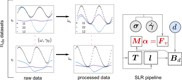
In this work, we first generate synthetic data with different combinations of strain amplitude and frequency (, ) using the Giesekus and PTT models. We set the linear viscoelastic parameters and equal to one, so that they set the units of stress and time, respectively. We set the nonlinear parameters for the Giesekus model and for the PTT model. We generate synthetic datasets from three different frequencies that span the relaxation time (), and four different strain amplitudes , focusing on the medium and large amplitude regimes to elicit a vigorous nonlinear response. We use FLASH with to compute the PSS solution up to the 17th harmonic. For the range of parameters and operating conditions explored in this work, the magnitude of the intensity of the 17th harmonic relative to the 1st harmonic is less than . For each choice of , , the periodic solution (, , and ) is obtained over one cycle on a uniform temporal grid with points.
Before we present specific methods to infer the SCFs for the CI and PI scenarios, we discuss the approach to specify a set or dictionary of potential features with which to capture the mathematical dependence of the SCFs () on the invariants (). This step is required for both linear and nonlinear sparse regressions.
III.1 Dictionary of Polynomial Features
| PFs | |||
|---|---|---|---|
| 0 | 1 | 9 | |
| 1 | 6 | 54 | |
| 2 | 21 | 189 | |
| 3 | 56 | 504 | |
| 4 | 126 | 1134 |
As mentioned in section II.2, for OS flow the SCFs are polynomials in independent invariants, . Mathematically, we approximate for by restricting the representation of the polynomial features up to a specified degree. Let be the degree of polynomial approximation for , and let denote the set of all unique polynomial combinations of the invariants with degree less than or equal to . Let us make this notion more concrete by considering a toy example with invariants, and . If , then the set of polynomial features (PFs) is . The elements of constitute PFs, . As and increase, also increases. In general, the number of PFs can be expressed using the binomial coefficient as
| (17) |
In the toy example, and . Thus, there are PFs in . We approximate the th SCF as
| (18) |
The coefficients () are the unknowns. In the toy example, this implies,
| (19) |
Discovery of the CM from experimental data is thus reduced to determining the coefficients.
For OS experiments, 6, 21, or 56 and 54, 189, and 504, for 1, 2, or 3, respectively (see Table 2). Although this increase with may seem explosive, a relatively small often suffices to describe highly nonlinear behavior because most of the invariants and TBFs are themselves nonlinear. As we shall see shortly, is sufficient to describe the Giesekus model. Even the exponential PTT model can be approximated by , under suitable conditions.
Thus, the number of unknown coefficients is modest, especially when compared to the number of parameters in deep NNs. In sparse regression, most of these coefficients turn out to be zero. In what follows, we use the symbol to denote the vector in which these coefficients are stacked. Depending on the context, these elements are indexed as where and , or simply as where . Computationally, this is equivalent to reshaping into a matrix or a vector.
III.2 Inference under Complete Information
Let begin with the simpler case of CI in which raw data consists of the = 3 nonzero stress components, , , and reported at the different settings of frequency and strain amplitude (see Figure 1). In an actual experiment, this implies that, in addition to shear stress, both and are also measured. For each dataset in this scenario, we report the PSS profiles obtained via FLASH at equispaced points over a period of oscillation, . Thus, all the components of are effectively known, since components that are not directly specified can either be inferred from symmetry () or set equal to zero (all other components).
Since and are known, we can substitute them into the generalized UCM model (Equation 8) to isolate and evaluate the nonlinear term for each dataset ,
| (20) |
is symmetric and frame-invariant like , and for OS flow it has = 3 independent components – , , and – that are also periodic functions. The time-derivative required to obtain in Equation 20 is computed by first transforming into Fourier space to obtain , and truncating beyond the th harmonic. We represent such truncated Fourier coefficients using a “hat”. Next, we take the inverse Fourier transform of to obtain . Both these steps are implemented efficiently using fast Fourier transforms (FFT).
The TBFs and invariants are also periodic and can also be evaluated using and using equations described in Appendix B. Thus, , , and are periodic functions that can be provided for each data set using and . The nonlinear term can then be approximated using Equations 13 and 18 as
| (21) |
When the polynomial approximation degree is assumed, the PFs are specified. Equation 21 is a linear regression problem in the unknown coefficients , since all the other quantities can be evaluated using and .
Let us now mathematically define the loss function that we seek to minimize. The loss function can be expressed as the sum of squared residuals (SSR) over all the observations:
| (22) |
It involves summation over five indices: over the SCFs, over the PFs, over the discrete time points, and over the different datasets . In Equation 22, the squared norm of a 3 3 symmetric matrix with three independent nonzero elements , and is defined as . The quadratic dependence of on leads to the linear LS problem , where is an dimensional vector of unknown coefficients, is a vector with elements of “observations” , and is a matrix whose elements are obtained from the invariants, PFs, and TBFs.
LASSO can then be used to seek a sparse solution,
| (23) |
where an regularization term is appended to the loss function,
| (24) |
We find the optimal value of by 5-fold cross-validation using the built-in function LassoCV from the linear_model module of the Python machine learning library scikit-learn version 1.11.[73] This implementation uses coordinate descent to fit the unknown coefficients and a duality gap calculation to control convergence.[66, 74]
LASSO automatically identifies the most important PFs and sets for other features.[63] Thus, even if we specify a large number of redundant PFs, LASSO isolates the handful of features that primarily explain the observations. This helps to investigate the source of nonlinearity when the underlying CM is unknown. The algorithm used for the CI scenario is summarized as Algorithm 1. As input, it takes in experimental data which includes the operating conditions and the components of for each dataset. The degree of polynomial approximation is also specified as input. The raw experimental data are processed to obtain the nonlinear term which eventually forms the right-hand side of the linear system. The matrix requires TBFs and invariants that are reconstructed from experimental data, and the set of polynomial features , which are constructed using the invariants and . The optimal value of the regularization parameter is found using 5-fold cross-validation, and the sparse solution is obtained by minimizing in Equation 24.
III.3 Inference under Partial Information
Once a degree of polynomial approximation is selected, the resulting approximation to the nonlinear term (Equation 21) can be substituted into the generalized UCM model (Equation 8) to define the TBF-CM as
| (25) |
The TBF-CM is a special case of the generalized UCM model like the Giesekus and PTT models. The nonlinear terms of the Giesekus and PTT models are parameterized by a single coefficient ( and , respectively). On the other, the nonlinear term of the TBF-CM is parameterized by a set of coefficients that are likewise independent of and . In other words, is a material property that is independent of the flow field. If is specified, then the TBF-CM is a fully parameterized nonlinear differential CM. This implies that we can use FLASH to solve for the PSS solution of the TBF-CM given and . FLASH relying on harmonic balance, internally transforms the resulting system of nonlinear differential equations into Fourier space and returns the Fourier coefficients of the PSS solution truncated beyond the th harmonic.
While it is easy to use inverse FFT to compute the time-domain representation, it is preferable to work in Fourier space for a few reasons. First, we can take Fourier transforms of any experimental data in the time domain to obtain . A byproduct of this operation is that the high-frequency noise in is filtered. Second, the Fourier space provides a natural basis for describing periodic signals. A byproduct of this choice is that it allows us to compress data by exploiting the correlation between successive time-domain snapshots of .
In summary, given coefficients and the deformation gradient tensor for OS flow, we can efficiently find the PSS by solving the TBF-CM using FLASH. Discovering a CM from experimental data corresponds to the inverse problem, i.e., inferring a sparse that yields .
III.3.1 Experimental Data and Loss Function
Similarly to the CI scenario, we generate synthetic experimental datasets by using FLASH to solve the PTT model for (or ) in OS flow using with and . However, we ignore some of the components of the stress tensor in the PI scenario. We pretend that we only have access to shear stress and discard information regarding normal stresses and .
Let denote the Fourier coefficients of the experimental PSS shear stress profile corresponding to the th dataset () with the deformation gradient tensor defined by the imposed strain frequency and amplitude. Only the subset is used for inference. Once we choose a degree of polynomial approximation , the size of the coefficient vector is determined. Let denote the Fourier coefficients of the shear stress profile predicted by the TBF-CM with coefficients and deformation gradient tensor .
We can evaluate how well a particular guess for matches experimental measurements by defining a LS loss function in Fourier space that sums over all the datasets,
| (26) |
Recall that both, and , are vectors of the same size. It is possible to find an optimal by attempting to minimize using nonlinear LS. However, we do not pursue this direct approach because it does not impose sparsity on , and is computationally challenging. Unlike the CI scenario, minimization of requires us to solve for under each of the operating conditions during each iteration. If the cost per iteration were proportional to , it would not pose a major challenge for datasets of modest size, say due to the speed of FLASH. However, if we use a minimizer that numerically computes the gradient to accelerate convergence,[55] the computational cost rises sharply from to per iteration, which can become exorbitant (see Section V.2 for a potential solution).
III.3.2 Sparse Nonlinear Regression
Recall that the SNLR problem, fashioned after Equation 16, may be formulated as
| (27) |
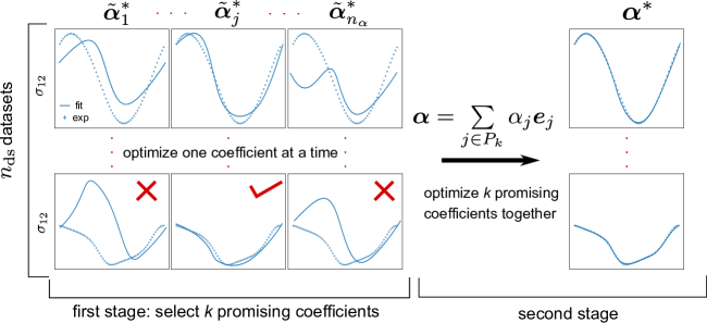
We propose a simple greedy algorithm, schematically illustrated in Figure 2, to determine a sparse . It is inspired by basis pursuit methods which attempt to identify and retain only the most promising features. We divide the task of inferring into two parts. In the first stage, we explore the potential of each individual element , where , to capture the data. In the second stage, we perform sparse nonlinear LS regression using only the most promising indices/coefficients.
In the following, let denote a unit vector of size with a single nonzero element at the location . In other words, the th element of is one, while the rest are equal to zero (similar to ‘one hot encoding’ in ML). Then, denotes a coefficient vector with a single nonzero element. In the first stage, we can perform a nonlinear LS minimization of and determine the optimal value , for each . This is an independent 1D optimization for each coefficient that can be readily parallelized. For each 1D optimization, the cost per iteration is making the total cost times the cost of each 1D optimization. Note that this is significantly better than per iteration, since the cost per iteration does not depend on , and the overall cost can be shared between multiple processors.
Promising coefficients are operationally defined as coefficients that result in small values of the loss function . We sort for in ascending order and consider only the top coefficients. Let denote the list of indices of these top most promising coefficients. The elements of are integers that mark the locations of these coefficients. The goal of the first stage is to furnish .
In the second stage, we perform a nonlinear LS regression to minimize , where sparsity is imposed on by construction. That is, we set
| (28) |
where the summation runs over the list of elements in . Thus, has only nonzero elements corresponding to the most promising indices. The cost per iteration at this stage is , where .
We solve all nonlinear minimization problems using the default trust-region reflective algorithm as implemented in the scipy.optimize library.[75] For unbounded optimization, used in this work, this implementation is quite robust and similar to the implementation in MINPACK.[76, 77] The derivatives are computed numerically using a 2-point scheme. Algorithm 2 summarizes the steps sketched in Figure 2. Input data consists of the Fourier coefficients of the shear stress and operating conditions for each dataset. The degree of polynomial approximation and number of nonzero coefficients are also provided as input. Note that it is possible to determine a judicious value for by examining the outcome of the first stage, in which the ability of each coefficient to describe experimental data is explored. The second stage performs a regular nonlinear LS calculation by allowing only the most promising coefficients to be nonzero.
IV Results
As mentioned previously, we generated synthetic datasets for the Giesekus () and PTT () models and computed the PSS solution using FLASH with and . We describe the results for the CI scenario, followed by the results for the PI scenario.
 |
 |
| (a) | (b) |
IV.1 Complete Information
IV.1.1 Giesekus Model
In the CI scenario, all components of the stress tensor are known, which allows us to evaluate the nonlinear term . We added a relative Gaussian noise of 20% to the nonlinear signal () for the Giesekus model, as illustrated in Figure 3 for two of the datasets. We perturbed instead of because filtering noise from raw experimental data using standard Fourier analysis is a fairly common practice. We set the degree of polynomial approximation , which implies that the number of PFs is . The set of features includes one constant (1), five linear terms (, and 15 unique quadratic () terms. The number of unknowns (size of ) is .
To contextualize the results of SLR, it is helpful to first consider the representation of the Giesekus model in terms of the TBFs. The form of the nonlinearity in the Giesekus model (Equation 9) coincides with one of the TBFs namely (see Table 1). Thus, , which implies that is a constant, while all other SCFs are zero, i.e., for .
 |
 |
| (A) Giesekus | (B) PTT |
As expected, using Algorithm 1, we find that only one of these 189 coefficients (namely ) is nonzero. The regressed value of shows that this technique identifies the true CM, at least for this simple example. The coefficient of correlation . This example serves as a validation test of the proposed method. Furthermore, this calculation is fast, since the problem is linear. It took about 0.5 sec on an old commodity desktop computer (Intel i7-6700 3.4 GHz CPU). Recall that the CI scenario, unlike the PI scenario, does not require the computation of the PSS solution using FLASH or numerical integration to find the optimal set of coefficients.
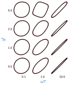
An elastic Lissajous-Bowditch curve is a parametric plot of stress versus strain. Figure 4 depicts a Pipkin diagram which is a table of normalized elastic Lissajous-Bowditch curves for the = 12 datasets. Here, the shear stress ( component of ), normalized by its maximum value, is plotted against the normalized strain . Symbols denote synthetic data (20% relative noise is only added to ), while lines show the TBF-CM which is nearly identical to the true CM in this case.
In a typical use case, is not noisy since the measured signal () can be filtered using Fourier analysis. If we use a noiseless as input, then the true CM is discovered using Algorithm 1. The true CM with a single nonzero component is discovered even when we increase corresponding to , or corresponding to . As expected, the computational time increases with as the size of the regression problem increases. The CPU time increases from 0.5 s for to 1 s for and 3 s for .
Thus, we validated Algorithm 1 for the Giesekus model and found that it is able to discover the true CM in the CI scenario using only the PSS stress profile for datasets of modest size (). Indeed, for the Giesekus model, which has a particularly simple representation in terms of the TBFs, we found that synthetic data generated at a single value of (that is, = 3, due to three frequencies) were sufficient to discover the true CM. The value of must be large enough to trigger a detectable nonlinear response, otherwise does not contain enough information. SLR is remarkably fast and fairly robust (it is not particularly sensitive to perturbations 20% in ), because the optimization problem is well posed.
While this example provides a glimpse of the promise of this method, caution is warranted. First, the CI scenario is not representative of practical problems. Second, the Giesekus model plays into the strengths of the method because of its simple structure. Therefore, we consider the PTT model under the CI scenario next, before moving to the harder problem of PI.
IV.1.2 PTT Model
As before, we generated synthetic datasets using the exponential PTT model with parameter . We set and obtained the nonlinear term . Of the possible coefficients, Algorithm 1 identified only two nonzero components of . Both these coefficients, namely and , correspond to the SCF . All other SCFs were zero. Therefore, according to SLR, the nonlinear term corresponding to data generated from the PTT model is,
| (29) |
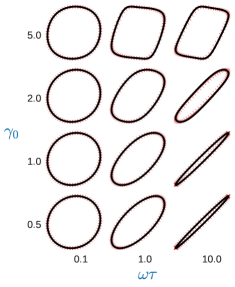
where and . The Pipkin diagram comparing the experimental elastic Lissajous-Bowditch curves with the inferred CM is shown in Figure 4B.
Unlike the Giesekus model, the exponential PTT model cannot be easily decomposed in terms of TBFs, except in special situations. In the limit of small and , the nonlinear term can be approximated as
| (30) |
Terms of order and higher are neglected in the Taylor series expansion in Equation 30. Thus, the only nonzero SCF is , which only depends on . Comparison of in eqns 29 and 30 indicates that the prefactor to (0.306) is comparable with . However, the second term in Equation 29, , is different from the , expected from Equation 30. Interestingly, if we use 0.1 instead of 0.3 to generate the synthetic datasets, SLR identifies a single nonzero coefficient and , which is similar to Equation 30.
As in the Giesekus model, increasing the polynomial approximation to effectively discovers the same TBF-CM, but takes 2.5 s instead of 0.5 s for . Unlike the Giesekus model, a single LAOS dataset is no longer sufficient to infer the CM. With some experimentation, we found that the CM with a nonlinear term given by Equation 29 is usually discovered, even if we use only three values of instead of four, e.g. . That is, appears to be sufficient for the PTT model. The key generalizable lesson from these examples for experimental design is to collect sufficient data in the LAOS regime (roughly, ).
IV.2 Partial Information
In this section, we demonstrate the application of the SNLR algorithm (Algorithm 2) to synthetic data obtained using the PTT model with under different operating conditions. However, unlike the CI scenario, we only use shear stress data for inference. We focus on the PTT model because it produces more interesting results and offers generalizable lessons that are relevant for CM discovery. Results for the Giesekus model are relegated to supplementary material Section LABEL:sec:Giesekus_PI.
As before, we set , which implies . In the first stage, we scan through for by performing independent 1D nonlinear minimizations to obtain optimal values and the corresponding loss functions . The average cost of each of these minimizations was 25.2 16.4 s, or approximately half a minute. On a computer with a single core, the first stage can be completed in about an hour and a half. On a workstation with 16 cores, this cost reduces to a little under 6 minutes, due to the ease of parallelization.
The computational cost is proportional , which implies that the cost of the first stage increases rapidly with . If we increase the degree of approximation from to , the total computational cost increases 6x, assuming that the average cost per minimization remains unchanged. On a workstation with 16 cores, the total runtime for the first stage increases to about 40 minutes.
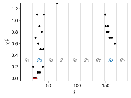
The corresponding to the most promising coefficients is shown in Figure 5. The first stage correctly identifies the importance of for the PTT model. The top most promising coefficients form a distinct cluster with , and are indicated by red stars. In order of increasing , these coefficients, namely , , , and , correspond to PFs , , , and , respectively.
For the second stage of Algorithm 2, in addition to , we also entertained the idea of retaining only the top coefficients to explore the possibility of multiple solutions, and sensitivity to the choice of . Thus, we considered two different sets of nonzero coefficients, , and . That is, in the set , we picked the top most promising coefficients, while in the set , we selected only the top most promising coefficients. We then performed a nonlinear regression that allowed only these coefficients to vary and ended up with two distinct TBF-CMs. They correspond to,
| (31) |
Hereafter, we label these two TBF-CMs as TBF-CM-k4 and TBF-CM-k3. The computational cost of the second stage of the SNLR algorithm is relatively small compared to that of the first stage. For instance, TBF-CM-k4 required 8 iterations which took 40 sec, while TBF-CM-k3 required only 6 iterations, which took 25 s. The final values of the loss function after optimization were and for TBF-CM-k4 and TBF-CM-k3, respectively.
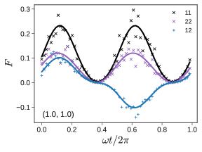
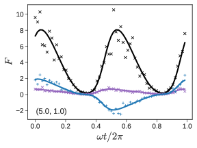
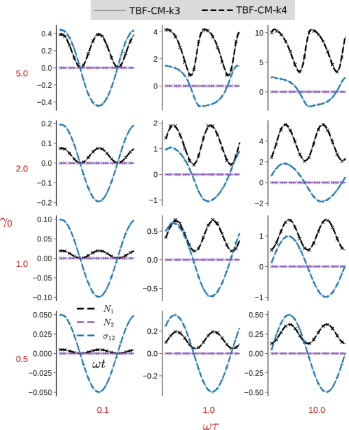
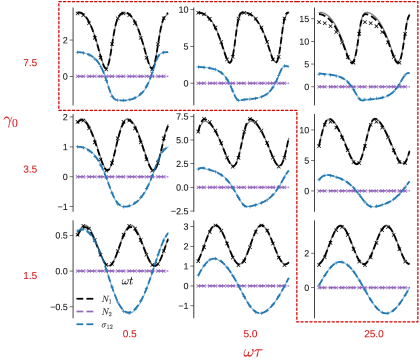
The fits of these two TBF-CMs and the experimental data are shown in Figure 6, where the dashed and thin lines represent TBF-CM-k4 and TBF-CM-k3, respectively. The symbols show the output of the PTT model. Although , and are all shown, it is important to remember that only the shear stress component is used in both stages of Algorithm 2. Visually, the agreement of both TBF-CMs with the data is excellent across the board. Experiments with and , produced fits that were qualitatively similar, but visually inferior.
This success is noteworthy for at least two reasons. First, although only shear stress data is used for inference in the PI scenario, the agreement of the predicted and with the PTT model is remarkable. Second, TBF-CM-k4 and TBF-CM-k3 look quite different from the TBF-CM inferred in the CI scenario, namely , which we subsequently label TBF-CM-CI, and the Taylor expansion of the PTT model in the limit of small and , namely . We examine the origin and implication of these two observations in succession.
Although the agreement of and predicted by the TBF-CMs with the PTT model is a fortunate accident that is unlikely to generalize to real materials, it is aided by the strict enforcement of physical constraints, and bias for parsimony. In particular, we observe that both TBF-CM-k4 and TBF-CM-k3 correctly predict . Retrospectively, this can be interpreted as a direct consequence of . When the nonlinear term is proportional to , remains unperturbed, if the initial condition , regardless of the functional form of .
The extraordinary agreement of and predicted by the TBF-CMs and the unseen synthetic data can be traced to the common origin of the nonlinear term for , , and . In particular, the components of for the PTT model in Equation 10 corresponding to these terms take the form , , and . Thus, if a good approximation for is obtained from the shear stress data, we expect it to also be a reasonable approximation for and .
What about the uniqueness of the inferred TBF-CM? TBF-CM-k4 and TBF-CM-k3 are products of Algorithm 2, which is a crude method for SNLR. In the PI scenario, we expect different CMs to result from different algorithms and parameter choices. The fact that at least three different CMs (TBF-CM-k4, TBF-CM-k3, and TBF-CM-CI) successfully describe shear stress data from a simple model like the PTT model underscores the inherent nonuniqueness of any CM discovered from limited data. Somewhat paradoxically, this nonuniqueness highlights the importance of frame invariance and inductive biases in navigating the space of potential CMs.
IV.2.1 Generalizability of TBF-CMs
The TBF-CMs inferred using the proposed algorithms fit experimental or training datasets remarkably well. However, what we usually care about for CFD applications is the ability of the learned model to generalize beyond the data used to train it. In this work, we know the true CMs (Giesekus or PTT). Therefore, we can compare the predictions of the inferred TBF-CMs with the true CMs beyond the training data.
We assess the generalizability of TBF-CM-k4 and TBF-CM-k3 by performing two different types of tests. In the first type, we consider the predictions of the TBF-CMs in OS flow, where the operating conditions are different from those used in the training datasets. Some of the in these tests lie within the region circumscribed by the experimental data. We label these predictions as interpolations. In other cases, lie outside the range of the training data. We label these predictions of the inferred TBF-CMs as extrapolations.
In the second type of experiment, we test the ability of the inferred CMs to generalize beyond the OS flow. These are much tougher benchmarks. In particular, we consider the predictions of the TBF-CMs to the startup of steady shear flow in which a constant shear rate is applied to an initially relaxed material (). Finally, we transition from shear flows to uniaxial extensional flows in which we consider the evolution of the normal stresses when a steady elongational strain rate is applied.[2]
In Figure 7, we show the results of the first type of test (OS shear). Recall from Figure 6, that the range of training data span , and . The four tests in the lower left corner of Figure 7 with equal to , , , and lie within the convex hull of the training data. Thus, they represent interpolations. The other five datasets in the figure marked off by the red dashed line lie outside the range of training data and hence represent extrapolations.
Visually, we find that the predictions of TBF-CM-k4 and TBF-CM-k3 are comparable and largely agree with the PTT model. On closer inspection, we find that TBF-CM-k4 is slightly superior, especially in describing . As increases well beyond the range of the training data (top right corner of Figure 7), predictions of start to become less satisfactory. From numerical experiments, we find that both the TBF-CMs extrapolate satisfactorily beyond the training data (see supplementary material Section LABEL:sec:extrap_pi_os). At large and strain amplitude (), it is advisable to resolve a greater number of harmonics (use larger ), and/or use more intermediate steps to aid the convergence of FLASH. Regardless, TBF-CMs using Algorithm 2 appear to generalize well for the PTT model in OS flow.
Next, we consider the second, more stringent, type of test in which we probe the behavior of TBF-CM-k4 and TBF-CM-k3 when a constant deformation rate is applied under shear and uniaxial extension. In steady shear flow, the velocity gradient tensor and the deformation gradient tensor , are the same as for OS flow. The only difference is that the shear rate is constant rather than sinusoidal. In uniaxial extension, the velocity gradient tensor is diagonal , where is the steady extensional strain rate. This implies that the shear rate tensor and the stress tensor have three nonzero components along the diagonal. TBFs and invariants specialized for uniaxial extension are presented in the supplementary material (Section LABEL:sec:TBF_unaxial).
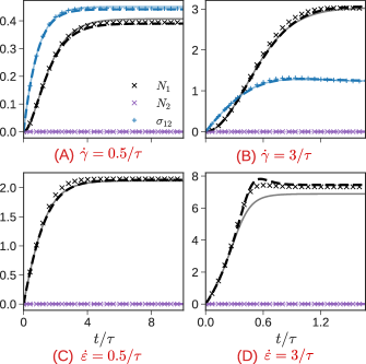
We solve the initial value problem using an implicit Runge-Kutta method belonging to the Radau IIA family implemented in the Python package scipy.[78, 79] It is a fifth-order method with local error controlled via a third-order accurate embedded formula. We assume that stress tensor components are initially zero, i.e., . In steady shear, we compute the evolution of the shear and normal stress components, whereas in steady uniaxial extension, we compute the evolution of only the normal stress components, since . For the PTT model, , as mentioned earlier.
We consider two different deformation rates ( and ) of 0.5/ and 3/. Comparisons of the PTT model and the TBF-CMs are shown in Figure 8. For the startup of steady shear, both TBF-CMs appear to work reasonably well. TBF-CM-k4 appears to be slightly more accurate in predicting shear stress. For , both models appear to capture the initial growth, but slightly under- or over-estimate the steady-state value.
A similar trend is also observed in the uniaxial extension. TBF-CM-k4 describes better, especially at , where TBF-CM-k3 under-estimates the steady state. It captures the mild overshoot in at large semi-quantitatively, but exaggerates the bump. Nevertheless, these out-of-sample tests show that the TBF-CMs inferred from PI using only data in OS experiments, generalize surprisingly well to startup shear and extension. Therefore, we speculate that they will be reasonable approximations to the PTT model in CFD simulations of non-homogeneous flows encountered during processing.
V Discussion
Although the proposed algorithms are presented only as proof-of-concept ideas in this work, they appear to be promising tools for CM discovery from experimental data. They have important implications for experimental design and algorithmic improvement.
V.1 Implications for Design of Experiments
First, it appears that modest datasets with , typical in rheological settings, may be sufficient to infer CMs that obey physical constraints and extrapolate reasonably well beyond the scope of the training data. Second, in OS experiments where the shear stress and both normal stress differences are measured, we can use SLR, which is fast and robust. Unfortunately, the cost of posing a computationally desirable problem involves shifting the burden from the modeler to the experimenter. Third, OS experiments need to probe strongly nonlinear flows by exploring the large regime to induce a sufficiently robust nonlinear signal. In this work, we weighted the datasets equally. This potentially runs the risk of diluting more valuable information from measurements at large . We plan to explore this issue further in future work. In terms of frequency, we recommend exploring both the and regimes.
A deeper lesson arises from the fact that only five of the nine simultaneous invariants of and are activated in shear flow. This places theoretical limits on the types of CMs that can be discovered using only shear flows, even in the CI scenario. In other words, it is possible to find TBF-CMs that perfectly describe the response to all shear flows, but fail to describe material behavior when the flow field includes extensional components. An important practical outcome of this insight is the necessity of combining shear and extension data for the CM discovery of real materials.
V.2 Potential for Computational Improvements
Before we discuss potential improvements, it is helpful to emphasize that the TBF framework is only guaranteed to work when the nonlinear term in the CM is analytical. This is not the case for some CMs of transient networks,[80, 30] polymers,[81] and yield-stress materials,[3, 2] which contain singularities. It is worthwhile to empirically test how the TBF-CM framework fares for such CMs. Futhermore, if the nonlinear term depends on terms other than and , then the set of TBFs has to appropriately modified.
Assuming is analytical, a simple improvement of the computational protocol is the relaxation of using a fixed for all experimental datasets. We kept fixed in this work to simplify exposition. In practice, we can use Fourier analysis of experimental data to calibrate the appropriate for each dataset. This can potentially speed up the calculation in the PI scenario.
Algorithm 2 proposed for the PI scenario is arguably too simple. While it works well with simple CMs like the Giesekus and PTT models, its suitability for more complex materials remains to be explored. The most obvious improvement is to use better algorithms for SNLR, informed by the rapid theoretical and algorithmic progress in nonlinear compressed sensing over the past decade or so. Most of the proposed algorithms such as iterative hard thresholding,[68] greedy sparse simplex,[33] gradient pursuit,[69] etc. involve taking the gradient of the loss function at each iteration. A two-point numerical computation of required to evaluate this gradient would involve FLASH simulations per iteration. This is prohibitively expensive. Fortunately, the TBF-CM is linear in the coeffficient vector . Consequently, terms such as can be computed using a combination of FFT and inverse FFT.[56] This means that a single FLASH simulation per iteration is sufficient to assemble . The asymptotic computational cost of this assembly scales as because has components. However, computing each component () is relatively cheap since it only involves an FFT and its inverse, which costs .
Finally, we have to tackle the problem of abundance. Depending on (which can be determined using clustering methods) and other details of the SNLR algorithm, we usually obtain more than one potential TBF-CM that fits the data. One possibility to deal with such non-uniqueness is to reformulate the inverse problem as a sampling problem using a Bayesian formulation, where a distribution of CMs is entertained,[82, 83] instead of an optimization problem, where we seek the best TBF-CM that fits the data. This reformulation allows us to take an ensemble approach to make predictions using the CM, similar to how hurricane trajectories are forecast in weather modeling.[84, 85]
VI Conclusions
The goal of this work is the discovery of parsimonious, physics-constrained CMs from OS measurements. Physical constraints like symmetry and frame-invariance enable us to embed these CMs into CFD software to predict complex flows in process equipment and accelerate design and scale-up of new products. This work builds on (i) tensor basis functions, which allow us to express unknown nonlinear terms in CMs using a finite number of basis functions, (ii) sparse regression techniques, which allow us to look for parsimonious CMs, and (iii) a computer program called FLASH, which allows us to efficiently evaluate the PSS solution of arbitrary nonlinear differential CMs in the PI scenario.
We generate synthetic data using the Giesekus and PTT models and considered two different scenarios, CI and PI. We assume that , , and are measured in the CI scenario, while only is measured in the PI scenario. The CI scenario leads to an SLR problem which can be efficiently solved using LASSO regression. For the more typical PI scenario, we propose a two-stage greedy SNLR algorithm. In the first stage, we identify the most promising (unknown) coefficients before optimizing them during the second stage.
In the case of the Giesekus model, both the SLR and the SNLR find the ‘true’ model, due to the simple representation of the CM in terms of the TBFs. In the case of the PTT model, the TBF-CMs discovered in both the CI and PI scenarios fit the experimental data well. In OS, the predictive ability of the discovered TBF-CMs under operating conditions that interpolate the training data is nearly perfect. The CMs also extrapolate satisfactorily when extended to test conditions outside the convex hull of the training data. The out-of-sample performance of these TBF-CMs in the startup of steady and uniaxial extension tests, while not perfect, is still quite satisfactory. This work has important implications for the design of experiments, the necessity of exploring non-shear flows, and potential algorithmic improvements for SNLR.
Appendix A Cayley-Hamilton Theorem and Tensor Invariants
The characteristic polynomial of any square matrix is,
| (32) |
where denotes the determinant of matrix . The roots of yield the eigenvalues ( of . A function is an invariant of if its value is independent of the rotation of . Mathematically,
The three principal invariants of are given by,
| (33) | ||||
| (34) | ||||
| (35) |
The coefficients of the characteristic polynomial turn out to be the principal invariants
| (36) |
The Cayley-Hamilton theorem states that the characteristic polynomial of any square matrix evaluated at equals zero,[86, 87]
| (37) |
It enables us to write with in terms of , , and by recursively invoking Equation 37. For example,
This has an important corollary: the Taylor series expansion of any analytic function can be truncated after the quadratic term,
| (38) |
where are polynomial functions of the invariants, and hence the eigenvalues of .
Appendix B TBFs and Invariants in Shear
In oscillatory or steady shear experiments, and . The TBFs listed in Table 1 can be further simplified by substituting these expressions into the general equations. They yield:
The corresponding invariants can be written as,
Thus, only five of the nine invariants (, , , , ) are nontrivial. The remaining invariants are zero, or products of other invariants. Thus, the task of learning simplifies to the task of learning , with .
Supplementary Material
See supplementary material online for (i) nomenclature and abbreviations, (ii) Giesekus and PTT models in oscillatory shear, (iii) harmonic balance and FLASH, (iv) Giesekus model in the PI Scenario, (v) Extrapolation of TBF-CM in OS flow, (vi) TBFs and invariants in uniaxial extension.
Acknowledgments
This work is based in part on work supported by the National Science Foundation under grant no. NSF DMR-1727870 (SS). The authors thank Kyle R. Lennon and Alexander Peterson for helpful discussions.
Data Availability Statement
Data supporting the findings of this study are available from the corresponding author upon reasonable request.
References
- Larson [1998] R. G. Larson, Structure and Rheology of Complex Fluids (Oxford University Press, New York, 1998).
- Morrison [2001] F. A. Morrison, Understanding Rheology (Oxford University Press, USA, 2001).
- Larson [1988] R. G. Larson, Constitutive equations for polymer melts and solutions (Butterworth-Heinemann, Stoneham, MA, 1988).
- Pimenta and Alves [2017] F. Pimenta and M. Alves, “Stabilization of an open-source finite-volume solver for viscoelastic fluid flows,” J. Non-Newtonian Fluid Mech. 239, 85–104 (2017).
- Weller et al. [1998] H. G. Weller, G. Tabor, H. Jasak, and C. Fureby, “A tensorial approach to computational continuum mechanics using object-oriented techniques,” Comp. Phys. 12, 620–631 (1998).
- Favero et al. [2010] J. Favero, A. Secchi, N. Cardozo, and H. Jasak, “Viscoelastic flow analysis using the software OpenFOAM and differential constitutive equations,” J. Non-Newtonian Fluid Mech. 165, 1625–1636 (2010).
- Hastie, Tibshirani, and Friedman [2001] T. Hastie, R. Tibshirani, and J. Friedman, The Elements of Statistical Learning, Springer Series in Statistics (Springer New York Inc., New York, NY, USA, 2001).
- Brunton, Proctor, and Kutz [2016] S. L. Brunton, J. L. Proctor, and J. N. Kutz, “Discovering governing equations from data by sparse identification of nonlinear dynamical systems,” PNAS 113, 3932–3937 (2016).
- Bortz, Messenger, and Dukic [2023] D. M. Bortz, D. A. Messenger, and V. Dukic, “Direct estimation of parameters in ODE models using WENDy: Weak-form estimation of nonlinear dynamics,” Bull. Math. Biol. 85, 110 (2023).
- Chen, Liu, and Sun [2021] Z. Chen, Y. Liu, and H. Sun, “Physics-informed learning of governing equations from scarce data,” Nat. Commun. 12, 6136 (2021).
- Lennon, McKinley, and Swan [2023] K. R. Lennon, G. H. McKinley, and J. W. Swan, “Scientific machine learning for modeling and simulating complex fluids,” Proc. Natl. Acad. Sci. 120, e2304669120 (2023).
- Mahmoudabadbozchelou et al. [2024] M. Mahmoudabadbozchelou, K. M. Kamani, S. A. Rogers, and S. Jamali, “Unbiased construction of constitutive relations for soft materials from experiments via rheology-informed neural networks,” Proc. Natl. Acad. Sci. 121, e2313658121 (2024).
- Mahmoudabadbozchelou et al. [2021] M. Mahmoudabadbozchelou, M. Caggioni, S. Shahsavari, W. H. Hartt, G. Em Karniadakis, and S. Jamali, “Data-driven physics-informed constitutive metamodeling of complex fluids: A multifidelity neural network (MFNN) framework,” J. Rheol. 65, 179–198 (2021).
- Mahmoudabadbozchelou et al. [2022] M. Mahmoudabadbozchelou, K. M. Kamani, S. A. Rogers, and S. Jamali, “Digital rheometer twins: Learning the hidden rheology of complex fluids through rheology-informed graph neural networks,” Proc. Natl. Acad. Sci. 119, e2202234119 (2022).
- Lennon et al. [2023] K. R. Lennon, J. D. J. Rathinaraj, M. A. Gonzalez Cadena, A. Santra, G. H. McKinley, and J. W. Swan, “Anticipating gelation and vitrification with medium amplitude parallel superposition (maps) rheology and artificial neural networks,” Rheol. Acta 62, 535–556 (2023).
- Seryo et al. [2020] N. Seryo, T. Sato, J. J. Molina, and T. Taniguchi, “Learning the constitutive relation of polymeric flows with memory,” Phys. Rev. Res. 2, 033107 (2020).
- Saadat, Mahmoudabadbozchelou, and Jamali [2022] M. Saadat, M. Mahmoudabadbozchelou, and S. Jamali, “Data-driven selection of constitutive models via rheology-informed neural networks (rhinns),” Rheol. Acta 61, 721–732 (2022).
- John et al. [2024] T. John, M. Mowbray, A. Alalwyat, M. Vousvoukis, P. Martin, A. Kowalski, and C. Fonte, “Machine learning for viscoelastic constitutive model identification and parameterisation using large amplitude oscillatory shear,” Chem. Eng. Sci. 294, 120075 (2024).
- Jin et al. [2023] H. Jin, S. Yoon, F. C. Park, and K. H. Ahn, “Data-driven constitutive model of complex fluids using recurrent neural networks,” Rheol. Acta 62, 569–586 (2023).
- Bishop [2006] C. M. Bishop, Pattern Recognition and Machine Learning (Springer-Verlag, Berlin, Heidelberg, 2006).
- Kaplarević-Mališić et al. [2023] A. Kaplarević-Mališić, B. Andrijević, F. Bojović, S. Nikolić, L. Krstić, B. Stojanović, and M. Ivanović, “Identifying optimal architectures of physics-informed neural networks by evolutionary strategy,” Appl. Soft Comput. 146, 110646 (2023).
- Shin, Darbon, and Em Karniadakis [2020] Y. Shin, J. Darbon, and G. Em Karniadakis, “On the convergence of physics informed neural networks for linear second-order elliptic and parabolic type pdes,” Comm. Comput. Phys. 28, 2042–2074 (2020).
- Sharma et al. [2023] P. Sharma, L. Evans, M. Tindall, and P. Nithiarasu, “Stiff-PDEs and physics-informed neural networks,” Arch. Comput. Methods Eng. 30, 2929–2958 (2023).
- Wang, Teng, and Perdikaris [2021] S. Wang, Y. Teng, and P. Perdikaris, “Understanding and mitigating gradient flow pathologies in physics-informed neural networks,” SIAM J. Sci. Comput. 43, A3055–A3081 (2021).
- Novak et al. [2018] R. Novak, Y. Bahri, D. A. Abolafia, J. Pennington, and J. Sohl-Dickstein, “Sensitivity and generalization in neural networks: an empirical study,” (2018).
- Liao et al. [2022] L. Liao, H. Li, W. Shang, and L. Ma, “An empirical study of the impact of hyperparameter tuning and model optimization on the performance properties of deep neural networks,” ACM Trans. Softw. Eng. Methodol. 31 (2022), 10.1145/3506695.
- Wiemerslage, Gorman, and von der Wense [2024] A. Wiemerslage, K. Gorman, and K. von der Wense, “Quantifying the hyperparameter sensitivity of neural networks for character-level sequence-to-sequence tasks,” in Proceedings of the 18th Conference of the European Chapter of the Association for Computational Linguistics (Volume 1: Long Papers), edited by Y. Graham and M. Purver (Association for Computational Linguistics, St. Julian’s, Malta, 2024) pp. 674–689.
- Mahmoudabadbozchelou and Jamali [2021] M. Mahmoudabadbozchelou and S. Jamali, “Rheology-informed neural networks (RhINNs) for forward and inverse metamodelling of complex fluids,” Sci. Rep. 11, 12015 (2021).
- Morozov and Spagnolie [2015] A. Morozov and S. E. Spagnolie, “Introduction to complex fluids,” in Complex Fluids in Biological Systems: Experiment, Theory, and Computation, edited by S. E. Spagnolie (Springer New York, New York, NY, 2015) pp. 3–52.
- Mittal, Joshi, and Shanbhag [2024a] S. Mittal, Y. M. Joshi, and S. Shanbhag, “Harmonic balance for differential constitutive models under oscillatory shear,” Phys. Fluids 36, 053104 (2024a).
- Mittal, Joshi, and Shanbhag [2024b] S. Mittal, Y. M. Joshi, and S. Shanbhag, “Can numerical methods compete with analytical solutions of linear constitutive models for large amplitude oscillatory shear flow?” Rheol. Acta 63, 145–155 (2024b).
- Mittal, Joshi, and Shanbhag [2023] S. Mittal, Y. M. Joshi, and S. Shanbhag, “The method of harmonic balance for the Giesekus model under oscillatory shear,” J. Non-Newtonian Fluid Mech. 321, 105092 (2023).
- Beck and Eldar [2013] A. Beck and Y. C. Eldar, “Sparsity constrained nonlinear optimization: Optimality conditions and algorithms,” SIAM J. Optim. 23, 1480–1509 (2013).
- Yang et al. [2016] Z. Yang, Z. Wang, H. Liu, Y. Eldar, and T. Zhang, “Sparse nonlinear regression: Parameter estimation under nonconvexity,” in Proceedings of The 33rd International Conference on Machine Learning, Proceedings of Machine Learning Research, Vol. 48, edited by M. F. Balcan and K. Q. Weinberger (PMLR, New York, New York, USA, 2016) pp. 2472–2481.
- Mallat and Zhang [1993] S. Mallat and Z. Zhang, “Matching pursuits with time-frequency dictionaries,” IEEE Trans. Signal Process. 41, 3397–3415 (1993).
- Pati, Rezaiifar, and Krishnaprasad [1993] Y. Pati, R. Rezaiifar, and P. Krishnaprasad, “Orthogonal matching pursuit: recursive function approximation with applications to wavelet decomposition,” in Proceedings of 27th Asilomar Conference on Signals, Systems and Computers (1993) pp. 40–44 vol.1.
- Hayashi, Obuchi, and Kabashima [2020] K. Hayashi, T. Obuchi, and Y. Kabashima, “Reconstructing sparse signals via greedy Monte-Carlo search,” J. Phys. Soc. Jpn. 89, 124802 (2020).
- Ferry [1980] J. D. Ferry, Viscoelastic properties of polymers, ed. (John Wiley & Sons, New York, NY, 1980).
- Giesekus [1982] H. Giesekus, “A simple constitutive equation for polymer fluids based on the concept of deformation-dependent tensorial mobility,” J. Non-Newtonian Fluid Mech. 11, 69–109 (1982).
- Holz, Fischer, and Rehage [1999] T. Holz, P. Fischer, and H. Rehage, “Shear relaxation in the nonlinear-viscoelastic regime of a giesekus fluid,” J. Non-Newtonian Fluid Mech. 88, 133–148 (1999).
- Fischer and Rehage [1997] P. Fischer and H. Rehage, “Non-linear flow properties of viscoelastic surfactant solutions,” Rheol. Acta 36, 13–27 (1997).
- Rehage and Fuchs [2015] H. Rehage and R. Fuchs, “Experimental and numerical investigations of the non-linear rheological properties of viscoelastic surfactant solutions: application and failing of the one-mode Giesekus model,” Colloid Polym. Sci. 293, 3249–3265 (2015).
- Bandyopadhyay and Sood [2005] R. Bandyopadhyay and A. Sood, “Effect of silica colloids on the rheology of viscoelastic gels formed by the surfactant cetyl trimethylammonium tosylate,” J. Colloid Interface Sci. 283, 585–591 (2005).
- Kate Gurnon and Wagner [2012] A. Kate Gurnon and N. J. Wagner, “Large amplitude oscillatory shear (LAOS) measurements to obtain constitutive equation model parameters: Giesekus model of banding and nonbanding wormlike micelles,” J. Rheol. 56, 333–351 (2012).
- Kokini et al. [2000] J. Kokini, M. Dhanasekharan, C. Wang, and H. Huang, Integral and differential linear and non-linear constitutive models for rheology of wheat flour doughs (Technomics Publishing Co. Inc., Lancaster, PA, 2000).
- Dhanasekharan, Wang, and Kokini [2001] M. Dhanasekharan, C. Wang, and J. Kokini, “Use of nonlinear differential viscoelastic models to predict the rheological properties of gluten dough,” J. Food Process Eng 24, 193–216 (2001).
- Phan-Thien and Tanner [1977] N. Phan-Thien and R. I. Tanner, “A new constitutive equation derived from network theory,” J. Non-Newtonian Fluid Mech. 2, 353–365 (1977).
- Phan-Thien [1978] N. Phan-Thien, “A nonlinear network viscoelastic model,” J. Rheol. 22, 259–283 (1978).
- Yamamoto [1956] M. Yamamoto, “The visco-elastic properties of network structure I. General formalism,” J. Phys. Soc. Jpn. 11, 413–421 (1956).
- Lodge [1956] A. S. Lodge, “A network theory of flow birefringence and stress in concentrated polymer solutions,” Trans. Faraday Soc. 52, 120–130 (1956).
- Sibley [2010] D. N. Sibley, Viscoelastic flows of PTT fluids, Ph.D. thesis, University of Bath (2010).
- Hatzikiriakos et al. [1997] S. G. Hatzikiriakos, G. Heffner, D. Vlassopoulos, and K. Christodoulou, “Rheological characterization of polyethylene terephthalate resins using a multimode Phan-Thien-Tanner constitutive relation,” Rheol. Acta 36, 568–578 (1997).
- Shiromoto et al. [2010] S. Shiromoto, Y. Masutani, M. Tsutsubuchi, Y. Togawa, and T. Kajiwara, “The effect of viscoelasticity on the extrusion drawing in film-casting process,” Rheol. Acta 49, 757–767 (2010).
- Dietz [2015] W. Dietz, “Polyester fiber spinning analyzed with multimode Phan Thien-Tanner model,” J. Non-Newtonian Fluid Mech. 217, 37–48 (2015).
- Heath [2018] M. T. Heath, Scientific Computing: An Introductory Survey, Revised Second Edition (SIAM, Philadelphia, USA, 2018).
- Krack and Gross [2019] M. Krack and J. Gross, Harmonic Balance for Nonlinear Vibration Problems (Springer International Publishing, Cham, 2019).
- Rivlin [1955] R. S. Rivlin, “Further remarks on the stress-deformation relations for isotropic materials,” J. Rational Mech. Anal. 4, 681–702 (1955).
- Spencer and Rivlin [1959] A. J. M. Spencer and R. S. Rivlin, “Further results in the theory of matrix polynomials,” Arch. Rational Mech. Anal. 4, 214–230 (1959).
- Rivlin and Ericksen [1955] R. S. Rivlin and J. L. Ericksen, “Stress-deformation relations for isotropic materials,” J. Rational Mech. Anal. 4, 323–425 (1955).
- Dui and Chen [2004] G. Dui and Y.-C. Chen, “A note on Rivlin’s identities and their extension,” J. Elast. 76, 107–112 (2004).
- Tibshirani [1996] R. Tibshirani, “Regression shrinkage and selection via the lasso,” J. R. Stat. Soc. Series B Stat. Methodol. 58, 267–288 (1996).
- Chen, Donoho, and Saunders [1998] S. S. Chen, D. L. Donoho, and M. A. Saunders, “Atomic decomposition by basis pursuit,” SIAM J. Sci. Comput. 20, 33–61 (1998).
- Tibshirani [2011] R. Tibshirani, “Regression shrinkage and selection via the lasso: a retrospective,” J. R. Stat. Soc. Series B Stat. Methodol. 73, 273–282 (2011).
- Brunton and Kutz [2019] S. L. Brunton and J. N. Kutz, Data-Driven Science and Engineering: Machine Learning, Dynamical Systems, and Control (Cambridge University Press, Cambridge: UK, 2019).
- Efron et al. [2004] B. Efron, T. Hastie, I. Johnstone, and R. Tibshirani, “Least angle regression,” Annals of Statistics 32, 407 – 499 (2004).
- Friedman, Hastie, and Tibshirani [2010] J. Friedman, T. Hastie, and R. Tibshirani, “Regularization paths for generalized linear models via coordinate descent,” J. Stat. Softw. 33, 1–22 (2010).
- Blumensath [2013] T. Blumensath, “Compressed sensing with nonlinear observations and related nonlinear optimization problems,” IEEE Trans. Inf. Theory 59, 3466–3474 (2013).
- Blumensath and Davies [2008a] T. Blumensath and M. E. Davies, “Iterative thresholding for sparse approximations,” J. Fourier Anal. Appl. 14, 629–654 (2008a).
- Blumensath and Davies [2008b] T. Blumensath and M. E. Davies, “Gradient pursuit for non-linear sparse signal modelling,” in 2008 16th European Signal Processing Conference (2008) pp. 1–5.
- Yuan, Li, and Zhang [2018] X.-T. Yuan, P. Li, and T. Zhang, “Gradient hard thresholding pursuit,” J. Mach. Learn. Res. 18, 1–43 (2018).
- Natarajan [1995] B. K. Natarajan, “Sparse approximate solutions to linear systems,” SIAM J. Comput. 24, 227–234 (1995).
- Das, Jain, and Majumdar [2014] P. Das, M. Jain, and A. Majumdar, “Non linear sparse recovery algorithm,” in 2014 IEEE International Symposium on Signal Processing and Information Technology (2014) pp. 000327–000332.
- Pedregosa et al. [2011] F. Pedregosa, G. Varoquaux, A. Gramfort, V. Michel, B. Thirion, O. Grisel, M. Blondel, P. Prettenhofer, R. Weiss, V. Dubourg, J. Vanderplas, A. Passos, D. Cournapeau, M. Brucher, M. Perrot, and E. Duchesnay, “Scikit-learn: Machine learning in Python,” J. Mach. Learn. Res. 12, 2825–2830 (2011).
- Kim et al. [2008] S. Kim, K. Koh, M. Lustig, S. Boyd, and D. Gorinevsky, “An interior-point method for large-scale l1-regularized least squares,” IEEE J. Sel. Top. Signal Process. 1, 606–617 (2008).
- Branch, Coleman, and Li [1999] M. A. Branch, T. F. Coleman, and Y. Li, “A subspace, interior, and conjugate gradient method for large-scale bound-constrained minimization problems,” SIAM J. Sci. Comput. 21, 1–23 (1999).
- Moré [1978] J. J. Moré, “The Levenberg-Marquardt algorithm: Implementation and theory,” in Numerical Analysis, edited by G. A. Watson (Springer Berlin Heidelberg, Berlin, Heidelberg, 1978) pp. 105–116.
- Moré, Garbow, and Hillstrom [1980] J. J. Moré, B. S. Garbow, and K. E. Hillstrom, “User guide for MINPACK-1,” Tech. Rep. (Argonne Nat. Lab., Argonne, IL, 1980).
- Virtanen et al. [2020] P. Virtanen, R. Gommers, T. E. Oliphant, M. Haberland, T. Reddy, D. Cournapeau, E. Burovski, P. Peterson, W. Weckesser, J. Bright, S. J. van der Walt, M. Brett, J. Wilson, K. J. Millman, N. Mayorov, A. R. J. Nelson, E. Jones, R. Kern, E. Larson, C. J. Carey, İ. Polat, Y. Feng, E. W. Moore, J. VanderPlas, D. Laxalde, J. Perktold, R. Cimrman, I. Henriksen, E. A. Quintero, C. R. Harris, A. M. Archibald, A. H. Ribeiro, F. Pedregosa, P. van Mulbregt, and SciPy 1.0 Contributors, “SciPy 1.0: Fundamental Algorithms for Scientific Computing in Python,” Nat. Methods 17, 261–272 (2020).
- Hairer, Norsett, and Wanner [1996] E. Hairer, S. P. Norsett, and G. Wanner, Solving Ordinary Differential Equations II: Stiff and Differential-Algebraic Problems (Springer-Verlag, Heidelberg, 1996).
- Ahn and Osaki [1995] K. H. Ahn and K. Osaki, “Mechanism of shear thickening investigated by a network model,” J. Non-Newtonian Fluid Mech. 56, 267–288 (1995).
- Ianniruberto and Marrucci [2001] G. Ianniruberto and G. Marrucci, “A simple constitutive equation for entangled polymers with chain stretch,” J. Rheol. 45, 1305–1318 (2001).
- Shanbhag [2011] S. Shanbhag, “Analytical rheology of branched polymer melts: Identifying and resolving degenerate structures,” J. Rheol. 55, 177–194 (2011).
- Takeh, Worch, and Shanbhag [2011] A. Takeh, J. Worch, and S. Shanbhag, “Analytical rheology of metallocene-catalyzed polyethylenes,” Macromolecules 44, 3656–3665 (2011).
- Shanbhag, Joon Park, and Wang [2012] S. Shanbhag, S. Joon Park, and Z. Wang, “Superensembles of linear viscoelastic models of polymer melts,” J. Rheol. 56, 279–303 (2012).
- Krishnamurti et al. [2000] T. N. Krishnamurti, C. M. Kishtawal, Z. Zhang, T. LaRow, D. Bachiochi, E. Williford, S. Gadgil, and S. Surendran, “Multimodel ensemble forecasts for weather and seasonal climate,” J. Climate 13, 4196 – 4216 (2000).
- Cayley [1858] A. Cayley, “II. a memoir on the theory of matrices,” Philos. Trans. Roy. Soc. London 148, 17–37 (1858).
- Frobenius [1877] G. Frobenius, “Ueber lineare substitutionen und bilineare formen.” J. Reine Angew. Math. 84, 1–63 (1877).