Synchronization behind Learning in Periodic Zero-Sum Games Triggers Divergence from Nash equilibrium

Abstract

Learning in zero-sum games studies a situation where multiple agents competitively learn their strategy. In such multi-agent learning, we often see that the strategies cycle around their optimum, i.e., Nash equilibrium. When a game periodically varies (called a “periodic” game), however, the Nash equilibrium moves generically. How learning dynamics behave in such periodic games is of interest but still unclear. Interestingly, we discover that the behavior is highly dependent on the relationship between the two speeds at which the game changes and at which players learn. We observe that when these two speeds synchronize, the learning dynamics diverge, and their time-average does not converge. Otherwise, the learning dynamics draw complicated cycles, but their time-average converges. Under some assumptions introduced for the dynamical systems analysis, we prove that this behavior occurs. Furthermore, our experiments observe this behavior even if removing these assumptions. This study discovers a novel phenomenon, i.e., synchronization, and gains insight widely applicable to learning in periodic games.

1 Introduction

Learning in games discusses how multiple agents optimize their strategies in the repetition of games (Fudenberg and Levine 1998). Their optimal strategies are usually characterized by Nash equilibrium (Nash Jr 1950), where every player cannot increase its payoff by other strategies. When their payoffs compete with each other, i.e., in zero-sum games, it is difficult to achieve equilibrium by naive learning algorithms, such as gradient descent-ascent (GDA). This is because one’s optimal strategy crucially depends on the other’s strategy. Their strategies typically draw a complex trajectory, such as a cycle around the equilibrium, without convergence. Thus, dynamical systems analysis is often introduced in learning in games to understand such complex behavior (Sato, Akiyama, and Farmer 2002; Piliouras et al. 2014; Bloembergen et al. 2015; Mertikopoulos and Sandholm 2016; Mertikopoulos, Papadimitriou, and Piliouras 2018; Bailey and Piliouras 2019; Fujimoto, Ariu, and Abe 2024a, b).

Learning in games normally assumes that the same game is repeatedly played, and the dynamical systems in learning (say, learning dynamics) may be even more complex in a situation where the game changes with time. Such a situation is called “time-varying” games and recently attracts a lot of attention (Fiez et al. 2021; Zhang et al. 2022; Duvocelle et al. 2023; Yan, Zhao, and Zhou 2023; Anagnostides et al. 2023; Feng et al. 2023, 2024). One of the major factors causing such time-varying is the periodic effect in the real-world environment, such as daily and seasonal cycles. This is formulated as “periodic” games. Although such periodic games are significant, they are studied only in a few papers (Fiez et al. 2021; Feng et al. 2023, 2024). Moreover, these studies focus on a special class of periodic games whose equilibrium is invariant over time. Since the Nash equilibrium is the target of learning, the movement of the equilibrium is expected to have a significant impact on the dynamics of learning. To summarize, the learning dynamics in general periodic games with their Nash equilibrium time-varying are crucial but still unexplored.

Besides the trajectory of the learning dynamics, the behavior of the “time-average”, defined as the average of the trajectory, is also of interest. In time-invariant zero-sum games, this time-average is known to converge to the Nash equilibrium over time. This convergence property can be interpreted because, in GDA, the trajectory cycles around the Nash equilibrium and the deviations from the equilibrium cancel each other in the long run. However, since the learning dynamics are expected to be complex in periodic games equipped with time-varying equilibrium, this time-average convergence becomes a non-trivial problem. The dynamical systems analysis is also helpful to examine the time-average convergence, which has been usually proved by the no-regret property (Banerjee and Peng 2005; Zinkevich et al. 2007; Daskalakis, Deckelbaum, and Kim 2011).

We tackle a dynamical systems analysis in general periodic games and discuss the time-average convergence. To the best of our knowledge, this is the first study to focus on the phenomenon triggered by the synchronization of learning with periodic games. Interestingly, when the speeds of learning and time-varying games synchronize, the players’ strategies diverge from the Nash equilibrium, and their time-average does not converge. Otherwise, they cycle with complicated trajectories, and their time-average converges. We practically show that this phenomenon is intrinsic by giving a simple example, i.e., periodic matching pennies. We prove that this phenomenon holds in $2\times 2$ matrix games with arbitrary smooth waves of periodic games. Furthermore, our experiments support that this phenomenon is valid in more general settings, 1) independent of the action numbers, 2) with the boundary constraint of strategy spaces, and 3) for the non-smooth waves. This study finds a novel phenomenon in learning in periodic games and extracts insight to understand the learning dynamics theoretically.

2 Setting

2.1 Normal-form games

Let us introduce normal-form games between two players, ${\sf X}$ and ${\sf Y}$. Every round, they independently choose their actions from given sets, $\mathcal{A}=\{a_{i}\}_{1\leq i\leq m_{\sf X}}$ and $\mathcal{B}=\{b_{j}\}_{1\leq j\leq m_{\sf Y}}$, respectively. When they choose $a_{i}$ and $b_{j}$, they receive the payoffs of $u_{ij}$ and $v_{ij}$, respectively. We define their payoff matrices as $\bm{U}:=(u_{ij})_{ij}$ and $\bm{V}:=(v_{ij})_{ij}$. We assume that the summation of their payoffs is zero, i.e., $\bm{V}=-\bm{U}$.

In normal-form games, players choose their actions following their strategies, denoted as $\bm{x}=(x_{i})_{i}\in\Delta^{m_{\sf X}-1}$ and $\bm{y}=(y_{j})_{j}\in\Delta^{m_{\sf Y}-1}$. Here, $x_{i}$ means the probability that ${\sf X}$ chooses action $a_{i}$. ${\sf X}$’s expected payoff is given by $u(\bm{x},\bm{y}):=\bm{x}^{\rm T}\bm{U}\bm{y}=\Sigma_{i}\Sigma_{j}x_{i}y_{j}u_{ij}$. By the definition of zero-sum games, ${\sf Y}$’s expected payoff is computed as $v(\bm{x},\bm{y})=-u(\bm{x},\bm{y})$.

2.2 Periodic games

This study considers a situation where the game can fluctuate periodically. Thus, the payoff matrix depends on time $\bm{U}=\bm{U}(t)$ under the following constraint.

Definition 1 (Periodic game).

A periodic game satisfies $\bm{U}(t)=\bm{U}(t+2\pi/\omega)$ with some $\omega\in\mathbb{R}$ for all $t$.

Here, the period is $2\pi/\omega$, where $\omega$ represents the frequency of the periodic game.

2.3 Gradient Descent-Ascent

Learning in games discusses a process where each player sequentially optimizes their strategies with time $t$. One of the representative learning algorithms is GDA, described as

$$\bm{x}=\arg\min_{\bm{x}}\left[\bm{x}\cdot\bm{x}^{\dagger}-\frac{\|\bm{x}\|^{2}}{2}\right],\quad\dot{\bm{x}}^{\dagger}=+\frac{\partial u(\bm{x},\bm{y})}{\partial\bm{x}},$$ (1)

$$\bm{y}=\arg\min_{\bm{y}}\left[\bm{y}\cdot\bm{y}^{\dagger}-\frac{\|\bm{y}\|^{2}}{2}\right],\quad\dot{\bm{y}}^{\dagger}=-\frac{\partial u(\bm{x},\bm{y})}{\partial\bm{y}}.$$ (2)

This algorithm is also known as the Follow the Regularized Leader (FTRL) with the Euclidean regularizer.

In the interior of their strategy spaces, Eqs. (1) and (2) are rewritten as

$$\frac{{\rm d}}{{\rm d}t}\begin{pmatrix}\bm{x}\\ \bm{y}\\ \end{pmatrix}=\begin{pmatrix}\bm{O}_{\sf X}&\bm{P}_{\sf X}\bm{U}\\ -\bm{P}_{\sf Y}\bm{U}^{\rm T}&\bm{O}_{\sf Y}\\ \end{pmatrix}\begin{pmatrix}\bm{x}\\ \bm{y}\\ \end{pmatrix},$$ (3)

$$\bm{P}_{\sf X}:=\bm{I}_{\sf X}-\frac{\bm{1}_{\sf X}\bm{1}_{\sf X}^{\rm T}}{m_{\sf X}},\quad\bm{P}_{\sf Y}:=\bm{I}_{\sf Y}-\frac{\bm{1}_{\sf Y}\bm{1}_{\sf Y}^{\rm T}}{m_{\sf Y}},$$ (4)

(see Appendix A.1 for derivation). Here, the subscripts of ${\sf X}$ and ${\sf Y}$ mean that the dimension of the vector or matrix is $m_{\sf X}$ and $m_{\sf Y}$, respectively. Furthermore, $\bm{O}_{\sf X}$ and $\bm{O}_{\sf Y}$ are zero matrices, $\bm{I}_{\sf X}$ and $\bm{I}_{\sf Y}$ are identity matrices, and $\bm{1}_{\sf X}$ and $\bm{1}_{\sf Y}$ are all-ones vectors. Here, $\bm{P}_{\sf X}$ and $\bm{P}_{\sf Y}$ mean the projection to the simplexes by the Euclidean regularizer.

2.4 Eigenvalue of learning

By definition, the eigenvalue of Eq. (3), i.e., $\lambda$, satisfies

$$\det\begin{pmatrix}\lambda\bm{I}_{\sf X}&-\bm{P}_{\sf X}\bm{U}\\ \bm{P}_{\sf Y}\bm{U}^{\rm T}&\lambda\bm{I}_{\sf Y}\\ \end{pmatrix}=0$$ (5)

$$\Leftrightarrow\det(\lambda\bm{I}_{\sf Y})\det(\lambda\bm{I}_{\sf X}+\bm{P}_{\sf X}\bm{U}(\lambda\bm{I}_{\sf Y})^{-1}\bm{P}_{\sf Y}\bm{U}^{\rm T})=0$$ (6)

$$\Leftrightarrow\lambda=0,\quad{\rm or}\ \det(\lambda^{2}\bm{I}_{\sf X}+\bm{P}_{\sf X}\bm{U}\bm{P}_{\sf Y}\bm{U}^{\rm T})=0.$$ (7)

Here, from the first to the second line, we used the formula for the determinant of block matrices. Because the solution of $\lambda=0$ is obviously meaningless (showing that eigenvalues for $\dot{\bm{x}}$ and $\dot{\bm{y}}$ degenerate), only the eigenvalues of $-\bm{P}_{\sf X}\bm{U}\bm{P}_{\sf Y}\bm{U}^{\rm T}$ are important. Here, note that since $\bm{U}=\bm{U}(t)$ depends on time, these eigenvalues also vary with time. Thus, we representatively consider the eigenvalues for the time-average of periodic games and denote them as $|\alpha^{(1)}|\geq|\alpha^{(2)}|\geq\cdots\geq|\alpha^{(m_{\sf X})}|=0$.

This $\alpha^{(i)}$ is deeply related to the cycling behavior in learning in zero-sum games, where the frequency of the cycle is given by the eigenvalue $\alpha^{(i)}$. Thus, we simply call the frequency of cycling, i.e., $\alpha^{(i)}$, “eigenvalue” throughout this study. The final eigenvalue, i.e., $\alpha^{(m_{\sf X})}=0$, is the exception, meaning that the summation of $\bm{x}$ is conserved.

3 Example: Eigenvalue invariant game

In order to intuitively understand the behavior of learning in periodic games, we now consider the simplest periodic game, named eigenvalue invariant game, which provides a phenomenon beyond an existing class of games equipped with the time-invariant Nash equilibrium (Fiez et al. 2021; Feng et al. 2023, 2024). This eigenvalue invariant game is given by two $2\times 2$ matrices of $\bar{\bm{U}}\in\mathbb{R}^{2\times 2}$ and $\Delta\bm{U}\in\mathbb{R}^{2\times 2}$ and formulated as follows.

Example 1 (Eigenvalue invariant game).

For given two payoff matrices $\bar{\bm{U}}=(\bar{u}_{ij})_{ij}\in\mathbb{R}^{2\times 2}$ and $\Delta\bm{U}=(\Delta u_{ij})_{ij}\in\mathbb{R}^{2\times 2}$ with the constraint of $\Delta u_{11}-\Delta u_{12}-\Delta u_{21}+\Delta u_{22}=0$, the eigenvalue invariant game $\bm{U}(t)$ is formulated as

$$\bm{U}(t)=\bar{\bm{U}}+\Delta\bm{U}\cos\omega t.$$ (8)

Here, $\bar{\bm{U}}$ is the time average of periodic game $\bm{U}(t)$, while $\Delta\bm{U}$ is the amplitude of the oscillation. Thus, this periodic game oscillates between $\bar{\bm{U}}+\Delta\bm{U}$ and $\bar{\bm{U}}-\Delta\bm{U}$. The constraint for $\Delta\bm{U}$ means that the eigenvalue is time-invariant, as shown later.

3.1 Analysis of eigenvalue invariant game

We now analyze learning in these eigenvalue invariant games. First, since $\bm{x}=(x_{1},x_{2})\in\Delta^{1}$ should be satisfied in $2\times 2$ matrix games, $\bm{x}$ can be described by a single value $x\in[0,1]$ as $\bm{x}=(x,1-x)$. In a similar manner, we only consider $y\in[0,1]$ for $\bm{y}=(y,1-y)$. Thus, the learning dynamics is described only by the two variables, $x(t)$ and $y(t)$.

By directly calculating Eq. (7), the eigenvalues of learning are obtained as

$$\alpha^{(1)} =\frac{1}{2}(\bar{u}_{11}-\bar{u}_{12}-\bar{u}_{21}+\bar{u}_{22})=:\alpha,$$ (9)

$$\alpha^{(2)} =0,$$ (10)

(see Appendix A.2 for derivation). Furthermore, the Nash equilibrium of the time-average of the periodic game, denoted as $(\bar{x}^{*},\bar{y}^{*})$, is given by

$$\bar{x}^{*}:=\frac{-\bar{u}_{21}+\bar{u}_{22}}{\alpha},\quad\bar{y}^{*}:=\frac{-\bar{u}_{12}+\bar{u}_{22}}{\alpha}.$$ (11)

Next, the deviation of the Nash equilibrium caused by the oscillation of the game, denoted as $(\Delta x^{*},\Delta y^{*})$, is also given by

$$\Delta x^{*}:=\frac{-\Delta u_{21}+\Delta u_{22}}{\alpha},\quad\Delta y^{*}:=\frac{-\Delta u_{12}+\Delta u_{22}}{\alpha}.$$ (12)

Thus, the Nash equilibrium oscillates between $(\bar{x}^{*}+\Delta x^{*},\bar{y}^{*}+\Delta y^{*})$ and $(\bar{x}^{*}-\Delta x^{*},\bar{y}^{*}-\Delta y^{*})$, which is beyond the scope of the previous studies (Fiez et al. 2021; Feng et al. 2023, 2024).

Finally, the learning dynamics, i.e., Eq. (3), are described as

$$\dot{x}(t) =+\alpha(y(t)-\bar{y}^{*}-\Delta y^{*}\cos\omega t),$$ (13)

$$\dot{y}(t) =-\alpha(x(t)-\bar{x}^{*}-\Delta x^{*}\cos\omega t).$$ (14)

Interestingly, these equations correspond to the dynamics of forced pendulum without dissipation (Mawhin 2004).

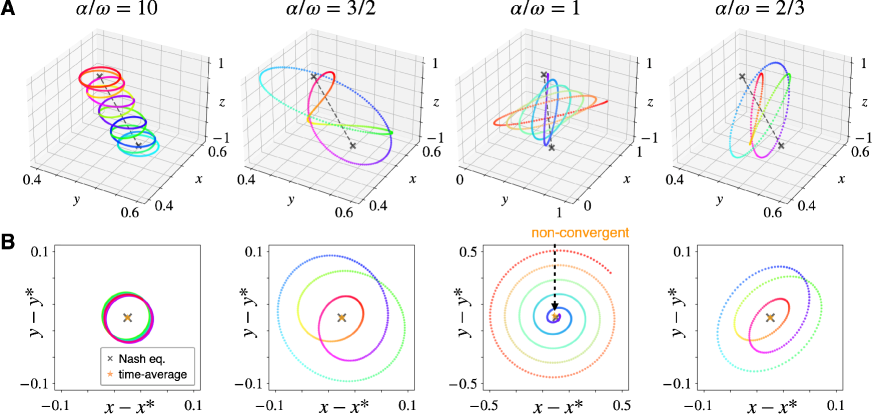
Figure 1: Learning dynamics in the periodic game of matching pennies with the time-varying Nash equilibrium. (A) The trajectories of the learning dynamics. The panels show the cases of $\alpha/\omega=10$, $2/3$, $1$, and $2/3$, from left to right. In each panel, the x-, y-, z-axes indicate $x(t)$, $y(t)$, and $z(t)$, respectively. The black broken line shows the trajectory of the Nash equilibrium, i.e., $(x^{*}(t),y^{*}(t))$, and the cross markers show the edges of the oscillation of this equilibrium. In the cases of $\alpha/\omega\neq 1$, the rainbow color shows the time of a single cycle. In $\alpha/\omega=1$, the rainbow color shows the passing of time from blue to red. (B) The projection of the trajectories of Panels A to the plane of $x(t)-x^{*}(t)$ and $y(t)-y^{*}(t)$. In each panel, the black cross marker shows the projection of the Nash equilibrium. The color corresponds to that of Panels A. The orange star markers show the time-average value of the plotted trajectory. The value does not correspond to the equilibrium in $\alpha/\omega=1$. Otherwise, it corresponds.

3.2 Solution of learning dynamics

The learning dynamics, Eqs. (13) and (14), are solvable. In the case of $\alpha/\omega=1$, the solution is

$$x(t) =\bar{x}^{*}+\frac{1}{2}\Delta x^{*}(\omega t\sin\omega t+\cos\omega t)$$

$$\hskip 8.5359pt-\frac{1}{2}\Delta y^{*}\omega t\cos\omega t+c_{1}\cos\alpha t+c_{2}\sin\alpha t,$$ (15)

$$y(t) =\bar{y}^{*}+\frac{1}{2}\Delta y^{*}(\omega t\sin\omega t+\cos\omega t)$$

$$\hskip 8.5359pt+\frac{1}{2}\Delta x^{*}\omega t\cos\omega t+c_{2}\cos\alpha t-c_{1}\sin\alpha t,$$ (16)

where $c_{1}$ and $c_{2}$ are uniquely determined by the initial state condition (see Appendix A.3 for the detailed expression of $c_{1}$ and $c_{2}$). This solution means that $x(t)$ and $y(t)$ diverges from the average Nash equilibrium $(\bar{x}^{*},\bar{y}^{*})$ at a speed of $\sqrt{|\Delta x^{*}|^{2}+|\Delta y^{*}|^{2}}\omega/2$.

On the other hand, in the case of $\alpha/\omega\neq 1$, the solution is

$$x(t) =\bar{x}^{*}+\frac{\alpha^{2}}{\alpha^{2}-\omega^{2}}\Delta x^{*}\cos\omega t+\frac{\alpha\omega}{\alpha^{2}-\omega^{2}}\Delta y^{*}\sin\omega t$$

$$\hskip 8.5359pt+c_{1}\cos\alpha t+c_{2}\sin\alpha t,$$ (17)

$$y(t) =\bar{y}^{*}+\frac{\alpha^{2}}{\alpha^{2}-\omega^{2}}\Delta y^{*}\cos\omega t-\frac{\alpha\omega}{\alpha^{2}-\omega^{2}}\Delta x^{*}\sin\omega t$$

$$\hskip 8.5359pt+c_{2}\cos\alpha t-c_{1}\sin\alpha t.$$ (18)

Here, $x(t)$ and $y(t)$ consist of two periodic solutions with the frequencies of $\alpha$ and $\omega$. Thus, the solution qualitatively changes depending on whether $\alpha/\omega=1$ or $\neq 1$.

3.3 Time-average analysis

Under fixed zero-sum payoff matrices, the dynamics of GDA are known to converge to the Nash equilibrium (called time-average convergence). We now discuss time-average convergence under periodic payoff matrices. The time-average of X’s strategy until time $T>0$ is defined as

$$\bar{x}(T):=\frac{1}{T}\int_{0}^{T}x(t){\rm d}t.$$ (19)

Interestingly, depending on $\alpha/\omega=1$ or $\neq 1$, the time-average has different properties as shown in the following. See Appendix B.1-B.4 for the full version of all the theorems.

Theorem 1 (Time-average cycling in $\alpha/\omega=1$).

In the eigenvalue invariant games, when $\alpha/\omega=1$ holds, $\bar{x}(T)$ and $\bar{y}(T)$ cycle around the Nash equilibrium.

Proof sketch. This theorem is proved by directly calculating the integral of Eqs. (15) and (16). Intuitively, since the solution diverges as it oscillates, its time-average is influenced by $x(t)$ of large time $t\simeq T$ and never converges. ∎

Theorem 2 (Time-average convergence in $\alpha/\omega\neq 1$).

In the eigenvalue invariant games, when $\alpha/\omega\neq 1$ holds, $\bar{x}(T)$ and $\bar{y}(T)$ converge to the Nash equilibrium.

Proof sketch. This theorem is proved by directly calculating the integral of Eqs. (17) and (18). In its integral, each oscillation of $\alpha$ and $\omega$ is canceled out. ∎

3.4 Visualization and interpretation

Let us visualize the learning dynamics (see Fig. 1) and interpret their behavior. This section focuses on a periodic game formulated by $\bar{\bm{U}}=((1,-1),(-1,1))$ and $\Delta\bm{U}=((1/10,0),(0,-1/10))$ in Exm. 1. Here, $\bar{\bm{U}}$ shows matching pennies with the only equilibrium of $(\bar{x}^{*},\bar{y}^{*})=(1/2,1/2)$. This periodic game has a time-invariant eigenvalue of $\alpha=2$. However, its Nash equilibrium oscillates with the amplitude of $(\Delta x^{*},\Delta y^{*})=(-1/40,-1/40)$.

First, let us see the case of $\alpha/\omega=10$. This case roughly means that players learn ten times faster than the game changes. In other words, it approximately corresponds to a classical situation where a game is time-invariant. Thus, the learning dynamics are also approximated to the classical dynamics, where the strategies of both players almost cycle around the Nash equilibrium.

Next, we see the case of $\alpha/\omega=3/2$, where the speed of game change is comparable to that of learning, but not the same. In this case, the learning interacts with the game change and provides complex dynamics (see Panel A). Although the trajectory cycles around the Nash equilibrium many times, the distance from the Nash equilibrium gets closer and farther as the equilibrium moves. After a while, the trajectory returns to its initial state and thus is periodic as described by Eqs. (17) and (18). In addition, the average of the trajectory corresponds to the equilibrium (see Panel B). The above also holds for the case when the game changes faster than the players learn (e.g., $\alpha/\omega=2/3$ in the panels).

Finally, let us focus on the case of $\alpha/\omega=1$, where the speed of game change is equal to that of learning. In other words, the cycling behavior by learning completely synchronizes the oscillation of the game. Thus, each time the game oscillates once, the amplitude of the cycle is amplified a little (see Panel A). By this amplification accumulated, the trajectory diverges from the Nash equilibrium as expressed in Eqs. (15) and (16). Furthermore, the average of the trajectory does not correspond to the Nash equilibrium.

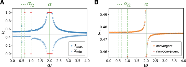
Figure 2: Experiments for learning dynamics in the eigenvalue invariant game for $\bar{\bm{U}}=((1.1,-1),(-1,0.9))$, $\Delta\bm{U}=((0.2,0),(0,0))$ without the constraint of their eigenvalues fixed. (A) The maximum (circle) and minimum (cross) values of $x(t)$ within $0\leq t\leq T=3\times 10^{4}$. Here, the blue markers indicate that the value exists in the interior of $[0,1]$, while the red exterior. (B) The time-average $\bar{x}(T)$ for the last $300$ time of $T=3\times 10^{4}$ (truncated from $0.455$ to $0.495$). The orange marker is plotted when the time-average converges, i.e., the difference between the maximum and minimum values of $\bar{x}(T)$ is smaller than $10^{-3}$. The red marker means that the time-average does not converge. The gray broken line shows the analytical solution.

4 Theory on eigenvalue varying games

We now extend the insight obtained from the eigenvalue invariant game (i.e., Exm. 1) to more general settings. The eigenvalue invariant game is extended in two points: 1) its eigenvalue time-varying and 2) the shape of the wave.

Definition 2 ($2\times 2$ smooth periodic games).

$2\times 2$ smooth periodic games are defined as any smooth $\{\bm{U}(t)\}_{0\leq t<2\pi/\omega}\in\mathbb{R}^{2\times 2}\times[0,2\pi/\omega)$, satisfying $\bm{U}(t)=\bm{U}(t+2\pi/\omega)$.

4.1 Solution of learning dynamics

Below, we use the notation of

$$2f(t) :=u_{11}(t)-u_{12}(t)-u_{21}(t)+u_{22}(t),$$ (20)

$$2g(t) :=-u_{12}(t)+u_{22}(t),$$ (21)

$$2h(t) :=-u_{21}(t)+u_{22}(t).$$ (22)

All of these functions are periodic with frequency $\omega$. Here, we see that $f(t)$ represents the eigenvalue of learning and varies over time. By using these equations, we describe the learning dynamics in Def. 2 as

$$\dot{x}(t) =+f(t)y(t)-g(t),$$ (23)

$$\dot{y}(t) =-f(t)x(t)+h(t).$$ (24)

These simultaneous differential equations are solved as

$$x(t) =\int_{0}^{t}h(\tau)\sin(F(t)-F(\tau)){\rm d}\tau$$

$$\hskip 8.5359pt-\int_{0}^{t}g(\tau)\cos(F(t)-F(\tau)){\rm d}\tau$$

$$\hskip 8.5359pt+c_{1}\cos F(t)+c_{2}\sin F(t),$$ (25)

$$y(t) =\int_{0}^{t}g(\tau)\sin(F(t)-F(\tau)){\rm d}\tau$$

$$\hskip 8.5359pt+\int_{0}^{t}h(\tau)\cos(F(t)-F(\tau)){\rm d}\tau$$

$$\hskip 8.5359pt+c_{2}\cos F(t)-c_{1}\sin F(t).$$ (26)

Here, $c_{1}$ and $c_{2}$ are uniquely determined by the initial state condition (see Appendix A.4 for detailed expression of $c_{1}$ and $c_{2}$). In addition, we defined $F(t):=\int_{0}^{t}f(\tau){\rm d}\tau$. This $F(t)$ is not periodic, but other than the linear term $\Delta F(t):=F(t)-\bar{f}t$ is periodic with frequency $\omega$. This linear term corresponds to the average eigenvalue, i.e., $\alpha=\bar{f}$.

4.2 Time-average analysis

Let us analyze the time-average of the learning dynamics, i.e., Eqs. (25) and (26). Since we assume general smooth periodic functions for $f$, $g$, and $h$, we cannot analytically calculate the integral of $x(t)$, as different from the case of Exm. 1. Thus, we have to devise a way to evaluate $x(T)$ (see the following proof sketch for details). Now, when $\alpha/\omega\in\mathbb{N}$ holds, we prove that the time-average diverges generically (see Appendix C for some exceptions).

Theorem 3 (Time-average divergence in $\alpha/\omega\in\mathbb{N}$).

In two-action periodic zero-sum games, when $\alpha/\omega\in\mathbb{N}$, $\bar{x}(T)$ and $\bar{y}(T)$ diverge over time $T$.

Proof sketch. As different from the proofs of Thms. 1 and 2, the integral of the trajectory (Eqs. (25) and (26)) cannot be calculated directly. In the case of $\alpha/\omega\in\mathbb{N}$, however, we can easily evaluate the time-average by paying attention to the periodicity of $\sin F(\cdot)$ and $\cos F(\cdot)$ with frequency $\omega$. We divide the ranges of integrals, i.e., $t\in[0,T]$ and $\tau\in[0,t]$, into the intervals of $2\pi/\omega$, and the time-average is also divided into the following four terms: 1) the term of diverges which is $O(T)$ in the time-average, 2) the term oscillates which is $O(1)$, the term converges which is $O(1)$, and 4) the term is negligible which is $O(1/T)$. In general functions, $f$, $g$, and $h$, the divergence term takes a finite value, and thus we prove that the time-average is $O(T)$ and thus diverges with time. ∎

Otherwise, the time-average converges as follows.

Theorem 4 (Time-average convergence in $\alpha/\omega\notin\mathbb{N}$).

In two-action periodic zero-sum games, when $\alpha/\omega\notin\mathbb{N}$, $\bar{x}(T)$ and $\bar{y}(T)$ converge over time $T$.

Proof sketch. We consider the same division of the ranges of the integrals as proof of Thm. 3 and evaluate the four terms. In the case of $\alpha/\omega\notin\mathbb{N}$, however, this evaluation is much more difficult because we cannot generally use the periodicity of $\sin F(\cdot)$ and $\cos F(\cdot)$. By utilizing a property of the non-periodicity, the divergence term falls into $O(1)$, while the oscillation term into $O(1/T)$. Thus, the time-average converges with neither divergence nor oscillation. ∎

Figure 3: Learning dynamics in a three-action periodic game. We use an example of $\bm{U}(t)=\bar{\bm{U}}+\bm{A}_{1}\cos\omega t+\bm{A}_{2}\cos 2\omega t+\bm{B}_{1}\sin\omega t+\bm{B}_{2}\sin 2\omega t$ with $\bar{\bm{U}}=((0,-1,3),(2,0,-1),(-4,1,0))$, $\bm{A}_{1}=((16,-6,-5),(-11,9,-23),(17,-8,3))\times 10^{-2}$, $\bm{B}_{1}=((-2,15,-21),(-3,-4,11),(-11,-2,-9)\times 10^{-2}$, $\bm{A}_{2}=((0,6,-11),(11,9,5),(9,-7,-1))\times 10^{-2}$, $\bm{B}_{2}=((-9,-3,5),(-7,-4,-7),(-8,-7,0))\times 10^{-2}$. The only Nash equilibrium of $\bar{\bm{U}}$ is $\bm{x}^{*}=(1/5,19/35,9/35)$ and $\bm{y}^{*}=(1/7,22/35,8/35)$. (A) The maximum value of $x_{1}(t)$ for sufficiently large $t$. The meanings of the markers and axes are the same as Fig. 2-A. (B) The average value of $\bar{x}_{1}(T)$ for sufficiently large $T$. The meanings of the markers and axes are the same as Fig. 2-B.

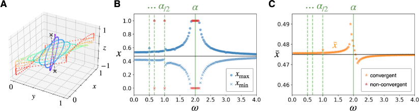
Figure 4: Learning dynamics under the boundary constraint of Eqs. (1) and (2). All the parameters of the game and data are the same as Fig. 2. (A) The trajectory of learning dynamics in $\omega=\alpha$. The meanings of plots and axes are the same as Fig. 1-A. (B) The maximum value of $x(t)$ for sufficiently large $t$. The meanings of the markers and axes are the same as Fig. 2-A. (C) The average value of $\bar{x}_{1}(T)$ for sufficiently large $T$. The meanings of the markers and axes are the same as Fig. 2-B.

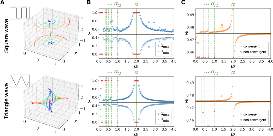
Figure 5: Learning dynamics for non-smooth game changes. The upper panels show square waves, while the lower panels show triangle waves. All the parameters of the game and data are the same as Fig. 2. (A) The trajectory of learning dynamics in $\omega=\alpha$. The meanings of plots and axes are the same as Fig. 1-A. (B) The maximum value of $x(t)$ for sufficiently large $t$. The meanings of the markers and axes are the same as Fig. 2-A. (C) The average value of $\bar{x}_{1}(T)$ for sufficiently large $T$. The meanings of the markers and axes are the same as Fig. 2-B.

4.3 Experimental verification for theory

Let us see that Thms. 3 and 4 hold in experiments. It is enough to simply extend Exm. 1 not to satisfy the constraint for $\Delta\bm{U}$, and we use the example of $\bar{\bm{U}}=((1.1,-1),(-1,0.9))$ and $\Delta\bm{U}=((0.2,0),(0,0))$. This example is calculated as $f(t)=2+0.1\cos\omega t$ and $g(t)=h(t)=0.95$, showing that not only the Nash equilibrium but the eigenvalue oscillates. Fig. 2 shows comprehensive experiments for various $\omega$. These experiments are based on the fourth-order Runge-Kutta method with step size $1/40$ for time $0\leq t\leq 3\times 10^{5}$. The initial strategies are set to the Nash equilibrium of the time-average game, i.e., $x(0)=\bar{h}/\bar{f}$, $y(0)=\bar{g}/\bar{f}$.

First, Panel A shows the maximum and minimum values of $x(t)$ for the whole $t$. We see that $x(t)$ always continues to oscillate. Especially in $\alpha/\omega\in\mathbb{N}$, the amplitude of this oscillation is large. Elsewhere, the amplitude is small.

Next, Panel B shows the time-average $\bar{x}(T)$ for sufficiently large $T$. We observe that the time-average diverges in $\alpha/\omega\in\mathbb{N}$, reflecting Thm. 3. Here, however, note that when $\alpha/\omega$ takes a sufficiently large integer ($\alpha/\omega\geq 3$ in the panel), the divergence is weak and judged to be convergent. The time-average converges in $\alpha/\omega\notin\mathbb{N}$, reflecting Thm. 4.

5 Experimental results

So far, for theoretical analyses, we have focused on an idealized situation 1) of two-action games, 2) without the boundary of the players’ strategy spaces, and 3) with smoothness in the periodicity. In the following, we perform experiments of learning in periodic games without such an idealization. The above insight, i.e., the qualitative difference of learning dynamics depending on whether the synchronization occurs or not, is universal and independent of these idealizations. We basically use the same method and parameters as Fig. 2. The only exception is the experiments in Fig. 4, where the time step is $1/(4\times 10^{3})$ for $0\leq t\leq 10^{4}$ because the dynamics are sensitive in the boundary of the strategy spaces.

5.1 Various action numbers

Extensively, we consider a three-action periodic game, a weighted rock-paper-scissors game with the payoff matrix slightly vibrating following several circular functions. Thus, the Nash equilibrium always exists in the interior of the simplexes but oscillates in a complex way. Let us see the properties beyond those of two-action games. First, as the dimension of the payoff matrix increases, the number of the eigenvalues increases. In Fig. 3, the two eigenvalues, $\alpha^{(1)}>\alpha^{(2)}>1$, are plotted as the pink and green lines. In $\alpha^{(i)}/\omega\in\mathbb{N}$ and its neighbor, one’s strategy oscillates with a large amplitude (see Panel A), and its time-average tends to diverge (see Panel B). Otherwise, the time-average converges to near the Nash equilibrium.

5.2 Boundary constraint

Next, we consider the boundary constraint given by the Euclidean regularizer in Eqs. (1) and (2). The learning dynamics are different from Eqs. (3) only on the boundary of the strategy spaces, i.e., $x,y\in\{0,1\}$ (see Panel A). Despite the existence of the boundary constraint, in $\alpha/\omega\in\mathbb{N}$ and its neighbor, one’s strategy oscillates with a large amplitude (see Panel B). Elsewhere, the amplitude is small. However, since the amplitude is bounded by the boundary constraint, the time-average of one’s strategy always converges, even in $\alpha/\omega\in\mathbb{N}$ (see Panel C).

5.3 Non-smooth periodicity

Finally, Fig. 5 shows the experiment for some non-smooth game changes. The upper panels show a square wave, which is a discontinuous function of $t$, while the lower ones show a triangle wave, which is a non-differentiable function (see Panels A for examples of typical trajectories). A similar result holds to the smooth periodic games (compare Panels B and C with Fig. 2). The only difference is that one’s strategy and its time-average are more likely to diverge when $\alpha/\omega$ takes a large integer (see the left sides of Panels B and C). This is probably because the square and triangle waves have an infinite number of frequency components, i.e., $\omega,2\omega,\cdots$.

6 Conclusion

This study examined learning in periodic games where the Nash equilibrium is time-varying. We discussed the dynamics of learning and their time-average convergence/non-convergence. Notably, this study focused on the synchronization of learning with the periodic change of games. We identified a phenomenon where the learning dynamics qualitatively change depending on whether the synchronization occurs or not. When the synchronization occurs, learning dynamics diverge from the Nash equilibrium, and their time average does not converge. Otherwise, the dynamics enter a complex cycle, but their time-average converges. We proved this phenomenon in a wide range of games, but with a limitation of two-action, the smooth periodicity of the game, and the absence of the boundary constraint of the strategy space. Our experiments demonstrated that this phenomenon universally occurs, regardless of these limitations.

One of the remained problems is that the time-average converges elsewhere than the Nash equilibrium of the game’s time-average. This problem is contrary to classical time-invariant games but consistent with (Fiez et al. 2021). As a future work, it would be interesting to consider how to track the time-varying Nash equilibrium or converge to the Nash equilibrium of the time-average of periodic games. Another problem is to see and analyze the learning dynamics of other algorithms, such as optimistic (Rakhlin and Sridharan 2013; Syrgkanis et al. 2015; Daskalakis et al. 2018; Daskalakis and Panageas 2019; Cai, Oikonomou, and Zheng 2022), extra-gradient (Korpelevich 1976; Mertikopoulos et al. 2019; Lee and Kim 2021; Cai, Oikonomou, and Zheng 2022), and negative momentum (Polyak 1964; Gidel et al. 2019; Kovachki and Stuart 2021; Zhang and Wang 2021; Hemmat et al. 2023), all of which are known to converge of the strategies themselves to the Nash equilibrium, called last-iterate convergence. The behavior of such algorithms is already known under periodic games when the Nash equilibrium does not move (Feng et al. 2023, 2024), but not when moves. In addition, it would be interesting to extend two-player zero-sum games into the poly-matrix games (Bergman and Fokin 1998; Cai and Daskalakis 2011; Bailey and Piliouras 2019), which are $n$-player games divisible into $2$-player zero-sum interactions. How synchronization occurs when the poly-matrix game includes two games equipped with different eigenvalues is a non-trivial theme. This study finds a new phenomenon in learning in periodic games and gives insight into the phenomenon, providing a theoretical basis for these future problems.

Appendix

Appendix A Derivation of equations

A.1 Derivation of gradient descent-ascent dynamics

This section is dedicated to deriving the continuous form of the gradient descent-ascent, i.e., Eq. (1). First, in the argument of minimum, the extreme condition is satisfied as

$$\bm{x}^{\dagger}-\bm{x}=c\bm{1}_{\sf X}.$$ (A1)

Here, from the constraint of $\bm{x}\in\Delta^{m_{\sf X}-1}$, $c$ is calculated as

$$\bm{1}_{\sf X}^{\rm T}\bm{x}^{\dagger}-\underbrace{\bm{1}_{\sf X}^{\rm T}\bm{x}}_{=1}=c\underbrace{\bm{1}_{\sf X}^{\rm T}\bm{1}_{\sf X}}_{=m_{\sf X}}\quad\Leftrightarrow c=\frac{1}{m_{\sf X}}(\bm{1}_{\sf X}^{\rm T}\bm{x}^{\dagger}-1).$$ (A2)

By substituting this equation, we obtain

$$\bm{x} =\bm{x}^{\dagger}-\frac{\bm{1}_{\sf X}}{m_{\sf X}}(\bm{1}_{\sf X}^{\rm T}\bm{x}^{\dagger}-1)=\bm{P}_{\sf X}\bm{x}^{\dagger}+\frac{\bm{1}_{\sf X}}{m_{\sf X}}.$$ (A3)

Finally, its time derivative is

$$\dot{\bm{x}}=\bm{P}_{\sf X}\dot{\bm{x}}^{\dagger}=\bm{P}_{\sf X}\bm{U}\bm{y}.$$ (A4)

In a similar way (replace $\bm{P}_{\sf X}$ with $\bm{P}_{\sf Y}$ and $\bm{U}\bm{y}$ with $-\bm{U}^{\rm T}\bm{x}$), we calculate $\dot{\bm{y}}$ as

$$\dot{\bm{y}}=-\bm{P}_{\sf Y}\bm{U}^{\rm T}\bm{x}.$$ (A5)

By combining these equations, we obtain Eq. (3).

A.2 Derivation of eigenvalues in two-action games

$$\bm{P}_{\sf X}\bm{U}\bm{P}_{\sf Y}\bm{U}^{\rm T} =\frac{1}{4}\begin{pmatrix}+1&-1\\ -1&+1\\ \end{pmatrix}\begin{pmatrix}u_{11}(t)&u_{12}(t)\\ u_{21}(t)&u_{22}(t)\\ \end{pmatrix}\begin{pmatrix}+1&-1\\ -1&+1\\ \end{pmatrix}\begin{pmatrix}u_{11}(t)&u_{21}(t)\\ u_{12}(t)&u_{22}(t)\\ \end{pmatrix}$$

$$=\frac{1}{4}(u_{11}(t)-u_{12}(t)-u_{21}(t)+u_{22}(t))\begin{pmatrix}+1\\ -1\\ \end{pmatrix}\otimes\begin{pmatrix}u_{11}(t)-u_{21}(t)\\ u_{12}(t)-u_{22}(t)\\ \end{pmatrix}$$ (A6)

Thus, by the tensor product representation of $\bm{P}_{\sf X}\bm{U}\bm{P}_{\sf Y}\bm{U}^{\rm T}$, the eigenvalues are trivially obtained as

$$\det(\lambda^{2}\bm{I}_{\sf X}+\bm{P}_{\sf X}\bm{U}\bm{P}_{\sf Y}\bm{U}^{\rm T})=0$$

$$\Leftrightarrow\lambda^{2}=-\frac{1}{4}(u_{11}(t)-u_{12}(t)-u_{21}(t)+u_{22}(t))^{2},\ 0$$

$$\Leftrightarrow\lambda=\pm i\frac{1}{2}(u_{11}(t)-u_{12}(t)-u_{21}(t)+u_{22}(t)),\ \pm 0.$$ (A7)

In addition, the eigenvalue of learning is described as

$$\alpha^{(1)} =\frac{1}{2}(\bar{u}_{11}-\bar{u}_{12}-\bar{u}_{21}+\bar{u}_{22}),$$ (A8)

$$\alpha^{(2)} =0,$$ (A9)

which correspond to Eqs. (9) and (10).

A.3 Derivation of Eqs. (15) and (18)

In Eqs. (17) and (18), where $\alpha\neq\omega$ is assumed, $c_{1}$ and $c_{2}$ are uniquely determined by the initial state condition as

$$c_{1}=x(0)-\bar{x}^{*}-\frac{\alpha^{2}}{\alpha^{2}-\omega^{2}}\Delta x^{*},\quad c_{2}=y(0)-\bar{y}^{*}-\frac{\alpha^{2}}{\alpha^{2}-\omega^{2}}\Delta y^{*}.$$ (A10)

In the limit of $\alpha\to\omega$, $c_{1}$ and $c_{2}$ uniquely exist as

$$\lim_{\alpha\to\omega}\frac{\alpha^{2}}{\alpha^{2}-\omega^{2}}=\frac{1}{2}.$$ (A11)

This limit solves the initial value problem in the case of $\alpha=\omega$, i.e., Eqs. (15) and (16).

A.4 Derivation of Eqs. (25) and (26)

In this section, we see that Eqs. (25) and (26) are the solution of Eqs. (23) and (24). First, we only con

$$\dot{x}(t) =h(t)\underbrace{\sin(F(t)-F(t))}_{=0}+f(t)\int_{0}^{t}h(\tau)\cos(F(t)-F(\tau)){\rm d}\tau-g(t)\underbrace{\cos(F(t)-F(t))}_{=1}+f(t)\int_{0}^{t}g(\tau)\sin(F(t)-F(\tau)){\rm d}\tau$$

$$\hskip 8.5359pt-f(t)c_{1}\sin F(t)+f(t)c_{2}\cos F(t)$$

$$=+f(t)\underbrace{\left(\int_{0}^{t}g(\tau)\sin(F(t)-F(\tau)){\rm d}\tau+\int_{0}^{t}h(\tau)\cos(F(t)-F(\tau)){\rm d}\tau+c_{2}\cos F(t)-c_{1}\sin F(t)\right)}_{=y(t)}-g(t)$$

$$=+f(t)y(t)-g(t),$$ (A12)

$$\dot{y}(t) =g(t)\underbrace{\sin(F(t)-F(t))}_{=0}+f(t)\int_{0}^{t}g(\tau)\cos(F(t)-F(\tau)){\rm d}\tau+h(t)\underbrace{\cos(F(t)-F(t))}_{=1}-f(t)\int_{0}^{t}h(\tau)\sin(F(t)-F(\tau)){\rm d}\tau$$

$$\hskip 8.5359pt-f(t)c_{2}\sin F(t)-f(t)c_{1}\cos F(t)$$

$$=-f(t)\underbrace{\left(\int_{0}^{t}h(\tau)\sin(F(t)-F(\tau)){\rm d}\tau-\int_{0}^{t}g(\tau)\cos(F(t)-F(\tau)){\rm d}\tau+c_{1}\cos F(t)+c_{2}\sin F(t)\right)}_{=x(t)}+h(t)$$

$$=-f(t)x(t)+h(t).$$ (A13)

We also determine $c_{1}$ and $c_{2}$ by the initial state condition of $x(0)$ and $y(0)$ as

$$c_{1}=x(0)\cos F(0)-y(0)\sin F(0),\quad c_{2}=y(0)\cos F(0)+x(0)\sin F(0).$$ (A14)

Appendix B Proofs

B.1 Proof of Theorem 1

Proof.

From Eq. (15), we derive $\bar{x}(T)$ as

$$\bar{x}(T) =\frac{1}{T}\int_{0}^{T}\bar{x}^{*}+\frac{1}{2}\Delta x^{*}(\omega t\sin\omega t+\cos\omega t)-\frac{1}{2}\Delta y^{*}\omega t\cos\omega t+c_{1}\cos\omega t+c_{2}\sin\omega t{\rm d}t$$

$$=\frac{1}{T}\left[\bar{x}^{*}t-\frac{1}{2}\Delta x^{*}\left(t\cos\omega t-\frac{2}{\omega}\sin\omega t\right)-\frac{1}{2}\Delta y^{*}\left(t\sin\omega t+\frac{1}{\omega}\cos\omega t\right)+\frac{c_{1}}{\omega}\sin\omega t-\frac{c_{2}}{\omega}\cos\omega t\right]_{0}^{T}$$

$$=\bar{x}^{*}-\left(\frac{1}{2}\Delta x^{*}\cos\omega T+\frac{1}{2}\Delta y^{*}\sin\omega T\right)+O(T^{-1}).$$ (A15)

In the same way, we derive $\bar{y}(T)$ as

$$\bar{y}(T) =\bar{y}^{*}-\left(\frac{1}{2}\Delta y^{*}\cos\omega T-\frac{1}{2}\Delta x^{*}\sin\omega T\right)+O(T^{-1}).$$ (A16)

Thus, both $\bar{x}(T)$ and $\bar{y}(T)$ no converge with $T\to\infty$ and continue to oscillate. ∎

B.2 Proof of Theorem 2

Proof.

From Eq. (17), we derive $\bar{x}(T)$ as

$$\bar{x}(T) =\frac{1}{T}\int_{0}^{T}\bar{x}^{*}+\frac{\alpha^{2}}{\alpha^{2}-\omega^{2}}\Delta x^{*}\cos\omega t+\frac{\alpha\omega}{\alpha^{2}-\omega^{2}}\Delta y^{*}\sin\omega t+c_{1}\cos\alpha t+c_{2}\sin\alpha t{\rm d}t$$

$$=\frac{1}{T}\left[\bar{x}^{*}t+\frac{\alpha^{2}}{\omega(\alpha^{2}-\omega^{2})}\Delta x^{*}\sin\omega t-\frac{\alpha}{\alpha^{2}-\omega^{2}}\Delta y^{*}\cos\omega t+\frac{c_{1}}{\alpha}\sin\alpha t-\frac{c_{2}}{\alpha}\cos\alpha t\right]_{0}^{T}$$

$$=\bar{x}^{*}+O(T^{-1}).$$ (A17)

Thus, we obtain $\lim_{T\to\infty}\bar{x}(T)=\bar{x}^{*}$. In the same way, we can prove $\lim_{T\to\infty}\bar{y}(T)=\bar{y}^{*}$. ∎

B.3 Proof of Theorem 3

Proof.

We denote $\alpha/\omega=n\in\mathbb{N}$. Note that by definition, we need to calculate double integrals for $t$ and $\tau$ in order to derive the time-average $\bar{x}(T)$. The ranges of integrals, i.e., $t\in[0,T]$ and $\tau\in[0,t]$, are divided by the intervals of $2\pi/\omega$ (see Fig. 1). We define

$$\mu(T):=\left\lfloor\frac{\omega T}{2\pi}\right\rfloor,\quad\nu(T):=T-\frac{2\pi}{\omega}\mu(T).$$ (A18)

Here, $\mu(T)$ is the number of the intervals and is $O(T)$, while $\nu(T)$ is the remainder and is $O(1)$. Thus, $T=2\pi\mu(T)/\omega+\nu(T)$ holds.

Now, we describe the integral of the first term in Eq. (25) as

$$\int_{0}^{T}\int_{0}^{t}h(\tau)\sin(F(t)-F(\tau)){\rm d}\tau{\rm d}t$$

$$=\sum_{l=0}^{\mu(T)-1}\sum_{k=0}^{l-1}\int_{\frac{2\pi}{\omega}l}^{\frac{2\pi}{\omega}(l+1)}\int_{\frac{2\pi}{\omega}k}^{\frac{2\pi}{\omega}(k+1)}h(\tau)\sin(F(t)-F(\tau)){\rm d}\tau{\rm d}t+\int_{\frac{2\pi}{\omega}\mu(T)}^{\frac{2\pi}{\omega}\mu(T)+\nu(T)}\sum_{k=0}^{\mu(T)-1}\int_{\frac{2\pi}{\omega}k}^{\frac{2\pi}{\omega}(k+1)}h(\tau)\sin(F(t)-F(\tau)){\rm d}\tau{\rm d}t$$

$$\hskip 8.5359pt+\sum_{l=0}^{\mu(T)-1}\int_{\frac{2\pi}{\omega}l}^{\frac{2\pi}{\omega}(l+1)}\int_{\frac{2\pi}{\omega}l}^{\frac{2\pi}{\omega}l+\nu(t)}h(\tau)\sin(F(t)-F(\tau)){\rm d}\tau{\rm d}t+\int_{\frac{2\pi}{\omega}\mu(T)}^{\frac{2\pi}{\omega}\mu(T)+\nu(T)}\int_{\frac{2\pi}{\omega}\mu(T)}^{\frac{2\pi}{\omega}\mu(T)+\nu(t)}h(\tau)\sin(F(t)-F(\tau)){\rm d}\tau{\rm d}t$$ (A19)

$$=\frac{\mu(T)(\mu(T)-1)}{2}\int_{0}^{\frac{2\pi}{\omega}}\int_{0}^{\frac{2\pi}{\omega}}h(\tau)\sin(F(t)-F(\tau)){\rm d}\tau{\rm d}t+\mu(T)\int_{0}^{\frac{2\pi}{\omega}}\int_{0}^{t}h(\tau)\sin(F(t)-F(\tau)){\rm d}\tau{\rm d}t$$

$$\hskip 8.5359pt+\mu(T)\int_{0}^{\nu(T)}\int_{0}^{\frac{2\pi}{\omega}}h(\tau)\sin(F(t)-F(\tau)){\rm d}\tau{\rm d}t+\int_{0}^{\nu(T)}\int_{0}^{t}h(\tau)\sin(F(t)-F(\tau)){\rm d}\tau{\rm d}t.$$ (A20)

Here, in the first equality, we divided the ranges of the integrals. In the second equality, we used the periodicity of $h(\tau)\sin(F(t)-F(\tau))$. In other words, $h(\tau)\sin(F(t)-F(\tau))$ is invariant about the transforms of $t\to t+\frac{2\pi}{\omega}l$ and $\tau\to\tau+\frac{2\pi}{\omega}k$ for all $k,l\in\mathbb{N}$ as

$$h(\tau+\frac{2\pi}{\omega}k)\sin(F(t+\frac{2\pi}{\omega}l)-F(\tau+\frac{2\pi}{\omega}k)) =h(\tau)\sin(F(t)-F(\tau)+2\pi\frac{\alpha}{\omega}(l-k))$$

$$=h(\tau)\sin(F(t)-F(\tau)+2\pi n(l-k))$$

$$=h(\tau)\sin(F(t)-F(\tau)).$$ (A21)

Here, recall that $h(\cdot)$ and $\Delta F(\cdot)=F(\cdot)-\alpha t$ is periodic for frequency $\omega$.

Since $\mu(T)=O(T)$, the first term is $O(T^{2})$ and dominant. Thus, it is proved that $\bar{x}(T)$ and $\bar{y}(T)$ diverge with the speeds of

$$\lim_{T\to\infty}\frac{1}{T}\bar{x}(T) =\frac{1}{2}\left(\frac{\omega}{2\pi}\right)^{2}\int_{0}^{\frac{2\pi}{\omega}}\int_{0}^{\frac{2\pi}{\omega}}h(\tau)\sin(F(t)-F(\tau))-g(\tau)\cos(F(t)-F(\tau)){\rm d}\tau{\rm d}t,$$ (A22)

$$\lim_{T\to\infty}\frac{1}{T}\bar{y}(T) =\frac{1}{2}\left(\frac{\omega}{2\pi}\right)^{2}\int_{0}^{\frac{2\pi}{\omega}}\int_{0}^{\frac{2\pi}{\omega}}g(\tau)\sin(F(t)-F(\tau))+h(\tau)\cos(F(t)-F(\tau)){\rm d}\tau{\rm d}t.$$ (A23)

Interpretation of each term:

Let us interpret the meaning of Eqs. (A19) by Fig. 1. The first terms of Eqs. (A19) correspond to the red area of the figure, and the area is $O(T^{2})$. By considering the average for $T$, its time-average is $O(T)$, thus called the “divergence” term. Next, the second terms correspond to the green area, and the area is $O(T)$. Thus, its time-average is $O(1)$. This area is also proportional to $\nu(T)$ and thus oscillates with frequency $\omega$, called the “oscillation” term. Next, the third terms correspond to the blue area, and the area is $O(T)$. Thus, its time-average is $O(1)$. Because this area converges to a value in the limit of $T\to\infty$, we call it the “convergence” term. Finally, the fourth terms correspond to the orange area, and the area is $O(1)$. Thus, its time-average is $O(1/T)$ and thus becomes negligible over time, called the “negligible” term.

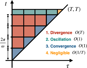
Figure A 1: Schematics of the division of integral ranges. The x- and y-axes indicate the direction of $\tau$ and $t$, respectively. All the colored area (i.e., $0\leq\tau\leq t\leq T$) shows the range of integral. Each square is of length $2\pi/\omega$. (1) The red area shows the divergence term, which is $O(T)$ in the time-average and thus diverges. (2) The green area shows the oscillation term, which is $O(1)$ in the time-average and oscillates over time. (3) The blue area shows the convergence term, which is $O(1)$ in the time-average. (4) Last, the orange area shows the negligible term, which is $O(1/T)$ in the time-average and thus disappears over time.

∎

B.4 Proof of Theorem 4

Proof.

We consider the case of $\alpha/\omega=r\in\mathbb{R}\setminus\mathbb{N}$. In this case, we divide the ranges of the integrals, i.e., $t\in[0,T]$ and $\tau\in[0,t]$, by the intervals of $2\pi/\omega$, again. We define the number of intervals $\mu(T)$ and the remainder $\nu(T)$ as

$$\mu(T):=\left\lfloor\frac{\omega T}{2\pi}\right\rfloor,\quad\nu(T):=T-\frac{2\pi}{\omega}\mu(T).$$ (A24)

The third term of Eq. (25) is calculated as

$$\int_{0}^{T}\int_{0}^{t}h(\tau)\sin(F(t)-F(\tau)){\rm d}\tau{\rm d}t$$

$$=\underbrace{\sum_{l=0}^{\mu(T)-1}\sum_{k=0}^{l-1}\int_{\frac{2\pi}{\omega}l}^{\frac{2\pi}{\omega}(l+1)}\int_{\frac{2\pi}{\omega}k}^{\frac{2\pi}{\omega}(k+1)}h(\tau)\sin(F(t)-F(\tau)){\rm d}\tau{\rm d}t}_{=:({\rm A})}+\underbrace{\int_{\frac{2\pi}{\omega}\mu(T)}^{\frac{2\pi}{\omega}\mu(T)+\nu(T)}\sum_{k=0}^{\mu(T)-1}\int_{\frac{2\pi}{\omega}k}^{\frac{2\pi}{\omega}(k+1)}h(\tau)\sin(F(t)-F(\tau)){\rm d}\tau{\rm d}t}_{=:({\rm B})}$$

$$\hskip 8.5359pt+\underbrace{\sum_{l=0}^{\mu(T)-1}\int_{\frac{2\pi}{\omega}l}^{\frac{2\pi}{\omega}(l+1)}\int_{\frac{2\pi}{\omega}l}^{t}h(\tau)\sin(F(t)-F(\tau)){\rm d}\tau{\rm d}t}_{=:({\rm C})}+\underbrace{\int_{\frac{2\pi}{\omega}\mu(T)}^{\frac{2\pi}{\omega}\mu(T)+\nu(T)}\int_{\frac{2\pi}{\omega}\mu(T)}^{t}h(\tau)\sin(F(t)-F(\tau)){\rm d}\tau{\rm d}t}_{=O(1)}$$

$$=\frac{1}{2}\mu(T)\int_{0}^{\frac{2\pi}{\omega}}\int_{0}^{\frac{2\pi}{\omega}}h(\tau)\left(-\sin(F(t)-F(\tau))+\frac{\sin 2\pi r}{1-\cos 2\pi r}\cos(F(t)-F(\tau))\right){\rm d}\tau{\rm d}t$$

$$\hskip 8.5359pt+\mu(T)\int_{0}^{\frac{2\pi}{\omega}}\int_{0}^{t}h(\tau)\sin(F(t)-F(\tau)){\rm d}\tau{\rm d}t+O(1).$$ (A25)

Divergence term:

The term $({\rm A})$ is calculated as

$$({\rm A}) =\sum_{l=0}^{\mu(T)-1}\sum_{k=0}^{l-1}\int_{\frac{2\pi}{\omega}l}^{\frac{2\pi}{\omega}(l+1)}\int_{\frac{2\pi}{\omega}k}^{\frac{2\pi}{\omega}(k+1)}h(\tau)\sin(F(t)-F(\tau)){\rm d}\tau{\rm d}t$$

$$=\sum_{l=0}^{\mu(T)-1}\sum_{k=0}^{l-1}\int_{0}^{\frac{2\pi}{\omega}}\int_{0}^{\frac{2\pi}{\omega}}h(\tau)\sin(F(t)-F(\tau)+2\pi r(l-k)){\rm d}\tau{\rm d}t$$

$$=\sum_{l=0}^{\mu(T)-1}\sum_{k=0}^{l-1}\int_{0}^{\frac{2\pi}{\omega}}\int_{0}^{\frac{2\pi}{\omega}}h(\tau)(\sin(F(t)-F(\tau))\cos 2\pi r(l-k)+\cos(F(t)-F(\tau))\sin 2\pi r(l-k)){\rm d}\tau{\rm d}t$$

$$=\frac{1}{2}\mu(T)\int_{0}^{\frac{2\pi}{\omega}}\int_{0}^{\frac{2\pi}{\omega}}h(\tau)\left(-\sin(F(t)-F(\tau))+\frac{\sin 2\pi r}{1-\cos 2\pi r}\cos(F(t)-F(\tau))\right){\rm d}\tau{\rm d}t+O(1).$$ (A26)

Here, we used

$$\sum_{l=0}^{\mu(T)-1}\sum_{k=0}^{l-1}\cos 2\pi r(l-k)+i\sum_{l=0}^{\mu(T)-1}\sum_{k=0}^{l-1}\sin 2\pi r(l-k)=\sum_{l=0}^{\mu(T)-1}\sum_{k=0}^{l-1}e^{i2\pi r(l-k)}$$

$$=\sum_{l=0}^{\mu(T)-1}\frac{e^{i2\pi rl}-1}{1-e^{-i2\pi r}}=\frac{1}{1-e^{-i2\pi r}}\left(\frac{1-e^{i2\pi r\mu(T)}}{1-e^{i2\pi r}}-\mu(T)\right)=\frac{-1}{1-e^{-i2\pi r}}\mu(T)+O(1)$$

$$=\frac{-(1-\cos 2\pi r)+i\sin 2\pi r}{2(1-\cos 2\pi r)}\mu(T)+O(1)$$

$$\Leftrightarrow\sum_{l=0}^{\mu(T)-1}\sum_{k=0}^{l-1}\cos 2\pi r(l-k)=-\frac{1}{2}\mu(T)+O(1),\quad\sum_{l=0}^{\mu(T)-1}\sum_{k=0}^{l-1}\sin 2\pi r(l-k)=\frac{\sin 2\pi r}{2(1-\cos 2\pi r)}\mu(T)+O(1)$$ (A27)

Thus, in its time-average, the divergence term is $O(T)$ and is bounded.

Oscillation term:

The term $({\rm B})$ is also calculated as

$$({\rm B}) =\int_{\frac{2\pi}{\omega}\mu(T)}^{\frac{2\pi}{\omega}\mu(T)+\nu(T)}\sum_{k=0}^{\mu(T)-1}\int_{\frac{2\pi}{\omega}k}^{\frac{2\pi}{\omega}(k+1)}h(\tau)\sin(F(t)-F(\tau)){\rm d}\tau{\rm d}t$$

$$=\int_{\frac{2\pi}{\omega}\mu(T)}^{\frac{2\pi}{\omega}\mu(T)+\nu(T)}\sum_{k=0}^{\mu(T)-1}\int_{0}^{\frac{2\pi}{\omega}}h(\tau)\sin(F(t)-F(\tau)-2\pi rk){\rm d}\tau{\rm d}t$$

$$=O(1).$$ (A28)

Here, we used

$$\sum_{k=0}^{\mu(T)-1}\cos 2\pi rk+i\sum_{k=0}^{\mu(T)-1}\sin 2\pi rk=\sum_{k=0}^{\mu(T)-1}e^{i2\pi rk}=\frac{1-e^{i2\pi r\mu(T)}}{1-e^{i2\pi r}}=O(1)$$

$$\Leftrightarrow\sum_{k=0}^{\mu(T)-1}\cos 2\pi rk=O(1),\quad\sum_{k=0}^{\mu(T)-1}\sin 2\pi rk=O(1).$$ (A29)

Thus, the oscillation term can be ignored in the time-average.

Convergence term:

Next, the term $({\rm C})$ is calculated as

$$({\rm C}) =\sum_{l=0}^{\mu(T)-1}\int_{\frac{2\pi}{\omega}l}^{\frac{2\pi}{\omega}(l+1)}\int_{\frac{2\pi}{\omega}l}^{\frac{2\pi}{\omega}l+\nu(t)}h(\tau)\sin(F(t)-F(\tau)){\rm d}\tau{\rm d}t$$

$$=\sum_{l=0}^{\mu(T)-1}\int_{0}^{\frac{2\pi}{\omega}}\int_{0}^{t}h(\tau)\sin(F(t)-F(\tau)){\rm d}\tau{\rm d}t$$

$$=\mu(T)\int_{0}^{\frac{2\pi}{\omega}}\int_{0}^{t}h(\tau)\sin(F(t)-F(\tau)){\rm d}\tau{\rm d}t.$$ (A30)

In a similar way, the integral of the fourth term of Eq. (25) is computed as

$$-\int_{0}^{T}\int_{0}^{t}g(\tau)\cos(F(t)-F(\tau)){\rm d}\tau{\rm d}t$$

$$=\frac{1}{2}\mu(T)\int_{0}^{\frac{2\pi}{\omega}}\int_{0}^{\frac{2\pi}{\omega}}g(\tau)\left(\frac{\sin 2\pi r}{1-\cos 2\pi r}\sin(F(t)-F(\tau))+\cos(F(t)-F(\tau))\right){\rm d}\tau{\rm d}t$$

$$\hskip 8.5359pt-\mu(T)\int_{0}^{\frac{2\pi}{\omega}}\int_{0}^{t}g(\tau)\cos(F(t)-F(\tau)){\rm d}\tau{\rm d}t+O(1).$$ (A31)

We also consider the contribution of the initial state to the time-average. The third term of Eq. (25) is calculated as

$$\int_{0}^{T}\sin F(t){\rm d}t =\sum_{l=0}^{\mu(T)-1}\int_{\frac{2\pi}{\omega}l}^{\frac{2\pi}{\omega}(l+1)}\sin F(t){\rm d}t+\underbrace{\int_{\frac{2\pi}{\omega}\mu(T)}^{\frac{2\pi}{\omega}\mu(T)+\nu(T)}\sin F(t){\rm d}t}_{=O(1)}$$

$$=\sum_{l=0}^{\mu(T)-1}\int_{0}^{\frac{2\pi}{\omega}}\sin F(t+\frac{2\pi}{\omega}l){\rm d}t+O(1)$$

$$=\sum_{l=0}^{\mu(T)-1}\int_{0}^{\frac{2\pi}{\omega}}\sin(F(t)+2\pi rl)){\rm d}t+O(1)$$

$$=O(1),$$ (A32)

Here, we used

$$\sum_{l=0}^{\mu(T)-1}\cos 2\pi rl+i\sum_{l=0}^{\mu(T)-1}\sin 2\pi rl=\sum_{l=0}^{\mu(T)-1}e^{i2\pi rl}=\frac{1-e^{i2\pi\mu(T)}}{1-e^{i2\pi r}}=O(1)$$

$$\Leftrightarrow\sum_{l=0}^{\mu(T)-1}\cos 2\pi rl=O(1),\quad\sum_{l=0}^{\mu(T)-1}\sin 2\pi rl=O(1).$$ (A33)

Thus, the time-average does not depend on the initial state ($x(0)$ and $y(0)$).

We can derive the time-average for Eq. (26) in a similar way to the above. In conclusion, the limits of $\bar{x}(T)$ and $\bar{y}(T)$ converge to

$$\lim_{T\to\infty}\bar{x}(T)=\frac{\omega}{2\pi} \left\{\int_{0}^{\frac{2\pi}{\omega}}\int_{0}^{t}h(\tau)\sin(F(t)-F(\tau))-g(\tau)\cos(F(t)-F(\tau)){\rm d}\tau{\rm d}t\right.$$

$$\hskip 8.5359pt-\frac{1}{2}\int_{0}^{\frac{2\pi}{\omega}}\int_{0}^{\frac{2\pi}{\omega}}h(\tau)\sin(F(t)-F(\tau))-g(\tau)\cos(F(t)-F(\tau)){\rm d}\tau{\rm d}t$$

$$\hskip 8.5359pt+\left.\frac{\sin 2\pi r}{2(1-\cos 2\pi r)}\int_{0}^{\frac{2\pi}{\omega}}\int_{0}^{\frac{2\pi}{\omega}}h(\tau)\sin(F(t)-F(\tau))+g(\tau)\cos(F(t)-F(\tau)){\rm d}\tau{\rm d}t\right\},$$ (A34)

$$\lim_{T\to\infty}\bar{y}(T)=\frac{\omega}{2\pi} \left\{\int_{0}^{\frac{2\pi}{\omega}}\int_{0}^{t}g(\tau)\sin(F(t)-F(\tau))-h(\tau)\cos(F(t)-F(\tau)){\rm d}\tau{\rm d}t\right.$$

$$\hskip 8.5359pt-\frac{1}{2}\int_{0}^{\frac{2\pi}{\omega}}\int_{0}^{\frac{2\pi}{\omega}}g(\tau)\sin(F(t)-F(\tau))+h(\tau)\cos(F(t)-F(\tau)){\rm d}\tau{\rm d}t$$

$$\hskip 8.5359pt+\left.\frac{\sin 2\pi r}{2(1-\cos 2\pi r)}\int_{0}^{\frac{2\pi}{\omega}}\int_{0}^{\frac{2\pi}{\omega}}g(\tau)\sin(F(t)-F(\tau))-h(\tau)\cos(F(t)-F(\tau)){\rm d}\tau{\rm d}t\right\}.$$ (A35)

We have proved the time-average convergence. ∎

Appendix C Discussion of generic divergence in Thm. 3

This section discusses an exceptional case for the genetic divergence of the time-average in Thm. 3. At a first glance, Thm. 3 looks inconsistent with Thm. 1. Although the former shows that the time-average, i.e., $\bar{x}(T)$ and $\bar{y}(T)$, diverge with time, the latter shows that they cycle around the Nash equilibrium $(\bar{x}^{*},\bar{y}^{*})$. However, Thm. 1 is an exception where the divergence term, i.e., Eqs. (A22) and (A23), is $0$. In general, we assume that two-action periodic games with a time-invariant eigenvalue. Then, it holds

$$f(t)=\alpha=n\omega\Leftrightarrow F(t)=n\omega t.$$ (A36)

Thus, the divergence term is simply calculated as

$$\int_{0}^{\frac{2\pi}{\omega}}\int_{0}^{\frac{2\pi}{\omega}}h(\tau)\sin(F(t)-F(\tau))-g(\tau)\cos(F(t)-F(\tau)){\rm d}\tau{\rm d}t$$

$$=\int_{0}^{\frac{2\pi}{\omega}}\int_{0}^{\frac{2\pi}{\omega}}h(\tau)\sin n\omega(t-\tau)-g(\tau)\cos n\omega(t-\tau){\rm d}\tau{\rm d}t$$

$$=\int_{0}^{\frac{2\pi}{\omega}}h(\tau)\underbrace{\left[-\frac{1}{n\omega}\cos n\omega(t-\tau)\right]_{0}^{\frac{2\pi}{\omega}}}_{=0}-g(\tau)\underbrace{\left[\frac{1}{n\omega}\sin n\omega(t-\tau)\right]_{0}^{\frac{2\pi}{\omega}}}_{=0}{\rm d}\tau$$

$$=0.$$ (A37)

Here, in the second equality, we calculated the integral for $t$. Thus, the divergence term is proved to disappear. Instead of it, the oscillation and convergence terms become dominant, and Eqs. (A15) and (A16) are obtained.

Appendix D Computational environment

The simulations presented in this paper were conducted using the following computational environment.

• Operating System: macOS Monterey (version 12.4)

• Programming Language: Python 3.11.3

• Processor: Apple M1 Pro (10 cores)

• Memory: 32 GB

References

- Anagnostides et al. (2023) Anagnostides, I.; Panageas, I.; Farina, G.; and Sandholm, T. 2023. On the convergence of no-regret learning dynamics in time-varying games. In NeurIPS, 16367–16405.
- Bailey and Piliouras (2019) Bailey, J. P.; and Piliouras, G. 2019. Multi-Agent Learning in Network Zero-Sum Games is a Hamiltonian System. In AAMAS, 233–241.
- Banerjee and Peng (2005) Banerjee, B.; and Peng, J. 2005. Efficient no-regret multiagent learning. In AAAI, 41–46.
- Bergman and Fokin (1998) Bergman, L.; and Fokin, I. 1998. On separable non-cooperative zero-sum games. Optimization, 44(1): 69–84.
- Bloembergen et al. (2015) Bloembergen, D.; Tuyls, K.; Hennes, D.; and Kaisers, M. 2015. Evolutionary dynamics of multi-agent learning: A survey. Journal of Artificial Intelligence Research, 53: 659–697.
- Cai and Daskalakis (2011) Cai, Y.; and Daskalakis, C. 2011. On minmax theorems for multiplayer games. In SODA, 217–234.
- Cai, Oikonomou, and Zheng (2022) Cai, Y.; Oikonomou, A.; and Zheng, W. 2022. Finite-time last-iterate convergence for learning in multi-player games. In NeurIPS, 33904–33919.
- Daskalakis, Deckelbaum, and Kim (2011) Daskalakis, C.; Deckelbaum, A.; and Kim, A. 2011. Near-optimal no-regret algorithms for zero-sum games. In SODA, 235–254.
- Daskalakis et al. (2018) Daskalakis, C.; Ilyas, A.; Syrgkanis, V.; and Zeng, H. 2018. Training GANs with Optimism. In ICLR.
- Daskalakis and Panageas (2019) Daskalakis, C.; and Panageas, I. 2019. Last-iterate convergence: Zero-sum games and constrained min-max optimization. In ITCS, 27:1–27:18.
- Duvocelle et al. (2023) Duvocelle, B.; Mertikopoulos, P.; Staudigl, M.; and Vermeulen, D. 2023. Multiagent online learning in time-varying games. Mathematics of Operations Research, 48(2): 914–941.
- Feng et al. (2023) Feng, Y.; Fu, H.; Hu, Q.; Li, P.; Panageas, I.; Wang, X.; et al. 2023. On the last-iterate convergence in time-varying zero-sum games: Extra gradient succeeds where optimism fails. In NeurIPS, 21933–21944.
- Feng et al. (2024) Feng, Y.; Li, P.; Panageas, I.; and Wang, X. 2024. Last-iterate Convergence Separation between Extra-gradient and Optimism in Constrained Periodic Games. In UAI.
- Fiez et al. (2021) Fiez, T.; Sim, R.; Skoulakis, S.; Piliouras, G.; and Ratliff, L. 2021. Online learning in periodic zero-sum games. In NeurIPS, volume 34, 10313–10325.
- Fudenberg and Levine (1998) Fudenberg, D.; and Levine, D. K. 1998. The theory of learning in games, volume 2. MIT press.
- Fujimoto, Ariu, and Abe (2024a) Fujimoto, Y.; Ariu, K.; and Abe, K. 2024a. Global Behavior of Learning Dynamics in Zero-Sum Games with Memory Asymmetry. arXiv preprint arXiv:2405.14546.
- Fujimoto, Ariu, and Abe (2024b) Fujimoto, Y.; Ariu, K.; and Abe, K. 2024b. Nash Equilibrium and Learning Dynamics in Three-Player Matching -Action Games. arXiv preprint arXiv:2402.10825.
- Gidel et al. (2019) Gidel, G.; Hemmat, R. A.; Pezeshki, M.; Le Priol, R.; Huang, G.; Lacoste-Julien, S.; and Mitliagkas, I. 2019. Negative momentum for improved game dynamics. In AISTATS, 1802–1811.
- Hemmat et al. (2023) Hemmat, R. A.; Mitra, A.; Lajoie, G.; and Mitliagkas, I. 2023. LEAD: Min-Max Optimization from a Physical Perspective. Transactions on Machine Learning Research.
- Korpelevich (1976) Korpelevich, G. M. 1976. The extragradient method for finding saddle points and other problems. Matecon, 12: 747–756.
- Kovachki and Stuart (2021) Kovachki, N. B.; and Stuart, A. M. 2021. Continuous time analysis of momentum methods. Journal of Machine Learning Research, 22(17): 1–40.
- Lee and Kim (2021) Lee, S.; and Kim, D. 2021. Fast extra gradient methods for smooth structured nonconvex-nonconcave minimax problems. volume 34, 22588–22600.
- Mawhin (2004) Mawhin, J. 2004. Global results for the forced pendulum equation. In Handbook of differential equations: Ordinary differential equations, volume 1, 533–589. Elsevier.
- Mertikopoulos et al. (2019) Mertikopoulos, P.; Lecouat, B.; Zenati, H.; Foo, C.-S.; Chandrasekhar, V.; and Piliouras, G. 2019. Optimistic mirror descent in saddle-point problems: Going the extra(-gradient) mile. In ICLR.
- Mertikopoulos, Papadimitriou, and Piliouras (2018) Mertikopoulos, P.; Papadimitriou, C.; and Piliouras, G. 2018. Cycles in adversarial regularized learning. In SODA, 2703–2717.
- Mertikopoulos and Sandholm (2016) Mertikopoulos, P.; and Sandholm, W. H. 2016. Learning in games via reinforcement and regularization. Mathematics of Operations Research, 41(4): 1297–1324.
- Nash Jr (1950) Nash Jr, J. F. 1950. Equilibrium points in n-person games. Proceedings of the National Academy of Sciences, 36(1): 48–49.
- Piliouras et al. (2014) Piliouras, G.; Nieto-Granda, C.; Christensen, H. I.; and Shamma, J. S. 2014. Persistent patterns: Multi-agent learning beyond equilibrium and utility. In AAMAS, 181–188.
- Polyak (1964) Polyak, B. T. 1964. Some methods of speeding up the convergence of iteration methods. Ussr computational mathematics and mathematical physics, 4(5): 1–17.
- Rakhlin and Sridharan (2013) Rakhlin, S.; and Sridharan, K. 2013. Optimization, learning, and games with predictable sequences. In NeurIPS.
- Sato, Akiyama, and Farmer (2002) Sato, Y.; Akiyama, E.; and Farmer, J. D. 2002. Chaos in learning a simple two-person game. Proceedings of the National Academy of Sciences, 99(7): 4748–4751.
- Syrgkanis et al. (2015) Syrgkanis, V.; Agarwal, A.; Luo, H.; and Schapire, R. E. 2015. Fast convergence of regularized learning in games. In NeurIPS.
- Yan, Zhao, and Zhou (2023) Yan, Y.-H.; Zhao, P.; and Zhou, Z.-H. 2023. Fast rates in time-varying strongly monotone games. In ICML, 39138–39164.
- Zhang and Wang (2021) Zhang, G.; and Wang, Y. 2021. On the suboptimality of negative momentum for minimax optimization. In AISTATS, 2098–2106.
- Zhang et al. (2022) Zhang, M.; Zhao, P.; Luo, H.; and Zhou, Z.-H. 2022. No-regret learning in time-varying zero-sum games. In International Conference on Machine Learning, 26772–26808. PMLR.
- Zinkevich et al. (2007) Zinkevich, M.; Johanson, M.; Bowling, M.; and Piccione, C. 2007. Regret minimization in games with incomplete information. In NeurIPS, 1729–1736.