A two-sample test based on averaged Wilcoxon rank sums over interpoint distances
Abstract.
An important class of two-sample multivariate homogeneity tests is based on identifying differences between the distributions of interpoint distances. While generating distances from point clouds offers a straightforward and intuitive way for dimensionality reduction, it also introduces dependencies to the resulting distance samples. We propose a simple test based on Wilcoxon’s rank sum statistic for which we prove asymptotic normality under the null hypothesis and fixed alternatives under mild conditions on the underlying distributions of the point clouds. Furthermore, we show consistency of the test and derive a variance approximation that allows to construct a computationally feasible, distribution-free test with good finite sample performance. The power and robustness of the test for high-dimensional data and low sample sizes is demonstrated by numerical simulations. Finally, we apply the proposed test to case-control testing on microarray data in genetic studies, which is considered a notorious case for a high number of variables and low sample sizes.
Keywords
Distance distribution, Interpoint distances, Microarray data, Two-sample homogeneity test, Wilcoxon rank sum test.
1. Introduction
Two-sample homogeneity testing, i.e. inferring whether two sets of observations stem from the same underlying distribution or not, is a standard statistical problem. Commonly used tests for univariate observations are the parametric t-test, which assumes normally distributed data, and non-parametric alternatives based on the comparison of empirical distribution functions such as the Kolmogorov-Smirnov and Cramér-von Mises tests. Another robust, non-parametric test is given by the Wilcoxon rank sum test, which is based on the sum of the ranks of one set of observations within the pooled set of observations. Major strengths of Wilcoxon’s test are that it does not pose strong assumptions on the underlying distributions of samples. It may therefore be valid when the assumptions of other tests are not met, while, at the same time, being asymptotically distribution free. Since the test exclusively uses information on the ranks of the data, it provides robustness against outliers, making it suited to deal with data from heavy-tailed distributions. In the context of time series analysis, two-sample homogeneity tests are often interpreted as solutions to change-point problems. Against this background, the Wilcoxon test has been well-studied for independent (Gombay and Huskova, (1998)), short-range dependent(Gerstenberger, (2021)), as well as long-range dependent (Dehling et al., (2013), Dehling et al., (2017), Betken, (2016)) time series.
While parametric tests are readily extendable to multivariate models (for example, MANOVA procedures or Hotelling’s test), these extensions are sensitive to high-dimensionality of observations and may not keep their nominal level or may even dramatically lose power if the assumptions posed on the data-generating distributions are not met. Since there is no natural order on for , there is no unique, straightforward way to
define ranks for multivariate observations and, as a consequence thereof, to
extend Wilcoxon’s test in a way that it can be used in a multivariate setting.
A multitude of different approaches to define multivariate ranks on the basis of statistical depth exist in the literature.
These approaches are as numerous as the underlying concepts of data depth such as, e.g., Mahalanobis depth (see Mahalanobis, (2018)), halfspace depth Tukey, (1975), Oja’s depth Oja, (1983), or simplicial depth Liu, (1990), and have been used in the context of statistical hypothesis testing
(see, e.g., Liu and Singh, (1993), Chenouri and Small, (2012), Shi et al., (2023), Möttönen and Oja, (1995), or Oja, (1999)).
Recent approaches to multivariate ranks and data depth as well as their application in two sample tests use the concept of optimal transport by defining the ranks of a sample relative to a reference distribution from the uniform family Chernozhukov et al., (2017); Hallin et al., (2021); Deb and Sen, (2023).
All these approaches pose assumptions on the shapes of the underlying distributions or their supports and may become computationally too intense in high dimensions or for too large data clouds. Moreover, an immediate or unique generalization to more complex models, e.g. for functional data analysis
does not exist.
In such contexts, a variety of depth concepts has been proposed in the literature (see Gijbels and Nagy, (2017) for a discussion of different functional depths and their properties, or Geenens et al., (2023) for a general metric approach to depth).
For a detailed discussion see also Gnettner et al., (2023).
On the other hand, transforming data in a multivariate point cloud or in complex spaces to its one-dimensional depth information suggests to take the general route to use some form of dimensionality reduction as a pre-processing step before applying a well-established one-dimensional method to the transformed data. A widely applicable approach is the use of interpoint distances –or dissimilarities– as meaningful notions of (dis)similarity exist in very general contexts.
In two sample homogeneity testing, interpoint distances within and between samples can be used as the distinguishing quantity to base a test on. The conditions for the equivalence of testing for equal distributions in the multivariate case and univariate testing for the equality of distance (or, more generally, point disimilarity functions) distributions are provided by the theorem of Maa et al. Maa et al., (1996) and its adjustment by Montero-Manso and Villar Montero-Manso and Vilar, (2019). There have been many approaches to comparing distance distributions in the literature. The class of interpoint distance based tests include energy statistics test by Székely et al., (2004); Baringhaus and Franz, (2004), the maximum mean discrepancy (MMD) based test by Gretton et al. Gretton et al., (2006), k-nearest neighbors based tests of Henze Henze, (1988) and rank based generalization of Wilcoxon’s test proposed by Liu et al., (2022). The latter, and similarly the energy distance and MMD tests, correspond to a degenerate -statistics whose null distribution is therefore a quadratic form of Gaussian random variables, which necessitates the estimation of p-values by bootstrapping procedures.
Distance-based approaches allow for analysis of data in general metric spaces, even if the data are modelled as metric measure spaces themselves, which is a commonly used model for general object comparisons as in Brécheteau, (2019); Gellert et al., (2019); Weitkamp et al., (2024).
A general overview and further related interpoint distance based tests are given in Montero-Manso and Vilar, (2019).
In this paper, we derive a two-sample homogeneity test based on interpoint distances.
Our proposed test statistic is effectively a -statistic-like estimate of , where is a distance and are independent random variables on a common metric space .The distance samples used by our test are a substantial subset of all pair-wise distances with a particular dependence structure. We show the connection of the test statistic to the averaged Wilcoxon statistics over independent subsampling of the interpoint distances, which allows to derive our asymptotic theory. The averaged Wilcoxon rank sum statistics test was introduced by Datta and Satten Datta and Satten, (2005) for paired data under a simpler dependence structure, namely subsampling over pairwise independent dependency clusters, based on the resampling idea of Hoffman et al. Hoffman et al., (2001). We show the asymptotic normality of the test statistic under the null hypothesis and fixed alternatives under mild conditions on primary point-cloud distributions by applying a central limit theorem for locally dependent random variables, described by a dependency graph Liu and Austern, (2023). While the asymptotic distribution of the test statistic could as well be approached by asymptotic theory for -statistics, the direct application of this theorem, rather than its corollary regarding the convergence of the related -statistic or equivalent statements, allows us to consider specific dependence structure of occuring interpoint distance comparisons, which remains invariant between the null hypothesis and alternatives. In contrast to the Wilcoxon test based on independent data the variance in the limit distribution of our test statistic depends on the distribution of the point clouds and is hence not distribution-free. However, the variation in this variance is only very mild (see Section 7.8).
In order to construct a test which is readily applicable, we
further derive an asymptotic estimate of the variance of the test statistic under the null hypothesis and provide a distribution free upper bound on this estimate that holds without posing any extra assumptions. We show that the proposed test is consistent.
Test power and size are examined in Monte Carlo simulations in diverse location and scale problems under low sample size and compared to other parametric and interpoint distance based tests. In particular, its robustness to dimensionality has been evidenced by simulations making our test particularly suitable for high-dimensional settings compared to its competitors. As a proof of concept, we illustrate the feasibility of our test on a real data example.
To this end, we show that the results of our averaged Wilcoxon test are consistent with the results of a differential expression study of high-dimensional genomic microarray measurements.
The outline of this article is as follows. In Section 2 we introduce and derive the necessary quantities for the implementation of the test, show the tests connection to the Wilcoxon rank sum test and motivate the variance approximation. The theoretical results, the estimate of the variance of the test statistics and its upper bound and asymptotic normality and are presented in Section 3. The soundness of the assumptions of the theorems on the underlying distributions are illustrated by examples. The results of Monte Carlo simulations are given in Section 4 and microarray data analyzed in Section 5. The caveats and open problems are then discussed in Section 6.
Notation. Metric (or a distance function) is denoted by while denotes the dimension of the underlying space. Multiindices are denoted with . If not otherwise specified, it is , i.e. . Given a multiindex , the quantity abbreviates . Given , we write iff with .
2. Mathematical Preliminaries
We are interested in the general multivariate two-sample homogeneity problem: Given i.i.d. observations in from a population with distribution function and i.i.d. observations in from a population with distribution function , our goal is to test
| (1) |
i.e. we wish to infer whether the two samples are generated by the same probability distribution. For this purpose, a distinguishing quantity is needed to base a test on. As motivated in the introduction, we will use interpoint distances to transform potentially high-dimensional i.i.d. data to a univariate sample of dependent interpoint distances. For a given distance function we distinguish within-sample interpoint distances, i.e. distances , , or , , and between-samples interpoint distances, i.e. distances , , . Given two samples drawn from distinct distributions and , we expect the within-sample interpoint distances with respect to , the within-sample interpoint distances with respect to , and the between-samples interpoint distances to follow distinct distributions. In fact, Theorem 2 in Maa et al., (1996) provides mild sufficient conditions on data distributions and distance functions for this to hold true. More precisely, the theorem states the following: Let be i.i.d. random vectors with Lebesgue probability density , let be i.i.d. random vectors with Lebesgue probability density and let , be independent. Moreover, assume that
-
(R1):
,
-
(R2):
The zero vector is a Lebesgue point of the function , i.e. it holds that , where denotes the ball in with radius around and the Lebesgue measure on .
Then, if
-
(D1):
if, and only if, ,
-
(D2):
for all and ,
it holds that
According to this result, it suffices to identify a change in distribution from within-sample interpoint distances to between-samples interpoint distances in order to reject the hypothesis . In order to derive a test for (1), we may therefore as well consider the test problem
| (2) |
where and for i.i.d. random vectors with Lebesgue density and a random vector with Lebesgue density .
In order to obtain a robust test under minimal conditions, we aim to base a test decision for the above testing problem on a version of the two-sample Wilcoxon rank sum test, applied to the within-sample interpoint distances and the between-samples interpoint distances. To this end, we denote the given point clouds in by and . Moreover, we introduce the index set
to label all distances within and the index set
to label all distances between points in and points in . For and we write and .
2.1. The test statistic
Computing the Wilcoxon two-sample test statistic with respect to all interpoint distances induces dependencies which make the theoretical analysis of a corresponding hypothesis test particularly hard. Another approach to the testing problem could instead be based on independent interpoint distances only. In this particular case, the original Wilcoxon test could be used without any adjustments. However, in terms of power, a test based on all distances will in general clearly outperform a test based on independent distances. To formalize our approach, which considers most but not all interpoint distances, we define the set of all index sets corresponding to a set of independent within-sample and between-samples distances by
where, with a slight abuse of notation, . To include as much information on the distribution of interpoint distances as possible in the test decision, we aim at choosing as large as possible. A maximal choice of corresponds to . Each set corresponds to a set of distances
Accordingly, a choice of corresponds to a set of independent instances of and . The corresponding two-sample Wilcoxon statistic restricted to the set is given by
| (3) |
where is the rank of in ,i.e.
| (4) |
Separating randomness from the sampling of distances and the randomness of observations, where we assume that all samplings described above are equally probable, we finally define the test statistic
| (5) |
Since for any
we have
For , we define the set
| (6) |
which collects all the distance samplings which entail the comparison . There are only three possibilities for the number of elements in . The first is, and are never compared, which is the case if the tupels and share an index. Then the set is empty and thus . Otherwise, if the set (6) is non-empty, due to combinatorial symmetry, i.e. each comparison occurring equally often, its cardinality depends only on the type of comparison. We therefore define for , and for .
To simplify notation, we define index sets and corresponding to all admissible within- distance comparisons for our test as
| (7) |
and between--and-
| (8) |
We further consider -multiindices, which we denote with . Moreover, in the following, we write for and for . Accordingly, since we consider balanced index sets, we can rewrite as the following rank sum statistic
| (9) |
where
| (10) |
The sizes of and and the corresponding constants and are calculated in Section 7.7.
Properties of the test statistic. We further provide some computations that prepare our asymptotic considerations. We start by rewriting the test statistic in terms of a centered sequence and introduce a graph encoding the dependencies occurring when interpoint distances are compared. Based on this, we will subsequently compute the variance of the test statistic to prepare the derivation of a distribution-free bound later on. To this end, let and define and , where are independent random vectors, with distribution function and with distribution function . We define the triangular array , where the are given by
| (11) |
such that
The random variables in are dependent. This is because the sets and contain almost all possible interpoint distance comparisons. In the following, we will describe these dependencies by means of a graph.
The relation in our case is the pairwise dependence of random vectors. We define the graph of dependencies within the array as , where the relation is defined by
where, again with a slight abuse of notation, . This graph, which is also referred to as dependency graph in the literature Ross, (2011); Liu and Austern, (2023), is undirected since is equivalent to . Moreover, it does not allow for self-loops, i.e. . The variance of can then be expressed as
The previous preliminary computations now allow us to derive a more explicit representation for the variance of our test statistic under the null hypothesis.
Lemma 1.
Under the null hypothesis, we have
Proof.
Under we have . It therefore holds that
and
From this, it follows that
| (12) |
which implies the claim and hence finishes this proof. ∎
depends on the underlying distributions. Note that, in general, the quantity is not distribution-free. We will consider this probability in the following in a particular simple case, namely under the null hypothesis, under the assumption that the underlying distribution does not produce ties, and given that and share exactly one index, e.g. and such that . Under the null hypothesis, this probability depends on the distribution of , the dimension and the choice of distance as evidenced by numerical simulations; see Tables 6-10. We further compute for specific examples. To this end, we use the following result.
Lemma 2.
Let be i.i.d random vectors, such that
i.e. ties do not occur a.s. Let
| (13) |
Assume further that the metric is induced by a norm on . Then, it holds that
| (14) |
with , where denotes the ball with center and (random) radius .
Proof.
Let
where . It then follows that
where . On the other hand, we have
where and . Note that and are two independent Bernoulli distributed random variables and hence
with i.e.
| (15) |
Under the assumption that the distance function is induced by a norm , it holds that
∎
We consider specific examples for which the dimension equals one (i.e. take values in ) and .
Example 1.
Suppose that has a density . Then, in order to compute , note that with
-
(1)
Let be uniformly distributed on , i.e. . In this case, . Straightforward calculations then yield
and therefore
-
(2)
Let be exponentially distributed with parameter , i.e. . ‘It then follows that
and straightforward calculations yield .
The explicit calculations of in the above examples are consistent with the numerically estimated values; see Tables 7 and 8. It will be established in the proof of Theorem 2 that the case where and share exactly one index asymptotically contributes most to the variance of . Therefore, its estimation plays a major role in the design of our testing procedure and the computation of critical values.
Variance of if ties are excluded. Hereafter we limit ourselves to such distributions and metrics, which do not produce ties. In this case, the variance of has a simpler form.
Lemma 3.
Under , if ties in distance comparisons do not occur almost surely, i.e.
it holds that
where is the set of edges between elements of .
Proof.
Most notably, Lemma 3 establishes an expression for the variance of the statistic that, in contrast to the expression for the variances in (9), does not depend on or . As a result, these quantities do not play a role in any further analysis of . In the following, we therefore set , on and we define the tie-free version of the test statistic as
| (16) |
for which
| (17) |
Following the previous lemma, under the null hypothesis we have
| (18) |
3. Main results
We consider test statistic (16) for the test problem
Firstly, we have almost sure convergence of the to its expected value. In particular, under the null hypothesis, this expected value is .
Theorem 1.
Let there be a constant such that as . Then, it holds that
with , where , and are independent copies of and is a random vector with distribution function .
For the implementation of the test, preferably a non-data dependent and distribution-free estimate of the variance is needed. The following theorem characterizes the asymptotic behavior of the variance of the test statistic .
Theorem 2.
Let and let
where and are two sequences of i.i.d. random vectors. Assume that the choice of metric is such that there are no ties in distance comparisons, i.e.
| (19) |
Assume that and let be defined as in (7). Under the null hypothesis, we then have
| (20) |
where .
In particular, for and it holds that .
The order of the main term of the variance, i.e. the first summand on the right-hand side of 20,
is determined by .
Since by assumption as , it follows that and, as a consequence thereof, that
.
Asymptotically, the first summand dominates the expression on the right-hand side of 20, such that estimation of the variance by this summand can be considered consistent.
Notably, simulations suggest that the remaining terms (denoted as in (20))
is positive. Accordingly, and particularly for small sample sizes and , the expression tends to underestimate .
In any case, a corresponding variance estimation
depends on the unknown quantity
.
Choosing the trivial upper bound for , a corresponding test has nontrivial power in some cases as evidenced by numerical simulations (cf. Section 4).
Nonetheless, to improve the estimation of the variance we establish non-trival upper and lower bounds for through the following theorem.
Theorem 3.
Let , where are i.i.d. continuous random vectors. Let further be the support of the distribution of and the support of the distribution of the random variable , such that either
-
(1)
is unbounded and the metric on is induced by a norm, or
-
(2)
the distribution of satisfies
(21) where and denotes the ball in with radius and center with respect to the metric .
Then, it holds that
| (22) |
Remark 1.
Regarding condition (2) we note the following.
-
(1)
The function is closely related to the pseudo-distance
defined in Chazal et al., (2011) in the context of geometric inference.
-
(2)
Many standard bounded distributions fulfill condition (2).
![[Uncaptioned image]](/html/2408.10570/assets/x1.png)
As a specific example consider the uniform distribution on and the Euclidean distance. Let and let , . Then, it holds that
where denotes the -norm. In particular, for condition (2) holds with (cf. the sketch on the left hand side).
The conditions of Theorem 3 are sufficient for the lower bound to hold. The upper bound holds for virtually any distribution and distance function when ties in distance comparisons do not occur (cf. the proof of Theorem 3). Moreover, note that the assumptions of Theorem 3 guarantee that the first summand in (20) does not vanish. As demonstrated by numerical experiments, for many distributions the value of is much smaller than and, furthermore, depends on the dimension of the observations; see Tables 6-9. A sharper, distribution-specific or general, upper bound, if it exists, is therefore of interest. The natural question to examine is then if examples of distributions exist for which is close to .
For the proposed test statistic (16), we establish asymptotic normality under conditions on the distributions of and which guarantee that the first summand in the variance of the statistic as specified in (20) does not vanish. In particular and notably, thereby the asymptotic distribution is not only established under the hypothesis that and are equal in distribution, but also under more general assumptions.
Theorem 4.
Let and be sequences of independent, identically distributed random vectors. Assume that increases monotonically with such that as . Moreover, assume that the distance function is symmetric, that , where , is non-degenerate, and that ties in distance comparisons do not occur, i.e. . Let
| (23) | ||||
| where | ||||
| (24) | ||||
and .
Then, it holds that
| (25) |
where denotes the Wasserstein 1-distance.
Remark 2.
Note that the assumption that is non-degenerate is not only non-restrictive, but also necessary since otherwise is almost surely constant.
According to Theorem 4 asymptotic normality of
holds for a suitable distance function and any two non-degenerate sequences and of independent, identically distributed random vectors
with .
Consequently, under the null hypothesis, i.e. under the assumption that the marginal distributions of and coincide, asymptotic normality can be established under the general assumption of non-degenerate data-generating random vectors.
Corollary 1.
Assume that increases monotonically with such that as . Moreover, assume that the distance function is symmetric, that ties in distance comparisons do not occur, i.e. and that , where , is a non-degenerate random variable. Then, under , it holds that
Remark 3.
Lastly, following Theorems 1, 2 and 4, we conclude that the proposed test is consistent under a fixed alternative.
Theorem 5.
Let and be such that as . Under any alternative for which and for which , where , is a non-degenerate random variable, the test for the test problem (2) is consistent, i.e. given a predefined level and the corresponding critical value , it holds that
| (26) |
where denotes the variance under the null hypothesis as defined in (20).
4. Finite sample performance
4.1. Outline
In this section, we assess the finite sample performance of the hypothesis test established in Section 3. For this, we compute its empirical size and power in different scenarios and under varying distributions of the data. The general form of an averaged Wilcoxon -level test is given by
| (27) |
where the statistic is defined by , , is the -quantile of the standard normal distribution, and . The superscript of the test indicates the metric or distance function, which enters the test via the test statistic . The quantity denotes an estimator for the probability defined in Theorem 2, which is used to estimate the variance of the test statistic.
We investigate the performance of the averaged Wilcoxon test (27)
(i) for the trivial bound , (ii) for the universal bound established in Theorem 2, and (iii) for the appropriate oracle values, i.e. given known , listed in Tables 6 and 9 in Section 7.8. In case the oracle value is used, the distance also enters the variance estimation as the values for vary (slightly) from distance to distance. The three specific averaged Wilcoxon tests considered here are denoted by , and , where the latter is to be understood in the context of a given test problem, i.e. with varying between distances and dimensions.
Size, power and robustness of the three versions of with regard to the dimension of the datasets have been examined in Monte Carlo simulations, on normally, uniform and Cauchy distributed data, in location and scale problems and with respect to the Euclidean metric, the (“Manhattan”) metric, and the Canberra distance function. Our simulations show that the oracle choice for underestimates the variance such that the nominal level is not maintained, while the upper bounds overestimate the variance and cause a loss of power. The performance of the three tests is compared to three other multivariate two-sample tests. The first is an independent version of the Wilcoxon rank sum test over distances, where the generated sample of distances has been randomly and independently sampled, with critical values based on the normal approximation. The second is Hotelling’s , a multivariate -test generalization based on Hotelling’s distribution (see Anderson, (2003), pp. 171-177) and lastly, Cramér’s test with Monte-Carlo-bootstrapped critical values and Cramér kernel, based on Euclidean interpoint distances; see Baringhaus and Franz, (2004) and Franz and Franz, (2019). These three tests are denoted by , and , respectively.
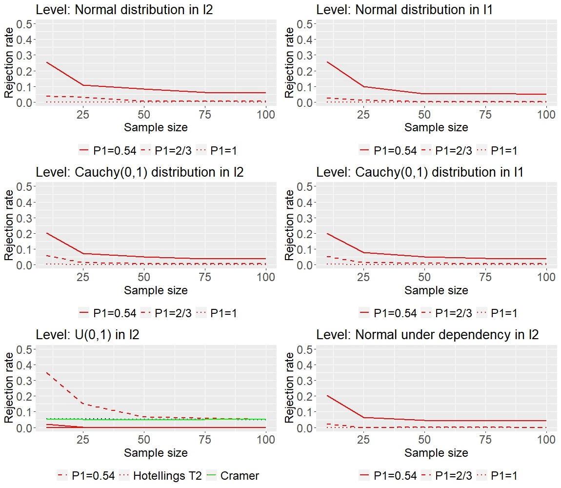
As expected, the averaged Wilcoxon test clearly outperforms in all scenarios. Further, in contrast to and , the averaged Wilcoxon tests are suitable for applications on high-dimensional data and show greater robustness to the deterioration of power with growing dimension. If not otherwise specified, the dimension of the data in the test problems is set to , samples are always balanced (i.e. ), the components of the data vectors are independent and the number of Monte Carlo iterations is . In the graphs in Figures 2-4, the full red line always represents the oracle test, the dashed red line represents , the dotted red line represents and the dashed blue line represents the independent Wilcoxon test.
4.2. Empirical level
In this section we investigate if the tests , and hold their nominal level, which was set to for all simulations presented in this section.
Independent Components. To study the empirical level of the tests , and we simulate i.i.d. data of a fixed dimension
where and and for two different scenarios: , , for the first scenario, , , for the second scenario. In both cases, the components of the vectors are independent and is either the or the distance. The results are shown in Figure 2 (upper and middle panels).
The level of the test is generally not upheld for sample sizes .
The effect of underestimation of the variance using the oracle value for is apparent, especially for very small sample sizes:
The effect is worse in the case of a normal distribution than in the Cauchy example. We note the difference in level in the normal example depending on the choice between and . We observe a drop between sample sizes and , a phenomenon which can be explained by a significant underestimation of variance using the asymptotic expansion (20) for small sample sizes.
Dependent Components. We developed the averaged Wilcoxon test inspired by the application to genomic microarray datasets, where common (parametric) assumptions are typically not met.
For instance, in the data example discussed in Section 5, it is unrealistic to assume that the components of the observed data vectors are independent. Our averaged Wilcoxon test does not pose any restrictive assumptions in this direction and is also applicable to dependent components. In this section, we therefore study the empirical level under dependence.
We consider as example for and
where denotes the 10-dimensional zero vector.
The oracle value in this example for dimension and Euclidean metric does not differ much from the independent case given in Table 6. We estimate for the oracle test.
The underestimation of the variance for smaller sample sizes can be observed in this example as well. The estimated levels are given in Figure 2. The performance is slightly better than in the independent case.
Uniform distribution. The last example we consider is given in dimensions for the uniform distribution, i.e.
where .
It is well known that parametric tests such as Hotelling’s may not perform well if the underlying parametric assumptions are violated. Indeed, Hotelling’s test does not uphold the nominal level in this example. The estimated levels of , , , and are given in Figure 2.
4.3. Power
In this section, we investigate the empirical power of all tests , , and in various scenarios.
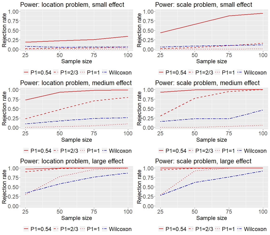
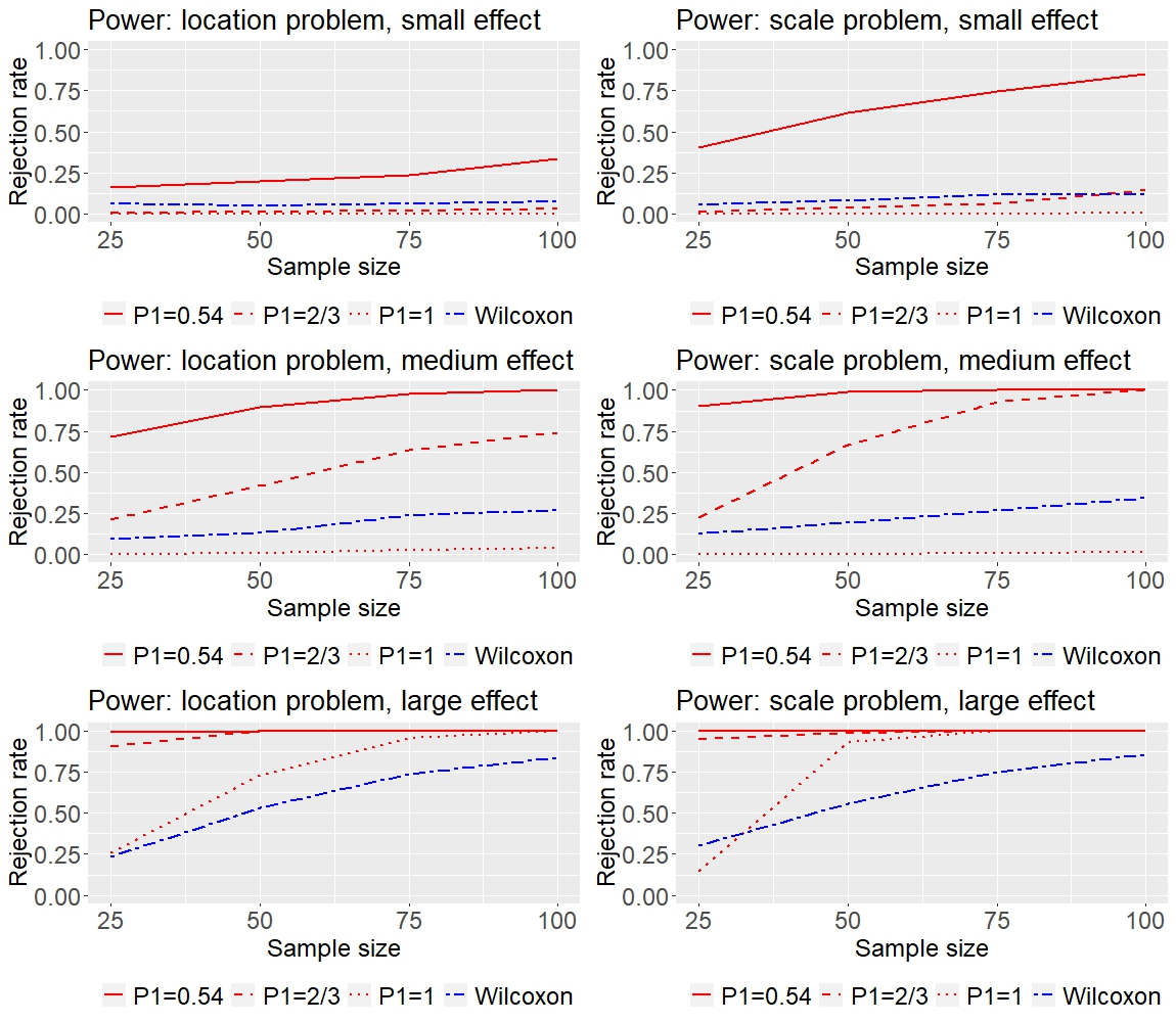
Power of , and in location and scale problems. We first consider simple Gaussian location and scale problems. The location and scale differences are present in all the dimensions, i.e. for the location problem, we generate data according to
| (28) |
where , . Here and in the following, we denote by and the -dimensional zero vector and identity matrix, respectively. For the scale problem, we consider
where . All tests have been performed for Manhattan () and Euclidean () distances, where the corresponding oracle values from Table 6 have been used. The results are shown in Figures 3-4. As expected, out of the three versions of the averaged Wilcoxon test, uniformly has the greatest power, while has the lowest. possesses non-trivial power in medium and large effect examples, while possesses non-trivial power in problems with large effect size only. We observe a slight loss of power of tests for the choice of metric over .

Deterioration of power in high dimensions. In this section, we consider problems in which a difference in location and scale is only present in one component for growing dimension . The sample sizes are between and . To be precise, we consider
and
where the covariance matrix is given by
| (29) |
i.e. the effect is limited to one dimension. In this and related problems, a deterioration of power occurs naturally as the dimensions grow, which is also confirmed by our simulation results. The tests are performed over the Euclidean metric since it has shown to outperform the Manhattan metric in Section 4.3. Figure 7 illustrates the loss of power due to increasing dimensionality for the two scenarios.
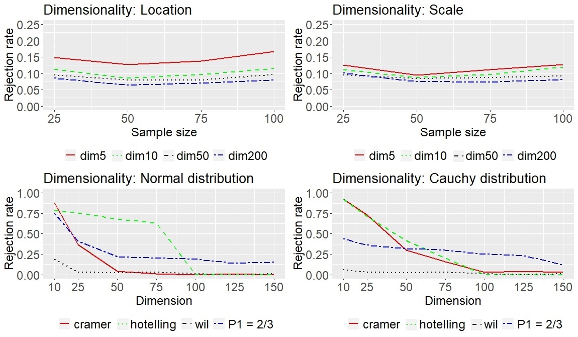
The deterioration of power due to the consideration of higher dimensions has been further examined and compared to other tests. The results of this set of simulations are presented in Figure 7, where greater stability of power over dimensions has been observed for the averaged Wilcoxon test. The test has been compared with Hotelling’s , Cramér’s and independent Wilcoxon tests, where the curves are denoted in blue, green, red and black, respectively. The tests have been compared in the location problem (28) and, additionally in a Cauchy location problem with
| (30) |
The sample size is fixed and the dimensions between and . The independent Wilcoxon test displays similar stability over dimensions to averaged Wilcoxon, albeit with significantly lower power. Although Cramér’s and Hotelling’s tests have higher power in problems of smaller dimension, these tests lose power rapidly and are less robust to dimensionality than the averaged Wilcoxon test.
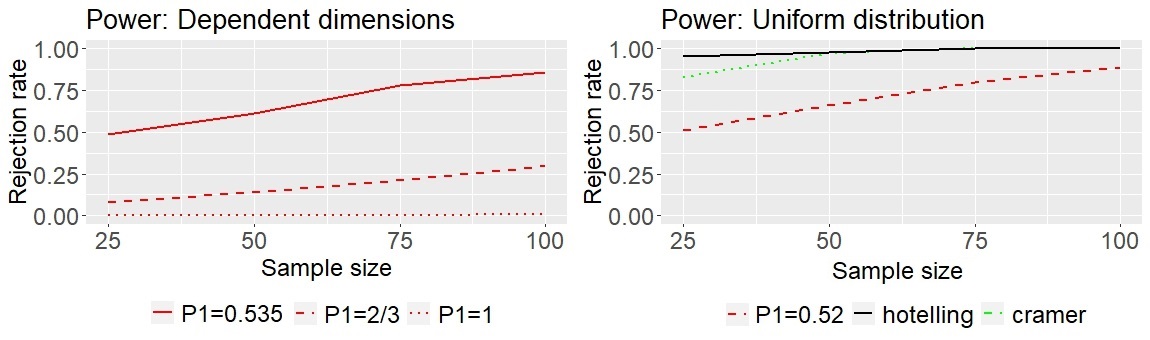
Dependence. We consider further the example given in 4.2 for the alternative
where , i.e. the normal location problem under dependence. The chosen oracle value is and the tests are performed with respect to the Euclidean distance. The results are given in Figure 5. We observe uniformly slight loss of power compared to the independent case.
Uniform example. For the uniform distribution considered in Section 4.2, we consider the alternative
and perform with respect to the Euclidean metric. The power of the test is compared to Hotelling’s and Cramér’s tests. The results are given in Figure 5.
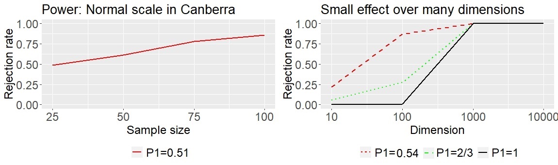
Power of the test for a non-standard distance. A potentially interesting distance function for the application to genomic microarray data is the Canberra distance, which proved to be well suited for distinguishing between groups of individuals based on their micro RNA profiles in hierarchical clustering algorithms (cf. Proksch et al., (2023)). Defined by , this quasi-normed distance equalizes the contribution of individual dimensions to the overall distance between points. Unfortunately, the Canberra distance is not a metric and in particular does not fulfill condition (D2) of Maa’s theorem. We therefore do not have a guarantee for the well-posedness of a test problem defined with respect to Canberra distances. The simulations also indicate that the location test over Canberra distance has almost no power in the examples considered here. However, it seems that it is possible to distinguish scale differences well, as illustrated in Figure 8. In this example, we test the scale difference of normal distributions with . Choosing and for the variance approximation grossly overestimates the variance due to the low oracle value (cf. Table 6). As a result, the corresponding test has low power. Nonetheless, the oracle value does have nontrivial power, further illustrating the necessity for a better variance approximation.
Lastly, Figure 8 visualises the examination of power of the three versions of the test for a small effect size over a large number of dimensions, i.e.
where with the dimension in the range from to . The graph is given in log scale. The convergence of power to as the dimension goes to infinity can be observed. However, for the example considered here, the and distance outperform the test based on pair-wise Canberra distances.
5. Real Data Example
Simulated examples indicate the stability of the power of averaged Wilcoxon tests with increasing dimension, making the test a viable choice for high-dimension low-sample-size problems (HDLSS). An example of such settings are genetic studies in which the goal is to detect the genes most differentially expressed between groups from diverse populations. Contrasting groups can give an indication of underlying mechanisms that cause the group differentiation, e.g. indicate gene-disease associations or genetic characteristics of groups. Genomic microarray datasets usually possess large number of features (dimensions, genes) while at the same time having low sample sizes, especially relative to their dimension. On the one hand, performing such measurements is still very costly and complex. On the other hand, one fundamental limitation causing this predicament is low population size, specifically, low number of people with a particular disease, property or a set of properties, relative to the number of observed variables, which emphasizes the relevance of methods tailored to HDLSS settings.
The following practical example is based on the dataset corresponding to the study T. et al., (2020) examining micro RNA (miRNA) levels in blood plasma of patients with lung adenocarcinoma. The dataset consists of raw counts of originally miRNAs (features in this example) in samples across groups. Groups are labeled ”granuloma”, ”cancer”, ”exosomes granuloma”, ”exosomes cancer”, ”without exosomes granuloma” and ”without exosomes cancer”. The study aims at differentiating between the patients with lung cancer and misdiagnosed patients with benign conditions. The samples of the cancer groups and the rest of the samples are, for the purposes of this example, pooled resulting in sample sizes (pooled cancer) and (pooled healthy). The measurements are represented in counts per million (CPM). CPM is a normalization method for RNA sequencing data that represents the number of reads of particular RNA scaled by the total number of reads in the sample, then multiplied by one million to facilitate comparisons between samples. Ad hoc dimensionality reduction has already been performed by including only the miRNAs which have counts per million larger than in more than sample, excluding the miRNAs that have low concentrations and are rarely measured (Anders et al., (2013), p24). Only the miRNA with CPM larger than have been included in the dataset.
| miRNA | log-fold change | log-CPM | p-value | BH correction |
|---|---|---|---|---|
| hsa-miR-3529-3p | 2.272515 | 9.817300 | 4.820727 | 7.274476 |
| hsa-miR-7-5p | 2.131011 | 9.013191 | 6.358140 | 4.797217 |
| hsa-miR-576-3p | 1.590984 | 9.030031 | 1.123073 | 5.649059 |
| hsa-miR-1827 | 1.673530 | 4.110844 | 2.038026 | 6.829125 |
| hsa-miR-4306 | 1.948530 | 8.998243 | 2.262798 | 6.829125 |
| hsa-miR-9-5p | 2.400299 | 7.625194 | 5.718436 | 1.351211 |
| hsa-miR-501-5p | 3.018604 | 4.190806 | 7.337386 | 1.351211 |
| hsa-miR-629-3p | 3.218628 | 3.371337 | 7.622035 | 1.351211 |
| hsa-miR-1180-3p | 1.384724 | 9.953922 | 9.180467 | 1.351211 |
| hsa-miR-92b-5p | 1.718041 | 6.529031 | 9.441425 | 1.351211 |
| hsa-miR-218-5p | 2.803250 | 7.846570 | 9.849784 | 1.351211 |
| hsa-miR-3158-3p | 1.702470 | 5.964335 | 1.371379 | 1.724509 |
| hsa-miR-181a-2-3p | 1.221580 | 8.373332 | 3.234169 | 3.754124 |
| hsa-miR-500a-5p | 5.036958 | 3.772247 | 4.843275 | 5.183284 |
| hsa-miR-877-5p | 1.638779 | 5.765388 | 5.152369 | 5.183284 |
It is important to note that the test results over pooled groups are not necessarily biologically meaningful. However, the example provided is self-consistent in the sense that the results of standard differential expression tools as used by bioinformaticians (e.g. exact tests over normalized counts with multiplicity correction, see Robinson et al., (2010))
have been confirmed by using averaged Wilcoxon-based tests. The example furthermore illustrates well the necessity of testing at least two out of three equalities of distance distributions from Maa’s theorem.
Differential expression analysis has been performed on the pooled dataset using the edgeR package in R. The in the package implemented procedure uses a locally exact test for differences in mean between two groups, which assumes a negative binomial distributions of miRNA counts and adjusts -values according to the Benjamini-Hochberg correction. The first most differentially expressed miRNAs are given in Table 1, reported with log-fold changes and log-CPM for completeness. The procedure makes discoveries based on adjusted -values below .
| Dimensions | p | p | ||
|---|---|---|---|---|
| 1.2 | 3.13356… | 0.00086 | -2.06327… | 0.01954 |
| 1.3 | 1.49720… | 0.06717 | -2.62111… | 0.00438 |
| 1.4 | 1.49987… | 0.06682 | -2.62000… | 0.00439 |
| 1.5 | 2.18150… | 0.01457 | -3.14900… | 0.00081 |
| 1.6 | 2.15037… | 0.01576 | -3.15471… | 0.00080 |
| 1.7 | 2.13957… | 0.01619 | -3.15738… | 0.00079 |
| 1.8 | 2.14050… | 0.01615 | -3.15757… | 0.00079 |
| 1.9 | 1.26487… | 0.10295 | -2.94173… | 0.00163 |
| 1.10 | 1.25779… | 0.10423 | -2.94330 … | 0.00162 |
These results are then compared with the test over the Euclidean distance for the test problems and , where represents the healthy group and the sick group. Note that the results of the tests are similar over other -induced metrics. The dimensions are added stepwise according to the list obtained by differential expression analysis in Table 1. The test of the first hypothesis detects the difference in distributions of , the distance between the points in the healthy group and , the distance between the points in sick and healthy groups, while the second compares the distances between the sick with . The test statistics and corresponding p-values are given in Table 2. The second test confirms the first discoveries, while the first test does not reject for the combinations of first , , and features.
6. Outlook
With this article, we introduced a Wilcoxon-inspired rank-based test for two-sample homogeneity test problems over interpoint distances, which provides a straightforward way for dimensionality reduction. The advantages of the test, which inherits some of its properties from the Wilcoxon test, include weak regularity conditions on the underlying distributions enabling comparisons for location, scale and shape problems, readily available critical values, and robustness against high-dimensionality. A procedure revolving around this test would include the choice of a metric or dissimilarity function between the points tailored to the structure of the data. We examined the power of the test in different situations and illustrated its use on microarray data, all of which underlines the potential of the proposed test. While, for simplicity of the argument, we concentrated on situations for which ties in distance comparisons do not occur, we believe that the results of this paper can be generalized to cases where ties are possible (discrete distributions and corresponding, suitably chosen metrics). A discrete version of Maa’s theorem provides a basis for such an approach. While the dependence structure in the case allowing for ties changes, the orders of the dependency neighbourhoods do not, as well as the orders of other relevant quantities in Theorem 6 needed to ensure a Gaussian limit. Naturally and notably, allowing for ties would necessitate a refined variance estimation for the implementation of the test.
We further illustrated the loss of power in low sample size situations due to the choice of an estimator for the probability in the variance approximation. The variance is, on one hand, underestimated by the use of oracle values for and, on the other hand, overestimated by the general upper bound provided by Theorem 3. The power of the test could further be increased in low sample size situations by improving the variance estimate, foremost by tightening the bound on , but also by including higher-order terms in the asymptotic expansion of the variance. The probability is an object interesting on its own merit. While the probability is a universal quantity over all underlying distributions and metric choices, depends on dimension, distribution and metric, as demonstrated by numerical simulations and indicated by two specific examples considered in this article.
We conjecture that a tighter upper bound, dependent on dimension and metric, can be established that clarifies the interplay of these parameters. However, this seems to be highly non-trivial and will be considered in future research.
On the other side, the universality of the lower bound on is not clear. By means of Theorem 6 we cannot guarantee the convergence of the test statistics for distributions for which (given that these exist). The characterization of is an interesting problem that we intend to study further.
Compared to some competitors computing the test statistic is computationally expensive.
This arises from the necessity of making all possible comparisons between induced distances, which, given balanced samples, results in a computational cost of order .
For comparison, note that the energy distance based test and Cramér test are of the order . Nonetheless, it is important to note that no further computations are necessary in order to apply the test since, when using the universal bound on the variance, the critical values are readily available and do not require expensive resampling approaches.
Despite the advocated use case for the test revolving around the low sample size setting, this inherent cost plays a significant role if the test is to be integrated into a multiple testing framework, as illustrated by the practical differential expression example.
Another interesting question warranting further investigation is the suitability of the distribution of non-standard and pseudo differences, such as the Canberra distance, which is of special interest in applications for the purpose of homogeneity testing. Namely, the theorem of Maa et al. does not guarantee the equivalence of testing for equal distributions over the Canberra distance function, since it does not fulfill the scalability and translational invariance property (D2). The arguments for the lower bound on given in the proof of Theorem 3 do not apply to the Canberra distance function, either. However, it has been indicated that the test based on the Canberra distance could be sensitive to scale problems. Under which additional conditions on the underlying distributions of and the theorem of Maa et al. remains valid should be considered as a question for future research.
Acknowledgements
Annika Betken gratefully acknowledges financial support from the Dutch Research Council (NWO) through VENI grant 212.164.
7. Appendix
7.1. Proof Theorem 1
corresponds up to a multiplicative constant to the second order -statistics with kernel of the degree . By the strong law of large numbers for multisample -statistics (e.g. Theorem 3.2.1, p.97 in Korolyuk and Borovskich, (2013)), we have the convergence.
7.2. Proof Theorem 2
Since, by assumption, ties in the distance comparisons considered here almost surely do not occur, the second sum in (9) is constant almost surely. Therefore, the test statistic and its variance correspond to (16) and (18), respectively, and we find
| (31) |
where and
. The asymptotic order of the first summand, which corresponds to the diagonal elements of the variance, is hence given by , i.e. for some constant . Note that by the assumption. In order to determine the (order of the) asymptotically leading term, we will now decompose the index set according to the amount of shared indices: . The most frequent occurrence is the case , i.e., most pairs share exactly one index. We define the set such that it contains exactly these indices and set . We find that the number of the pairs sharing two or more indices is of the order : we have order of choices for the two fixed indices and order choices for the rest of the indices. There are less pairs sharing three indices and therefore . and are hence of the same asymptotic order, namely of order : we have choices for fixing one index and order of choices for the rest of the indices. The asymptotically dominating part of the sum in (31) is therefore that over pairs which share exactly one index.
A pair of multiindices sharing exactly one index corresponds to a probability , e.g., for the case it is . Since under the null hypothesis with no ties
there are only two possible values of the probability if the multiindices share exactly one index (namely and ). Therefore, in the following we will rewrite the second term of the variance such that it only contains the terms and The final task in this proof is to count the occurrences of each.
Notice that we have by assumption, which guarantees that the summands in the second sum in (18) are positive, while are negative. In consequence there is a number of cancelling pairs in the sum. All the possible configurations of such such that with their probabilities expressed in terms of are given in Table 3. Note that Table 3 is symmetric both in the sense of the corresponding probabilities as well as regarding the number of instances in each case.
Counting the elements in the relevant index sets
In the following, we count the number of all pairs sharing exactly one index case by case.
Case 1: .
The first case is , i.e. we will determine the cardinality where
Let be fixed. There are possible choices for , where
| (32) |
(since ). There are choices for , since , , and are excluded, i.e. already chosen. There are possibilities for , since is excluded. We abbreviate for a fixed
For a fixed it is therefore
We obtain the desired cardinality by summation over all :
| (33) |
and since it is
we have
For the terms in (7.2), we find
as well as
and . Plugging these results into Eq. (7.2), we obtain
| (34) |
The final results of all other cases discussed below will be expressed as multiples of .
Case 2: results in .
Let . In this case, for any fixed , there are and possibilities to choose and , then and possible choices for and since and indices have already been chosen and fixed and there are and possibilities for and . It is therefore
Since
we conclude .
Case 3: results in .
Similarly, for we have, for a fixed , possibilities for the choice of , possibilities for the choice of since , and for and and and for and and therefore
Since the latter sum equals , we conclude .
Cases 4 and 5: and result in .
For a fixed there are choices for and , choices for where
and furthermore choices for choices for and choices for and therefore
where is the number of different possibilities to pick indices and between and such that . The same for the ordering . This yields
and hence . Since it holds , we also obtain .
Case 6: results in .
Let be fixed. Choosing a element subset of the rest of points defines and , i.e. there are possibilities and similarly, there are possibilities to chose and from the rest of points, while and can be chosen in and ways, therefore having
and we conclude .
Case 7: results in .
For fixed , there are choices of and and choices for and , and for and therefore having
Combining the findings of Case 1 - Case 7
For the rest of the cases in Table 3 the combinatorial symmetry holds. We therefore have , , and , as summarized in Table 5 below, where all cardinalities are listed as multiples of the reference cardinality .
| 1 | ||||
Since the corresponding summands in the sum (31) are negative and we conclude
By (31) and the negligibility of the diagonal elements and of the sums over pairs sharing and indices, the claim of the theorem follows.
7.3. Proof Theorem 3
We first prove that . to this end, let where and share exactly the first two indices, i.e.
We now show that and that .
Since , …, are i.i.d., so are the random variables , and . We rewrite as
It is therefore
having . If , i.e. ties almost surely do not occur, is one of equally probable orderings of three distances and we conclude
for any underlying distribution.
Recall the definition of under null hypothesis:
Denoting by we similarly have
where , , and are identically distributed but and stochastically dependent. Since any permutation of the tupel swapping and or and retains its distribution (e.g. ), we have
| (35) |
and
| (36) |
By decompositions
and
we have
Since we conclude that and therefore
again, for any underlying distribution of , which establishes the second inequality of (22).
It remains to show the first inequality in (22). Let the first condition of the theorem hold, i.e. let the support of the density of the distribution be unbounded, with for any , and let , where , and be three independent instances of . By Example 1 it is then
Let further be such that . By the triangle and reversed triangle inequalities it is
and we conclude that if . Since is monotonically decreasing with global minimum at , for such it is
and therefore
Since we conclude that .
Otherwise, let the second condition hold, i.e. let the distribution of be such that (2) holds. Note that iff almost surely. We have
for some and all , where the inequality is strict on a set with positive mass and therefore
For the continuous function this is a contradiction to a.s. Hence we conclude .
7.4. Central limit theorem for locally dependent variables
For the sake of completeness, in the following we formulate the used version of CLT for triangular arrays under local dependency (represented by a dependency graph) as developed in Liu and Austern, (2023). Suppose that is a real number and . is defined as an infinite index set and the accompanying sequence of finite subsets with with . For a triangular array of the form we define
where . The triangular array induces the dependency graph with
The necessary condition on the dependence structure holding for all is defined as the following condition:
[LD*] There exist the dependency graph s.t. for all disjoint subsets if there are no edges between and , then is independent of .
The set of vertices in the neighborhood of is defined as
We can proceed to formulate the statement corresponding to the Theorem 3.3 in (Liu and Austern, (2023)).
Theorem 6.
Suppose that is a triangular array of mean zero random variables satisfying [LD*], and that the cardinality of index set is upper-bounded by for any . Furthermore, assume that
| (37) |
Then there is such that for all we have
for some constant that only depends on .
7.5. Proof of Theorem 4
Theorem 4 is proved by an application of Theorem 6. Accordingly, we have to show that Asssumption [LD*] holds and that (37) is satisfied. To verify Asssumption [LD*], note that and , defined by the relation if and only if and ,
induce an undirected loopless graph .
Moreover, for , since by assumption is monotonically increasing in .
For two disjoint subsets , no edges between and means that for any two indices entering and entering it holds that . As a result, and are composed of functions of disjoint subsets of . Since the latter set consists of mutually independent random variables, the set is independent of .
Therefore, for the graph defined in the above manner,
condition [LD*] of Theorem 6 holds.
For showing that condition (37) of Theorem 6 is fulfilled, recall that the statistic we are interested in is defined as follows:
| (38) |
with for , , and . We show that condition (37) is fulfilled for the above statistic when . For this, we first determine a lower bound for . Note that
The sum on the right-hand side of the above equation is asymptotically dominated by summands for which and share exactly one index. The rest of the summands, i.e. those where and share two, three, or four indices are asymptotically of lower order (cf. proof of Theorem 2), such that
By definition of and
Our goal is to determine the above expression explicitly. For this, we express in terms of the following quantities:
for which, due to the fact that ,
As in the proof of Theorem 2, to determine we make a case distinction with respect to which elements of and coincide.
The argument for the individual cases is analogous to the proof of Lemma 2.l
Case 1:
Note that
where and , i.e. and are independent, identically distributed random variables with . It follows that . Therefore, we have
Case 2: , Case 3: , Case 4:
Due to symmetry of and interchangeability of and , the same argument as in Case 1
yields .
Case 5:
Note that
where and , i.e. and are independent random variables with and . It follows that . Therefore, we have
Case 6: , Case 7: , Case 8:
Due to symmetry of and interchangeability of and , the same argument as in Case 5 yields .
Case 9:
Note that
where and , i.e. and are independent, identically distributed random variables with . It follows that . Therefore, we have
Case 10:
Note that
where and , i.e. and are independent, identically distributed random variables with . It follows that . Therefore, we have
The number of summands of each case contributing to the variance reported in (38) can be determined analogously as in the proof of Theorem 2. Table 5 represents all the possible configurations of and sharing exactly one index and the corresponding number of summands as multiplicities of the number of summands corresponding to Case 1 (), i.e. , where
| 1 | ||||
It follows that
since and . Since by assumption, it holds that
for some positive constant .
Noting that and , we conclude
| (39) |
The right-hand side of the above inequality is positive if . For it suffices that is not almost surely constant. Overall, it follows that
| (40) |
where is a positive constant that does not depend on or .
In order to verify condition (37) of Theorem 6
we have to establish an upper-bound on the cardinality of dependency neighbourhoods for any two vertices , of the graph .
We have
| (41) |
where
denotes the number of elements of any dependency neighbourhood of order one, since due to definition of the edge set all vertices possess the same number of adjacent vertices (c.f. Combinatorial Quantities 7.7).
Combining (40) and (41), for proving validity of (37) we conclude that
where is a constant not depending on the sample sizes and . By (42) and (43) in Section 7.7, we have
i.e. and . By (34) in Section 7.1, it holds that
i.e. and hence, for and large enough and some constant we have
Since as ,
condition (37) of Theorem 6 is fulfilled for . As a result, the distribution of converges to a normal distribution in Wasserstein-1 distance with convergence rate .
7.6. Proof of Theorem 5
Under a fixed alternative for which it holds , due to Theorem 1 we have
The order of , variance of under null hypothesis, is the same as the order of (cf. proof of Theorem 4) and there exists some constant s.t.
On the other hand, with and
with a positive constant and for the -Level critical value hence
7.7. Combinatorial Quantities
In this subsection we count the quantities corresponding to the index sets and the local dependency structure of the triangular arrays in Section 2, i.e. find the order of , the degree of a vertex , necessary for the estimations figuring in Theorem 6. These quantities only depend on the sizes of two groups and , where we assume that is large enough to perform the independent sampling described in Section 2. For the sake of completeness, we also calculate the combinatorial constants in (9) and the sizes of the related sets.
We firstly count the number of elements in the index sets and . is the number of ways we can pick two points from the point cloud and we combine this choice with ways we can combine one of the remaining -points with one of the -points, having
| (42) |
Similarly, in order to choose two between-clouds distances, we can pick two points from and two points from in and and we can connect them in two ways, concluding
For it is therefore
We further estimate the size of the dependency neighborhoods (degree of the vertices) of and in the dependency graph generated by the triangular array defined in (11). We notice that all the vertices of a type ( or ) have the same degree. In both cases, two vertices and are connected iff and multiincides and can share up to elements. The highest number of vertices connected to shares only one element of and the number of connections with a larger intersection is of lesser order than this number.
We count for . Firstly we count the number of elements in the complementary set, i.e. for the fixed we count the number of from independent vertices in and in . In the first case, there are possibilities to pick by excluding indices in . For it is then
| (43) |
We further consider . There are possibilities to pick with . Then since it is we calculate
Similarly, regarding for , we consider the complementary set, the set of all with . In the case we have and in the case we have possibilities. We conclude that the cardinality of the dependency neighbourhood of is
| (44) |
We can determine the cardinality of by combining all the choices of pairwise connected points from the first group with all the choices of connections between the rest points of the first group with points of the second, where . We therefore have
| (45) |
where . This can be further simplified as .
We proceed to calculate the number of elements in as
By fixing a pair of tupels (i.e. by fixing some four vertices , , and ), we analogously have
The constant simplifies to
| (46) |
Similarly, by fixing two pairs , , , , we have
which reduces the constant to
| (47) |
7.8. Numerical estimation of over distributions, metrics and dimensions
The probability (13) has been estimated by Monte Carlo samplings for concrete distributions, metrics and dimensions as given in Tables 6-9. The exemplified distributions include standard normal, uniform, Gamma with shape parameter and scale parameter and Cauchy distribution with location and scale . Particularly the heavy-tailed distributions were of interest, since the concentration of the distribution determines . The dimensions are always independent. Note that the estimated values hold true for any scaling or translation of the examined distributions, given the independence of the dimensions, due to (D1), except for the Canberra distance. Canberra refers to Canberra distance function given with , which is of special interest.
| Metric\Dimension | 1 | 2 | 5 | 10 | 50 |
|---|---|---|---|---|---|
| 0.528276 | 0.532446 | 0.534103 | 0.534561 | 0.534962 | |
| 0.528205 | 0.533552 | 0.536747 | 0.538320 | 0.533520 | |
| 0.527722 | 0.533157 | 0.535111 | 0.533912 | 0.530244 | |
| 0.527916 | 0.531780 | 0.531696 | 0.528262 | 0.517773 | |
| Canberra | 0.532763 | 0.506087 | 0.505927 | 0.506346 | 0.506765 |
| Metric\Dimension | 1 | 2 | 5 | 10 | 50 |
|---|---|---|---|---|---|
| 0.510712 | 0.514656 | 0.514466 | 0.515283 | 0.516251 | |
| 0.511553 | 0.517824 | 0.521306 | 0.522040 | 0.522902 | |
| 0.510950 | 0.519395 | 0.523481 | 0.524618 | 0.524708 | |
| 0.510413 | 0.518092 | 0.521787 | 0.518908 | 0.510352 | |
| Canberra | 0.536694 | 0.540395 | 0.540820 | 0.541016 | 0.541079 |
| Metric\Dimension | 1 | 2 | 5 | 10 | 50 |
|---|---|---|---|---|---|
| 0.536443 | 0.544270 | 0.549540 | 0.551535 | 0.552521 | |
| 0.535988 | 0.545402 | 0.553075 | 0.557083 | 0.562266 | |
| 0.536178 | 0.544418 | 0.551290 | 0.555977 | 0.561372 | |
| 0.536259 | 0.544070 | 0.550366 | 0.552803 | 0.555821 | |
| Canberra | 0.532183 | 0.531522 | 0.530954 | 0.530633 | 0.530991 |
| Metric\Dimension | 1 | 2 | 5 | 10 | 50 |
|---|---|---|---|---|---|
| 0.556312 | 0.564395 | 0.570460 | 0.573040 | 0.576032 | |
| 0.557003 | 0.564242 | 0.569137 | 0.571805 | 0.572302 | |
| 0.555691 | 0.563025 | 0.568439 | 0.570655 | 0.570892 | |
| 0.556125 | 0.564030 | 0.567522 | 0.569805 | 0.571181 | |
| Canberra | 0.532626 | 0.507481 | 0.508951 | 0.508473 | 0.506963 |
| Metric\Dimension | 1 | 2 | 5 | 10 | 50 |
|---|---|---|---|---|---|
| 0.556344 | 0.563713 | 0.568862 | 0.571261 | 0.574518 | |
| 0.556311 | 0.562560 | 0.568479 | 0.570540 | 0.573249 | |
| 0.554668 | 0.562374 | 0.567011 | 0.568981 | 0.570871 | |
| 0.557274 | 0.561351 | 0.568047 | 0.568846 | 0.570900 | |
| Canberra | 0.536604 | 0.540105 | 0.540209 | 0.540613 | 0.542141 |
References
- Anders et al., (2013) Anders, S., McCarthy, D. J., Chen, Y., Okoniewski, M., Smyth, G. K., Huber, W., and Robinson, M. D. (2013). Count-based differential expression analysis of rna sequencing data using r and bioconductor. Nature protocols, 8(9):1765–1786.
- Anderson, (2003) Anderson, T. W. (2003). An introduction to multivariate statistical analysis. Third Edition., volume 2. Wiley New York.
- Baringhaus and Franz, (2004) Baringhaus, L. and Franz, C. (2004). On a new multivariate two-sample test. Journal of multivariate analysis, 88(1):190–206.
- Betken, (2016) Betken, A. (2016). Testing for change-points in long-range dependent time series by means of a self-normalized Wilcoxon test. Journal of Time Series Analysis, 37(6):785–809.
- Brécheteau, (2019) Brécheteau, C. (2019). A statistical test of isomorphism between metric-measure spaces using the distance-to-a-measure signature. Electronic Journal of Statistics, 13(1):795–849.
- Chazal et al., (2011) Chazal, F., Cohen-Steiner, D., and Mérigot, Q. (2011). Geometric inference for probability measures. Foundations of Computational Mathematics, 11:733–751.
- Chenouri and Small, (2012) Chenouri, S. and Small, C. G. (2012). A nonparametric multivariate multisample test based on data depth. Electronic Journal of Statistics, 6(none):760 – 782.
- Chernozhukov et al., (2017) Chernozhukov, V., Galichon, A., Hallin, M., and Henry, M. (2017). Monge–Kantorovich depth, quantiles, ranks and signs.
- Weitkamp et al., (2024) Weitkamp, C. A., Proksch, K., Tameling, C. and Munk, A. (2024). Distribution of distances based object matching: Asymptotic inference. Journal of the American Statistical Association, 119(545):538–551.
- Datta and Satten, (2005) Datta, S. and Satten, G. A. (2005). Rank-sum tests for clustered data. Journal of the American Statistical Association, 100(471):908–915.
- Deb and Sen, (2023) Deb, N. and Sen, B. (2023). Multivariate rank-based distribution-free nonparametric testing using measure transportation. Journal of the American Statistical Association, 118(541):192–207.
- Dehling et al., (2013) Dehling, H., Rooch, A., and Taqqu, M. S. (2013). Non-parametric change-point tests for long-range dependent data. Scandinavian Journal of Statistics, 40(1):153–173.
- Dehling et al., (2017) Dehling, H., Rooch, A., and Taqqu, M. S. (2017). Non-parametric change-point tests for long-range dependent data. Electronic Journal of Statistics, pages 2168 – 2198.
- Franz and Franz, (2019) Franz, C. and Franz, M. C. (2019). Package ‘cramer’.
- Geenens et al., (2023) Geenens, G., Nieto-Reyes, A., and Francisci, G. (2023). Statistical depth in abstract metric spaces. Statistics and Computing, 33(2):46.
- Gellert et al., (2019) Gellert, M., Hossain, M. F., Berens, F. J. F., Bruhn, L. W., Urbainsky, C., Liebscher, V., and Lillig, C. H. (2019). Substrate specificity of thioredoxins and glutaredoxins–towards a functional classification. Heliyon, 5(12):e02943.
- Gerstenberger, (2021) Gerstenberger, C. (2021). Robust discrimination between long-range dependence and a change in mean. Journal of Time Series Analysis, 42(1):34–62.
- Gijbels and Nagy, (2017) Gijbels, I. and Nagy, S. (2017). On a General Definition of Depth for Functional Data. Statistical science, 32(4):630–639.
- Gnettner et al., (2023) Gnettner, F., Kirch, C., and Nieto-Reyes, A. (2023). Variations of the depth based Liu-Singh two-sample test including functional spaces. arXiv preprint arXiv:2308.09869.
- Gombay and Huskova, (1998) Gombay, E. and Huskova, M. (1998). Rank based estimators of the change-point. Journal of statistical planning and inference, 67(1):137–154.
- Gretton et al., (2006) Gretton, A., Borgwardt, K., Rasch, M., Schölkopf, B., and Smola, A. (2006). A kernel method for the two-sample-problem. Advances in neural information processing systems, 19.
- Hallin et al., (2021) Hallin, M., Del Barrio, E., Cuesta-Albertos, J., and Matrán, C. (2021). Distribution and quantile functions, ranks and signs in dimension d: A measure transportation approach.
- Henze, (1988) Henze, N. (1988). A multivariate two-sample test based on the number of nearest neighbor type coincidences. The Annals of Statistics, 16(2):772–783.
- Hoffman et al., (2001) Hoffman, E. B., Sen, P. K., and Weinberg, C. R. (2001). Within‐cluster resampling. Biometrika, 88(4):1121–1134.
- Korolyuk and Borovskich, (2013) Korolyuk, V. S. and Borovskich, Y. V. (2013). Theory of U-statistics, volume 273. Springer Science & Business Media.
- Liu et al., (2022) Liu, J., Ma, S., Xu, W., and Zhu, L. (2022). A generalized Wilcoxon–Mann–Whitney type test for multivariate data through pairwise distance. Journal of Multivariate Analysis, 190:104946.
- Liu, (1990) Liu, R. Y. (1990). On a Notion of Data Depth Based on Random Simplices. The Annals of Statistics, 18(1):405 – 414.
- Liu and Singh, (1993) Liu, R. Y. and Singh, K. (1993). A Quality Index Based on Data Depth and Multivariate Rank Tests. Journal of the American Statistical Association, 88(421):252–260.
- Liu and Austern, (2023) Liu, T. and Austern, M. (2023). Wasserstein-p bounds in the central limit theorem under local dependence. Electronic Journal of Probability, 28:1–47.
- Maa et al., (1996) Maa, J.-F., Pearl, D. K., and Bartoszyński, R. (1996). Reducing multidimensional two-sample data to one-dimensional interpoint comparisons. The Annals of Statistics, 24(3):1069 – 1074.
- Mahalanobis, (2018) Mahalanobis, P. C. (2018). On the generalized distance in statistics. Sankhyā: The Indian Journal of Statistics, Series A (2008-), 80:pp. S1–S7.
- Montero-Manso and Vilar, (2019) Montero-Manso, P. and Vilar, J. A. (2019). Two-sample homogeneity testing: A procedure based on comparing distributions of interpoint distances. Statistical Analysis and Data Mining: The ASA Data Science Journal, 12(3):234–252.
- Möttönen and Oja, (1995) Möttönen, J. and Oja, H. (1995). Multivariate spatial sign and rank methods. Journal of Nonparametric Statistics, 5(2):201–213.
- Oja, (1983) Oja, H. (1983). Descriptive statistics for multivariate distributions. Statistics & Probability Letters, 1(6):327–332.
- Oja, (1999) Oja, H. (1999). Affine Invariant Multivariate Sign and Rank Tests and Corresponding Estimates: a Review. Scandinavian Journal of Statistics, 26(3):319–343.
- Proksch et al., (2023) Proksch, K., Di Bucchianico, A., Keizer, S., de Jongh, M., Regis, M., Rocchetta, R., Hang, C., Gomaz, L., Marjanovic, A., Nesenberend, D., et al. (2023). Personalised Health Monitoring for Early Disease Detection.
- Robinson et al., (2010) Robinson, M. D., McCarthy, D. J., and Smyth, G. K. (2010). edgeR: a Bioconductor package for differential expression analysis of digital gene expression data. bioinformatics, 26(1):139–140.
- Ross, (2011) Ross, N. (2011). Fundamentals of Stein’s method. Probability Surveys, 8(none):210 – 293.
- Shi et al., (2023) Shi, X., Zhang, Y., and Fu, Y. (2023). Two-Sample Tests Based on Data Depth. Entropy, 25(2).
- Székely et al., (2004) Székely, G. J., Rizzo, M. L., et al. (2004). Testing for equal distributions in high dimension. InterStat, 5(16.10):1249–1272.
- T. et al., (2020) T., K., X., W., Y., H., and K., W. (2020). TTF1 and TKTL1 mRNAs in extracellular vesicles as a blood biomarker for lung adenocarcinoma. Available at: https://www.ncbi.xyz/geo/query/acc.cgi?acc=GSE71661.
- Tukey, (1975) Tukey, J. W. (1975). Mathematics and the picturing of data. In Proceedings of the International Congress of Mathematicians, Vancouver, 1975, volume 2, pages 523–531.