SparseGrow: Addressing Growth-Induced Forgetting in Task-Agnostic Continual Learning

Abstract

In continual learning (CL), model growth enhances adaptability over new data, improving knowledge retention for more tasks. However, improper model growth can lead to severe degradation of previously learned knowledge, an issue we name as growth-induced forgetting (GIFt), especially in task-agnostic CL using entire grown model for inference. Existing works, despite adopting model growth and random initialization for better adaptability, often fail to recognize the presence of GIFt caused by improper model growth. This oversight limits comprehensive control of forgetting and hinders full utilization of model growth. We are the first in CL to identify this issue, and conduct an in-depth study on root cause of GIFt, where layer expansion stands out among model growth strategies, widening layers without affecting model functionality. Nonetheless, direct adoption of layer expansion presents challenges. It lacks data-driven control and initialization of expanded parameters to balance adaptability and knowledge retention. In this paper, we propose a novel sparse model growth (SparseGrow) approach to overcome the issue of GIFt while enhancing adaptability over new data. SparseGrow employs data-driven sparse layer expansion to control efficient parameter usage during model growth, reducing GIFt from excessive growth and functionality changes. It also combines the sparse growth with on-data initialization at training late-stage to create partially zero-valued expansions that fit learned distribution, enhancing retention and adaptability. To further minimize forgetting, freezing is applied by calculating the sparse mask, allowing data-driven preservation of important parameters. Through experiments across datasets with various task-agnostic settings, use cases and large number of tasks, we demonstrate the necessity of layer expansion and showcase the effectiveness of SparseGrow in overcoming GIFt, highlighting its adaptability and knowledge retention for incremental tasks. Code will be available upon publication.

Introduction

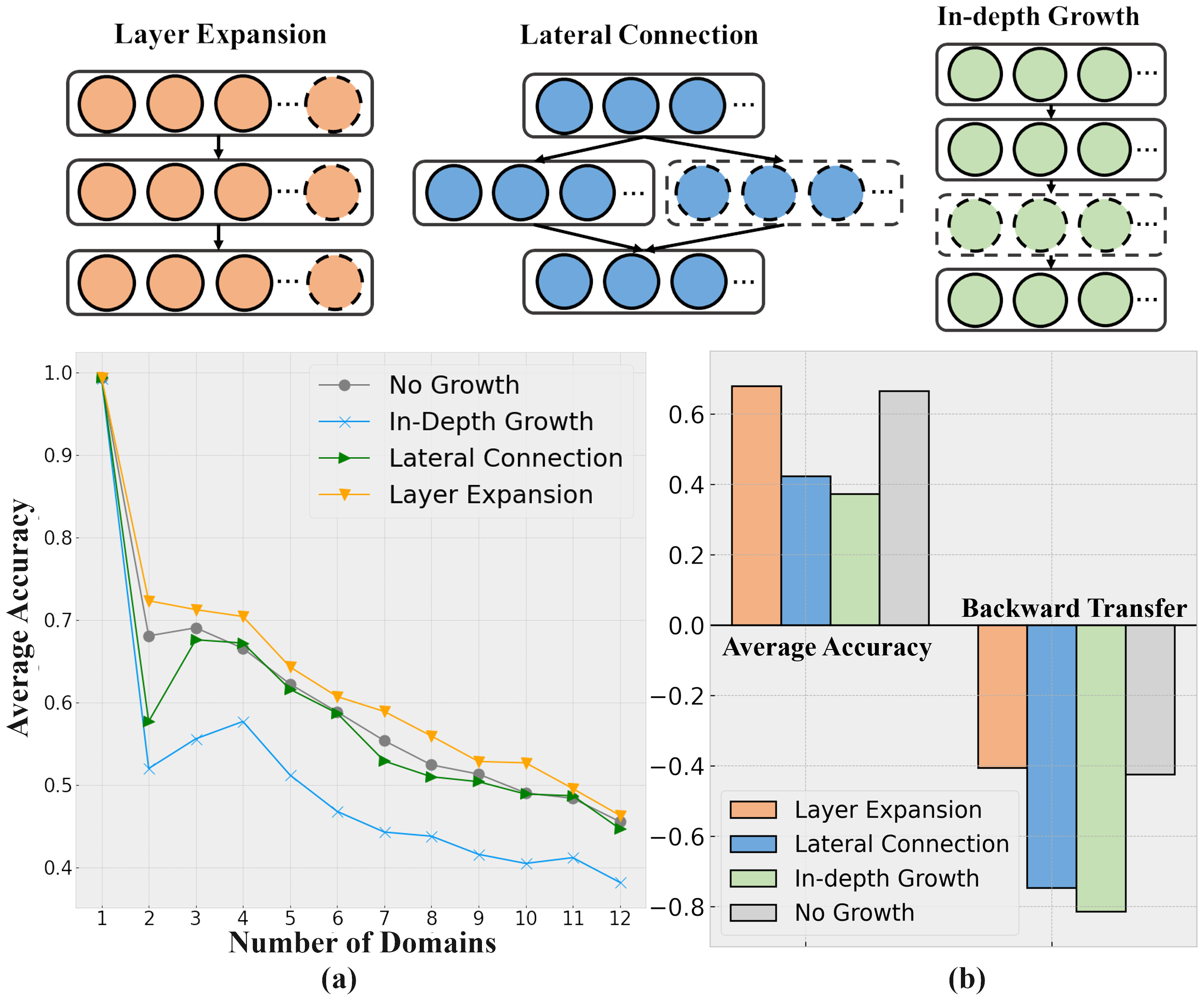
Figure 1: Comparison of three model growth methods applied to ResNet in handling sequential domains, contrasting with No Growth: 1) Layer Expansion widens each layer; 2) Lateral Connection adds lateral layers connected to adjacent layers, and 3) In-Depth Growth adds hidden layers to increase depth. (a) Shows the average accuracy change with these growth methods. (b) Displays their average accuracy and backward knowledge transfer. Layer Expansion excels in both, demonstrating better adaptability with less forgetting, even outperforming No Growth. Best viewed in color.

In the field of continual learning (CL), model growth becomes essential for better adaptation to new data, improving scalability in managing incremental data. In real-life scenarios with dynamic environments or evolving needs such as autonomous vehicles, healthcare and smart cities, model growth is crucial for model deployment in handling increased task complexity, incorporating new features or new modality data. As the volume of incremental data exceeds the model’s learning capacity, it struggles to adapt to new inputs or retain previous knowledge. This necessitates augmenting the model’s parameter capacity to sustain or enhance its adaptability, thereby improving scalability.

However, improper model growth often leads to a degradation of performance on previously learned tasks, an issue we identify and name as growth-induced forgetting (GIFt), especially in task-agnostic CL settings such as domain and class incremental learning settings (Shim et al. 2021; Hu et al. 2021). In these scenarios, the task label is unavailable, and the entire model, including expanded parameters, is used for inference. Differing from catastrophic forgetting (CF), which arises from data distribution changes, growth-induced forgetting is a distinct type of forgetting that occurs when a trained single model, upon increasing its parameter capacity through model growth, is affected in its ability to retain or effectively utilize previously learned information. This concept is echoed in neuroscience, where increasing neurogenesis in the brain after memory formation can promote forgetting, referred to as neurogenesis-based forgetting (Davis and Zhong 2017).

Some existing works in continual learning adopt different model growth strategies and randomly initialize them to enhance adaptability. However, they fail to recognize the presence of GIFt resulting from improper model growth. These methods may either be task-specific, requiring manual task identification during inference to avoid forgetting issues, not applicable for domain or class incremental scenarios, or adopting improper model growth strategies that may further lead to GIFt. Nevertheless, the lack of explicit acknowledgement of the growth-induced forgetting issue poses challenges in identifying suitable model growth approaches. This not only limits comprehensive control of forgetting but also hinders full utilization of model growth.

We are the first in CL to identify this issue and conduct an in-depth study to identify appropriate model growth strategies for increasing model capacity while minimizing the occurrence of growth-induced forgetting. Our research revealed that layer expansion, which widens layers without affecting model functionality, stands out compared with other model growth strategies, such as lateral connection and in-depth growth. The impacts of these growth methods on growth-induced forgetting (GIFt) differ: Layer expansion expands parameters in width, which are computed collectively during inference. Lateral connections add new modules in width connecting adjacent layers, overwriting old module values. In-depth growth adds new hidden layers, introducing new computations for preceding and succeeding parameters. Drawing inspiration from neurogenesis (Davis and Zhong 2017; Deng, Aimone, and Gage 2010), we propose a novel sparse model growth (SparseGrow) approach to overcome the issue of GIFt while enhancing adaptability. SparseGrow employs data-driven sparse layer expansion to control efficient parameter usage during model growth, reducing growth-induced forgetting caused by excessive growth and functionality changes. While achieving data-driven control, the choice of initialization values significantly impacts expansion, with zero-initialization stopping its update and random-initialization causing heavy GIFt. SparseGrow combines the sparse growth with on-data initialization at final stage of training to create partially zero-valued expansions that fit the learned distribution, minimizing GIFt while enhancing adaptability. To further minimize forgetting, freezing is applied by calculating the sparse mask, allowing data-driven preservation of important parameters. To validate our findings, we conducted comprehensive experiments on various task-agnostic settings with domain and class incremental datasets and varying numbers of tasks. The results demonstrate the necessity of layer expansion, showcasing the effectiveness of our approach in overcoming GIFt while highlighting the adaptability and knowledge retention of the method for incremental tasks.

Figure 2: SparseGrow training process overview. Due to high complexity or dissimilarity of new dataset (blue), model capacity limits its performance. Hence, there is a need to expand the model to enhance its adaptability and to reserve space for future data. Sparse training with freezing is throughout the training process. Sparsity level and freeze mask updates as model expands.

RELATED WORK

Growing Approaches

There are three principal model growth methods: 1) Layer Expansion (LayerExp), which grows in width by widening each layer of the model; 2) Lateral Connection (LatConn), which also grows in width by introducing new lateral layers connected to adjacent layers; and 3) In-depth growth (IDGrow) that adds hidden layers to increase model depth.

Lateral Connection

PNNs (Rusu et al. 2016) statically grow the architecture with randomly initialized modules while retaining lateral connections to previously frozen modules, limited to specific simple networks. (Schwarz et al. 2018) use randomly initialized active lateral columns to learn new tasks by connecting them to lateral columns that store previous knowledge, applicable to Conv2d layers. (Zhang et al. 2020) adopts AutoML-based model growing with both lateral connections and in-depth growth. VariGrow (Ardywibowo et al. 2022) proposes a task-agnostic CL approach that detects new tasks through an energy-based novelty score and grows a new expert module to handle them. (Hu et al. 2023) add a new branch called the task $t$ expert while freezing existing experts, introducing dense connections between the intermediate layers of the task expert networks. (Li et al. 2019) proposes a hybrid solution involving operations: ’new’, ’adaptation’, and ’reuse’, applicable to specially designed Conv2d networks. These methods demonstrate the potential of lateral connections for CL but highlight the need for more general approaches with less GIFt applicable for complex networks.

Layer Expansion

DEN (Yoon et al. 2017) uses layer expansion in a top-down manner, growing every layer if the loss does not meet a threshold. (Hung et al. 2019) expands the number of filters (weights) for new tasks and adopts gradual pruning to compact the model, limited to task-specific settings. (Ostapenko et al. 2019) expands the same number of neurons used in a layer in the GAN generator for rehearsal scalability. (Geng et al. 2021) expands the hidden size by the pruning ratio of task. (Yang et al. 2021) grow a randomly initialized expanded filter and concatenate it into the network. (Xu and Zhu 2018) adaptively expands each layer of the network when new task arrives, applicable for simple convolutional networks and fully-connected networks. (Yan, Xie, and He 2021) expand the model with new parameters by creating a separate feature extractor for incoming data, applicable for class-incremental learning. Our work could further exploit layer expansion’s potential by reducing GIFt.

In-Depth Growth

Kozal et al. (Kozal and Wozniak 2023) add new layers atop existing ones. Zhang et al. (Zhang et al. 2020) use AutoML for width and depth growth, incorporating lateral and in-depth layers with knowledge distillation. However, deepening the model tends to change the model architecture, is not general enough for complex models, and often affects knowledge retention.

Overcoming Growth-Induced Forgetting

The issue of growth-induced forgetting might have been indirectly addressed in the context of task-agnostic continual learning, where certain studies have focused on preserving knowledge post model growth. In task-agnostic CL, (Madaan et al. 2023) propose Quick Deep Inversion to recover prior task visual features and enhance distillation. (Ostapenko et al. 2019) expand the same number of neurons used in a layer in the GAN generator for the scalability of rehearsal. (Yan, Xie, and He 2021) freeze the previously learned representation and augment it with additional feature dimensions from a new learnable feature extractor. VariGrow (Ardywibowo et al. 2022) detects new tasks and grows a new expert module to handle them. By identifying GIFt, our work aims to address this issue at its root level, offering new strategies for enhancing knowledge retention.

Problem Formulation

We aim to enhance model adaptation to new data by expanding model capacity while addressing growth-induced forgetting in task-agnostic scenarios, covering domain-incremental and class-incremental learning. Given a sequence of non-iid datasets $\{\mathcal{D}_{1},\mathcal{D}_{2},\ldots,\mathcal{D}_{t}\}$ and a model $f(\cdot;\theta_{t})$ trained on previous datasets, where $\theta_{t}$ are the model parameters at time $t$. Accessing only the current dataset $\mathcal{D}_{t}$ at time $t$, the goal is to grow the model capacity to improve accuracy on $\mathcal{D}_{t}$ and future datasets while minimizing performance degradation on previous datasets. This is formalized as:

$$\text{minimize }J(\theta_{t})=\mathcal{L}(\mathcal{D}_{t};f(\cdot;\theta_{t}))+\lambda\sum_{i=1}^{t-1}\mathcal{L}(\mathcal{D}_{i};f(\cdot;\theta_{i}))$$

where $J(\theta_{t})$ is the objective function at time $t$, $\mathcal{L}(\cdot)$ is the loss function, $\lambda$ is a regularization parameter, $\mathcal{L}(\mathcal{D}_{t};f(\cdot;\theta_{t}))$ is the loss on the current dataset, and $\sum_{i=1}^{t-1}\mathcal{L}(\mathcal{D}_{i};f(\cdot;\theta_{i}))$ is the cumulative loss on previous datasets.

Methodology

Sparse Neural Expansion

Sparse neural expansion consists of layer expansion and dynamic sparse training. It focuses on model expansion to increase capacity, allowing better adaptation to new data. Additionally, dynamic sparse training is integrated within layers to help better control expansion sparsity and granularity using a data-driven way.

Layer Expansion

enables more general and fine-grained model growth without significantly altering model functionality, eliminating the need for manual selection of growth locations. Unlike methods such as lateral connections and in-depth growth, which can result in the addition of more parameters and changes in model functionality, this enhanced control makes the method more suitable for complex neural networks. For each neural network layer (Conv2d, MLP, Batch Norm Layer), we implement an expansion technique within layer. Consider a neural network model with layers denoted by $l$. The model has been trained on a previous dataset and is already equipped with learned parameters. Given an original weight tensor, $W_{old}\in\mathbb{R}^{(C_{out_{old}}\times C_{in_{old}})}$, and an original bias tensor, $b_{old}\in\mathbb{R}^{(C_{out_{old}})}$, where $C_{\text{out}}$ represents the number of output channels after expansion, and $C_{\text{in}}$ represents the number of input channels, we expand these tensors to accommodate the desired expansion:

$$W_{\text{exp}}^{(l)}\in\mathbb{R}^{(C_{\text{in}}^{(l)}+m,C_{\text{out}}^{(l)}+n)},\quad b_{\text{exp}}^{(l)}\in\mathbb{R}^{(C_{\text{out}}^{(l)}+n)}.$$

where $m,n$ are the expanded channel number. The expanded layer $l$ now has the input channels $C_{\text{in}}^{(l)}+m$ and output channels $C_{\text{out}}^{(l)}+n$. Weights from the existing layer are transferred to their original positions in the new layer, while the expansion part remains initialized. The freezing and pruning masks are updated accordingly. After expansion, the weights and bias of expanded layer are updated as:

$$W[:C_{\text{out}_{\text{old}}},:C_{\text{in}_{\text{old}}}]=W_{\text{old}},\quad b[:C_{\text{out}_{\text{old}}}]=b_{\text{old}},$$

Expansion for the Whole Model

follows a logical rule to maintain the correspondence between input and output channels of consecutive layers. The same logical expansion approach is also employed in complex structures such as ResNet blocks and skip connections, ensuring consistent information flow by expanding the involved layers while preserving the correspondence between input and output channels. Let $L$ denote the total number of layers in the network. For each layer $l$ in the range $1\leq l<L$, we expand all layers by adding $exp$ additional channels, making input and output sizes corresponding between adjacent layers:

$$C_{\text{out}}^{(l)}\rightarrow C_{\text{out}}^{(l)}+exp,\quad C_{\text{in}}^{(l+1)}\rightarrow C_{\text{in}}^{(l+1)}+exp$$

Dynamic Sparse Training

Sparse training is integrated within layers and autonomously regulates the layer’s sparsity during training without compromising performance. In a neural network with parameter set ${W_{i}:1\leq i\leq C}$ (where $W_{i}$ denotes the parameter matrix at layer $i$ and $C$ is the number of layers), pruning involves applying a binary mask $M^{p}$ to each parameter $W$, setting unimportant parameters to 0. This is done using a trainable pruning threshold vector $t$ and a unit step function $S(x)$:

$${M^{p}}{ij}=S\left(\left|W{ij}\right|-t_{i}\ \right),\ \ 1\leq i\leq c_{o},1\leq j\leq c_{i}$$ (1)

During training, the dynamic sparse training method (Liu et al. 2020) learns thresholds for each layer to distinguish important from unimportant parameters. Higher pruning thresholds lead to higher sparsity. A sparse regularization term $L_{s}$ penalizes low threshold values, aiding in high sparsity:

$$R=\sum_{i=1}^{c_{o}}{exp(-t_{i})},\quad L_{s}=\sum_{i=1}^{C}R_{i}$$ (2)

The training loss function incorporates $L_{s}$ to train a sparse neural network directly using backpropagation:

$$W^{\ast},t^{\ast}=argmin[L\left(D;W\right)+\alpha\ L_{s}]$$ (3)

Here, $L(D;W)$ denotes the loss function, $\alpha$ scales the sparse regularization term, and a new round of fine-grained data-driven pruning restarts for a new dataset.

On-dataset Frozen Initialization

On-dataset frozen initialization involves employing both random initialization and on-dataset finetuning, while also freezing learned parameters. While random initialization of grown parameters enables better adaptation to new data, it will cause higher GIFt. We further apply on-dataset frozen finetuning to fill the gap of randomly initialized grown parameters to the learned data pattern, therefore ensuring less forgetting.

On-dataset Initialization

Proper initialization of new parameters is crucial for adaptability and less forgetting, with zero-init stopping its update and random-init causing heavy GIFt. To address this, we propose a simple yet effective approach: random and then on-data initialize the expanded part to adapt it to the current distribution at the final phase of training.

The random initialization for a the expanded weight parameter $W[C_{\text{out}_{\text{old}}},:]$ in a neural network layer is defined as:

$$W[C_{\text{out}_{\text{old}}},:]\text{init}\sim\mathcal{N}\left(0,\frac{2}{n_{\text{in}}}\right)$$

where $\mathcal{N}$ denotes the normal distribution, and $n_{\text{in}}$ represents the number of input units. However, random initialization of expanded parameters can disrupt the model’s inference. We then selectively fine-tune the randomly initialized layer with sparse training to adapt it to the current distribution. On-data initialization involves updating the expanded parameters $W_{\text{exp}}^{(l)}$ and $b_{\text{exp}}^{(l)}$ using the current dataset by minimizing the sparse expanded loss function $L\left(D;W\right)+\alpha\ L_{s}$. During this, we update the expanded parameters by computing their gradients with respect to the sparse expansion loss and freezing technique, thus applying an optimization algorithm:

$$W_{\text{exp}}^{(l)}\leftarrow W_{\text{exp}}^{(l)}-\cdot\frac{\partial[L(D;W)+\alpha\ L_{s}]\circ(1-M^{f})}{\partial W_{\text{exp}}^{(l)}}$$

Where $\circ$ denotes element-wise multiplication between the matrices, $M^{f}$ is the binary freezing mask where important parameters are frozen, keeping knowledge from being replaced, as explained below. This process allows the expanded part to adapt to the learned distribution, preventing the overwriting of previously learned knowledge while incorporating the expanded parameters’ capacity for better adaptation and faster learning.

Task-Agnostic Freezing

To ensure that the corresponding gradient of the parameters in the freeze mask ${M^{f}}_{ij}$ is set to $0$ when $W_{ij}$ needs to be frozen. This technique involves setting the gradients of masked parameters to zero. Let’s denote the gradient of the weights in a layer as $\nabla W$, the masked gradients of the weights as $\nabla W_{\text{masked}}$, and the mask that specifies which weights to freeze as $M^{f}$. This can be represented as:

$$\nabla W_{\text{masked}}=(1-M^{f})\cdot\nabla W$$

This equation essentially performs an element-wise multiplication between the gradient vector and the mask. Wherever the mask is 0, the gradient will be zeroed out, effectively freezing the corresponding weights during the update step of the optimization algorithm. This approach helps to preserve certain knowledge within the model, particularly beneficial in scenarios that require task-agnostic adaptation while retaining previously learned information. The freeze mask will be updated after training each dataset.

Algorithm 1 Training Flow of SparseGrow

1:  Require: weight of parameter $W$, threshold vector $t$.

2:  for dataset $d=0,1,2,\ldots$ do

3:     for layer in model do

4:        Reset threshold $t\leftarrow 0$

5:     end for

6:     for Epochs do

7:        if final epochs and expand then

8:           for layer in model do

9:              Create expanded weight $W_{\text{exp}}^{(l)}\in\mathbb{R}^{(C_{\text{in}}^{(l)}+m,C_{\text{out}}^{(l)}+n)}$ and masks

10:              Initialize them and threshold $W[C_{\text{out}_{\text{old}}},:]\text{init}$

11:              Copy old weight $W[:C_{\text{out}_{\text{old}}},:C_{\text{in}_{\text{old}}}]=W_{\text{old}}$

12:           end for

13:        end if

14:        for step do

15:           Update $M^{p}$ and weight $M^{p}=S\left(\left|W_{ij}\right|-t_{i}\right),W=W\circ M^{p}$

16:           Update the loss $L(\cdot)=L(D;W)+\alpha L_{s}$

17:           if $d=0$ then

18:              Gradient descent $W^{*},t^{*}=\text{argmin}L(\cdot)$

19:           else

20:              Frozen gradient descent $W^{*},t^{*}=\text{argmin}L(\cdot)\circ(1-M^{f})$

21:           end if

22:        end for

23:     end for

24:     Update freeze mask $M^{f}_{ij}=S\left(\left|M^{f}+M^{p}_{ij}\right|\right)$

25:  end for

Experimental Setup

Datasets

The domain-incremental datasets we use include the Permuted MNIST, FreshStale, and DomainNet. For evaluation in class-incremental setting, we use the class-incremental MNIST. Permuted MNIST is a variation of the MNIST dataset in which the pixel positions of the images are randomly permuted, with no shared features among different permutations. Permuted MNIST includes an infinite number of permutations. Each dataset consists of 70,000 images. Class-incremental MNIST dataset partitions the MNIST dataset into distinct groups of classes. These groups may contain an uneven number of classes or class overlaps. FreshStale (Joseph et al. 2021) dataset comprises a total of 14,683 images of six domains of fruits and vegetables, classified as either fresh or stale. The total size of the dataset is approximately 2GB. DomainNet (Peng et al. 2019) dataset we use consists of four domains, each with a different amount of data, including real photos, clipart, quickdraw, and sketch. There are 48K - 172K images categorized into 345 classes per domain.

Evaluation Metrics

For a principled evaluation, we adopt the following evaluation metrics (Lopez-Paz and Ranzato 2017):

Average Accuracy: $AAC=\frac{1}{T}\sum_{i=1}^{T}R_{T,i}$

Backward Transfer: $BWT=\frac{1}{T-1}\sum_{i=1}^{T-1}\left(R_{T,i}-R_{i,i}\right)$

Forward Transfer: $FWT=\frac{1}{T-1}\sum_{i=2}^{T-1}{R_{i-1,i}-\bar{b_{i}}}$

where $R_{T,i}$ represents the test accuracy of each dataset after all datasets are learned. $R_{i,j}$ is the test accuracy on dataset $t_{j}$ after observing the last sample from dataset $t_{i}$. $\bar{b}$ is test accuracy at random initialization. The primary evaluation criterion is the average accuracy (AAC), higher the better. When AAC is the same, larger BWT or FWT is superior. We assess parameter efficiency through parameter calculations (Params).

Experiment Settings

All baselines are applied on ResNet-18 as base network for the experiments. To guarantee completely reproducible results, we set the seed value as 5 for the random function of Numpy, python Random, Pytorch, Pytorch Cuda, and set Pytorch backends Cudnn benchmark as False, with Deterministic as True, configuring PyTorch to avoid using nondeterministic algorithms for operations, so that multiple calls to those operations will produce the same result, given the same inputs. For fair comparison of different model growth technique, we increase Conv2d and MLP layers of base network uniformly. We random initialize grown parameters for baseline methods.

Baselines

Existing work on model growth use specially designed networks with different structures. To ensure a fair comparison, we abstract their model growth methods and apply them to the same base network. (1) Classic and recent baselines without model growth: SGD (Bottou et al. 1991): Naive model trained with stochastic gradient descent. EWC (Kirkpatrick et al. 2017): A regularization technique Elastic Weight Consolidation. LwF (Li and Hoiem 2017): A rehearsal-based approach using knowledge distillation to retain past knowledge. PRE-DFKD (Binici et al. 2022): A recent data-free rehearsal strategy using knowledge distillation through a VAE. PackNet (Mallya and Lazebnik 2018): A method incorporating pruning techniques without model growth, pruning a percentage of neurons based on known task numbers. AdaptCL (Zhao, Saxena, and Cao 2023): A recent task-agnostic method using dynamic pruning and freezing without model growth. (2) Baselines for model growth comparison: SGD+LayerExp: Implements Layer Expansion on a base network with SGD. SGD+IDGrow: Applies In-Depth Growth to base networks with SGD. SGD+LatConn: Utilizes Lateral Connections on base networks with SGD. SGD+LayerExp+ODInit: Incorporates Layer Expansion and On-Dataset Initialization with SGD. (3) Baselines with layer expansion and on-data initialization: EWC+LayerExp: Combines EWC with layer expansion, expanding the Fisher Information Matrix accordingly. LwF+LayerExp: Merges LwF with layer expansion, distilling knowledge after expansion. PRE-DFKD+LayerExp: Applies layer expansion with PRE-DFKD to base networks.

Comparison of Model Growth Techniques

Table 1: Performance evaluation of different model growth methods in terms of average accuracy (AAC), backward knowledge transfer (BWT), forward knowledge transfer (FWT), and number of used parameters (Params $\times 10^{7}$) after observing four domains of Permuted MNIST.

Method	AAC↑	BWT↑	FWT↑	Params↓
No Growth	0.666	-0.424	0.014	1.117
Lateral Connection	0.424	-0.747	0.050	2.216
In-Depth Growth	0.373	-0.814	0.133	1.993
Layer Expansion	0.679	-0.406	0.014	1.131

To evaluate the impact of different model growth strategies on performance metrics such as average accuracy, knowledge transfer (including catastrophic forgetting and GIFt issues), and parameter efficiency, we compare the effects of layer expansion, lateral connections, in-depth growth, and no growth on a domain incremental permuted MNIST dataset containing four domains. The summarized results are presented in Table 1. The findings show that, in comparison to no growth, layer expansion not only mitigates GIFt but also promotes backward knowledge transfer, consequently increasing the overall model accuracy with only a 1.2% rise in parameters. Conversely, other growth methods exhibit significant GIFt, leading to reduced average accuracy. Furthermore, as both lateral connections and in-depth growth necessitate full-layer expansion for uniform growth across MLP and Conv2d layers, the model’s parameter count nearly doubles.

Comprehensive Comparison with More Tasks

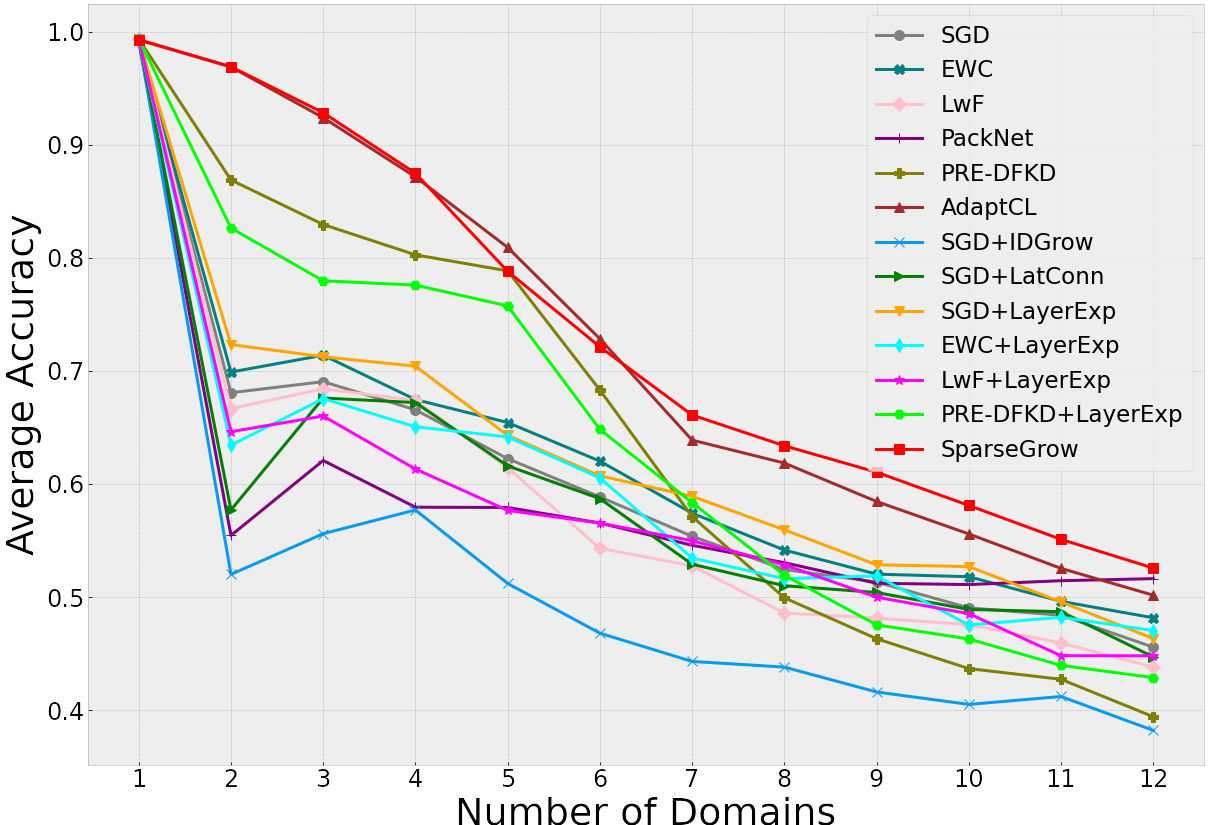
Figure 3: Average accuracy fluctuation of different methods across an increasing number of observed domains. Methods include CL baselines, model growth techniques, and CL methods+LayerExp. Rehearsal methods like LwF and PRE-DFKD initially decline when combined with LayerExp, indicating potential unsuitability for directly applying LayerExp and the risk of increased GIFt; later, LayerExp positive effects outweigh the negative impact of GIFt as domains increase. SparseGrow excels in knowledge retention, with its effectiveness improving as the number of domains rises.

Table 2: Comprehensive evaluation of baselines in terms of AAC, BWT, and FWT on twelve domains of Permuted MNIST. Comparison includes: 1) Simple baselines, 2) SGD with model growth techniques IDGrow, LatConn, LayerExp and 3) Baselines with LayerExp.

Method	AAC↑	BWT↑	FWT↑
SGD	0.4556	-0.5739	0.0493
EWC	0.4816	-0.5454	0.0638
LwF	0.3976	-0.6387	0.0540
PackNet	0.5163	-0.5049	0.0659
PRE-DFKD	0.3941	-0.6392	0.0774
AdaptCL	0.5016	-0.2532	0.0865
SGD+LatConn	0.4474	-0.6799	0.0779
SGD+IDGrow	0.3822	-0.6532	0.1418
SGD+LayerExp	0.4632	-0.5658	0.0737
SGD+LayerExp+ODInit	0.4683	-0.5598	0.0742
EWC+LayerExp	0.4703	-0.5571	0.0597
LwF+LayerExp	0.3941	-0.6426	0.0680
PRE-DFKD+LayerExp	0.4064	-0.6248	0.0759
EWC+LayerExp+ODInit	0.4755	-0.5498	0.0594
LwF+LayerExp+ODInit	0.3971	-0.6405	0.0668
PRE-DFKD+LyExp+ODInit	0.4199	-0.6196	0.0747
SparseGrow	0.5256	-0.2066	0.0974

Table 3: Performance evaluation of CL methods in terms of average accuracy (AAC), backward knowledge transfer (BWT), and forward knowledge transfer (FWT) on the domain-incremental datasets of FreshStale and DomainNet.

Method	FreshStale			DomainNet
	AAC↑	BWT↑	FWT↑	AAC↑	BWT↑	FWT↑
SGD+LayerExp	0.617	-0.450	0.027	0.464	-0.657	0.109
EWC+LayerExp	0.694	-0.360	0.039	0.463	-0.661	0.109
LwF+LayerExp	0.641	-0.424	0.009	0.434	-0.699	0.099
PRE-DFKD+LayerExp	0.703	-0.200	0.089	0.446	-0.475	0.090
SparseGrow	0.737	-0.273	0.049	0.624	-0.283	0.091

We conduct a comprehensive performance comparison of all baselines, including existing methods with and without model growth, on domain-incremental permuted MNIST datasets. Figure 3 depicts average accuracy fluctuation with an increasing number of tasks or domains for various baseline methods. The comparison between SparseGrow and AdaptCL emphasizes the importance of appropriate model growth in enhancing adaptability facing more domains, with only one expansion. Our model achieves the best performance, with its effectiveness improving as domain number rises. Comparison among growth strategies suggests that layer expansion consistently improves model accuracy, while lateral connections show unstable effects and in-depth growth mostly has negative impacts. Notably, rehearsal methods like LwF and PRE- DFKD exhibits an initial decline when combined with LayerExp, suggesting such techniques may not integrate well with layer expansion directly, possibly leading to more GIFt. Yet, the later positive effects of model capacity enhancement from expansion seem to surpass the negative impact of GIFt as domains increase. LwF’s average accuracy falls below SGD, suggesting that knowledge distillation methods may not be suitable for permuted MNIST that lack cross-domain similarity. For PackNet, the model’s average accuracy remains nearly constant as the number of domains increases. Incorporating on-data initialization into all baselines with layer expansion leads to improved AAC overall, indicating the effectiveness of this approach. Table 2 compares the AAC, BWT, and FWT metrics of three categories of CL models after learning from 12 domains consecutively. SparseGrow, in comparison to baselines, significantly mitigates overall forgetting issues, enhancing adaptability and surpassing SGD with LayerExp in BWT by 64% and AAC by 15%, demonstrating better knowledge retention. On-data initialization, when combined with layer expansion, shows consistent improvements on layer-expanded baselines such as SGD, EWC, LwF and PRE-DFKD, in AAC, BWT, and FWT, showing it as a generic approach. PackNet, utilizing static pruning, exhibits advantages with a larger number of datasets; however, its reliance on known total tasks numbers makes it unfeasible in CL scenarios.

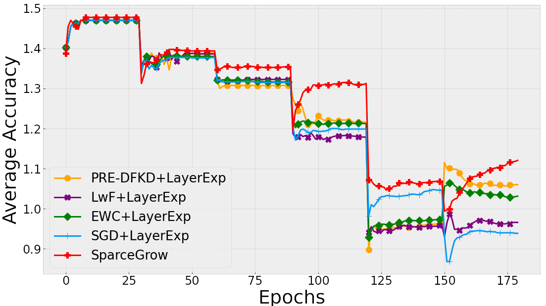
Figure 4: Epoch-wise average accuracy of observed domains using different continual learning methods with layer expansion on FreshStale datasets with six sequential domains.

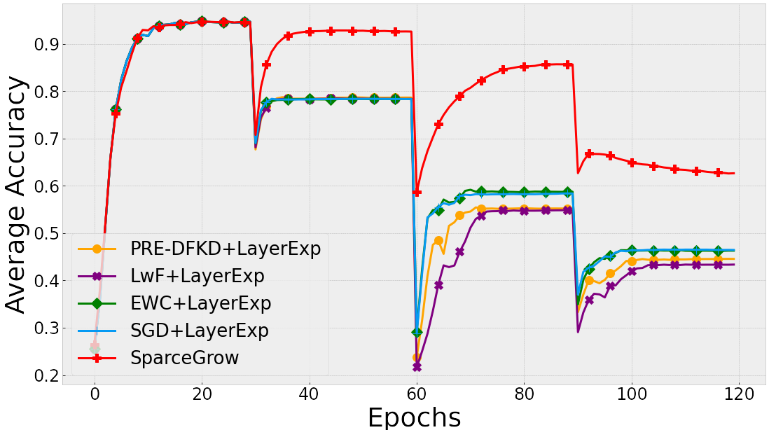
Figure 5: Epoch-wise average accuracy of observed domains using different continual learning methods with layer expansion on DomainNet datasets with four sequential domains.

Table 4: Comparison of average accuracy (AAC), backward knowledge transfer (BWT), forward knowledge transfer (FWT), and each dataset’s test accuracy using different CL methods in the most challenging class-incremental setting.

Method	AAC↑	BWT↑	FWT↑	Test Accuracy↑
				Class 0,1,2	2,3,4,5	0,3,6,7	6,8,9
SGD+LayerExp	0.309	-0.917	0.188	0.000	0.000	0.240	0.996
EWC+LayerExp	0.309	-0.917	0.188	0.000	0.000	0.240	0.996
LwF+LayerExp	0.309	-0.917	0.187	0.000	0.000	0.239	0.997
PRE-DFKD+LayerExp	0.330	-0.839	0.181	0.100	0.000	0.336	0.883
SparseGrow	0.412	-0.623	0.165	0.279	0.081	0.307	0.981

Addressing Growth-Induced Forgetting Evaluation

To assess the ability of different CL methods in reducing GIFt across diverse applications, we evaluated their layer-expanded versions (having GIFt) using the FreshStale and DomainNet datasets. Figure 4 and 5 visualizes the epoch-wise average accuracy (AAC) of different baseline methods on the FreshStale and DomainNet datasets. And Table 3 shows the AAC, BWT and FWT on the two application datasets. Figure 4 suggests that these CL methods can partially alleviate the effects of layer expansion-induced GIFt. SparseGrow consistently demonstrates the most stable reduction in model forgetting, achieving the highest AAC. In Figure 5, SparseGrow exhibits consistent effectiveness in combating GIFt, surpassing other methods in mitigating the effects induced by layer expansion when compared to SGD. Results in Table 3 reveal that existing regularization and rehearsal-based methods exhibit some effectiveness in addressing GIFt, but their performance across different datasets lacks consistency. In contrast, SparseGrow consistently minimizes the impact of growth-induced forgetting across these applications.

Class-Incremental Learning Setting Results

To assess the performance of our method in diverse task-agnostic settings, the methods were also evaluated in challenging class-incremental learning scenarios, as depicted in Table 4. In this setting, similar inputs lead to distinct classes assigned to different output layers, often resulting in rapid forgetting within a single epoch. Given the heightened intensity of forgetting and the scale of the datasets, techniques such as rehearsal and regularization methods struggle to effectively maintain accuracy, exhibiting only marginal superiority over SGD. In contrast, SparseGrow excels in preserving accuracy significantly, highlighting its potential in mitigating forgetting in task-agnostic environments.

Conclusion

Our study focuses on the crucial issue of growth-induced forgetting caused by improper model growth in task-agnostic continual learning. We have identified layer expansion as a promising fundamental model growth technique. Our proposed SparseGrow approach is specifically designed to boost adaptability and knowledge retention of layer expansion. Experimental validations have demonstrated the effectiveness of our method in mitigating growth-induced forgetting and improving knowledge retention for incremental tasks. Future research could aim to optimize the timing of model growth and leverage techniques such as neural architecture search to further enhance the model’s adaptability and overall performance with new data.

References

- Ardywibowo et al. (2022) Ardywibowo, R.; Huo, Z.; Wang, Z.; Mortazavi, B. J.; Huang, S.; and Qian, X. 2022. Varigrow: Variational architecture growing for task-agnostic continual learning based on bayesian novelty. In International Conference on Machine Learning, 865–877. PMLR.
- Binici et al. (2022) Binici, K.; Aggarwal, S.; Pham, N. T.; Leman, K.; and Mitra, T. 2022. Robust and resource-efficient data-free knowledge distillation by generative pseudo replay. In Proceedings of the AAAI Conference on Artificial Intelligence, volume 36, 6089–6096.
- Bottou et al. (1991) Bottou, L.; et al. 1991. Stochastic gradient learning in neural networks. Proceedings of Neuro-Nımes, 91(8): 12.
- Davis and Zhong (2017) Davis, R. L.; and Zhong, Y. 2017. The biology of forgetting—a perspective. Neuron, 95(3): 490–503.
- Deng, Aimone, and Gage (2010) Deng, W.; Aimone, J. B.; and Gage, F. H. 2010. New neurons and new memories: how does adult hippocampal neurogenesis affect learning and memory? Nature reviews neuroscience, 11(5): 339–350.
- Geng et al. (2021) Geng, B.; Yuan, F.; Xu, Q.; Shen, Y.; Xu, R.; and Yang, M. 2021. Continual Learning for Task-oriented Dialogue System with Iterative Network Pruning, Expanding and Masking. In Zong, C.; Xia, F.; Li, W.; and Navigli, R., eds., Proceedings of the 59th Annual Meeting of the Association for Computational Linguistics and the 11th International Joint Conference on Natural Language Processing (Volume 2: Short Papers), 517–523. Online: Association for Computational Linguistics.
- Hu et al. (2021) Hu, W.; Qin, Q.; Wang, M.; Ma, J.; and Liu, B. 2021. Continual learning by using information of each class holistically. In Proceedings of the AAAI Conference on Artificial Intelligence, volume 35, 7797–7805.
- Hu et al. (2023) Hu, Z.; Li, Y.; Lyu, J.; Gao, D.; and Vasconcelos, N. 2023. Dense network expansion for class incremental learning. In Proceedings of the IEEE/CVF Conference on Computer Vision and Pattern Recognition, 11858–11867.
- Hung et al. (2019) Hung, C.-Y.; Tu, C.-H.; Wu, C.-E.; Chen, C.-H.; Chan, Y.-M.; and Chen, C.-S. 2019. Compacting, picking and growing for unforgetting continual learning. Advances in Neural Information Processing Systems, 32.
- Joseph et al. (2021) Joseph, R.; Khatwani, N.; Sohandani, R.; Potdar, R.; and Shrivastava, A. 2021. Food Aayush: Identification of Food and Oils Quality. In Integrated Emerging Methods of Artificial Intelligence & Cloud Computing, 71–78. Springer.
- Kirkpatrick et al. (2017) Kirkpatrick, J.; Pascanu, R.; Rabinowitz, N.; Veness, J.; Desjardins, G.; Rusu, A. A.; Milan, K.; Quan, J.; Ramalho, T.; Grabska-Barwinska, A.; et al. 2017. Overcoming catastrophic forgetting in neural networks. Proceedings of the national academy of sciences, 114(13): 3521–3526.
- Kozal and Wozniak (2023) Kozal, J.; and Wozniak, M. 2023. Increasing depth of neural networks for life-long learning. Information Fusion, 98: 101829.
- Li et al. (2019) Li, X.; Zhou, Y.; Wu, T.; Socher, R.; and Xiong, C. 2019. Learn to grow: A continual structure learning framework for overcoming catastrophic forgetting. In International Conference on Machine Learning, 3925–3934. PMLR.
- Li and Hoiem (2017) Li, Z.; and Hoiem, D. 2017. Learning without forgetting. IEEE transactions on pattern analysis and machine intelligence, 40(12): 2935–2947.
- Liu et al. (2020) Liu, J.; Xu, Z.; Shi, R.; Cheung, R. C.; and So, H. K. 2020. Dynamic sparse training: Find efficient sparse network from scratch with trainable masked layers. arXiv preprint arXiv:2005.06870.
- Lopez-Paz and Ranzato (2017) Lopez-Paz, D.; and Ranzato, M. 2017. Gradient episodic memory for continual learning. Advances in neural information processing systems, 30.
- Madaan et al. (2023) Madaan, D.; Yin, H.; Byeon, W.; Kautz, J.; and Molchanov, P. 2023. Heterogeneous continual learning. In Proceedings of the IEEE/CVF Conference on Computer Vision and Pattern Recognition, 15985–15995.
- Mallya and Lazebnik (2018) Mallya, A.; and Lazebnik, S. 2018. Packnet: Adding multiple tasks to a single network by iterative pruning. In Proceedings of the IEEE conference on Computer Vision and Pattern Recognition, 7765–7773.
- Ostapenko et al. (2019) Ostapenko, O.; Puscas, M.; Klein, T.; Jahnichen, P.; and Nabi, M. 2019. Learning to remember: A synaptic plasticity driven framework for continual learning. In Proceedings of the IEEE/CVF conference on computer vision and pattern recognition, 11321–11329.
- Peng et al. (2019) Peng, X.; Bai, Q.; Xia, X.; Huang, Z.; Saenko, K.; and Wang, B. 2019. Moment matching for multi-source domain adaptation. In Proceedings of the IEEE International Conference on Computer Vision, 1406–1415.
- Rusu et al. (2016) Rusu, A. A.; Rabinowitz, N. C.; Desjardins, G.; Soyer, H.; Kirkpatrick, J.; Kavukcuoglu, K.; Pascanu, R.; and Hadsell, R. 2016. Progressive neural networks. arXiv preprint arXiv:1606.04671.
- Schwarz et al. (2018) Schwarz, J.; Czarnecki, W.; Luketina, J.; Grabska-Barwinska, A.; Teh, Y. W.; Pascanu, R.; and Hadsell, R. 2018. Progress & compress: A scalable framework for continual learning. In International Conference on Machine Learning, 4528–4537. PMLR.
- Shim et al. (2021) Shim, D.; Mai, Z.; Jeong, J.; Sanner, S.; Kim, H.; and Jang, J. 2021. Online class-incremental continual learning with adversarial shapley value. In Proceedings of the AAAI Conference on Artificial Intelligence, volume 35, 9630–9638.
- Xu and Zhu (2018) Xu, J.; and Zhu, Z. 2018. Reinforced continual learning. Advances in Neural Information Processing Systems, 31.
- Yan, Xie, and He (2021) Yan, S.; Xie, J.; and He, X. 2021. Der: Dynamically expandable representation for class incremental learning. In Proceedings of the IEEE/CVF conference on computer vision and pattern recognition, 3014–3023.
- Yang et al. (2021) Yang, L.; Lin, S.; Zhang, J.; and Fan, D. 2021. Grown: Grow only when necessary for continual learning. arXiv preprint arXiv:2110.00908.
- Yoon et al. (2017) Yoon, J.; Yang, E.; Lee, J.; and Hwang, S. J. 2017. Lifelong learning with dynamically expandable networks. arXiv preprint arXiv:1708.01547.
- Zhang et al. (2020) Zhang, J.; Zhang, J.; Ghosh, S.; Li, D.; Zhu, J.; Zhang, H.; and Wang, Y. 2020. Regularize, expand and compress: Nonexpansive continual learning. In Proceedings of the IEEE/CVF Winter Conference on Applications of Computer Vision, 854–862.
- Zhao, Saxena, and Cao (2023) Zhao, Y.; Saxena, D.; and Cao, J. 2023. AdaptCL: Adaptive continual learning for tackling heterogeneity in sequential datasets. IEEE Transactions on Neural Networks and Learning Systems.