Optimizing the - Relation of HII Galaxies for Improving Cosmological Application
Abstract
The basic premise of using HII starburst galaxies (HIIGs) as cosmic “standard candels” is that there is a significant correlation between the H luminosity () and the velocity dispersion () of the ionized gas from HIIGs measurements, which can be called as the empirical - relation. However, the scaling - relation well-calibrated with the lower-redshift HIIGs is unfitted for the higher-redshift HIIGs. To solve this problem, we explore new relational expression for the - relation which should be suitable for both lower-redshift and higher-redshift HIIGs. After reconstructing the Hubble diagram with the Gaussian process (GP) method from the Pantheon+ supernovae Ia sample, we examine and compare six different revised formulas of - relation. Furthermore, we use the Bayesian evidence to compare the revised - relations with the analysis of a joint sample of 36 giant extragalactic HII regions (GEHRs) and 145 HIIGs. It turns out that the redshift-dependent bilinear correction and the quadratic based correction are significantly better than the others. Moreover, a quadratic based correction is the most supported one. It suggests that the appropriate corrections to the - relation should be considered when the HIIGs are used as a kind of cosmological probes.
I Introduction
HIIGs are compact low mass dwarf irregular galaxies. Due to the difficulty in detecting their underlying galactic spectra, their emission lines are almost entirely dominated by young (the age 5 Myr) massive star-forming regions [1, 2]. Through observational data selection, i.e. the largest equivalent width (EW) in their emission lines, HIIGs are extragalactic star-forming systems with the strongest narrow emission lines [3, 4, 5, 2]. This data selection also eliminates the influence of stellar formation models on their dominant luminosity, suggesting that the observed quantities of these cosmological distance galaxies have the same statistical characteristics [4]. Furthermore, due to the kinematics of the star formation process, it can be inferred that there is a correlation between the velocity dispersion of the ionized gas measured from their spectra and the system’s emission luminosity [6, 1]. The existence of the significant correlation between and , i.e., the empirical - relation, opens up the possibility for HIIGs to serve as standard candles, which can become a kind of promising cosmological probes.
If the empirical relation between luminosity and velocity dispersion ( - relation) is physical, we can use GEHRs as a nearby sample to calibrate HIIGs [7, 8, 9, 10]. GEHRs are nearby star-forming regions with spectral characteristics identical to HIIGs, typically located in the outer disks of late-type galaxies. Through standard candles such as Cepheid variables or well-measured distance indicators, which can combine GEHRs with low-redshift HIIGs to study the form of the empirical relation and complete the calibration [6, 11, 12, 13, 3]. This allows HIIGs as a forward distance ladder, to study the history of cosmic evolution and the properties of various components dominating cosmic evolution to [14, 15, 16, 17, 18, 19, 20, 21, 22, 23, 24].
The usage of HIIGs as standard candles heavily relies on the - relation, and the empirical - relation has been widely discussed over the past few decades [6, 11, 25, 1]. Notably, Chávez et al. [1] used the Subaru High Dispersion Spectrograph, European Southern Observatory Very Large Telescope Ultraviolet and Visual Echelle Spectrograph, and the Sloan Digital Sky Survey DR7 spectroscopic catalogue [26] to obtain a sample of 128 low-redshift HIIGs to discuss the linear empirical relation between the velocity dispersion and luminosity of HIIGs. They also analyzed the corrections to the linear empirical formula based on parameters such as the colour, the masses, the metallicity, or the age of the starburst [27, 28, 6, 11].
The local analysis of the linear empirical relation is systematic and comprehensive, but extending this empirical relation, which is only discussed in low-redshift sample, directly to higher redshifts remains uncertain [16, 29, 30]. In fact, this is a self-contradictory discussion. If the cosmological model and its parameters are unknown, we generally can not obtain the luminosity distances of high-redshift HIIGs, and thus can not discuss the - relation at high redshifts. In this case, assuming that the local empirical relation still holds at high redshifts is a direct and unavoidable operation, similar to using supernovae as standard candles to study the history of cosmic evolution [31, 32, 33, 34, 35, 36, 37]. This has also become a main route to discuss and explain the tension and tension [38, 39, 40, 41, 42].
Recently, Cao and Ratra [29] used HIIGs data combined with the cosmic chronometer H(z) and Baryon Acoustic Oscillation (BAO) data [43] to discuss the evolution of the empirical formula for HIIGs as standard candles under six cosmological models. They found that although HIIGs can still be standardized, their - relation indeed presents different situations at low and high redshifts. This is a very significant conclusion, suggesting a possible scheme to improve the relation and to make HIIGs becoming a kind of reliable cosmological probes. However, discussions based on cosmological models complicate the - relation problem of HIIGs. We can not determine whether this deviation comes from HIIGs themselves, nor can we quantify the impact of cosmological models on the results. This is especially problematic given that various cosmological models are currently challenged, and these cosmological models may not describe our universe well.
In this paper, we reconstructed the Hubble diagram via employing the GP method and Pantheon+ SNe Ia sample [44]. Since the correction to the - relation may be caused by multiple factors, we analyze the effect of the sample used to reconstruct the Hubble diagram and the possible effects of detector selection bias from different observational sources of HIIGs. After excluding the influence of these issues, we discuss the consistency between the GEHRs and HIIGs data in fitting the classic scaling - relation, and explore some possible corrections to the scaling relation, and analyze the results based on various statistical indicators.
The rest of the paper is organized as follows. In Sec. II, we introduce the various datasets used in this paper. In Sec. III, we explain the fitting methods used and provide the reconstructed distance modulus . In Sec. IV, we use bin-wise fitting to discuss the impact of calibration datasets and possible detector selection effects on the - relation. In Sec V, based on our analysis of the data, we derive possible corrections to the - relation. We perform maximum likelihood estimation for different - relations, analyze the posterior parameters, examine the results using Bayesian evidence, and provide necessary discussions based on our work and analyze its limitations. Sec VI is the summary of the entire paper.
II Selection of Observational Dataset
II.1 GEHRs and HIIGs
In this paper, we use a sample with 36 GEHRs and 181 HIIGs to analyze the - relation. The - calibrated with the GEHRs is alway used in the cosmologica application of HIIGs [3, 5, 2, 24]. The observational quantities of these samples can be obtained through methods such as spectral analysis to acquire the emission line fluxes and velocity dispersion .
The GEHRs sample with 36 data point is from Fernández Arenas et al. [3]. These luminosities are calculated using the distance information provided by local standard candles or distance indicators (see Table.1 in Fernández Arenas et al. [3]), which can be obtained from the following equation,
| (1) |
where [Mpc] is the luminosity distance, and its relation with the distance modulus is
| (2) |
The error analysis of luminosity in Fernández Arenas et al. [3] includes the distance errors of distance indicators and the extinction and absorption of observed flux [45, 46, 1]. The calculation of velocity dispersion has removed the effects of thermal, fine structure constants, and instrumental broadening. Similar or identical discussions are also detailed in the analysis of the HIIGs data.
The HIIGs sample with 181 data point used are from González-Morán et al. [2], which includes 107 local HIIGs [1] and 74 high-redshift HIIGs [5, 4, 2]. In fact, the redshift distribution of these samples is not uniform. The redshift range of the local sample is , while the high-redshift sample range from , mainly concentrated in two intervals: and . We will consider using part of the samples to discuss issues based on practical considerations such as the characteristics of the calibration samples and the Gaussian process. The observational sources of these 181 HIIGs are also diverse, which can be referenced in Table 2 of González-Morán et al. [2]. We will discuss the impact of detector selection effects in Sec. IV
II.2 SNe Ia
SNe Ia are widely used standard candles, applied in cosmological studies such as cosmological model parameter constraints based on the relation between their apparent magnitude and redshift measurements. In this paper, we use the Pantheon+ sample, which includes 1701 light curves of 1550 distinct SNe Ia from 18 different sky surveys, with a redshift range of [44]. To avoid data degeneracy brought by local calibrations such as Cepheid variables, we only use SNe Ia sample with to reconstruct the Hubble diagram . The distance modulus is defined as
| (3) |
where is the corrected apparent magnitude of the SNe Ia, calculated using the SALT2 method [33, 47, 48, 44, 49], and is the absolute magnitude. In this paper, the prior for the absolute magnitude of supernovae is set to the result calibrated by Cepheid variables as used by SH0ES, corresponding to [50].
III Gaussian Process Method and Bayesian Formula
In all analyses of this paper, we used two statistical methods to obtain the required physical quantities and their errors. These include using the GP to reconstruct the distance modulus without relying on cosmological models, and using the Nested sampling based on Bayesian formula to obtain the posterior distribution of the parameters of - relation and its correction relation. We briefly present the basic theory of the GP method and Bayesian formula, the specific situations under the research problems in this paper, and the code used for numerical solutions.
III.1 Gaussian Process and The Reconstruction of The Distance Modulus
Gaussian process (GP) is a generalization of the Gaussian distribution over continuous variables, and it is a method for reconstructing functional relations between physical quantities without relying on specific functional forms. If a univariate function follows a Gaussian process, then at any satisfies a Gaussian distribution with mean and variance , and the covariance between different is , then this Gaussian process can be represented as
| (4) |
where the correlation function is essentially a kernel function. More detailed descriptions and proofs of Gaussian process can be found in Rasmussen and Williams [51], and GP are also widely applied in cosmology [52, 53, 54]. The GP in this paper is implemented using the open-source Python code GaPP3 [53], which marginalizes the conditional probability distribution to obtain hyperparameters through the optimization algorithm, resulting in the distribution image of the predicted set.
When using GP to reconstruct the distance modulus, Mu et al. [55] discussed the advantages of applying the double squared exponential kernel function to the Pantheon+ sample. Its form is
| (5) |
where are referred to as hyperparameters. Clearly, the correlation strength parameters and dominate the scale of the covariance matrix of , while the correlation length parameters and dominate the correlation length between different .
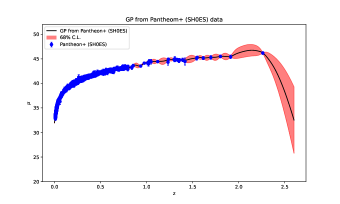
The kernel function in Eq. 5, has maximum likelihood for the Pantheon+ sample calibrated by SH0ES. Therefore, we follow Mu et al. [55] and use this kernel function for the covariance matrix of the joint errors of the Pantheon+ sample in this paper. The reconstructed distance moduli are shown in Fig. 1.
In Fig. 1, the Hubble diagram reconstructed using GP shows some oscillations in the central values of the distance modulus over a certain interval. In subsequent comparative studies, when using another supernova absolute magnitude prior (MLCS prior), these oscillations are significantly reduced, and none of the analysis results in the entire paper are affected by these oscillations. This is also related to the fact that the oscillation interval has a larger error.
The luminosity errors of the HIIGs calculated using the following formula absorb the additional errors caused by the oscillations.
| (6) |
where the and are the error of the distance modulus and the log emission line fluxes . It should be noted that although our method does not depend on cosmological models, using Eq. 1 and Eq. 2 to calculate luminosity relies on the cosmological principle, i.e., the assumption of homogeneity and isotropy of the universe on large scales. We assume that the universe has the same distance modulus in different directions at the same redshift.
III.2 Bayesian Formula and Nested Sampling
According to Bayesian theory, the parameter probability distribution of the posterior is proportional to the probability distribution of the data, which can be written as
| (7) |
where is the likelihood function, is the prior probability distribution of the parameters, is the Bayesian evidence, which is also the normalization coefficient of the posterior distribution function.
In this paper, we used the open-source Python code PyMultiNest to perform Nested sampling, in order to obtain the posterior distribution function and Bayesian evidence [56, 57]. This program serves as an interface to the MultiNest algorithm [58].
The prior distribution of the parameters is set as a uniform distribution. For the classic scaling - relation
| (8) |
where the parameter priors and are respectively. For the correction parameters that exist in different relations, we set all of them to . The likelihood function under any relation can be expressed as
| (9) |
where the theoretical formulas for calculating are different for each case, and the corresponding errors also differ. Here, we present the case for the scaling - relation, which
| (10) |
corresponding to Eq. 8. We will present the situations under different forms of corrections discussed in Sec. V.
IV The Impact of Different Calibration Samples and Detector Selection Effects
IV.1 Possible Sources of Parameter Deviation in Different Redshift Ranges
Regarding Fig.3 in Cao and Ratra [29], the reasons for different parameters of - relation at low and high redshifts can be further discussed.
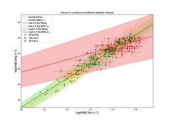
In this paper, through the selection of datasets and fitting methods, we first avoid the influence of cosmological models on the - relation of HIIGs. Here, we only use 36 GEHRs and 145 HIIGs with redshifts between , all of which are within the stable Hubble diagram redshift range of the Pantheon+ sample in Fig. 1. The 145 HIIGs data are divided into 106 low-z HIIGs and 39 high-z HIIGs. The results of constraining the scaling - relation from three bins are shown in Fig. 2.
Although the - parameters at high redshifts have larger errors due to the limited samples and concentration in a smaller velocity dispersion range, it can still be noticed that there is indeed a deviation between high-redshift and low-redshift samples. This includes significant differences in mean values, and the fact that most of the GEHRs data falls outside the 1- range of the high-redshift sample, despite such large error ranges. Our results, which are independent of cosmological models, indicate that the issues present in Fig.3 of Cao and Ratra [29] under six cosmological models still exist, and the parameter deviation in different redshift ranges is unrelated to cosmological models.
In addition, it should be noted that the reasons leading to the parameter deviation in Fig. 2 may be multifaceted. We analyze the following points: (1) Whether HIIGs data under different calibration samples all show inconsistencies in the - relation; (2) Since the HIIGs data at different redshifts come from observations by different telescopes, and the high-redshift sample have different sources, could the redshift evolution of the classic relation be a telescope selection effect? (3) Whether there are possible corrections to the - relation, noting that such corrections may come from two aspects: redshift correction or form correction to the classic relation, because as redshift increases, velocity dispersion also increases.
IV.2 Calibration Samples and Detector Selection Effects
To control variables in analyzing the problem, we will calculate luminosities based on the distance moduli reconstructed from different datasets and the flux of HIIGs, and analyze HIIGs data from different observational sources separately to eliminate as much as possible the problems brought by calibration samples.
Considering that the local measurement of will affect the intercept in the - relation, and consequently influence the slope or correction parameters in the - relation through parameter degeneracy, we need to analyze the impact of different SNe Ia absolute magnitudes from various local calibrations on the - relation. The impact of different priors on has been discussed by Chen et al. [59] in detail. We will use two different absolute magnitudes for supernovae: (referred to as the SH0ES prior in this paper) calibrated by Cepheid variables [50], and (referred to as the MLCS prior in this paper) given by the Multicolor Light Curve Shape (MLCS) method [60].
Another commonly used dataset is cosmic chronometers (CCs) [61, 62, 63, 64, 65, 66, 67, 65]; however, reconstructing the Hubble diagram from CCs requires integrating the Hubble parameter from 0 to , which decreases the reliability of the resulting central of the distance modulus. Additionally, calculating the distance modulus via luminosity distance significantly amplifies the luminosity errors for low-redshift HIIGs. These two reasons led us to abandon using CCs as a calibration sample for HIIGs. Therefore, our results rely on the assumption of supernovae as standard candles.
For the detector selection effects, the 145 HIIGs data at include 106 local HIIGs data from the same source and 39 high-redshift HIIGs data. Among the 39 high-z data, 4 are from Xshooter, with 3 out of 4 at ; 7 data are from literature; 13 data are from MOSFIRE, with redshift range ; 15 data are from KMOS, with redshift range . We categorize these data, dividing the 106 local HIIGs data into two bins at . These two bins allow us to notice whether there are inconsistent linear relations for the same detector at close redshifts, which can to some extent illustrate the characteristics of redshift evolution or the possibility of higher-order corrections to the - relation. For high-redshift HIIGs, the Xshooter sample is too small and its redshift is inconsistent with other data, making it difficult to draw conclusions about the - relation parameters. 7 literature data come from different telescopes can not illustrate the possible impact of selection effects. Therefore, we only use the 13 MOSFIRE and 15 KMOS data, dividing them into two bins based on observational sources. It’s worth noting that the redshift distributions of these two bins are close, and their velocity dispersion distributions are also relatively close.
The results of using Pantheon+ sample with the SH0ES prior to constrain the linear - relation parameters are shown in Fig. 3, where the parameters are plotted using the mean values of the posterior distributions. For the bin-wise analysis, the sample size of each bin is significantly reduced, and the velocity dispersion distribution range is smaller, resulting in larger errors in the parameter posteriors. Therefore, we only use the mean values here to judge the telescope selection effects and further analyze the evolutionary characteristics of the - relation.
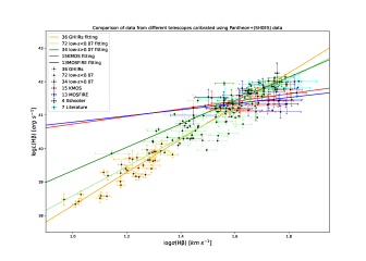
Fig. 3 shows the results calibrated by Pantheon+ sample with the SH0ES prior. We observe a ”seesaw” behavior in the linear fits across different bins: as redshift and velocity dispersion increase, the slopes of the fitted lines decrease, and the intercepts increase. We also reconstructed the Hubble diagram using the MLCS prior to control variables, including a qualitative analysis of CCs data. All three calibration samples yielded consistent results. Low-redshift samples from the same dataset show inconsistent - relations across different redshift (and ) intervals. Meanwhile, high-redshift HIIGs, which are closer in redshift and , show nearly consistent posterior mean values of the - relation, even though they were observed by different detectors. This suggests that the observed evolution effect is unlikely due to calibration samples or detector selection effects, but its inherent characteristic.
The evolution itself may be twofold. One direct possibility is that the - relation parameters are different at different redshifts, i.e., there exists a redshift-related correction term. This inference is straightforward, but this evolution can hardly explain why the - relation changes rapidly within a not-so-different redshift range in the local HIIGs sample, it may point to an - relation that includes more than just redshift evolution. Noting that the velocity dispersion of the local HIIGs sample is generally larger than that of the HIIGs sample and has a velocity dispersion range close to the high-redshift sample, we speculate that another possible situation is that the - relation needs high-order correction.
V Comparing the revised formulas of - relation
V.1 Possible Correction Mechanisms and Theoretical Forms
The linear assumption for the classic - relation of GEHRs and HIIGs has been similarly conjectured for the GRB dataset [68, 69, 70, 71], another potential standard candle. For example, the well-known Amati relation for GRBs, and the hypothesis about its redshift evolution has been discussed multiple times [72, 73]. When considering the redshift evolution correction of the - relation for HIIGs, we base it on its own possible sources of redshift evolution, while also drawing analogies from the redshift correction form of the Amati relation for GRBs.
In the discussion of the - relation, Chávez et al. [1] analyzed the influence of different observational parameters on the scaling relation based on local HIIGs sample at low redshifts. They found that incorporating other observables such as galaxy size or mass could reduce the systematic error when fitting the - relation. Considering that the formation of large-scale cosmic structures may cause these parameters to change with redshift, we denote the evolution parameter as and the possible redshift evolution correction term as . Thus, we have
| (11) | ||||
where . The third equality can be explained as follows, if we believe that the - relation in Sec.7 of Chávez et al. [1] inherently includes a part of parameter , and we still use Eq. 8 for cosmological studies, then in the above equation is actually in Eq. 8. Similar to all past operations, is viewed as a constant absorbed into , which is equivalent to accepting the increase of an rms scatter from to due to the limitation of observational data, ignoring the influence of more parameters. This is the unavoidable cost of treating the dispersed as a constant. Under this assumption, the correction brought by redshift evolution only has the latter term. We only consider the first-order term of , and set , then correction of - relation (labelled as “-correction”) corresponds to
| (12) |
It should be noted that this correction form only considers one parameter evolving with redshift, or in other words, the redshift evolution trend of one of the parameters is significantly greater than that of the others. A special case of the Eq.12 is when the redshift evolution parameter is the velocity dispersion itself. In this case, the added correction of - relation (labelled as “-correction”) is
| (13) |
Under these two corrections, the likelihood function form is consistent with the classic relation, and is still given by Eq. 10.
Another mechanism may also cause the - relation to be affected by redshift evolution. The ionization luminosity of young star clusters is influenced by their age, relatively stable before years, but changing rapidly afterwards. Fernández Arenas et al. [3] considered the impact of this situation using equivalent width. In this paper, on the other hand, consider that the universe is at different evolutionary stages at different redshifts, which causes the observed galaxies to have statistically varying characteristics in terms of their age with redshift, thereby affecting their ionization luminosity. We assume a redshift evolution on the luminosity exponential term, i.e., . Then, for the - relation, its evolutionary form is
| (14) |
then
| (15) |
We only consider the first-order term of redshift, so there exists a linear correction for redshift in the classic - relation. Here, we adopt the same form as in the redshift correction of the GRB Amati relation, the luminosity correction of - relation (labelled as “-correction”) is
| (16) |
A more general form, where these two parameters evolve with redshift in different ways, the bilinear correction of relation (labelled as “Bilinear-correction”) corresponds to
| (17) |
In this two cases, the new likelihood function form is still Eq. 9. From the above equation, we can calculate for two situations.
In addition, we discussed the linear fitting of different data and found the velocity dispersion of HIIGs data themselves are correlated. Combining the distribution trend of all data, it looks more like a quadratic function. Therefore, we add a quadratic term to the classic scaling relation as a higher-order correction. The quadratic correction of relation (labelled as “Quadratic-correction”) is
| (18) |
In this case, the error term in the likelihood function is .
V.2 Model Selection Criteria
To compare the classic - relation and the five corrections mentioned in Sec. V.1, we consider using Bayesian evidence as judgment criteria to analyze the advantages of different corrections over the classic - relation, and calculate the systematic error corresponding to the best fit for each model.
Bayesian evidence as a model criterion [74, 75], which is the integral mentioned earlier in Sec. III.2. It considers the probability distribution including model parameter priors. In this paper, we actually used normal priors, but considering that some corrected relations may obtain unphysical maximum likelihood points in Nested sampling, we use the Bayesian evidence that considers the integral of the posterior distribution function for discussion.
The ratio of Bayesian evidence is an indicator for measuring models. In this paper, we calculate the Log-Bayesian evidence () and relative log-Bayesian evidence (), where is the Log-Bayesian evidence of classic - relation. correspond to inconclusive, weak, moderate, and strong evidence, respectively, and the model with greater log-Bayesian evidence is preferred [75].
In addition, we also calculated the systematic error of the model fitting the data based on the relation between and the degrees of freedom of the system. Generally, equals the degrees of freedom, i.e. , where is the number of model parameters, represents the number of observed data points. We calculate the systematic error that satisfies when added, using the parameter values at maximum likelihood. The term is included as part of in the calculation, and the final value is used to determine .
In GRB parameter constraints, the parameter as systematic error participates jointly in Bayesian estimation, but we did not operate like this here. This is because we can not determine how to change the likelihood function for a free parameter that only appears in the error term in a multi-parameter situation. Adding this error parameter can only ensure that the model with this parameter can obtain maximum likelihood estimation, but it can not satisfy , which will increase the difficulty of discussion.
V.3 Results and Discussion
| Models | |||||||
|---|---|---|---|---|---|---|---|
| Classic - relation | |||||||
| -correction | |||||||
| -correction | |||||||
| -correction | |||||||
| Bilinear-correction | |||||||
| Quadratic-correction |
In this section, we present the posterior estimation results for all - relations mentioned in Sec. V.1, using 36 GEHRs and 145 HIIGs calibrated by Pantheon+ sample with SH0ES prior. The posterior results are given in Table. 1. The relevant parameters used for analyzing statistical results are obtained by the methods described in Sec. V.2. The tables provide the mean values and confidence intervals of the parameter posteriors.
Table. 1 shows the results under Pantheon+ sample with the SH0ES prior. Due to the additional parameters introduced by the corrected models compared to the classic - relation, we can see that they all reduce systematic errors. However, it’s important to note that the effectiveness of the first three corrections in reducing systematic errors is quite low, and from the Bayesian evidence perspective, comparing with the classic model, none of three models with redshift corrections for parameter , velocity dispersion parameter , and luminosity have an advantage. Therefore, these three models do not have consistently significant conclusions for today’s data compared to the classic scaling relation, and adding a redshift-related parameter is not very attractive.
The exciting correction models are the bilinear correction model and the quadratic correction model. These two models are superior to the classic - relation. When fitting the quadratic correction model, due to the posterior distribution of the parameter deviating far from the parameter under the classic scaling relation, we relaxed the parameter prior of . The posterior results also indicate that this so-called correction relation deviates too much from the classic relation. The original parameters and are inconsistent at the confidence interval, and the ”correction” parameter also excludes at the confidence interval. Although its behavior no longer resembles a correction to the classic - relation, this functional form has very strong evidence in terms of statistics, and calculating systematic errors reveals that this relation greatly reduces systematic errors. All of the above indicate that this relation fits the data well.

In Fig. 4, we show the fit of the quadratic correction model to the data. Compared to the classic relation, although the posterior distribution of the parameters in the corrected relation varies significantly, it still acts as a correction within the velocity dispersion range of the data. For larger ranges, the quadratic correction model reduces the slope of the curve. The inclusion of an additional correction parameter increases the statistical uncertainty in the empirical relation, but the and confidence intervals of the quadratic correction model align better with expectations compared to the classic - relation. Almost all the data points fall within the range of the quadratic correction model, whereas a significant portion of the data exceeds the confidence interval of the classic - relation. This also results in a reduction of the value, indicating that the corrected model reduces systematic errors. As the amount of HIIGs data increases in the future, whether this statistical characteristic will strengthen or weaken will help us better assess the reliability and necessity of the quadratic correction.
The results of the bilinear correction do not have the problem of completely deviating from the correction. From the parameter posterior intervals, we can see that its and are still near the classic relation, and the redshift evolution term provides a very effective correction. The two evolution coefficients and exclude at a confidence interval exceeding , confirming the redshift evolution of the - relation. The Bayesian evidence show that this correction model is superior to the scaling - relation, and this model also effectively reduces systematic error. Besides, although the quadratic correction model is a three-parameter model and the bilinear correction model is a four-parameter model, in fact, the model with redshift evolution correction has stronger constraints in terms of physical origin and parameter degrees of freedom. Although we can not derive this model from first principles, it is not entirely empirical.
In addition, we performed the same tests using the Pantheon+ sample with the MLCS prior, and the results are completely consistent with the conclusions from Table. 1, ruling out the influence of sample selection effects. Since the Hubble diagram reconstructed under MLCS prior is smoother, the same conclusion also indicates that the fluctuations in the high-redshift Hubble diagram do not affect the conclusions of this paper.
Our analysis shows that the - relation of HIIGs with based on cosmology-independent data and methods. We found that compared to the classic - relation Eq. 8, the bilinear redshift-corrected relation Eq. 17 and the quadratic-corrected relation Eq. 18 fit the HIIGs data better. When using HIIGs as cosmological probes, the impact of these corrections needs to be considered. In addition, today’s HIIGs sample are not relatively uniformly distributed in redshift space and velocity dispersion space. This may lead to research results akin to drawing an elephant with four parameters. This requires more samples to be observed in velocity dispersion space and redshift space, as also shown in Cao and Ratra [29]’s analysis results.
Apart from this approach, Melnick and Telles [76] attempted to reduce the scatter in the HIIGs - relation by correcting for luminosity evolution using a different method, but it was not very effective. In contrast, the quadratic correction in this paper significantly reduces systematic errors, although empirical formulas without a physical mechanism still face issues. A major weakness is that additional parameters can always be added to correct the classic relation, which is not the best solution. As data increases, the reliability of such bilinear correction and quadratic correction will be further tested.
VI Summary
In this work, we use the Gaussian process to reconstruct the Hubble diagram with the Pantheon+ SNe Ia sample. On this basis, we then analyze and optimize the relation, which is an important foundation for the cosmological application of HIIGs. The process can avoid the dependence on the cosmological model. In particular, we explore and compare several possible and necessary corrections to the classic scaling relation for HIIGs.
We have proved the validity of the result from Cao and Ratra [29], which shows that the HIIGs in different redshift ranges indeed obtain different slopes for the scaling - relation. Remarkably, Cao and Ratra [29] obtain the same result in the frameworks of six different cosmological models, while our result is independent of cosmological model.
Furthermore, in Sec. IV, we analyze the possible sources of - relation bias, namely the dependence on calibration samples, detector selection effects, and corrections to the scaling - relation. For different calibration samples, we did not find that the bias in the - relation of HIIGs comes from detector selection effects. This analysis was conducted at the observational stage, and in this paper we have conducted another analysis from the perspective of the - relation.
For the - relation that has been discussed in detail using local sample [1], we extended this discussion to high-redshift sample based on the method in this paper, and analyzed possible correction forms of the - relation based on the physical mechanisms of HIIGs and data distribution. Under the comparison of the Bayesian evidence and systematic errors, we found that under different calibration samples, both the bilinear corrected - relation and the quadratic corrected - relation are significantly superior to the classic scaling - relation. When considering HIIGs as a kind of reliable standard candles and applying them to cosmological research, these two possible corrections should be discussed.
It should be noted that our analysis also has limitations. Our results depend on the standard candle assumption of SNe Ia and the cosmological principle, and our results are obtained on a small and unevenly distributed sample. All these factors limit our conclusions. Improvements to these shortcomings require more data to be observed in different redshift ranges or different velocity dispersion intervals. We look forward to the release of more HIIGs data, which will be decisive for the HIIGs cosmology.
Acknowledgements.
This work has been supported by the National Key Research and Development Program of China (No. 2022YFA1602903), and the National Natural Science Foundation of China (Nos. 12075042 and No. 11675032).References
- Chávez et al. [2014] R. Chávez, R. Terlevich, E. Terlevich, F. Bresolin, J. Melnick, M. Plionis, and S. Basilakos, The L– relation for massive bursts of star formation, Mon. Not. Roy. Astron. Soc. 442, 3565 (2014), arXiv:1405.4010 [astro-ph.GA] .
- González-Morán et al. [2021] A. L. González-Morán, R. Chávez, E. Terlevich, R. Terlevich, D. Fernández-Arenas, F. Bresolin, M. Plionis, J. Melnick, S. Basilakos, and E. Telles, Independent cosmological constraints from high-z H ii galaxies: new results from VLT-KMOS data, Mon. Not. Roy. Astron. Soc. 505, 1441 (2021), arXiv:2105.04025 [astro-ph.CO] .
- Fernández Arenas et al. [2018] D. Fernández Arenas, E. Terlevich, R. Terlevich, J. Melnick, R. Chávez, F. Bresolin, E. Telles, M. Plionis, and S. Basilakos, An independent determination of the local Hubble constant, Mon. Not. Roy. Astron. Soc. 474, 1250 (2018), arXiv:1710.05951 [astro-ph.CO] .
- Terlevich et al. [2015] R. Terlevich, E. Terlevich, J. Melnick, R. Chávez, M. Plionis, F. Bresolin, and S. Basilakos, On the road to precision cosmology with high-redshift H II galaxies, Mon. Not. Roy. Astron. Soc. 451, 3001 (2015), arXiv:1505.04376 [astro-ph.CO] .
- González-Morán et al. [2019] A. L. González-Morán, R. Chávez, R. Terlevich, E. Terlevich, F. Bresolin, D. Fernández-Arenas, M. Plionis, S. Basilakos, J. Melnick, and E. Telles, Independent cosmological constraints from high-z H ii galaxies, Mon. Not. Roy. Astron. Soc. 487, 4669 (2019), arXiv:1906.02195 [astro-ph.GA] .
- Terlevich and Melnick [1981] R. Terlevich and J. Melnick, The dynamics and chemical composition of giant extragalactic H II regions, Monthly Notices of the Royal Astronomical Society 195, 839 (1981), https://academic.oup.com/mnras/article-pdf/195/4/839/4861512/mnras195-0839.pdf .
- Sandage [1962] A. Sandage, The Distance Scale, in Problems of Extra-Galactic Research, Vol. 15, edited by G. C. McVittie (1962) p. 359.
- Melnick [1977] J. Melnick, Velocity dispersions in giant H II regions: relation with their linear diameters., Astrophys. J. 213, 15 (1977).
- Melnick [1978] J. Melnick, Velocity Dispersions in Giant H II Regions II. Relations with the Absolute Luminosities of the Parent Galaxies, 70, 157 (1978).
- Kennicutt [1979] J. Kennicutt, R. C., H II regions as extragalactic distance indicators. I. Observations and structural considerations., Astrophys. J. 228, 394 (1979).
- Melnick et al. [1987] J. Melnick, M. Moles, R. Terlevich, and J.-M. Garcia-Pelayo, Giant H II regions as distance indicators - I. Relations between global parameters for the local calibrators., 226, 849 (1987).
- Melnick et al. [1988] J. Melnick, R. Terlevich, and M. Moles, Giant H II regions as distance indicators- II. Application to H II galaxies and the value of the Hubble constant., 235, 297 (1988).
- Chávez et al. [2012] R. Chávez, E. Terlevich, R. Terlevich, M. Plionis, F. Bresolin, S. Basilakos, and J. Melnick, Determining the Hubble constant using giant extragalactic H ii regions and H ii galaxies, Monthly Notices of the Royal Astronomical Society: Letters 425, L56 (2012), https://academic.oup.com/mnrasl/article-pdf/425/1/L56/56939527/mnrasl_425_1_l56.pdf .
- Chávez et al. [2016] R. Chávez, M. Plionis, S. Basilakos, R. Terlevich, E. Terlevich, J. Melnick, F. Bresolin, and A. L. González-Morán, Constraining the dark energy equation of state with H II galaxies, 462, 2431 (2016), arXiv:1607.06458 [astro-ph.CO] .
- Leaf and Melia [2018] K. Leaf and F. Melia, A two-point diagnostic for the H II galaxy Hubble diagram, 474, 4507 (2018), arXiv:1711.10793 [astro-ph.CO] .
- Wu et al. [2020] Y. Wu, S. Cao, J. Zhang, T. Liu, Y. Liu, S. Geng, and Y. Lian, Exploring the “L-” Relation of H II Galaxies and Giant Extragalactic H II Regions Acting as Standard Candles, Astrophys. J. 888, 113 (2020), arXiv:1911.10959 [astro-ph.CO] .
- Mehrabi et al. [2022] A. Mehrabi et al., Using our newest VLT-KMOS HII galaxies and other cosmic tracers to test the Lambda cold dark matter tension, Mon. Not. Roy. Astron. Soc. 509, 224 (2022), arXiv:2107.08820 [astro-ph.CO] .
- Cao and Ratra [2022] S. Cao and B. Ratra, Using lower redshift, non-CMB, data to constrain the Hubble constant and other cosmological parameters, Mon. Not. Roy. Astron. Soc. 513, 5686 (2022), arXiv:2203.10825 [astro-ph.CO] .
- Mehrabi et al. [2022] A. Mehrabi, S. Basilakos, P. Tsiapi, M. Plionis, R. Terlevich, E. Terlevich, A. L. Gonzalez Moran, R. Chavez, F. Bresolin, D. Fernandez Arenas, and E. Telles, Using our newest VLT-KMOS HII galaxies and other cosmic tracers to test the Lambda cold dark matter tension, 509, 224 (2022), arXiv:2107.08820 [astro-ph.CO] .
- Hernández-Almada et al. [2022] A. Hernández-Almada, G. Leon, J. Magaña, M. A. García-Aspeitia, V. Motta, E. N. Saridakis, K. Yesmakhanova, and A. D. Millano, Observational constraints and dynamical analysis of Kaniadakis horizon-entropy cosmology, 512, 5122 (2022), arXiv:2112.04615 [astro-ph.CO] .
- Zhang et al. [2022] J.-C. Zhang, K. Jiao, T. Zhang, T.-J. Zhang, and B. Yu, A Reliable Calibration of H ii Galaxies Hubble Diagram with Cosmic Chronometers and Artificial Neural Network, Astrophys. J. 936, 21 (2022), arXiv:2208.03960 [astro-ph.CO] .
- Cao and Ratra [2023] S. Cao and B. Ratra, H0=69.8 1.3 km s-1 Mpc-1 , m0=0.288 0.017 , and other constraints from lower-redshift, non-CMB, expansion-rate data, Phys. Rev. D 107, 103521 (2023), arXiv:2302.14203 [astro-ph.CO] .
- Ravi et al. [2024] K. Ravi, A. Chatterjee, B. Jana, and A. Bandyopadhyay, Investigating the accelerated expansion of the Universe through updated constraints on viable f(R) models within the metric formalism, 527, 7626 (2024), arXiv:2306.12585 [astro-ph.CO] .
- Chávez et al. [2024] R. Chávez, R. Terlevich, E. Terlevich, A. González-Morán, D. Fernández-Arenas, F. Bresolin, M. Plionis, S. Basilakos, R. Amorín, and M. Llerena, Reconstructing Cosmic History: JWST-Extended Mapping of the Hubble Flow from z0 to z7.5 with HII Galaxies, (2024), arXiv:2404.16261 [astro-ph.CO] .
- Bordalo and Telles [2011] V. Bordalo and E. Telles, The L- Relation of Local H II Galaxies, Astrophys. J. 735, 52 (2011), arXiv:1104.4719 [astro-ph.CO] .
- Abazajian et al. [2009] K. N. Abazajian, J. K. Adelman-McCarthy, M. A. Agüeros, S. S. Allam, C. Allende Prieto, D. An, K. S. J. Anderson, S. F. Anderson, J. Annis, N. A. Bahcall, C. A. L. Bailer-Jones, J. C. Barentine, B. A. Bassett, A. C. Becker, T. C. Beers, E. F. Bell, V. Belokurov, A. A. Berlind, E. F. Berman, M. Bernardi, S. J. Bickerton, D. Bizyaev, J. P. Blakeslee, M. R. Blanton, J. J. Bochanski, W. N. Boroski, H. J. Brewington, J. Brinchmann, J. Brinkmann, R. J. Brunner, T. Budavári, L. N. Carey, S. Carliles, M. A. Carr, F. J. Castander, D. Cinabro, A. J. Connolly, I. Csabai, C. E. Cunha, P. C. Czarapata, J. R. A. Davenport, E. de Haas, B. Dilday, M. Doi, D. J. Eisenstein, M. L. Evans, N. W. Evans, X. Fan, S. D. Friedman, J. A. Frieman, M. Fukugita, B. T. Gänsicke, E. Gates, B. Gillespie, G. Gilmore, B. Gonzalez, C. F. Gonzalez, E. K. Grebel, J. E. Gunn, Z. Györy, P. B. Hall, P. Harding, F. H. Harris, M. Harvanek, S. L. Hawley, J. J. E. Hayes, T. M. Heckman, J. S. Hendry, G. S. Hennessy, R. B. Hindsley, J. Hoblitt, C. J. Hogan, D. W. Hogg, J. A. Holtzman, J. B. Hyde, S.-i. Ichikawa, T. Ichikawa, M. Im, Ž. Ivezić, S. Jester, L. Jiang, J. A. Johnson, A. M. Jorgensen, M. Jurić, S. M. Kent, R. Kessler, S. J. Kleinman, G. R. Knapp, K. Konishi, R. G. Kron, J. Krzesinski, N. Kuropatkin, H. Lampeitl, S. Lebedeva, M. G. Lee, Y. S. Lee, R. French Leger, S. Lépine, N. Li, M. Lima, H. Lin, D. C. Long, C. P. Loomis, J. Loveday, R. H. Lupton, E. Magnier, O. Malanushenko, V. Malanushenko, R. Mandelbaum, B. Margon, J. P. Marriner, D. Martínez-Delgado, T. Matsubara, P. M. McGehee, T. A. McKay, A. Meiksin, H. L. Morrison, F. Mullally, J. A. Munn, T. Murphy, T. Nash, A. Nebot, J. Neilsen, Eric H., H. J. Newberg, P. R. Newman, R. C. Nichol, T. Nicinski, M. Nieto-Santisteban, A. Nitta, S. Okamura, D. J. Oravetz, J. P. Ostriker, R. Owen, N. Padmanabhan, K. Pan, C. Park, G. Pauls, J. Peoples, John, W. J. Percival, J. R. Pier, A. C. Pope, D. Pourbaix, P. A. Price, N. Purger, T. Quinn, M. J. Raddick, P. Re Fiorentin, G. T. Richards, M. W. Richmond, A. G. Riess, H.-W. Rix, C. M. Rockosi, M. Sako, D. J. Schlegel, D. P. Schneider, R.-D. Scholz, M. R. Schreiber, A. D. Schwope, U. Seljak, B. Sesar, E. Sheldon, K. Shimasaku, V. C. Sibley, A. E. Simmons, T. Sivarani, J. Allyn Smith, M. C. Smith, V. Smolčić, S. A. Snedden, A. Stebbins, M. Steinmetz, C. Stoughton, M. A. Strauss, M. SubbaRao, Y. Suto, A. S. Szalay, I. Szapudi, P. Szkody, M. Tanaka, M. Tegmark, L. F. A. Teodoro, A. R. Thakar, C. A. Tremonti, D. L. Tucker, A. Uomoto, D. E. Vanden Berk, J. Vandenberg, S. Vidrih, M. S. Vogeley, W. Voges, N. P. Vogt, Y. Wadadekar, S. Watters, D. H. Weinberg, A. A. West, S. D. M. White, B. C. Wilhite, A. C. Wonders, B. Yanny, D. R. Yocum, D. G. York, I. Zehavi, S. Zibetti, and D. B. Zucker, The Seventh Data Release of the Sloan Digital Sky Survey, 182, 543 (2009), arXiv:0812.0649 [astro-ph] .
- Dottori [1981] H. A. Dottori, The equivalent width of the H emission line and the evolution of the H ii regions, 80, 267 (1981).
- Dottori and Bica [1981] H. A. Dottori and E. L. D. Bica, Measurements of the equivalent width of the H-beta emission line and age determination of HII regions of the LMC and SMC, 102, 245 (1981).
- Cao and Ratra [2024] S. Cao and B. Ratra, Low- and high-redshift H II starburst galaxies obey different luminosity-velocity dispersion relations, Phys. Rev. D 109, 123527 (2024), arXiv:2310.15812 [astro-ph.CO] .
- Williams et al. [2024] H. Williams, P. Kelly, W. Chen, J. M. Diego, M. Oguri, and A. V. Filippenko, Sp1149. I. Constraints on the Balmer L– Relation for H II Regions in a Spiral Galaxy at Redshift z = 1.49 Strongly Lensed by the MACS J1149 Cluster, Astrophys. J. 969, 54 (2024), arXiv:2309.16767 [astro-ph.GA] .
- Riess et al. [1998] A. G. Riess, A. V. Filippenko, P. Challis, A. Clocchiatti, A. Diercks, P. M. Garnavich, R. L. Gilliland, C. J. Hogan, S. Jha, R. P. Kirshner, B. Leibundgut, M. M. Phillips, D. Reiss, B. P. Schmidt, R. A. Schommer, R. C. Smith, J. Spyromilio, C. Stubbs, N. B. Suntzeff, and J. Tonry, Observational Evidence from Supernovae for an Accelerating Universe and a Cosmological Constant, 116, 1009 (1998), arXiv:astro-ph/9805201 [astro-ph] .
- Perlmutter et al. [1999] S. Perlmutter, G. Aldering, G. Goldhaber, R. A. Knop, P. Nugent, P. G. Castro, S. Deustua, S. Fabbro, A. Goobar, D. E. Groom, I. M. Hook, A. G. Kim, M. Y. Kim, J. C. Lee, N. J. Nunes, R. Pain, C. R. Pennypacker, R. Quimby, C. Lidman, R. S. Ellis, M. Irwin, R. G. McMahon, P. Ruiz-Lapuente, N. Walton, B. Schaefer, B. J. Boyle, A. V. Filippenko, T. Matheson, A. S. Fruchter, N. Panagia, H. J. M. Newberg, W. J. Couch, and T. S. C. Project, Measurements of and from 42 High-Redshift Supernovae, Astrophys. J. 517, 565 (1999), arXiv:astro-ph/9812133 [astro-ph] .
- Guy et al. [2010] J. Guy, M. Sullivan, A. Conley, N. Regnault, P. Astier, C. Balland, S. Basa, R. G. Carlberg, D. Fouchez, D. Hardin, I. M. Hook, D. A. Howell, R. Pain, N. Palanque-Delabrouille, K. M. Perrett, C. J. Pritchet, J. Rich, V. Ruhlmann-Kleider, D. Balam, S. Baumont, R. S. Ellis, S. Fabbro, H. K. Fakhouri, N. Fourmanoit, S. González-Gaitán, M. L. Graham, E. Hsiao, T. Kronborg, C. Lidman, A. M. Mourao, S. Perlmutter, P. Ripoche, N. Suzuki, and E. S. Walker, The Supernova Legacy Survey 3-year sample: Type Ia supernovae photometric distances and cosmological constraints, 523, A7 (2010), arXiv:1010.4743 [astro-ph.CO] .
- Scolnic et al. [2018] D. M. Scolnic, D. O. Jones, A. Rest, Y. C. Pan, R. Chornock, R. J. Foley, M. E. Huber, R. Kessler, G. Narayan, A. G. Riess, S. Rodney, E. Berger, D. J. Brout, P. J. Challis, M. Drout, D. Finkbeiner, R. Lunnan, R. P. Kirshner, N. E. Sanders, E. Schlafly, S. Smartt, C. W. Stubbs, J. Tonry, W. M. Wood-Vasey, M. Foley, J. Hand, E. Johnson, W. S. Burgett, K. C. Chambers, P. W. Draper, K. W. Hodapp, N. Kaiser, R. P. Kudritzki, E. A. Magnier, N. Metcalfe, F. Bresolin, E. Gall, R. Kotak, M. McCrum, and K. W. Smith, The Complete Light-curve Sample of Spectroscopically Confirmed SNe Ia from Pan-STARRS1 and Cosmological Constraints from the Combined Pantheon Sample, Astrophys. J. 859, 101 (2018), arXiv:1710.00845 [astro-ph.CO] .
- Gao et al. [2020] C. Gao, Y. Chen, and J. Zheng, Investigating the relationship between cosmic curvature and dark energy models with the latest supernova sample, Research in Astronomy and Astrophysics 20, 151 (2020), arXiv:2004.09291 [astro-ph.CO] .
- Abbott et al. [2024] T. M. C. Abbott et al. (DES), The Dark Energy Survey: Cosmology Results With ~1500 New High-redshift Type Ia Supernovae Using The Full 5-year Dataset, (2024), arXiv:2401.02929 [astro-ph.CO] .
- Gao et al. [2024] J. Gao, Z. Zhou, M. Du, R. Zou, J. Hu, and L. Xu, A measurement of Hubble constant using cosmographic approach combining fast radio bursts and supernovae, 527, 7861 (2024), arXiv:2307.08285 [astro-ph.CO] .
- Hu and Wang [2023] J.-P. Hu and F.-Y. Wang, Hubble Tension: The Evidence of New Physics, Universe 9, 94 (2023), arXiv:2302.05709 [astro-ph.CO] .
- Perivolaropoulos and Skara [2022a] L. Perivolaropoulos and F. Skara, Challenges for CDM: An update, 95, 101659 (2022a), arXiv:2105.05208 [astro-ph.CO] .
- Perivolaropoulos and Skara [2021] L. Perivolaropoulos and F. Skara, Hubble tension or a transition of the Cepheid SnIa calibrator parameters?, Phys. Rev. D 104, 123511 (2021), arXiv:2109.04406 [astro-ph.CO] .
- Perivolaropoulos and Skara [2022b] L. Perivolaropoulos and F. Skara, A Reanalysis of the Latest SH0ES Data for H0: Effects of New Degrees of Freedom on the Hubble Tension, Universe 8, 502 (2022b), arXiv:2208.11169 [astro-ph.CO] .
- Liu et al. [2024] Y. Liu, H. Yu, and P. Wu, Alleviating the Hubble-constant tension and the growth tension via a transition of absolute magnitude favored by the Pantheon + sample, Phys. Rev. D 110, L021304 (2024), arXiv:2406.02956 [astro-ph.CO] .
- Cao and Ratra [2023] S. Cao and B. Ratra, H0=69.81.3 km s-1 Mpc-1, m0=0.2880.017, and other constraints from lower-redshift, non-CMB, expansion-rate data, Phys. Rev. D 107, 103521 (2023), arXiv:2302.14203 [astro-ph.CO] .
- Brout et al. [2022a] D. Brout, D. Scolnic, B. Popovic, A. G. Riess, A. Carr, J. Zuntz, R. Kessler, T. M. Davis, S. Hinton, D. Jones, W. D. Kenworthy, E. R. Peterson, K. Said, G. Taylor, N. Ali, P. Armstrong, P. Charvu, A. Dwomoh, C. Meldorf, A. Palmese, H. Qu, B. M. Rose, B. Sanchez, C. W. Stubbs, M. Vincenzi, C. M. Wood, P. J. Brown, R. Chen, K. Chambers, D. A. Coulter, M. Dai, G. Dimitriadis, A. V. Filippenko, R. J. Foley, S. W. Jha, L. Kelsey, R. P. Kirshner, A. Möller, J. Muir, S. Nadathur, Y.-C. Pan, A. Rest, C. Rojas-Bravo, M. Sako, M. R. Siebert, M. Smith, B. E. Stahl, and P. Wiseman, The Pantheon+ Analysis: Cosmological Constraints, Astrophys. J. 938, 110 (2022a), arXiv:2202.04077 [astro-ph.CO] .
- Calzetti et al. [2000] D. Calzetti, L. Armus, R. C. Bohlin, A. L. Kinney, J. Koornneef, and T. Storchi-Bergmann, The Dust Content and Opacity of Actively Star-forming Galaxies, Astrophys. J. 533, 682 (2000), arXiv:astro-ph/9911459 [astro-ph] .
- Gordon et al. [2003] K. D. Gordon, G. C. Clayton, K. A. Misselt, A. U. Landolt, and M. J. Wolff, A Quantitative Comparison of the Small Magellanic Cloud, Large Magellanic Cloud, and Milky Way Ultraviolet to Near-Infrared Extinction Curves, Astrophys. J. 594, 279 (2003), arXiv:astro-ph/0305257 [astro-ph] .
- Kessler and Scolnic [2017] R. Kessler and D. Scolnic, Correcting Type Ia Supernova Distances for Selection Biases and Contamination in Photometrically Identified Samples, Astrophys. J. 836, 56 (2017), arXiv:1610.04677 [astro-ph.CO] .
- Kunz et al. [2007] M. Kunz, B. A. Bassett, and R. A. Hlozek, Bayesian estimation applied to multiple species, Phys. Rev. D 75, 103508 (2007).
- Brout et al. [2022b] D. Brout, G. Taylor, D. Scolnic, C. M. Wood, B. M. Rose, M. Vincenzi, A. Dwomoh, C. Lidman, A. Riess, N. Ali, H. Qu, and M. Dai, The Pantheon+ Analysis: SuperCal-fragilistic Cross Calibration, Retrained SALT2 Light-curve Model, and Calibration Systematic Uncertainty, Astrophys. J. 938, 111 (2022b), arXiv:2112.03864 [astro-ph.CO] .
- Riess et al. [2022] A. G. Riess, W. Yuan, L. M. Macri, D. Scolnic, D. Brout, S. Casertano, D. O. Jones, Y. Murakami, G. S. Anand, L. Breuval, T. G. Brink, A. V. Filippenko, S. Hoffmann, S. W. Jha, W. D. Kenworthy, J. Mackenty, B. E. Stahl, and W. Zheng, A comprehensive measurement of the local value of the hubble constant with 1 km s-1 mpc-1 uncertainty from the hubble space telescope and the sh0es team, The Astrophysical Journal Letters 934, L7 (2022).
- Rasmussen and Williams [2005] C. E. Rasmussen and C. K. I. Williams, Gaussian Processes for Machine Learning (The MIT Press, 2005).
- Shafieloo et al. [2012] A. Shafieloo, A. G. Kim, and E. V. Linder, Gaussian process cosmography, Phys. Rev. D 85, 123530 (2012), arXiv:1204.2272 [astro-ph.CO] .
- Seikel et al. [2012] M. Seikel, C. Clarkson, and M. Smith, Reconstruction of dark energy and expansion dynamics using Gaussian processes, 2012, 036 (2012), arXiv:1204.2832 [astro-ph.CO] .
- Hu and Wang [2022] J. P. Hu and F. Y. Wang, Revealing the late-time transition of H0: relieve the Hubble crisis, 517, 576 (2022), arXiv:2203.13037 [astro-ph.CO] .
- Mu et al. [2023] Y. Mu, B. Chang, and L. Xu, Cosmography via Gaussian process with gamma ray bursts, 2023, 041 (2023), arXiv:2302.02559 [astro-ph.CO] .
- Skilling [2004] J. Skilling, Nested Sampling, in Bayesian Inference and Maximum Entropy Methods in Science and Engineering: 24th International Workshop on Bayesian Inference and Maximum Entropy Methods in Science and Engineering, American Institute of Physics Conference Series, Vol. 735, edited by R. Fischer, R. Preuss, and U. V. Toussaint (AIP, 2004) pp. 395–405.
- Buchner et al. [2014] J. Buchner, A. Georgakakis, K. Nandra, L. Hsu, C. Rangel, M. Brightman, A. Merloni, M. Salvato, J. Donley, and D. Kocevski, X-ray spectral modelling of the AGN obscuring region in the CDFS: Bayesian model selection and catalogue, 564, A125 (2014), arXiv:1402.0004 [astro-ph.HE] .
- Feroz et al. [2009] F. Feroz, M. P. Hobson, and M. Bridges, MultiNest: an efficient and robust Bayesian inference tool for cosmology and particle physics, Monthly Notices of the Royal Astronomical Society 398, 1601 (2009), https://academic.oup.com/mnras/article-pdf/398/4/1601/3039078/mnras0398-1601.pdf .
- Chen et al. [2024] Y. Chen, S. Kumar, B. Ratra, and T. Xu, Effects of Type Ia Supernovae Absolute Magnitude Priors on the Hubble Constant Value, 964, L4 (2024), arXiv:2401.13187 [astro-ph.CO] .
- Wang [2000] Y. Wang, Flux-averaging Analysis of Type IA Supernova Data, Astrophys. J. 536, 531 (2000), arXiv:astro-ph/9907405 [astro-ph] .
- Moresco [2015] M. Moresco, Raising the bar: new constraints on the Hubble parameter with cosmic chronometers at z 2, Monthly Notices of the Royal Astronomical Society: Letters 450, L16 (2015), https://academic.oup.com/mnrasl/article-pdf/450/1/L16/54653923/mnrasl_450_1_l16.pdf .
- Yu et al. [2018] H. Yu, B. Ratra, and F.-Y. Wang, Hubble parameter and baryon acoustic oscillation measurement constraints on the hubble constant, the deviation from the spatially flat cdm model, the deceleration–acceleration transition redshift, and spatial curvature, The Astrophysical Journal 856, 3 (2018).
- Li et al. [2023] Z. Li, B. Zhang, and N. Liang, Testing dark energy models with gamma-ray bursts calibrated from the observational H(z) data through a Gaussian process, Monthly Notices of the Royal Astronomical Society 521, 4406 (2023), https://academic.oup.com/mnras/article-pdf/521/3/4406/49688935/stad838.pdf .
- Hu et al. [2021] J. P. Hu, F. Y. Wang, and Z. G. Dai, Measuring cosmological parameters with a luminosity-time correlation of gamma-ray bursts, 507, 730 (2021), arXiv:2107.12718 [astro-ph.CO] .
- Favale et al. [2024] A. Favale, M. G. Dainotti, A. Gómez-Valent, and M. Migliaccio, Towards a new model-independent calibration of Gamma-Ray Bursts, arXiv e-prints , arXiv:2402.13115 (2024), arXiv:2402.13115 [astro-ph.CO] .
- Loo et al. [2023] T.-H. Loo, M. Koussour, and A. De, Anisotropic Universe in f(Q,T) gravity, a novel study, Annals Phys. 454, 169333 (2023), arXiv:2303.10884 [gr-qc] .
- Favale et al. [2023] A. Favale, A. Gómez-Valent, and M. Migliaccio, Cosmic chronometers to calibrate the ladders and measure the curvature of the Universe. A model-independent study, Monthly Notices of the Royal Astronomical Society 523, 3406 (2023), https://academic.oup.com/mnras/article-pdf/523/3/3406/50563222/stad1621.pdf .
- Amati [2006] L. Amati, The Ep,i-Eiso correlation in gamma-ray bursts: updated observational status, re-analysis and main implications, 372, 233 (2006), arXiv:astro-ph/0601553 [astro-ph] .
- Amati et al. [2008] L. Amati, C. Guidorzi, F. Frontera, M. Della Valle, F. Finelli, R. Landi, and E. Montanari, Measuring the cosmological parameters with the Ep,i-Eiso correlation of gamma-ray bursts, 391, 577 (2008), arXiv:0805.0377 [astro-ph] .
- Amati et al. [2019] L. Amati, R. D’Agostino, O. Luongo, M. Muccino, and M. Tantalo, Addressing the circularity problem in the Ep-Eiso correlation of gamma-ray bursts, 486, L46 (2019), arXiv:1811.08934 [astro-ph.HE] .
- Cao et al. [2022] S. Cao, M. Dainotti, and B. Ratra, Standardizing Platinum Dainotti-correlated gamma-ray bursts, and using them with standardized Amati-correlated gamma-ray bursts to constrain cosmological model parameters, 512, 439 (2022), arXiv:2201.05245 [astro-ph.CO] .
- Wang et al. [2017] G.-J. Wang, H. Yu, Z.-X. Li, J.-Q. Xia, and Z.-H. Zhu, Evolutions and Calibrations of Long Gamma-Ray-burst Luminosity Correlations Revisited, Astrophys. J. 836, 103 (2017), arXiv:1701.06102 [astro-ph.HE] .
- Demianski et al. [2021] M. Demianski, E. Piedipalumbo, D. Sawant, and L. Amati, Prospects of high redshift constraints on dark energy models with the Ep,i - Eiso correlation in long gamma ray bursts, 506, 903 (2021).
- Kass and Raftery [1995] R. E. Kass and A. E. Raftery, Bayes factors, Journal of the American Statistical Association 90, 773 (1995), https://www.tandfonline.com/doi/pdf/10.1080/01621459.1995.10476572 .
- Trotta [2008] R. Trotta, Bayes in the sky: Bayesian inference and model selection in cosmology, Contemporary Physics 49, 71 (2008), https://doi.org/10.1080/00107510802066753 .
- Melnick and Telles [2024] J. Melnick and E. Telles, Hii galaxies as standard candles: evolutionary corrections (2024), arXiv:2407.18704 [astro-ph.CO] .