Multi-Attribute Preferences: A Transfer Learning Approach

Abstract

This contribution introduces a novel statistical learning methodology based on the Bradley-Terry method for pairwise comparisons, where the novelty arises from the method’s capacity to estimate the worth of objects for a primary attribute by incorporating data of secondary attributes. These attributes are properties on which objects are evaluated in a pairwise fashion by individuals. By assuming that the main interest of practitioners lies in the primary attribute, and the secondary attributes only serve to improve estimation of the parameters underlying the primary attribute, this paper utilises the well-known transfer learning framework. To wit, the proposed method first estimates a biased worth vector using data pertaining to both the primary attribute and the set of informative secondary attributes, which is followed by a debiasing step based on a penalised likelihood of the primary attribute. When the set of informative secondary attributes is unknown, we allow for their estimation by a data-driven algorithm. Theoretically, we show that, under mild conditions, the $\ell_{\infty}$ and $\ell_{2}$ rates are improved compared to fitting a Bradley-Terry model on just the data pertaining to the primary attribute. The favourable (comparative) performance under more general settings is shown by means of a simulation study. To illustrate the usage and interpretation of the method, an application of the proposed method is provided on consumer preference data pertaining to a cassava derived food product: eba. An R package containing the proposed methodology can be found on https://CRAN.R-project.org/package=BTTL.

Keywords: Bradley-Terry; multi-attribute preferences; pairwise comparisons; ranking; transfer learning.

1 Introduction

With preference data becoming more widely available and complex simultaneously, the demand for statistical methods that can effectively analyze such data is ever growing (Liu et al., 2019). In this article, we provide such a method. A typical objective in the analysis of preference data consists of obtaining a coherent ranking across the set of entities, hereafter referred to as objects, on which these preferences are expressed. This objective is commonly found in a variety of scientific fields such as such as agriculture (Brown et al., 2022), economics (Palma et al., 2017), engineering (Franceschini et al., 2022), information retrieval (Jeon & Kim, 2013), marketing (Yang et al., 2002) and sociology (Krivitsky et al., 2017). The preference data are typically elicited by individuals, whether in the form of pairwise comparisons, partial rankings or click-through data, which are aggregated into a single coherent ranking that best reflects these preferences. Given the pervasiveness of preference data, many methodological advances whose goal consists of rank aggregation have been developed. Some classical methods are the Thurstonian (1927), Babington Smith (Babington Smith, 1950), Bradley-Terry (Bradley & Terry, 1952), Mallows (Mallows, 1957) and Plackett-Luce (Luce, 1959; Plackett, 1975) models. Novel methodologies can typically be distinguished between statistical (Deng et al., 2014; Xu et al., 2018; Li et al., 2022) or machine learning-type approaches (Dai et al., 2021; Han et al., 2018; Zhu et al., 2023).

Nevertheless, even though the development of new ranking methodologies is a burgeoning field, the number of methodological advances that have considered data consisting of preferences across multiple attributes is limited. The methods that do exist share that they jointly model the rankings across all attributes (Dittrich et al., 2006; Wang et al., 2017). However, when practitioners have a specific interest in one of the attributes, without the need to model the other attributes explicitly, these approaches are not necessarily optimal. Modern day data that correspond to this goal are ubiquitous (Guizzardi et al., 2016; Aksoy et al., 2017). Consider, for example, data consisting of hotel rankings, where consumers rank various attributes of hotels such as breakfast, hygiene, price, quality of service, but also their overall satisfaction with the hotel (Krivulin et al.,2022; Wu et al., 2022), or different types of food that are ranked on various properties, such as different aspects of taste, smell, visual aspects, but also their overall ranking (Olaosebikan et al., 2023). The overall preference or satisfaction is typically, but not necessarily, the main attribute of interest, and is henceforth called the primary attribute. The other attributes on which the objects are evaluated are referred to as secondary attributes.

The machine learning literature distinguishes between these two aforementioned goals – jointly learning tasks and learning a single task – by means of two different frameworks: multi-task learning and transfer learning. The former of these concerns the improvement of multiple related learning tasks by borrowing relevant information among these tasks (Zhang & Yang, 2018), and therefore coincides with existing methods that aim to model multi-attribute preference data. Conversely, the latter aims to optimise the efficiency of learning a single task, by utilising relevant information from other tasks (Weiss et al., 2016; Zhuang et al., 2020), and therefore relates to the aim of this paper. In the transfer learning literature, the single task of interest is called the target, whilst the other tasks are sources, and forms a parallel to the primary and secondary attributes that we consider in this paper. The statistical community has only recently started to incorporate this framework into their work, beginning with the seminal paper of Li et al. (2022), who showed that the linear regression model, under high-dimensional settings, has an improved convergence rate when multiple related tasks are included, compared to fitting a model only on the target task. Subsequent contributions to the statistical literature on transfer learning typically focus on improved convergence of high-dimensional regression-type models, such as linear regression (Li et al., 2023; Liu, 2023; Zhao et al., 2023; Fan et al., 2024), generalized linear models (Li et al., 2023; Sun & Zhang, 2023; Tian & Feng, 2023), Cox models (Li et al., 2023), functional linear regression (Lin et al., 2022) or quantile regression (Huang et al., 2022; Jin et al., 2024). Besides these “classic” regression-type models, transfer learning has seen very little application within the statistical literature. To the best of our knowledge, only the Gaussian graphical model (He et al., 2022; Li et al., 2023) and the Gaussian mixture model (Tian et al., 2022) have been enriched by the transfer learning framework.

This article contributes to the machine learning and statistical literature by incorporating the transfer learning framework into ranking models – notably, the Bradley-Terry and its generalization the Plackett-Luce models – in order to improve inference on parameters underlying a primary attribute by utilising information contained in the secondary attributes. Provided that typically only a subset of the secondary attributes is useful when estimating the primary attribute parameters, we adapt the framework proposed by Tian and Feng (2023), where we introduce an algorithm that is able to effectively infer the set of informative secondary attributes. Moreover, we show that, theoretically, the rate of convergence for the estimates is improved for the proposed method with a known set of informative secondary attributes compared to only using the primary attribute. This is further corroborated by means of a simulation study that sheds light on the relative performance of the proposed method with and without known secondary attributes, compared to either using only data on the primary attribute or pooling all secondary (informative and non-informative) attributes.

We proceed with the remainder of this article as follows. Section 2 introduces the Bradley-Terry model: a statistical model that is frequently used in pairwise comparison data. This method is then incorporated into the transfer learning framework and extended upon, resulting in algorithms that generate estimates for the primary attribute with and without a known set of informative secondary attributes. Subsequently, Section 3 establishes the main theoretical results for this paper, by showcasing improved convergence under a known set of informative secondary attributes. The added value of the proposed method is further showcased in Section 4 by means of a simulation study. Section 5 provides an application of the proposed method on consumer preference data pertaining to eba: a cassava derived food product. A conclusion and discussion are provided in Section 6.

Before moving on to the main part of this article, we provide an overview of some frequently used notation, that is helpful in understanding the remainder of this article. Matrices are denoted by bold capital letters (e.g. $\bm{Y}$), whilst vectors are represented by bold small letters (e.g. $\bm{y}$). Scalars, typically constants, are represented by non-bold small letters (e.g. $y$). Let $||\bm{Y}||$ be the operator norm and $||\bm{y}||_{2}=\sqrt{\sum_{i=1}^{n}y_{i}^{2}}$ and $||\bm{y}||_{\infty}=\max_{1\leq i\leq n}|y_{i}|$ be the $\ell_{2}$ and $\ell_{\infty}$ norms respectively, for some $\bm{y}\in\mathbb{R}^{n}$. For a sequence of random variables $X_{n}$, we write $X_{n}\mathrel{\leadsto}X$, if $X_{n}$ converges in distribution to $X$. For two objects $o_{j},o_{l}$, let $o_{j}\succ o_{l}$ denote the relationship that object $j$ is preferred to object $l$. For two nonzero real sequences $\{a_{n}\}_{n=1}^{\infty},\{b_{n}\}_{n=1}^{\infty}$ we use $a_{n}\ll b_{n}$ to denote $|\frac{a_{n}}{b_{n}}|\rightarrow 0$ as $n\rightarrow\infty$. Finally, we have that $a_{n}\lesssim b_{n}$ if $\sup_{n}|\frac{a_{n}}{b_{n}}|<\infty$, $a_{n}\gtrsim b_{n}$ if $\sup_{n}|\frac{b_{n}}{a_{n}}|<\infty$, and $a_{n}\asymp b_{n}$ if $a_{n}\lesssim b_{n}$ and $a_{n}\gtrsim b_{n}$.

2 Methodology

2.1 Bradley-Terry

Because of the large body of literature on theoretical properties of the Bradley-Terry (BT) model (Simons & Yao, 1999; Chen et al., 2019; Fan et al., 2022; Liu et al., 2023), we will use this model as the foundation on which we built the proposed method. The Bradley-Terry model (Bradley & Terry, 1952) is a model that is able to construct aggregated ranking lists based on data consisting of pairwise comparisons. Each individual $i$ in such data assigns their preference for one object $j$ over another object $l$ from a total pool of $M$ objects. The Bradley-Terry model postulates that underlying each object there exists some worth $\alpha$ that relates to its probability of being preferred over another objects. We can present this more formally by the following equation

$$\mathbb{P}(o_{j}\succ o_{l})=\frac{\exp(\alpha_{j})}{\exp(\alpha_{j})+\exp(\alpha_{l})}\quad\forall 1\leq j\neq l\leq M,$$ (1)

with $\bm{\alpha}\in\mathbb{R}^{M}$ restricted such that $\bm{1}_{M}^{T}\bm{\alpha}=0$, for identifiability purposes. Equation (1) relates to a property of the Bradley-Terry model, namely that each pairwise comparison can be modelled as a Bernoulli trial, such that $\mathbb{P}(o_{j}\succ o_{l})=\mathbb{P}(y_{j,l}=1)=\mathbb{P}(y_{l,j}=0)$.

These pairwise comparisons can be presented by an undirected graph $\mathcal{G}=(\mathcal{V},\mathcal{E})$, with vertices $\mathcal{V}=\{1,\ldots,M\}$ and edge set $\mathcal{E}$ that has the property that $(j,l)\in\mathcal{E}$ if and only if objects $j$ and $l$ are compared at least once in the data. The following conditions are postulated for the pairwise comparison graph

Condition 1.

We do not assume that $|\mathcal{E}|=M(M-1)/2$, but let the edges be selected at random, by assuming that the pairwise comparison graph follows the Erdős-Rényi random graph (Erdős & Rényi, 1960), where the probability of an edge appearing is equal to $p$. Consequently, $|\mathcal{E}|\leq M(M-1)/2$.

Condition 2.

We assume that for all $(j,l)\in\mathcal{E}$, $n$ independent pairwise comparisons between objects $j$ and $l$ are obtained. If some pairs of objects are compared different amounts of times, we let $n$ be the lower bound for the number of times each two objects are compared.

These conditions are required to prove the theoretical results provided in Section 3, as the proofs rely heavily on those of Chen et al. (2019) and Liu et al. (2023), who also postulate an Erdős-Rényi random comparison graph and assume an equal number of i.i.d. observations for each $(j,l)\in\mathcal{E}$. In practice, this assumption can be relaxed, although it makes theoretical analyses unnecessarily difficult. Nevertheless, both Li et al., (2022) and Bong and Rinaldo (2022) studied the performance of the Bradley-Terry model under more general graph structures. With all this in mind, we can construct the negative log likelihood for the Bradley-Terry model. The negative log likelihood is chosen due to its desirable property of convexity, which will be used in the proofs later on. Conditional on $\mathcal{G}$, the negative log-likelihood of the Bradley-Terry model is given by

$$L(\bm{\alpha})=-\sum_{(j,l)\in\mathcal{E},j>l}\left\{y_{l,j}\log\frac{\exp(\alpha_{j})}{\exp(\alpha_{j})+\exp(\alpha_{l})}+(1-y_{l,j})\log\frac{\exp(\alpha_{l})}{\exp(\alpha_{j})+\exp(\alpha_{l})}\right\}$$

$$=\sum_{(j,l)\in\mathcal{E},j>l}\left\{-y_{l,j}(\alpha_{j}-\alpha_{l})+\log[1+\exp(\alpha_{j}-\alpha_{l})]\right\},$$ (2)

where $y_{l,j}=\frac{1}{n}\sum_{i=1}^{n}y_{l,j}^{(i)}$ is a sufficient statistic, with $\bm{Y}\in\{0,1\}^{n|\mathcal{E}|\times 2}$. Given the functional form of Equation (2), maximum likelihood estimation can be conducted using any smooth convex optimization method.

Even though this contribution focusses on pairwise comparisons, the proposed method can handle preference data where individuals rank $m\geq 2$ objects, by replacing the Bradley-Terry-type likelihood by a Plackett-Luce likelihood, or by taking a quasi maximum likelihood estimation (QMLE) approach (Han & Xu, 2023). The QMLE approach reduces the partial rankings to pairwise comparisons by means of a full breaking procedure, that is, a given partial ranking $\{o_{1}\succ...\succ o_{m}\}$, is reduced to the set of $\cap_{1\leq j<l\leq m}\{o_{j}\succ o_{l}\}$ pairwise comparisons. Note that under the full breaking procedure, the Plackett-Luce model attains the same rate of convergence as the Bradley-Terry model given in Theorem 1 (Han & Xu, 2023), provided that the same set of assumptions hold.

2.2 Transfer learning

The aforementioned Bradley-Terry model is suitable when individuals compare objects on a single attribute, or on multiple attributes which are assumed to have originated from the same distribution. If this is not the case, a different Bradley-Terry model can be fitted for each attribute. However, here we assume that substantive interest exists for only one of these $S$ attributes. Consequently, the central aim of this paper is to use the other attributes, so-called secondary attributes, to improve estimation for the attribute of interest, that is, the primary attribute. Let $\bm{\alpha}$ and $\bm{u}^{(s)},s=1\ldots,S$ denote the vectors containing the worths of the primary and secondary attribute respectively. Following Li et al. (2022) and Tian and Feng (2023), we have that $\bm{\alpha}=\bm{u}^{(s)}+\bm{\delta}^{(s)}$ for all $1\leq s\leq S$. Some secondary attributes have a stronger deviation $\bm{\delta}^{(s)}$ from the primary attribute than others. At some point, as $\bm{\delta}^{(s)}$ grows, attribute $s$ can no longer be considered useful in the estimation of the true parameter vector $\bm{\alpha}^{*}$. Therefore, we consider a set of informative secondary attributes, which is defined by

$$\mathcal{S}=\{1\leq s\leq S:||\bm{\delta}^{(s)}||_{2}^{2}\leq h\}.$$

As such, the informative attributes can be considered to be projections within squared Euclidean distance $h$ from $\bm{\alpha}^{*}$. To the best of our knowledge, usage of the squared $\ell_{2}$ penalty is unprecedented in the statistical literature on transfer learning. Typically, the $\ell_{1}$ (Li et al., 2022; Tian & Feng, 2023; Fan et al., 2024) penalty is used to constrain the $\bm{\delta}^{(s)}$. The rationale behind using the squared $\ell_{2}$ penalty is that it offers several advantages compared to the $\ell_{1}$ penalty. For starters, the squared $\ell_{2}$ penalty results in a strongly-convex negative log likelihood function, which is a prerequisite for employing the proof technique by Chen et al. (2019). In addition, the sparsity inducing $\ell_{1}$ penalty lends itself well to high-dimensional inference, where both the parameters of the target and the difference between the target and sources are assumed to be sparse, which is something that we are not necessarily interested in. Moreover, many algorithms are better suited to estimate $\ell_{2}$ than $\ell_{1}$ regularized functions, leading to computational improvements. Finally, from an intuitive point of view, when considering comparisons of objects on multiple attributes, it makes more sense to view the parameters underlying the set of informative secondary attributes as small deviations from the parameters underlying the the primary attribute, rather than having most worths be exactly the same between the primary and secondary attributes with the sum of absolute deviations being limited.

In order to improve estimation for the parameters underlying the primary attribute, we consider two scenarios: one where $\mathcal{S}$ is known, and one where $\mathcal{S}$ is unknown and needs to be estimated. The first scenario is discussed first. Let the graphs $\mathcal{G}_{0},\mathcal{G}_{\mathcal{S}}$ and $\mathcal{G}_{0\cup\mathcal{S}}$ represent the pairwise comparison graphs for the primary attribute, the informative secondary attributes and both the primary and informative secondary attributes respectively. These graphs have edge sets $\mathcal{E}_{0}$, $\mathcal{E}_{\mathcal{S}}$ and $\mathcal{E}_{0\cup\mathcal{S}}$ respectively, which are not assumed to be the same throughout this article. In addition, we suppose for simplicity that edge probability $p=p_{0}=p_{\mathcal{S}}=p_{0\cup\mathcal{S}}$ and the number of compared objects $M=\mathcal{V}_{0}=\mathcal{V}_{\mathcal{S}}=\mathcal{V}_{0\cup\mathcal{S}}$. Moreover, we let $n_{0}$ and $n_{\mathcal{S}}$ respectively denote the number of independent pairwise comparisons between objects $j$ and $l$ for all $(j,l)\in\mathcal{E}_{0}$ and $(j,l)\in\mathcal{E}_{\mathcal{S}}$. Given that $\mathcal{S}$ is known in this scenario, we refer to the algorithm that estimates $\bm{\alpha}^{*}$ as the oracle algorithm. This algorithm is shown in Algorithm 1.

Algorithm 1 Oracle Trans-BT algorithm

Input: Primary data $\bm{Y}^{(0)}$, secondary data $\{\bm{Y}^{(s)}\}_{s\in\mathcal{S}}$ and penalty parameter $\lambda_{\delta}$
    Output: $\hat{\bm{\alpha}}$

1:  Transfer step: Compute $\hat{\bm{u}}=\operatorname*{arg\,min}_{\bm{u}\in\mathbb{R}^{M}}\sum_{(j,l)\in\mathcal{E}_{0\cup\mathcal{S}},j>l}\left\{-y_{l,j}(u_{j}-u_{l})+\log[1+\exp(u_{j}-u_{l})]\right\}$, such that $\bm{1}_{M}^{T}\bm{u}=0$.

2:  Debias step: Compute $\hat{\bm{\delta}}_{\lambda_{\delta}}=\operatorname*{arg\,min}_{\bm{\delta}\in\mathbb{R}^{M}}\sum_{(j,l)\in\mathcal{E}_{0},j>l}-y_{l,j}[(\hat{u}_{j}+\delta_{j})-(\hat{u}_{l}+\delta_{l})]$$+\log[1+\exp[(\hat{u}_{j}+\delta_{j})-(\hat{u}_{l}+\delta_{l})]]+\frac{\lambda_{\delta}}{2}||\bm{\delta}||_{2}^{2}$, such that $\bm{1}_{M}^{T}(\hat{\bm{u}}+\bm{\delta})=0$.

3:  Set $\hat{\bm{\alpha}}=\hat{\bm{u}}+\hat{\bm{\delta}}_{\lambda_{\delta}}$

As is typically done under a transfer learning scheme (Li et al., 2022; Sun & Zhang, 2023; Tian & Feng, 2023; Fan et al., 2024; Jin et al., 2024), rather than estimating each individual $\bm{u}^{(s)}$ and $\bm{\delta}^{(s)}$ for all $s\in\mathcal{S}$, we assume that there exist some $\bm{u}$ and $\bm{\delta}$ such that $\bm{\alpha}=\bm{u}+\bm{\delta}$. These latter two vectors form probabilistic limit for estimates $\hat{\bm{u}}$ and $\hat{\bm{\delta}}_{\lambda_{\delta}}$, which in turn are weighted linear combinations of $\bm{u}^{(s)}$ and $\bm{\delta}^{(s)}$ for all $s\in\{0\}\cup\mathcal{S}$. To elaborate on this, in the Transfer step of Algorithm 1, data from the primary and all informative secondary attributes are combined, leading to a single $\hat{\bm{u}}$. The corresponding minimization problem (line 1 in Algorithm 1) can be conducted using any optimization method suitable for convex functions. However, even though we only use the data on the primary attribute and the set of informative secondary variables, as the deviation of the latter $\bm{\delta}^{(s)}$ from $\bm{\alpha}^{*}$ is typically nonzero, so is their joint deviation. As such, we need to reduce the bias in $\hat{\bm{u}}$. In the Debias step of Algorithm 1, we estimate a single $\hat{\bm{\delta}}_{\lambda_{\delta}}$, which is fitted on only the primary attribute data, whilst keeping $\hat{\bm{u}}$ fixed. In order to avoid obtaining the MLE, which would imply not using the information provided by the informative secondary attributes, we penalize the estimate $\hat{\bm{\delta}}_{\lambda_{\delta}}$ using a squared $\ell_{2}$ penalty, where magnitude of $\hat{\bm{\delta}}_{\lambda_{\delta}}$ is governed by an a-priori specified penalty parameter $\lambda_{\delta}$. To this end, the same convex optimization method can be used as was used to obtain $\hat{\bm{u}}$. Finally, by combining $\hat{\bm{u}}$ and $\hat{\bm{\delta}}_{\lambda_{\delta}}$, we obtain our estimate $\hat{\bm{\alpha}}$.

2.3 Unknown set of informative secondary attributes

In real-world settings, the set of informative secondary attributes is unknown. Therefore, for the proposed method to have any real-world value, rather than being a theoretical novelty, it should be able to estimate the set of informative secondary attributes. To do so, we follow the approach of Tian and Feng (2023), who use a data driven method that assesses a source as informative when the discrepancy between the target and that source is below some threshold. We adopt their method to the Bradley-Terry model and provide a summary by means of Algorithm 2, which is called the “Discovery Trans-BT algorithm”, as the informative set of secondary attributes is ‘discovered’. The algorithm commences by randomly dividing the data of the primary attribute $\bm{Y}^{(0)}$ into three (approximately) equally sized folds $\{\bm{Y}^{(0)[i]}\}_{i=1}^{3}$. Other authors, such as Sun and Zhang (2023) and Jin et al. (2024) choose to construct a train and test set based on $\bm{Y}^{(0)}$ instead of three folds, however we stick to the approach of Tian and Feng (2023). Nevertheless, other choices for the number of folds are possible. For each of the three folds, we then estimate the vector of primary parameters based on the data for the primary attribute, whilst leaving out the data of that particular fold. Similarly, for each of the three folds, the parameter vector for each secondary attribute is estimated, based on the same data used for the primary attribute, combined with the data for that particular secondary attribute. Subsequently, for each fold, and each attribute, both primary and secondary, we evaluate the negative log likelihood presented in Equation (2) using the data on the primary attribute of that fold, depending on whether object variables are included or not. Note that, instead of the likelihood, we can also evaluate some other (loss) function, see Jin et al. (2024), such as the (normalized) Kendall tau ranking distance (Kumar & Vassilvitskii, 2010). The next step consists of averaging the negative log likelihood values for the primary attribute and each of the secondary attributes separately, across all three folds. In addition, to obtain an idea of the spread in the likelihood values, even for the same attribute, the standard deviation for the negative log likelihood of the primary attribute is computed across the three folds. The set of informative secondary attributes is then selected based on whether the distance between the averaged likelihood for the secondary attribute and that of the primary attribute is below some threshold, that is determined by an absolute constant $C_{\hat{\mathcal{S}}}>0$. Smaller values of $C_{\hat{\mathcal{S}}}$ lead to smaller $\hat{\mathcal{S}}$, whilst larger values of $C_{\hat{\mathcal{S}}}$ lead to larger $\hat{\mathcal{S}}$. Tian and Feng (2023) provide no further information on how to choose this constant, but in practice we found that setting $C_{\hat{\mathcal{S}}}=1$ leads to good estimates for $\mathcal{S}$, as we will show in the simulation study of Section 4.

Algorithm 2 Discovery Trans-BT algorithm

Input: Primary data $\bm{Y}^{(0)}$, secondary data $\{\bm{Y}^{(s)}\}_{s=1}^{S}$ and a constant $C_{\hat{\mathcal{S}}}$
    Output: $\hat{\bm{\alpha}}$ and $\hat{\mathcal{S}}$

1:  Discovery step: Randomly divide $\bm{Y}^{(0)}$ into three equally sized sets $\{\bm{Y}^{(0)[i]}\}_{i=1}^{3}$.

2:  for $q=1$ to $3$ do

3:     Compute $\hat{\bm{\alpha}}^{(0)[q]}=\operatorname*{arg\,min}_{\bm{\alpha}\in\mathbb{R}^{M}}L(\bm{\alpha})$ using $\{\bm{Y}^{(0)[i]}\}_{i=1}^{3}\backslash\bm{Y}^{(0)[q]}$ as data.

4:     Compute $\hat{\bm{u}}^{(s)[q]}=\operatorname*{arg\,min}_{\bm{u}\in\mathbb{R}^{M}}L(\bm{u})$ using $\left(\{\bm{Y}^{(0)[i]}\}_{i=1}^{3}\backslash\bm{Y}^{(0)[q]}\right)\cup\bm{Y}^{(s)}$ as data for $s=1,\ldots,S$.

5:     Compute $L(\hat{\bm{\alpha}}^{(0)[q]})$ using $\bm{Y}^{(0)[q]}$ as data.

6:     Compute $L(\hat{\bm{u}}^{(s)[q]})$ using $\bm{Y}^{(0)[q]}$ as data for $s=1,\ldots,S$.

7:  end for

8:  Compute $L(\hat{\bm{\alpha}}^{(0)})=\frac{\sum_{q=1}^{3}L(\hat{\bm{\alpha}}^{(0)[q]})}{3}$

9:  Compute $L(\hat{\bm{u}}^{(s)})=\frac{\sum_{q=1}^{3}L(\hat{\bm{u}}^{(s)[q]})}{3}$

10:  Compute $\hat{\sigma}=\sqrt{\frac{\sum_{q=1}^{3}(L(\hat{\bm{\alpha}}^{(0)[q]})-L(\hat{\bm{\alpha}}^{(0)}))^{2}}{2}}$

11:  Set $\hat{\mathcal{S}}=\left\{s=1,\ldots,S:|L(\hat{\bm{u}}^{(s)})-L(\hat{\bm{\alpha}}^{(0)})|\leq C_{\hat{\mathcal{S}}}\max\{\hat{\sigma},0.01n_{0}\}\right\}$

12:  Compute $\hat{\bm{\alpha}}$ using Algorithm 1 with $\{\bm{Y}^{(0)}\}\cup\{\bm{Y}^{(s)}\}_{s\in\hat{\mathcal{S}}}$ as data

Up to this point, we have assumed that the parameter vectors underlying the informative secondary attributes are similar to those of the primary vector, and hence that the preference data is similar. However, it is possible that a subset of the secondary attributes should be included in the informative set, but are not selected by Algorithm 2, because the pairwise preferences for these secondary attributes are (almost) the opposite of those of the primary attribute. Consider the following pairwise comparison observations across five objects for primary attribute $\bm{Y}^{(0)}$ and secondary attribute $\bm{Y}^{(1)}$

$$\bm{Y}^{(0)}=\begin{pmatrix}o_{1}\succ o_{2}\\ o_{2}\succ o_{3}\\ o_{3}\succ o_{4}\\ o_{4}\succ o_{5}\end{pmatrix}\text{ and }\bm{Y}^{(1)}=\begin{pmatrix}o_{2}\succ o_{1}\\ o_{3}\succ o_{2}\\ o_{4}\succ o_{3}\\ o_{5}\succ o_{4}\end{pmatrix}$$

with, from left to right, the worth parameters for objects one through five

$$\bm{\alpha}^{*}=\begin{pmatrix}0.5\\ 0.25\\ 0\\ -0.25\\ -0.5\end{pmatrix}\text{ and }\bm{u}^{(1)}=\begin{pmatrix}-0.5\\ -0.25\\ 0\\ 0.25\\ 0.5\end{pmatrix}$$

Whilst this is an extreme example, reversing the order of the pairwise preferences in $\bm{Y}^{(1)}$ would result in the same observations found in $\bm{Y}^{(0)}$. To handle this type of data, we add a reversal step in Algorithm 2, such that for each $s\not\in\hat{\mathcal{S}}$, we reverse the order of the observed preferences and reevaluate whether $s$ should be included in $\hat{\mathcal{S}}$. If $s\in\hat{\mathcal{S}}$ after reversing the preferences, the interpretation of the attribute should be changed accordingly. The advantage of this is that the proposed method becomes independent of the way in which the attributes are formulated – negative or positive – and can lead to an increase in the informative set, and hence to improved parameter estimation.

3 Statistical properties

This section will provide the rate of convergence for Algorithm 1, which, under some conditions, will prove to have a rate superior to fitting a Bradley-Terry model only on the data of the primary attribute. In addition, we introduce a debiased version of the estimator from Algorithm 1 and show that the limiting distribution of this estimator is normal.

Let $\kappa_{1}=\exp[\max_{1\leq j\neq l\leq M}(u_{j}^{*}-u_{l}^{*})]$, $\kappa_{2}=\inf_{c_{h}\in\mathbb{R}^{+}}\exp(c_{h}h)\geq\exp[\max_{1\leq j\neq l\leq M}(\delta_{j}^{*}-\delta_{l}^{*})]$ and

$\kappa_{3}=\exp[\max_{1\leq j\neq l\leq M}(\alpha_{j}^{*}-\alpha_{l}^{*})]$. The common assumption that $\kappa_{3}=O(1)$ (c.f. Chen et al. 2022; Gao et al., 2023; Liu et al., 2023; Shen et al., 2023), is not made here, in order to show the improved rate of convergence of the proposed method compared to fitting a Bradley-Terry model on only the data pertaining to the primary attribute. We are now ready to present the main theoretical results of this paper.

3.1 Rate of convergence

Theorem 1.

Suppose that $Mp>c_{p}\log M$, $n_{0}+n_{\mathcal{S}}\leq c_{2}M^{c_{3}}$ and $n_{0}\leq c_{8}M^{c_{9}}$ for some $c_{p},c_{2},c_{3},c_{8},c_{9}>0$. If we set $\lambda_{\delta}=c_{\lambda_{\delta}}\frac{1}{\log\kappa_{2}}\sqrt{\frac{Mp\log M}{n_{0}}}$ for some $c_{\lambda_{\delta}}>0$, then with probability exceeding $1-O(M^{-5})$ we have that

$$||\hat{\bm{\alpha}}-\bm{\alpha}^{*}||_{\infty}\lesssim\kappa_{1}^{2}\sqrt{\frac{\log M}{Mp(n_{0}+n_{\mathcal{S}})}}+\kappa_{2}^{2}\sqrt{\frac{\log M}{Mpn_{0}}},$$

for sufficiently large $Mpn_{\mathcal{S}}$.

Corollary 1.

Suppose that in addition to the assumptions of Theorem 1, the assumption that $\sqrt{\log M}<\min\{\kappa_{1},\kappa_{2}\}$ holds. If we set $\lambda_{\delta}=c_{\lambda_{\delta}}\frac{1}{\log\kappa_{2}}\sqrt{\frac{Mp\log M}{n_{0}}}$ for some $c_{\lambda_{\delta}}>0$, then with probability exceeding $1-O(M^{-5})$ we have that

$$||\hat{\bm{\alpha}}-\bm{\alpha}^{*}||_{2}\lesssim\kappa_{1}^{2}\sqrt{\frac{1}{p(n_{0}+n_{\mathcal{S}})}}+\kappa_{2}^{2}\sqrt{\frac{1}{pn_{0}}},$$

for sufficiently large $pn_{\mathcal{S}}$.

We require that $Mp>c_{p}\log M$ in order to avoid a disconnected comparison graph, and thereby guarantee existence of the MLE. This relates to the condition mentioned by Ford Jr. (1957), which states that for every partition of the total set of objects into two nonempty subsets, some object in the first set has beaten another object in the second set. In addition, we require that $n_{0}+n_{\mathcal{S}}\leq c_{2}M^{c_{3}}$ and $n_{0}\leq c_{8}M^{c_{9}}$, both of which are technical assumptions, whose necessity are shown in the proof provided in the Supplementary material. Moreover, for the $\ell_{\infty}$ error, we need $Mpn_{\mathcal{S}}$ (or $pn_{\mathcal{S}}$ for the $\ell_{2}$ error) to be sufficiently large, as the proof, as well as the estimation of $\hat{\bm{\alpha}}$ in practice, relies on a two-step approach, where the convergence on $\hat{\bm{\alpha}}$ is contingent upon a sufficiently accurate estimation of $\bm{u}^{*}$.

From Theorem 1, we obtain that asymptotic upper bound on the $\ell_{\infty}$ error improves for Algorithm 1 compared to fitting a Bradley-Terry model on the primary attribute whenever $\kappa_{3}\gg\kappa_{2}$ and $n_{\mathcal{S}}\gg n_{0}$, as an upper bound on the $\ell_{\infty}$ norm for this particular situation is $\kappa_{3}^{2}\sqrt{\frac{\log M}{Mpn_{0}}}$ (c.f. Chen et al., 2019). This improved result also holds for the upper bound on the $\ell_{2}$ error under the same conditions, and therefore forms a parallel to the results obtained by Tian and Feng (2023).

3.2 Asymptotic distribution

The statistical literature describing asymptotic distributions of estimators within the transfer learning framework typically focus on a debiased version of the estimator (Li et al., 2023; 2023; Tian & Feng, 2023), given that estimates obtained using regularized likelihoods are biased (van de Geer et al., 2014; Zhang & Zhang, 2014; Li et al., 2020). Considering that the practical relevance of assessing uncertainty with respect to obtained estimates is substantial, we also introduce such a debiased estimator, borrowing heavily from the results in Liu et al. (2023), and show that under mild conditions asymptotic normality is obtained. Moreover, we show that the corresponding rate is an improvement over the rate corresponding to an estimator that is only based on the primary attribute data.

Following Liu et al. (2023), the debiased estimator is given by

$$\hat{\bm{\alpha}}^{\text{db}}=\hat{\bm{\alpha}}-\hat{\bm{\Theta}}_{11}\nabla L(\hat{\bm{\alpha}}),$$

where $\hat{\bm{\Theta}}_{11}=\hat{\bm{\Omega}}-\hat{\bm{\Omega}}\nabla f(\hat{\bm{\alpha}})\left(\nabla f(\hat{\bm{\alpha}})^{T}\hat{\bm{\Omega}}\nabla f(\hat{\bm{\alpha}})\right)^{-1}\nabla f(\hat{\bm{\alpha}})^{T}\hat{\bm{\Omega}}$, with $\hat{\bm{\Omega}}$ representing the estimate of $\left(\mathbb{E}[\nabla^{2}L(\bm{\alpha}^{*})]\right)^{-1}$, i.e. the inverse of the Fisher information, and $f$ being a smooth linear function with $f(\bm{\alpha})=0$ for all $\bm{\alpha}\in\mathbb{R}^{M}$. Hence, under the Bradley-Terry model we have that $f(\bm{\alpha})=\bm{1}^{T}_{M}\bm{\alpha}=0$.

To establish asymptotic normality, we require the following assumption.

Assumption 1.

Suppose that the following equality holds

$$\begin{split}r_{\max}=\max\left\{\kappa_{1}^{2}\kappa_{3}^{2}\frac{M\log M}{\sqrt{n_{0}+n_{\mathcal{S}}}},\kappa_{2}^{2}\kappa_{3}^{2}\frac{M\log M}{\sqrt{n_{0}}},\kappa_{2}^{6}\kappa_{3}^{2}\frac{\log M^{1.5}}{p\sqrt{n_{0}}},\right.\\ \left.\kappa_{1}^{4}\kappa_{3}\frac{\log M}{\sqrt{p(n_{0}+n_{\mathcal{S}}+n_{\mathcal{S}}^{2}/n_{0})}},\kappa_{1}^{2}\kappa_{2}^{2}\kappa_{3}\frac{\log M}{\sqrt{p(n_{0}+n_{\mathcal{S}})}},\kappa_{2}^{4}\kappa_{3}\frac{\log M}{\sqrt{pn_{0}}}\right\}=o(1).\end{split}$$

Where $r_{\max}$ reflects the asymptotic upper bound on the remainder term in $(\hat{\bm{\alpha}}^{\text{db}}-\hat{\bm{\alpha}})-\bm{\Theta}_{11}^{*}\nabla L(\bm{\alpha}^{*})$.

Theorem 2.

Suppose that Assumption 1 holds and that assumptions of Theorem 1 hold. Then, we obtain that

$$\begin{gathered}\frac{\sqrt{n_{0}}(\hat{\alpha}_{j}^{\text{db}}-\alpha_{j}^{*})}{\sqrt{[\bm{\Theta}_{11}^{*}]_{jj}}}\mathrel{\leadsto}N(0,1),\end{gathered}$$

where the asymptotic variance of the $j$-th element of the debiased estimator $\hat{\alpha}_{j}^{\text{db}}$ is given by $[\bm{\Theta}_{11}^{*}]_{jj}$.

Corollary 2.

Suppose that the assumptions of Theorem 1 hold.Then with probability exceeding $1-O(M^{-5})$ we have that

$$||\hat{\bm{\Theta}}_{11}-\bm{\Theta}_{11}^{*}||_{2}\lesssim\frac{\kappa_{1}^{2}\kappa_{3}^{2}}{Mp}\sqrt{\frac{\log M}{p(n_{0}+n_{\mathcal{S}})}}+\frac{\kappa_{2}^{2}\kappa_{3}^{2}}{Mp}\sqrt{\frac{\log M}{pn_{0}}}.$$

Compared to the results of Liu et al. (2023), who attained a rate ($r_{\max}$) of $\max\{\kappa_{3}^{6}\frac{M\log M}{\sqrt{n_{0}}},\kappa_{3}^{4}\frac{\log M}{\sqrt{n_{0}}}\}$ when using only the primary attribute data, our rate is improved whenever $\kappa_{3}\gg\kappa_{2}$ and $n_{\mathcal{S}}\gg n_{0}$. Similar results hold for the convergence rate of the covariance matrix provided in Corollary 2, where the asymptotic upperbound provided by Liu et al. (2023) equals $\frac{\kappa_{3}^{4}}{Mp}\sqrt{\frac{\log M}{pn_{0}}}$. On another note, whilst Fan et al. (2022) did not evaluate a debiased estimator, for asymptotic normality to hold, they require that $\frac{1}{M}\asymp p$. In contrast to these results, we do not have such a requirement, enabling more freedom in the sparsity of the pairwise comparison graph.

4 Simulation study

To evaluate the performance of the proposed method, both in absolute terms and relative to existing methods, a simulation study is conducted. In this simulation study, we evaluate how the proposed methods perform in recovering the true worth parameters for the primary attribute. We compare Algorithms 1 and 2, whose names are shortened to Oracle BT and Discovery BT respectively, with the classic Bradley-Terry model, whereby two different approaches are taken to estimate the worths of the primary attribute (i) an approach where we fit the model on the primary data only, called Bradley-Terry (BT) and (ii) an approach where we fit a single Bradley-Terry model on all observations across attributes pooled together into a single “attribute”, called Pooled Bradley-Terry (PBT).

The data is simulated in the following manner: for $M\in\{10,20\}$ we sample a vector in $U(-2,2)$ consisting of the worth parameters of the primary attribute: $\bm{\alpha}^{*}$. Let $\mathcal{S}\subseteq\{1,\ldots,S\}$, with $S\in\{5,10,50\}$, and $\mathcal{S}^{c}=\{1,\ldots,S\}\backslash\mathcal{S}$. Subsequently, we sample $\bm{\delta}^{(s)}$ according to $U(-a_{h},a_{h})$ for $s\in\mathcal{S}$ and according to $U(-2,2)$ for $s\in\mathcal{S}^{c}$. We obtain the worth parameters for the secondary attributes by taking $\bm{u}^{(s)}=\bm{\alpha}^{*}-\bm{\delta}^{(s)}$, for all $1\leq s\leq S$. The bound for the uniform distribution from which the informative secondary attributes are sampled, $a_{h}$ is defined as follows

$$a_{h}=\begin{cases}0.1,&\text{if }h=0.1;\\ 0.45,&\text{if }h=1;\\ 0.85,&\text{if }h=3,\end{cases}$$

where for $s\in\mathcal{S}$, $\bm{\delta}^{(s)}$ is resampled until the condition $||\bm{\delta}^{(s)}||_{2}^{2}\leq h$ is met, with $h\in\{0.1,1,3\}$. Note that whilst the chosen values of $h$ might seem small, even $h=1$ can induce substantial differences between $\bm{\alpha}^{*}$ and the $\bm{u}^{(s)}$, which in turn results in very different pairwise comparisons. In order to sample the preference data, the probabilities for the $\binom{M}{2}$ possible pairwise comparisons need to be computed. For each attribute $s$, the probabilities for all permutations of pairwise comparisons are computed using Equation (1), with worth parameters $\bm{\alpha}^{*}$ and $\bm{u}^{(s)}$ for the primary and secondary attributes respectively. Subsequently, using these probabilities, $N_{s}$ pairwise comparisons are sampled, where $N_{s}\in\{500,1000,1500\}$, for all $s=0,\ldots,S$. In contrast to $n$ found in Section 2, $N_{s}$ is not a lower bound on the number of times each pair is compared that is included in the edge set of a pairwise comparison graph, but rather the total number of pairwise comparison per attribute in the data. As such, this setting presents a more general scenario. To account for the sampling variability of the data, for each combination of parameters, 50 different datasets are generated.

With the data created, the models can be fitted. Model performance is evaluated using the $\ell_{2}$ error, which is the same metric used in Corollary 1. The results of these simulations shown in Figure 1, whilst the averaged $\ell_{2}$ errors across all $1\leq s\leq S$ are shown in Table 1. Simulation results for (partial) rankings (the Plackett-Luce model) instead of pairwise comparisons are provided in the Supplementary Material.

$M=10$
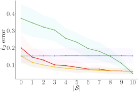
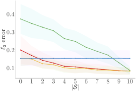
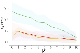
$M=20$

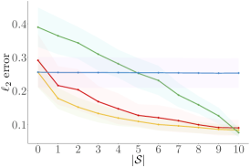
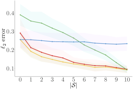
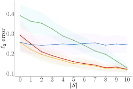
Figure 1: Simulation results for the $\ell_{2}$ errors. From left to right, results for the following values of $h$ are shown: 0.1, 1 and 3. The colored lines represent the mean $\ell_{2}$ error across 50 simulated datasets with $N_{s}=1000$ for respectively the following methods: Discovery BT , Oracle BT , Pooled BT and Primary attribute data only BT . The shaded area around the lines represent $\pm 1$ estimated standard deviation around the $\ell_{2}$ error.

	$M=10$		$M=20$
$S,N_{s},h$	Oracle BT/Discovery BT	BT/PBT	Oracle BT/Discovery BT	BT/PBT
$5,500,0.1$	0.14 (0.02)/0.17 (0.03)	0.22 (0.00)/0.26 (0.05)	0.22 (0.03)/0.29 (0.04)	0.37 (0.00)/0.30 (0.05)
$5,1000,0.1$	0.10 (0.01)/0.11 (0.02)	0.15 (0.00)/0.25 (0.05)	0.15 (0.02)/0.17 (0.03)	0.25 (0.00)/0.28 (0.05)
$5,1500,0.1$	0.08 (0.01)/0.09 (0.01)	0.12 (0.00)/0.25 (0.05)	0.13 (0.02)/0.13 (0.02)	0.20 (0.00)/0.27 (0.05)
$5,500,1$	0.16 (0.02)/0.19 (0.02)	0.22 (0.00)/0.27 (0.04)	0.23 (0.03)/0.29 (0.04)	0.37 (0.00)/0.31 (0.04)
$5,1000,1$	0.12 (0.01)/0.13 (0.01)	0.15 (0.00)/0.26 (0.04)	0.17 (0.02)/0.19 (0.02)	0.25 (0.00)/0.29 (0.04)
$5,1500,1$	0.10 (0.01)/0.11 (0.01)	0.12 (0.00)/0.26 (0.04)	0.14 (0.01)/0.15 (0.02)	0.20 (0.00)/0.28 (0.05)
$5,500,3$	0.20 (0.01)/0.22 (0.02)	0.22 (0.00)/0.30 (0.03)	0.25 (0.03)/0.30 (0.03)	0.36 (0.00)/0.32 (0.04)
$5,1000,3$	0.16 (0.01)/0.17 (0.01)	0.15 (0.00)/0.29 (0.03)	0.20 (0.02)/0.21 (0.02)	0.25 (0.00)/0.30 (0.04)
$5,1500,3$	0.14 (0.01)/0.14 (0.01)	0.12 (0.00)/0.29 (0.03)	0.17 (0.01)/0.17 (0.01)	0.20 (0.00)/0.30 (0.04)
$10,500,0.1$	0.11 (0.01)/0.15 (0.02)	0.24 (0.00)/0.24 (0.03)	0.17 (0.02)/0.25 (0.02)	0.37 (0.00)/0.26 (0.03)
$10,1000,0.1$	0.09 (0.01)/0.10 (0.01)	0.15 (0.00)/0.23 (0.03)	0.13 (0.02)/0.15 (0.02)	0.25 (0.00)/0.25 (0.03)
$10,1500,0.1$	0.07 (0.01)/0.08 (0.01)	0.12 (0.00)/0.23 (0.03)	0.10 (0.01)/0.11 (0.01)	0.23 (0.00)/0.24 (0.03)
$10,500,1$	0.14 (0.01)/0.16 (0.02)	0.24 (0.00)/0.24 (0.03)	0.19 (0.02)/0.25 (0.02)	0.36 (0.00)/0.26 (0.03)
$10,1000,1$	0.11 (0.01)/0.12 (0.01)	0.15 (0.00)/0.24 (0.03)	0.14 (0.01)/0.15 (0.02)	0.24 (0.00)/0.25 (0.03)
$10,1500,1$	0.09 (0.01)/0.10 (0.01)	0.12 (0.00)/0.24 (0.03)	0.12 (0.01)/0.12 (0.01)	0.19 (0.00)/0.25 (0.03)
$10,500,3$	0.18 (0.01)/0.20 (0.01)	0.23 (0.00)/0.27 (0.02)	0.21 (0.02)/0.25 (0.02)	0.36 (0.00)/0.28 (0.02)
$10,1000,3$	0.14 (0.00)/0.15 (0.00)	0.15 (0.00)/0.26 (0.02)	0.17 (0.01)/0.18 (0.02)	0.25 (0.00)/0.27 (0.03)
$10,1500,3$	0.13 (0.01)/0.13 (0.01)	0.12 (0.00)/0.26 (0.02)	0.15 (0.01)/0.15 (0.01)	0.20 (0.00)/0.26 (0.03)
$20,500,0.1$	0.09 (0.01)/0.13 (0.01)	0.24 (0.00)/0.23 (0.02)	0.14 (0.01)/0.23 (0.01)	0.36 (0.00)/0.24 (0.02)
$20,1000,0.1$	0.07 (0.01)/0.09 (0.01)	0.15 (0.00)/0.22 (0.02)	0.10 (0.01)/0.13 (0.01)	0.25 (0.00)/0.23 (0.02)
$20,1500,0.1$	0.06 (0.00)/0.07 (0.01)	0.12 (0.00)/0.22 (0.02)	0.09 (0.01)/0.09 (0.01)	0.20 (0.00)/0.23 (0.02)
$20,500,1$	0.11 (0.01)/0.14 (0.01)	0.24 (0.00)/0.23 (0.02)	0.15 (0.01)/0.22 (0.01)	0.35 (0.00)/0.24 (0.02)
$20,1000,1$	0.09 (0.01)/0.10 (0.01)	0.15 (0.00)/0.23 (0.02)	0.11 (0.01)/0.13 (0.01)	0.24 (0.00)/0.23 (0.02)
$20,1500,1$	0.08 (0.00)/0.08 (0.01)	0.12 (0.00)/0.23 (0.02)	0.10 (0.01)/0.10 (0.01)	0.19 (0.00)/0.23 (0.02)
$20,500,3$	0.15 (0.01)/0.17 (0.01)	0.24 (0.00)/0.25 (0.01)	0.17 (0.01)/0.25 (0.01)	0.37 (0.00)/0.25 (0.02)
$20,1000,3$	0.13 (0.01)/0.14 (0.01)	0.15 (0.00)/0.25 (0.01)	0.14 (0.01)/0.15 (0.01)	0.25 (0.00)/0.25 (0.02)
$20,1500,3$	0.11 (0.00)/0.12 (0.00)	0.12 (0.00)/0.25 (0.01)	0.12 (0.01)/0.13 (0.01)	0.20 (0.00)/0.25 (0.02)

Table 1: Results for the fitted Bradley-Terry models on simulated data. The $\ell_{2}$ errors are averaged across 50 fitted models for each parameter combination and across all results for the number of informative secondary variables $|\mathcal{S}|$, where $0\leq|\mathcal{S}|\leq S,S\in\{5,10,20\}$ and rounded to two decimals. Standard errors are provided between parentheses. Bold values represent the best result for that particular parameter combination across the four approaches. Oracle BT and Discovery BT represent the proposed methods provided by Algorithms 1 and 2 respectively, whilst BT and PBT represent the primary attribute data only and pooled Bradley-Terry approaches respectively.

Both Figure 1 and Table 1 illustrate the performance of the proposed method compared to the existing Bradley-Terry method on multi-attribute preference data. In general, the proposed method outperforms its competitors under a variety of settings. Unsurprisingly, the more similar the informative secondary attributes are to the primary attribute, that is a smaller $h$, the better the performance of the proposed method. Judging by Figure 1, fitting the Bradley-Terry model on only the data pertaining to the primary attribute, or on all data pooled together, results in favourable performance, or equivalent performance to the propose method, only if either no or all secondary attributes are informative respectively. In all other cases, that is $0<|\mathcal{S}|<S$, the proposed method shows better performance, prohibiting a single exception: the top right plot in Figure 1, where $h=3$ and $M=10$. Under this specific scenario, fitting the Bradley-Terry model on the data pertaining to the primary attribute results in and equivalent or better performance compared to the proposed method for $|\mathcal{S}|\leq 4$. The reason behind this particular result is that setting $h=3$ causes $\bm{\alpha}^{*}$ and $\bm{u}^{(s)}$ to deviate substantially as both vectors only consist of 10 elements, which, in turn, results in very different pairwise comparison data between the primary and informative secondary attributes. To offset the large bias in the $\bm{u}^{(s)}$, the set of informative secondary attributes needs to be substantial. In addition, based on the $\ell_{2}$ errors averaged across all $0\leq|\mathcal{S}|\leq S$ shown in Table 1, the performance of the proposed method improves when $S$ and by extension $\mathcal{S}$ increases. Whilst the performance of the pooled Bradley-Terry model also improves, the performance of the Bradley-Terry model fitted on only the data pertaining to primary attribute does not. Nevertheless, the gain in performance from using the proposed method can be substantial. Whilst, in general, the performance of the oracle and discovery Bradley-Terry algorithms is very similar, they can differ substantially when $M=20$ and $N_{s}=500$. This is because for all $(j,l)\in\mathcal{E}_{s}$, for some $1\leq s\leq S$ and $(j,l)\not\in\mathcal{E}_{0}$, the discovery method has problems with selecting the proper informative set of secondary attributes, given that these observations containing edge $(j,l)$ cause a large discrepancy $|L(\hat{\bm{\alpha}}^{(s)})-L(\hat{\bm{\alpha}}^{(0)})|$.

5 Eba consumer preferences

Cassava (Manihot esculenta) is a popular source of carbohydrates in the tropics (Cock, 1982), especially in Africa. A typical method of consumption is to peel and boil the root. However, due to its short shelf life, alternative (processed) food products based on cassava have been developed. One such product is eba: a staple swallow from West Africa that is based on cassava flour (Awoyale et al., 2021). Given the popularity of this swallow, cassava breeding companies might be interested in selecting the most preferred cassava variety by eba consumers, in order to one up the competition and increase their profits.

In this application, we will analyse preference data found in Olaosebikan et al. (2023), in order to evaluate which cassava varieties are best suited for eba consumption, as judged by consumers. By means of the full breaking procedure, the partial rankings are turned into pairwise comparisons from a set of 13 objects (cassava varieties) across eight attributes: the overall preference of the consumer, the color, odour, firmness, stretchability, taste, smoothness and mouldability of the cassava, where each attribute consists of 1200 pairwise comparisons. Each observation consists of a pairwise comparison on a certain attribute of two eba samples prepared from two different cassava varieties. As the primary attribute, we select the overall preference of the consumer, whilst the remaining attribute are considered to be secondary. The data was collected by having individuals taste and compare eba cooked by experienced eba preparers across Cameroon and Nigeria. The pairwise comparision graph for the data is provided in Figure 2.

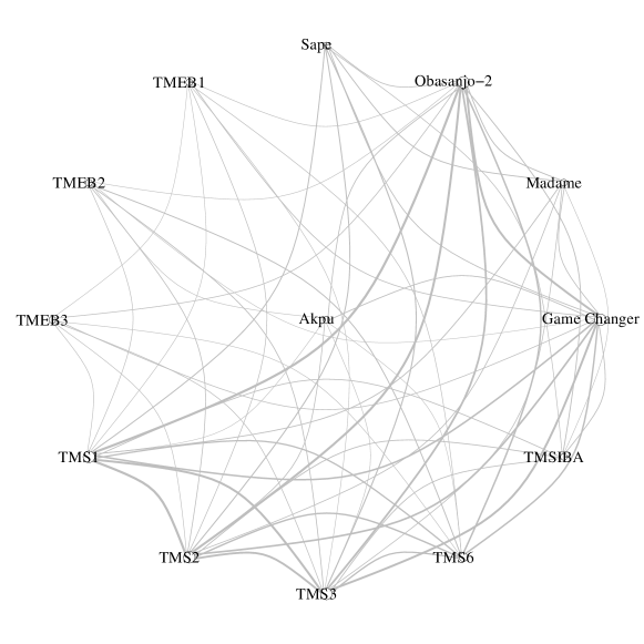
Figure 2: Pairwise comparision graph displaying which, and the number of times, objects are compared to each other on the primary attribute. Edges represent whether a pairwise comparison is present, and edge width represents the number of times a pairwise comparison is made.

From Figure 2, we note that the graph is not fully connected, implying that not all objects are directly compared with one another on the primary attribute, potentially resulting in worse parameter estimates, as is evident from Theorem 1. Nevertheless, the density of the graph, combined with the total number of observations should mitigate this problem to a large extend. We fit the proposed method (Algorithm 2) on the primary and secondary attribute data, as well as the Bradley-Terry model on the primary attribute data only. The proposed method assigns all secondary attributes to the informative set. Parameter estimates for both methods are provided in Table 2.

Table 2: Estimated worths and rankings using the proposed method for the cassava data.

	Discovery BT		Primary attribute only BT
Variety	Estimated worth	Estimated ranking	Estimated worth	Estimated ranking
Akpu	-0.67	13	-0.88	13
Game Changer	0.56	1	0.26	5
Madame	-0.03	8	0.37	3
Obasanjo-2	0.45	3	0.01	8
Sape	0.16	7	0.93	1
TMEB1	-0.49	10	0.27	4
TMEB2	-0.64	12	-0.64	12
TMEB3	-0.49	11	0.21	6
TMS1	0.30	5	-0.36	9
TMS2	0.21	6	-0.50	11
TMS3	0.48	2	0.05	7
TMS6	0.34	4	0.71	2
TMSIBA	-0.20	9	-0.42	10

Despite the similarity in some of the estimated parameters across the two methods, as well as the estimated rankings, in particular the worst ranked objects, many differences between the results from the proposed and the Bradley-Terry methods can be observed. Consider, for example, the top 3 ranking objects as per the proposed method: Game Changer, TMS3 and Obasanjo-2, none of which appear in the top 4 ranking objects of the Bradley-Terry method. Another notable result is that popular local and regional variaties such as Akpu, TMEB1, TMEB2 and TMEB3 are the worst ranked objects in terms of overall preference, raising the question as to why they are seen as popular varieties (Olaosebikan et al.,2023). Nevertheless, as all secondary attributes were assessed to be informative, such discrepancies were to be expected, given the simulation study results shown in Section 4.

6 Conclusion

In this contribution, we introduce a novel statistical method that is applicable to multi-attribute preference data, where the main interest lies in one of the various attributes: the primary attribute. Introducing the transfer learning framework to the Bradley-Terry model for pairwise comparison data, the proposed method outperforms existing methods both theoretically and empirically in a myriad of situations under which data is simulated. We apply the novel method on consumer preference data, although its applicability extends far beyond this particular example, as multi-attribute preference data is becoming more ubiquitous.

Even though the Bradley-Terry model provides a general framework for pairwise comparison data, the Plackett-Luce model is even more general, as it goes beyond pairwise comparisons by allowing for (partial) ranking data. Whilst the proposed framework has been shown to work under the Plackett-Luce model, no theoretical results are shown. This is largely due to the lack of statistical theory for the Plackett-Luce model, even for single-attribute preference data, which could be a direction for future research. In addition, the inclusion of features containing information about the individuals expressing their preferences or about the objects under consideration could provide to be a useful research endeavour, as this type of model can recommend objects to (new) individuals and predict the ranking of new objects. Whilst a bilinear model can accommodate for both these aims (Schäfer & Hüllermeier, 2018), it suffers from computational issues given that it has to estimate a large weight matrix consisting of each user-object feature combination. Therefore, implementing a computationally efficient bilinear model into the proposed framework is a second recommendation for future research.

Supplementary material

Appendix A Extension to partial ranking data

Even though this paper focuses on pairwise comparison data, the proposed method can easily be extended to (partial) ranking data, by using the likelihood of the Plackett-Luce model; a generalization of the Bradley-Terry model to (partial) rankings. Suppose that each individual provides a ranking across $2\leq m\leq M$ objects, then under the assumption that the worths follow a Plackett-Luce model, the probability of observing ranking $\bm{\pi}_{i}$, where $\bm{\pi}_{i}=\left\{\pi_{i1},\ldots,\pi_{im}\right\}$, $1\leq i\leq n,$ are permutations of $1,\ldots,m$, such that $\pi_{ij}$ denotes the rank of object $j$ according to ranker $i$, is given by

$$\mathbb{P}\left(\bm{\pi}_{i}|\bm{\alpha}\right)=\prod_{j=1}^{m}\frac{\exp(\alpha_{\sigma_{ij}})}{\sum_{l=j}^{m}\exp(\alpha_{\sigma_{il}})},$$

where $\alpha_{\sigma_{ij}}>0$ denotes the worth of the object ranked $j$-th by ranker $i$, and $\bm{\sigma}_{i}=\bm{\pi}^{-1}_{i}=\left\{\sigma_{i1},\ldots,\sigma_{im}\right\}$, where $\sigma_{ij}$ indicates the object ranked $j$-th by ranker $i$. Consequently, we obtain the following negative log likelihood

$$L(\bm{\alpha})=\sum_{i=1}^{n}\sum_{j=1}^{m}\left\{\log\left[\sum_{l=j}^{m}\exp(\alpha_{\sigma_{il}})\right]-\alpha_{\sigma_{ij}}\right\}.$$ (3)

By replacing the likelihood in Algorithms 1 and 2 in the main portion of this article with Equation (3), the proposed method can handle (partial) ranking data.

To illustrate the absolute and comparative effectiveness in parameter estimation of the proposed method, we simulate data in the same manner as in Section 4 of the main article, but instead sample partial rankings consisting of $m=3$ objects for each ranker, instead of pairwise comparisons. The results for these simulations are shown in Table 3.

	$M=10$		$M=20$
$S,N_{s},h$	Oracle PL/Discovery PL	PL/PPL	Oracle PL/Discovery PL	PL/PPL
$5,500,0.1$	0.09 (0.01)/0.10 (0.02)	0.14 (0.00)/0.25 (0.05)	0.14 (0.02)/0.15 (0.02)	0.22 (0.00)/0.27 (0.05)
$5,1000,0.1$	0.07 (0.01)/0.08 (0.01)	0.10 (0.00)/0.24 (0.05)	0.10 (0.01)/0.10 (0.01)	0.15 (0.00)/0.27 (0.05)
$5,1500,0.1$	0.06 (0.00)/0.06 (0.00)	0.08 (0.00)/0.24 (0.05)	0.09 (0.01)/0.09 (0.01)	0.12 (0.00)/0.26 (0.06)
$5,500,1$	0.11 (0.01)/0.12 (0.01)	0.14 (0.00)/0.26 (0.04)	0.15 (0.00)/0.16 (0.00)	0.22 (0.00)/0.29 (0.05)
$5,1000,1$	0.09 (0.00)/0.09 (0.01)	0.10 (0.00)/0.26 (0.05)	0.11 (0.01)/0.12 (0.01)	0.15 (0.00)/0.28 (0.05)
$5,1500,1$	0.07 (0.00)/0.08 (0.00)	0.08 (0.00)/0.26 (0.05)	0.10 (0.01)/0.10 (0.01)	0.12 (0.00)/0.28 (0.05)
$5,500,3$	0.15 (0.01)/0.16 (0.01)	0.14 (0.00)/0.29 (0.03)	0.18 (0.01)/0.19 (0.02)	0.22 (0.00)/0.30 (0.04)
$5,1000,3$	0.11 (0.01)/0.12 (0.00)	0.10 (0.00)/0.28 (0.03)	0.14 (0.01)/0.15 (0.01)	0.15 (0.00)/0.29 (0.04)
$5,1500,3$	0.10 (0.01)/0.09 (0.00)	0.08 (0.00)/0.28 (0.03)	0.12 (0.00)/0.12 (0.00)	0.12 (0.00)/0.29 (0.04)
$10,500,0.1$	0.08 (0.01)/0.09 (0.01)	0.14 (0.00)/0.23 (0.03)	0.11 (0.01)/0.13 (0.01)	0.21 (0.00)/0.25 (0.03)
$10,1000,0.1$	0.07 (0.00)/0.07 (0.01)	0.10 (0.00)/0.23 (0.03)	0.09 (0.01)/0.09 (0.01)	0.15 (0.00)/0.24 (0.03)
$10,1500,0.1$	0.06 (0.00)/0.06 (0.00)	0.08 (0.00)/0.23 (0.03)	0.08 (0.01)/0.08 (0.01)	0.12 (0.00)/0.24 (0.03)
$10,500,1$	0.10 (0.01)/0.11 (0.01)	0.14 (0.00)/0.24 (0.03)	0.12 (0.01)/0.14 (0.01)	0.22 (0.00)/0.25 (0.03)
$10,1000,1$	0.08 (0.00)/0.08 (0.00)	0.10 (0.00)/0.24 (0.03)	0.10 (0.01)/0.10 (0.01)	0.15 (0.00)/0.25 (0.03)
$10,1500,1$	0.07 (0.00)/0.07 (0.00)	0.08 (0.00)/0.24 (0.03)	0.09 (0.01)/0.09 (0.01)	0.12 (0.00)/0.25 (0.03)
$10,500,3$	0.13 (0.01)/0.14 (0.01)	0.14 (0.00)/0.27 (0.02)	0.15 (0.01)/0.16 (0.01)	0.22 (0.00)/0.27 (0.03)
$10,1000,3$	0.11 (0.00)/0.11 (0.00)	0.10 (0.00)/0.26 (0.02)	0.12 (0.01)/0.13 (0.01)	0.15 (0.00)/0.26 (0.03)
$10,1500,3$	0.09 (0.00)/0.09 (0.00)	0.08 (0.00)/0.26 (0.02)	0.11 (0.01)/0.12 (0.00)	0.12 (0.00)/0.26 (0.03)
$20,500,0.1$	0.07 (0.00)/0.08 (0.01)	0.14 (0.00)/0.22 (0.02)	0.09 (0.01)/0.11 (0.01)	0.22 (0.00)/0.23 (0.02)
$20,1000,0.1$	0.06 (0.00)/0.06 (0.00)	0.10 (0.00)/0.22 (0.02)	0.07 (0.01)/0.08 (0.01)	0.15 (0.00)/0.22 (0.02)
$20,1500,0.1$	0.05 (0.00)/0.05 (0.00)	0.08 (0.00)/0.21 (0.02)	0.07 (0.00)/0.07 (0.00)	0.13 (0.00)/0.22 (0.02)
$20,500,1$	0.08 (0.01)/0.09 (0.01)	0.00 (0.14)/0.23 (0.02)	0.10 (0.01)/0.11 (0.01)	0.22 (0.00)/0.23 (0.02)
$20,1000,1$	0.07 (0.00)/0.07 (0.00)	0.10 (0.00)/0.23 (0.02)	0.08 (0.01)/0.08 (0.01)	0.15 (0.00)/0.23 (0.02)
$20,1500,1$	0.06 (0.00)/0.06 (0.00)	0.08 (0.00)/0.23 (0.02)	0.08 (0.00)/0.08 (0.00)	0.12 (0.00)/0.23 (0.02)
$20,500,3$	0.12 (0.00)/0.13 (0.00)	0.14 (0.00)/0.25 (0.02)	0.13 (0.01)/0.14 (0.01)	0.22 (0.00)/0.25 (0.02)
$20,1000,3$	0.10 (0.00)/0.11 (0.00)	0.10 (0.00)/0.25 (0.02)	0.11 (0.01)/0.11 (0.01)	0.15 (0.00)/0.24 (0.02)
$20,1500,3$	0.08 (0.00)/0.09 (0.00)	0.08 (0.00)/0.25 (0.02)	0.09 (0.00)/0.10 (0.00)	0.12 (0.00)/0.24 (0.02)

Table 3: Results for the fitted Plackett-Luce models on simulated data. The $\ell_{2}$ errors are averaged across 50 fitted models for each parameter combination and across all results for the number of informative secondary variables $|\mathcal{S}|$, where $0\leq|\mathcal{S}|\leq S,S\in\{5,10,20\}$ and rounded to two decimals. Standard errors are provided between parentheses. Bold values represent the best result for that particular parameter combination across the four approaches. Oracle PL and Discovery PL represent the proposed methods provided by Algorithms 1 and 2, extended to partial ranking data, respectively, whilst PL and PPL represent the primary attribute data only and pooled Plackett-Luce approaches respectively.

Appendix B Proofs

Here we provide a proof of the main theoretical result of this paper, that is, Theorem 1 and Corollary 1. The proof borrows heavily from the proofs presented in Chen et al. (2019) and Fan et al. (2022).

To show that

$$||\hat{\bm{\alpha}}-\bm{\alpha}^{*}||_{\infty}\lesssim\kappa_{1}^{2}\sqrt{\frac{\log M}{Mp(n_{0}+n_{\mathcal{S}})}}+\kappa_{2}^{2}\sqrt{\frac{\log M}{Mpn_{0}}},$$

we use that

$$\begin{gathered}||\hat{\bm{\alpha}}-\bm{\alpha}^{*}||_{\infty}=||(\hat{\bm{u}}+\hat{\bm{\delta}}_{\lambda_{\delta}})-(\bm{u}^{*}+\bm{\delta}^{*})||_{\infty}\\ \leq||\hat{\bm{u}}-\bm{u}^{*}||_{\infty}+||\hat{\bm{\delta}}_{\lambda_{\delta}}-\bm{\delta}^{*}||_{\infty}\\ \lesssim\kappa_{1}^{2}\sqrt{\frac{\log M}{Mp(n_{0}+n_{\mathcal{S}})}}+\kappa_{2}^{2}\sqrt{\frac{\log M}{Mpn_{0}}},\end{gathered}$$

where we use the subscript $\lambda_{\delta}$ to denote the penalized estimate, and where the first inequality follows from the definition of $\hat{\bm{\alpha}}$ and $\bm{\alpha}^{*}$ and the second from the triangle inequality. The proof consists of obtaining the rates for $||\hat{\bm{u}}-\bm{u}^{*}||_{\infty}$ and $||\hat{\bm{\delta}}_{\lambda_{\delta}}-\bm{\delta}^{*}||_{\infty}$ and combining them. Proofs for both convergence rates are provided in Sections B.1 and B.3 respectively.

Before moving on to proving each of the respective bounds on $\hat{\bm{u}}$ and $\hat{\bm{\delta}}_{\lambda_{\delta}}$, we first provide two general results that apply to both the comparison graphs used in these proofs $\mathcal{G}_{0\cup\mathcal{S}}$ and $\mathcal{G}_{0}$, as the number of objects and the edge probability are the same for both graphs.

Lemma 1.

Suppose the pairwise comparison graph is an Erdős-Rényi random graph. Let $d_{i}$ be the degree of node $i$, $d_{\min}=\min_{1\leq i\leq M}d_{i}$ and $d_{\max}=\max{1\leq i\leq M}d_{i}$. If $Mp>c_{p}\log M$ for some sufficiently large constant $c_{p}>0$, then the following event

$$E_{0}=\left\{\frac{Mp}{2}\leq d_{\min}\leq d_{\max}\leq\frac{3Mp}{2}\right\}$$

occurs with probability exceeding $1-O(M^{-10})$.

Proof.

The proof follows from the Chernoff bound (c.f. Chen et al., 2019) ∎

In order to analyse the Hessian of the negative log likelihood functions, we require the Laplacian matrix (c.f. Chen et al., 2019; Fan et al., 2022); $\bm{L}_{\mathcal{G}}=\sum_{(j,l\in\mathcal{E},j>l)}(\bm{e}_{j}-\bm{e}_{l})(\bm{e}_{j}-\bm{e}_{l})^{T}$, where $\bm{e}_{1},\ldots,\bm{e}_{M}$ are the canonical basis vectors in $\mathbb{R}^{M}$. The following lemma provides bounds on the eigenvalues of this matrix

Lemma 2.

Suppose $Mp>c_{p}\log M$ for some sufficiently large constant $c_{p}>0$, then, the following event

$$E_{1}=\left\{\frac{Mp}{2}\leq\lambda_{\min,\perp}(\bm{L}_{\mathcal{G}})\leq||\bm{L}_{\mathcal{G}}||\leq 2Mp\right\}$$

occurs with probability exceeding $1-O(M^{-10})$ for for large $M$.

Proof.

The inequality $\frac{Mp}{2}\leq\lambda_{\min,\perp}(\bm{L}_{\mathcal{G}})$ follows from the fact that $\lambda_{\min,\perp}(\bm{L}_{\mathcal{G}})$ is the spectral gap of the Laplacian matrix, where the derivation is given by Tropp (2015). By definition, we know that $\lambda_{\min,\perp}(\bm{L}_{\mathcal{G}})\leq||\bm{L}_{\mathcal{G}}||$, but also that $||\bm{L}_{\mathcal{G}}||\leq d_{\max}\leq 2Mp$, completing the proof. ∎

B.1 Transfer convergence

Directly analysing the rate of $\hat{\bm{u}}$ is anything but straightforward. Instead, we first obtain the rate for the $\ell_{2}$ regularized version of $\bm{u}$, and show that the same rate holds for $\hat{\bm{u}}$, based on an appropriate value of $\lambda_{u}$. The regularization of the loss function guarantees a smooth and strongly convex optimization problem, which has the desirable property of a known fast rate of convergence for gradient descent algorithms (Bubeck, 2015).

Theorem 3.

Suppose $Mp>c_{p}\log M$ and $n_{0}+n_{\mathcal{S}}\leq c_{2}M^{c_{3}}$ for some $c_{p},c_{2},c_{3}>0$. In addition, we set $\lambda_{u}=c_{\lambda_{u}}\frac{1}{\log\kappa_{1}}\sqrt{\frac{Mp\log M}{n_{0}+n_{\mathcal{S}}}}$ for some $c_{\lambda_{u}}>0$. Then with probability exceeding $1-O(M^{-5})$ we have that

$$||\hat{\bm{u}}_{\lambda_{u}}-\bm{u}^{*}||_{\infty}\lesssim\kappa_{1}^{2}\sqrt{\frac{\log M}{Mp(n_{0}+n_{\mathcal{S}})}},$$

where $\hat{\bm{u}}_{\lambda_{u}}=\operatorname*{arg\,min}_{\bm{u}\in\mathbb{R}^{d}}L_{\lambda_{u}}(\bm{u})$, $L_{\lambda_{u}}(\bm{u})=L(\bm{u})+\frac{\lambda_{u}}{2}||\bm{u}||_{2}^{2}$.

Central in establishing Theorem 3 are the gradient and Hessian of $L_{\lambda_{u}}(\bm{u})$, an event that bounds the gradient and events that bound the eigenvalues of the gradient and Hessian. To this end, the gradient of $L_{\lambda_{u}}(\bm{u})$ is given by

$$\nabla L_{\lambda_{u}}(\bm{u})=\sum_{(j,l)\in\mathcal{E}_{0\cup\mathcal{S}},j>l}\left\{-y_{l,j}+\frac{\exp(u_{j})}{\exp(u_{j})+\exp(u_{l})}\right\}(\bm{e}_{j}-\bm{e}_{l})+\lambda_{u}\bm{u}$$

$$=\frac{1}{n_{0}+n_{\mathcal{S}}}\sum_{(j,l)\in\mathcal{E}_{0\cup\mathcal{S}},j>l}\sum_{i=1}^{n_{0}+n_{\mathcal{S}}}\left\{-y_{l,j}^{(i)}+\frac{\exp(u_{j})}{\exp(u_{j})+\exp(u_{l})}\right\}(\bm{e}_{j}-\bm{e}_{l})+\lambda_{u}\bm{u},$$ (4)

whilst the Hessian of $L_{\lambda_{u}}(\bm{u})$ is given by

$$\nabla^{2}L_{\lambda_{u}}(\bm{u})=\sum_{(j,l)\in\mathcal{E}_{0\cup\mathcal{S}},j>l}\left\{-y_{l,j}+\frac{\exp(u_{j}+u_{l})}{[\exp(u_{j})+\exp(u_{l})]^{2}}\right\}(\bm{e}_{j}-\bm{e}_{l})(\bm{e}_{j}-\bm{e}_{l})^{T}+\lambda_{u}$$

$$=\frac{1}{n_{0}+n_{\mathcal{S}}}\sum_{(j,l)\in\mathcal{E}_{0\cup\mathcal{S}},j>l}\sum_{i=1}^{n_{0}+n_{\mathcal{S}}}\left\{-y_{l,j}^{(i)}+\frac{\exp(u_{j}+u_{l})}{[\exp(u_{j})+\exp(u_{l})]^{2}}\right\}(\bm{e}_{j}-\bm{e}_{l})(\bm{e}_{j}-\bm{e}_{l})^{T}+\lambda_{u},$$ (5)

where we denote $\left\{-y_{l,j}^{(i)}+\frac{\exp(u_{j}^{*})}{\exp(u_{j}^{*})+\exp(u_{l}^{*})}\right\}(\bm{e}_{j}-\bm{e}_{l})$ as $z_{j,l}^{(i)}$.

The next three Lemmas provide bounds on the values of the gradient, as well as bounds on the eigenvalues of the gradient and Hessian and are used intensively throughout this proof.

Lemma 3.

For $\lambda_{u}=c_{\lambda_{u}}\frac{1}{\log\kappa_{1}}\sqrt{\frac{Mp\log M}{n_{0}+n_{\mathcal{S}}}}$, the following event

$$E_{2}=\left\{||\nabla L_{\lambda_{u}}(\bm{u}^{*})||_{2}\leq c_{0}\sqrt{\frac{M^{2}p\log M}{n_{0}+n_{\mathcal{S}}}}\right\}$$

is obtained with probability exceeding $1-O(M^{-10})$ for $c_{0}>0$, where $c_{0}$ depends on $c_{\lambda_{u}}$.

Proof.

Since $\mathbb{E}[z_{j,l}^{(i)}]=0,||z_{j,l}^{(i)}||_{2}\leq||\bm{e}_{j}-\bm{e}_{l}||_{2}\leq\sqrt{2}$ we have that

$$\mathbb{E}[z_{j,l}^{(i)}z_{j,l}^{(i)T}]=\text{Var}[y_{l,j}^{(i)}](\bm{e}_{j}-\bm{e}_{l})(\bm{e}_{j}-\bm{e}_{l})^{T}\prec(\bm{e}_{j}-\bm{e}_{l})(\bm{e}_{j}-\bm{e}_{l})^{T}$$

and

$$\mathbb{E}[z_{j,l}^{(i)T}z_{j,l}^{(i)}]\leq 2.$$

Thus, with high probability, we have that

$$\left|\left|\sum_{(j,l)\in\mathcal{E}_{0\cup\mathcal{S}},j>l}\sum_{i=1}^{n_{0}+n_{\mathcal{S}}}\mathbb{E}[z_{j,l}^{(i)}z_{j,l}^{(i)T}]\right|\right|\leq(n_{0}+n_{\mathcal{S}})\left|\left|\sum_{(j,l)\in\mathcal{E}_{0\cup\mathcal{S}},j>l}(\bm{e}_{j}-\bm{e}_{l})(\bm{e}_{j}-\bm{e}_{l})^{T}\right|\right|\lesssim(n_{0}+n_{\mathcal{S}})Mp$$

and

$$\left|\left|\sum_{(j,l)\in\mathcal{E}_{0\cup\mathcal{S}},j>l}\sum_{i=1}^{n_{0}+n_{\mathcal{S}}}\mathbb{E}[z_{j,l}^{(i)T}z_{j,l}^{(i)}]\right|\right|\leq 2(n_{0}+n_{\mathcal{S}})\left|\sum_{(j,l)\in\mathcal{E}_{0\cup\mathcal{S}},j>l}1\right|\lesssim(n_{0}+n_{\mathcal{S}})M^{2}p.$$

Let $V=\frac{1}{(n_{0}+n_{\mathcal{S}})^{2}}\max\left\{\left|\left|\sum_{(j,l)\in\mathcal{E}_{0\cup\mathcal{S}},j>l}\sum_{i=1}^{n_{0}+n_{\mathcal{S}}}\mathbb{E}[z_{j,l}^{(i)}z_{j,l}^{(i)T}]\right|\right|,\left|\sum_{(j,l)\in\mathcal{E}_{0\cup\mathcal{S}},j>l}\sum_{i=1}^{n_{0}+n_{\mathcal{S}}}\mathbb{E}[z_{j,l}^{(i)T}z_{j,l}^{(i)}]\right|\right\}$ and $B=\max_{i,j,l}||z_{j,l}^{(i)}||/(n_{0}+n_{\mathcal{S}})$. By applying the matrix Bernstein inequality, we have that

$$\begin{gathered}\left|\left|\nabla L_{\lambda_{u}}(\bm{u}^{*})-\mathbb{E}\left[\nabla L_{\lambda_{u}}(\bm{u}^{*})|\mathcal{G}_{0\cup\mathcal{S}}\right]\right|\right|_{2}\lesssim\sqrt{V\log M}+B\log M\lesssim\sqrt{\frac{M^{2}p\log M}{n_{0}+n_{\mathcal{S}}}}+\frac{\log M}{n_{0}+n_{\mathcal{S}}}\\ \lesssim\sqrt{\frac{M^{2}p\log M}{n_{0}+n_{\mathcal{S}}}},\end{gathered}$$

with probability exceeding $1-O(M^{-10})$. In addition, given that $\left|\left|\mathbb{E}\left[\nabla L_{\lambda_{u}}(\bm{u}^{*})|\mathcal{G}_{0\cup\mathcal{S}}\right]\right|\right|_{2}=\lambda_{u}\bm{u}^{*}$, we have that

$$\begin{gathered}\left|\left|\left[\nabla L_{\lambda_{u}}(\bm{u}^{*})\right]\right|\right|_{2}\leq\left|\left|\mathbb{E}\left[\nabla L_{\lambda_{u}}(\bm{u}^{*})|\mathcal{G}_{0\cup\mathcal{S}}\right]\right|\right|_{2}+||\left[\nabla L_{\lambda_{u}}(\bm{u}^{*})\right]-\mathbb{E}\left[\nabla L_{\lambda_{u}}(\bm{u}^{*})|\mathcal{G}_{0\cup\mathcal{S}}\right]||_{2}\\ \lesssim\lambda_{u}||\bm{u}^{*}||_{2}+\sqrt{\frac{M^{2}p\log M}{n_{0}+n_{\mathcal{S}}}}\asymp\sqrt{\frac{M^{2}p\log M}{n_{0}+n_{\mathcal{S}}}}\end{gathered}$$

with high probability. This relationship holds, as $||\bm{u}^{*}||_{2}\leq\sqrt{M}\log\kappa_{1}$, $\lambda\asymp\frac{1}{\log\kappa_{1}}\sqrt{\frac{Mp\log M}{n_{0}+n_{\mathcal{S}}}}$, and

$$\lambda_{u}||\bm{u}^{*}||_{2}\lesssim\frac{\sqrt{M}\log\kappa_{1}}{\log\kappa_{1}}\sqrt{\frac{Mp\log M}{n_{0}+n_{\mathcal{S}}}}\lesssim\sqrt{\frac{M^{2}p\log M}{n_{0}+n_{\mathcal{S}}}},$$

Giving us the desired result that

$$||\nabla L_{\lambda_{u}}(\bm{u}^{*})||_{2}\leq c_{0}\sqrt{\frac{M^{2}p\log M}{n_{0}+n_{\mathcal{S}}}},$$

for some $c_{0}>0$. ∎

Without loss of generality, for the remainder of the results, we assume the conditions stated in Lemma 3 hold.

Lemma 4.

Suppose $E_{1}$ (see Lemma 2) happens. Then, we have that

$$\lambda_{\max}(\nabla^{2}L_{\lambda_{u}}(\bm{u}))\leq\lambda_{u}+Mp,\quad\forall\bm{u}\in\mathbb{R}^{M}\text{ s.t. }\bm{1}_{M}\bm{u}=0.$$

Proof.

As $\frac{\exp(u_{j}+u_{l})}{[\exp(u_{j})+\exp(u_{l})]^{2}}\leq 0.25$, we have that

$$\lambda_{\max}(\nabla^{2}L_{\lambda_{u}}(\bm{u}))\leq\lambda_{u}+\frac{1}{2}||\bm{L}_{\mathcal{G}_{0\cup\mathcal{S}}}||\leq\lambda_{u}+Mp,\quad\forall\bm{u}\in\mathbb{R}^{M}\text{ s.t. }\bm{1}_{M}\bm{u}=0.$$

∎

Lemma 5.

Suppose $E_{1}$ (see Lemma 2) happens. Then, for all $||\bm{u}-\bm{u}^{*}||_{2}\leq c_{1}$ we have that

$$\lambda_{\min,\perp}(\nabla^{2}L_{\lambda_{u}}(\bm{u}))\geq\lambda_{u}+\frac{Mp}{8\kappa_{1}\exp(2c_{1})}$$

Proof.

Without loss of generality, for any $1\leq j\neq l\leq M$, we assume that $u_{j}\leq u_{l}$. Consequently, we have that

$$\frac{\exp(u_{j}+u_{l})}{[\exp(u_{j})+\exp(u_{l})]^{2}}=\frac{\exp[u_{j}-u_{l}]}{\{1+\exp[u_{j}-u_{l}]\}^{2}}=\frac{\exp[-|u_{j}-u_{l}|]}{\{1+\exp[-|u_{j}-u_{l}|]\}^{2}}\geq\frac{1}{4}\exp[-|u_{j}-u_{l}|].$$

Moreover, we have that

$$\begin{gathered}|u_{j}-u_{l}|=|(u_{j}-u_{l})+(u_{j}^{*}-u_{j}^{*})+(u_{l}^{*}-u_{l}^{*})|\\ \leq|u_{j}^{*}-u_{l}^{*}|+|u_{j}^{*}-u_{j}|+|u_{l}^{*}-u_{l}|\\ \leq\log(\kappa_{1})+2c_{1}\end{gathered}$$

As such, we have that

$$\frac{\exp(u_{j}+u_{l})}{[\exp(u_{j})+\exp(u_{l})]^{2}}\geq\frac{1}{4\kappa_{1}\exp(2c_{1})}$$

This gives us the following bound for the eigenvalues of the Hessian

$$\lambda_{\min,\perp}(\nabla^{2}L_{\lambda_{u}}(\bm{u}))\geq\lambda_{u}+\frac{1}{4\kappa_{1}\exp(2c_{1})}\lambda_{\min,\perp}(\bm{L}_{\mathcal{G}_{0\cup\mathcal{S}}})\geq\lambda_{u}+\frac{Mp}{8\kappa_{1}\exp(2c_{1})}$$

∎

B.1.1 Gradient Descent

Parameter estimation is conducted using the projected gradient descent algorithm. As such, a sequence of estimates $\{\bm{u}^{t}\}_{t=0,1,\ldots}$ is generated, where the step size $\eta$ is set at $\frac{1}{\lambda_{u}+Mp}$ and the number of iterations $T=M^{5}$.

Algorithm 3 Gradient descent for regularized MLE

1:  Initialise $\bm{u}^{[0]}=\bm{u}^{*}$

2:  for $t=0$ to $T-1$ do

3:     $\bm{u}^{[t+1]}=\bm{u}^{[t]}-\eta\nabla L_{\lambda_{u}}(\bm{u}^{[t]})$

4:  end for

Lemma 6.

Suppose $E_{0}$ (see Lemma 1) happens. Then, we have that

$$||\bm{u}^{[t]}-\hat{\bm{u}}_{\lambda_{u}}||_{2}\leq\rho^{[T]}||\bm{u}^{[t]}-\hat{\bm{u}}_{\lambda_{u}}||_{2},$$

where $\rho=1-\frac{\lambda_{u}}{\lambda_{u}+Mp}$.

Proof.

The convergence property of a smooth, strongly convex function ($L_{\lambda_{u}}(\cdot)$) is shown by Bubeck (2015). ∎

Lemma 7.

Suppose $E_{2}$ (see Lemma 3) happens. Then, we have that

$$||\bm{u}^{[0]}-\hat{\bm{u}}_{\lambda_{u}}||_{2}=||\hat{\bm{u}}_{\lambda_{u}}-\bm{u}^{*}||_{2}\leq c_{2}\log\kappa_{1}\sqrt{M}$$

where $\rho=1-\frac{\lambda_{u}}{\lambda_{u}+Mp}$.

Proof.

Since $\hat{\bm{u}}_{\lambda_{u}}$ is the minimizer, we have that $L_{\lambda_{u}}(\bm{u}^{*})\geq L_{\lambda_{u}}(\hat{\bm{u}}_{\lambda_{u}})$. By the mean value theorem, for some $\bm{u}^{\prime}$ between $\bm{u}^{*}$ and $\hat{\bm{u}}_{\lambda_{u}}$, we have

$$L_{\lambda_{u}}(\hat{\bm{u}}_{\lambda_{u}})=L_{\lambda_{u}}(\bm{u}^{*})+\nabla L_{\lambda_{u}}(\bm{u}^{*})^{T}(\hat{\bm{u}}_{\lambda_{u}}-\bm{u}^{*})+\frac{1}{2}(\hat{\bm{u}}_{\lambda_{u}}-\bm{u}^{*})^{T}\nabla^{2}L_{\lambda_{u}}(\bm{u}^{\prime})(\hat{\bm{u}}_{\lambda_{u}}-\bm{u}^{*}).$$

Consequently, we have that

$$\begin{gathered}L_{\lambda_{u}}(\bm{u}^{*})\geq L_{\lambda_{u}}(\bm{u}^{*})+\nabla L_{\lambda_{u}}(\bm{u}^{*})^{T}(\hat{\bm{u}}_{\lambda_{u}}-\bm{u}^{*})+\frac{1}{2}(\hat{\bm{u}}_{\lambda_{u}}-\bm{u}^{*})^{T}\nabla^{2}L_{\lambda_{u}}(\bm{u}^{*})(\hat{\bm{u}}_{\lambda_{u}}-\bm{u}^{*})\\ \geq L_{\lambda_{u}}(\bm{u}^{*})+\nabla L_{\lambda_{u}}(\bm{u}^{*})^{T}(\hat{\bm{u}}_{\lambda_{u}}-\bm{u}^{*})+\frac{\lambda_{u}}{2}||\hat{\bm{u}}_{\lambda_{u}}-\bm{u}^{*}||_{2}^{2}.\end{gathered}$$

Which results in

$$\begin{gathered}\frac{\lambda_{u}}{2}||\hat{\bm{u}}_{\lambda_{u}}-\bm{u}^{*}||_{2}^{2}\leq-\nabla L_{\lambda_{u}}(\bm{u}^{*})^{T}(\hat{\bm{u}}_{\lambda_{u}}-\bm{u}^{*})\\ \leq||\nabla L_{\lambda_{u}}(\bm{u}^{*})||_{2}||\hat{\bm{u}}_{\lambda_{u}}-\bm{u}^{*}||_{2}\end{gathered}$$

Finally, suppose $E_{2}$ happens. Then, we have that

$$||\hat{\bm{u}}_{\lambda_{u}}-\bm{u}^{*}||_{2}\leq\frac{2||\nabla L_{\lambda_{u}}(\bm{u}^{*})||_{2}}{\lambda_{u}}\leq\frac{2c_{0}\sqrt{\frac{M^{2}p\log M}{n_{0}+n_{\mathcal{S}}}}}{c_{\lambda_{u}}\frac{1}{\log\kappa_{1}}\sqrt{\frac{Mp\log M}{n_{0}+n_{\mathcal{S}}}}}\leq c_{2}\log\kappa_{1}\sqrt{M},$$

for $c_{2}\geq\frac{2c_{0}}{c_{\lambda_{u}}}$. ∎

Lemma 8.

Suppose both $E_{0}$ and $E_{2}$ happen. Then, there exists some constant $C_{0}$, such that

$$||\bm{u}^{[T]}-\hat{\bm{u}}_{\lambda_{u}}||_{\infty}\leq C_{0}\kappa_{1}^{2}\sqrt{\frac{\log M}{Mp(n_{0}+n_{\mathcal{S}})}}.$$

Proof.

$$\begin{gathered}||\bm{u}^{[T]}-\hat{\bm{u}}_{\lambda_{u}}||_{2}\leq\rho^{[T]}||\bm{u}^{[0]}-\hat{\bm{u}}_{\lambda_{u}}||_{2}\text{ {(Lemma \ref{lemma:lemma5_step1})}}\\ \leq\left(1-\frac{\lambda_{u}}{\lambda_{u}+Mp}\right)^{M^{5}}c_{2}\log\kappa_{1}\sqrt{M}\text{ {(Lemmas \ref{lemma:lemma5_step1} and \ref{lemma:lemma6_step1})}}\\ \leq c_{2}\exp\left(-\frac{\lambda_{u}M^{5}}{\lambda_{u}+Mp}\right)\kappa_{1}^{2}\sqrt{M}\\ \leq c_{2}\exp\left(-\frac{M^{5}}{c_{3}\log\kappa_{1}}\sqrt{\frac{\log M}{Mp(n_{0}+n_{\mathcal{S}})}}\right)\kappa_{1}^{2}\sqrt{M}\left(\text{By }Mp>\lambda_{u}\right)\\ \leq c_{2}\exp\left(-\frac{M^{5}}{c_{4}\log M}\sqrt{\frac{\log M}{Mp(n_{0}+n_{\mathcal{S}})}}\right)\kappa_{1}^{2}\sqrt{M}\left(\text{By }\kappa_{1}^{4}\lesssim\frac{Mp}{\log M}\lesssim\frac{M}{\log M}\right)\\ \leq C_{0}\kappa_{1}^{2}\sqrt{\frac{\log M}{Mp(n_{0}+n_{\mathcal{S}})}},\end{gathered}$$

for constants $C_{0},c_{2},c_{3}>0$ and $n_{0}+n_{\mathcal{S}}\lesssim M^{5}$. This gives the following bound

$$||\bm{u}^{[T]}-\hat{\bm{u}}_{\lambda_{u}}||_{\infty}\leq||\bm{u}^{[T]}-\hat{\bm{u}}_{\lambda_{u}}||_{2}\leq C_{0}\kappa_{1}^{2}\sqrt{\frac{\log M}{Mp(n_{0}+n_{\mathcal{S}})}}.$$

∎

B.2 Leave-one-out technique

Next, we concern ourselves with the statistical error of $\hat{\bm{u}}_{\lambda_{u}}$. This is done by using the leave-one-out technique (Ma et al., 2018; Chen et al., 2019, 2020), combined with a proof by induction to show that $\bm{u}^{[T]}$ does not deviate too strongly from $\bm{u}^{*}$, even after many iterations of Algorithm 3. We proceed by considering the following loss function for any $1\leq k\leq M$.

$$\begin{gathered}L^{(k)}(\bm{u})=\sum_{(j,l)\in\mathcal{E},j>l,j\neq k,l\leq q}\left\{-y_{l,j}\left(u_{j}-u_{l}\right)+\log\left[1+\exp(u_{j}-u_{l})\right]\right\}\\ +p\sum_{j\neq k}\left\{-\frac{\exp(u_{j}^{*})}{\exp(u_{j}^{*})+\exp(u_{k}^{*})}(u_{j}-u_{k})+\log\left[1+\exp(u_{j}-u_{k})\right]\right\}\\ L^{(k)}_{\lambda_{u}}(\bm{u})=L^{(k)}(\bm{u})+\frac{\lambda_{u}}{2}||\bm{u}||_{2}^{2}.\end{gathered}$$

Algorithm 4 then describes how the leave one out sequences $\{\bm{u}^{[t],(k)}\}_{t=0,1,\ldots}$ are constructed.

Algorithm 4 Leave-one-out sequence constructor.

1:  Initialise $\bm{u}^{[0],(k)}=\bm{u}^{*}$

2:  for $t=0$ to $T-1$ do

3:     $\bm{u}^{[t+1],(k)}=\bm{u}^{[t],(k)}-\eta\nabla L_{\lambda_{u}}^{(k)}(\bm{u}^{[t],(k)})$

4:  end for

Note that $\bm{u}^{[t],(k)}$ denotes iterate $t$ for the $k$-th leave-one-out sequence, and is a vector consisting of $M$ elements, whereas $u^{[t],(k)}_{k}$ is a scalar. Whilst the previous section was concerned with establishing the convergence of the gradient descent algorithm, that is, the iterates are close to the MLE, the aim here is to show that $\bm{u}^{[T]}$ is close to $\bm{u}^{*}$. The following bounds are proven by induction in Lemmas 10, 11, 12 and 13 respectively

$$||\bm{u}^{[t]}-\bm{u}^{*}||_{2}\leq C_{1}\kappa_{1}\sqrt{\frac{\log M}{p(n_{0}+n_{\mathcal{S}})}},$$ (6)

$$\max_{1\leq k\leq M}|u^{[t],(k)}_{k}-u_{k}^{*}|\leq C_{2}\kappa_{1}^{2}\sqrt{\frac{\log M}{Mp(n_{0}+n_{\mathcal{S}})}},$$ (7)

$$\max_{1\leq k\leq M}||\bm{u}^{[t]}-\bm{u}^{[t],(k)}||_{2}\leq C_{3}\kappa_{1}\sqrt{\frac{\log M}{Mp(n_{0}+n_{\mathcal{S}})}},$$ (8)

$$||\bm{u}^{[t]}-\bm{u}^{*}||_{\infty}\leq C_{4}\kappa_{1}^{2}\sqrt{\frac{\log M}{Mp(n_{0}+n_{\mathcal{S}})}}.$$ (9)

Lemma 9.

Suppose that the bounds provided in Equations 6-9 hold for iteration $t$. Then, there exists $C_{5},C_{6}>0$, such that

$$\max_{1\leq k\leq M}||\bm{u}^{[t],(k)}-\bm{u}^{*}||_{\infty}\leq C_{5}\kappa_{1}^{2}\sqrt{\frac{\log M}{Mp(n_{0}+n_{\mathcal{S}})}},$$ (10)

$$\max_{1\leq k\leq M}||\bm{u}^{[t],(k)}-\bm{u}^{*}||_{2}\leq C_{6}\kappa_{1}\sqrt{\frac{\log M}{p(n_{0}+n_{\mathcal{S}})}}.$$ (11)

Proof.

We begin by proving the first equation of this lemma:

$$\begin{gathered}\max_{1\leq k\leq M}||\bm{u}^{[t],(k)}-\bm{u}^{*}||_{\infty}\leq\max_{1\leq k\leq M}||\bm{u}^{[t]}-\bm{u}^{[t],(k)}||_{2}+||\bm{u}^{[t]}-\bm{u}^{*}||_{\infty}\text{ (Triangle inequality)}\\ \leq C_{3}\kappa_{1}\sqrt{\frac{\log M}{Mp(n_{0}+n_{\mathcal{S}})}}+C_{4}\kappa_{1}^{2}\sqrt{\frac{\log M}{Mp(n_{0}+n_{\mathcal{S}})}}\text{ (Equations \ref{eq:bound3_step1} and \ref{eq:bound4_step1})}\\ \leq C_{5}\kappa_{1}^{2}\sqrt{\frac{\log M}{Mp(n_{0}+n_{\mathcal{S}})}},\end{gathered}$$

provided that $C_{5}\leq C_{3}+C_{4}$. The second equation is proven by the fact that

$$\begin{gathered}\max_{1\leq k\leq M}||\bm{u}^{[t],(k)}-\bm{u}^{*}||_{2}\leq\max_{1\leq k\leq M}||\bm{u}^{[t]}-\bm{u}^{[t],(k)}||_{2}+||\bm{u}^{[t]}-\bm{u}^{*}||_{2}\text{ (Triangle inequality)}\\ \leq C_{3}\kappa_{1}\sqrt{\frac{\log M}{Mp(n_{0}+n_{\mathcal{S}})}}+C_{1}\kappa_{1}\sqrt{\frac{\log M}{p(n_{0}+n_{\mathcal{S}})}}\text{ (Equations \ref{eq:bound3_step1} and \ref{eq:bound1_step1})}\\ \leq C_{6}\kappa_{1}\sqrt{\frac{\log M}{p(n_{0}+n_{\mathcal{S}})}},\end{gathered}$$

provided that $C_{6}\leq C_{1}+C_{3}$. ∎

Lemma 10.

Suppose that the bounds provided in Equations 6-9 hold for iteration $t$. Then, with with probability exceeding $1-O(M^{-10})$ we have that

$$||\bm{u}^{[t+1]}-\bm{u}^{*}||_{2}\leq C_{1}\kappa_{1}\sqrt{\frac{\log M}{p(n_{0}+n_{\mathcal{S}})}}.$$

provided that $0<\eta\leq\frac{1}{\lambda_{u}+Mp}$ and $C_{1}$ is sufficiently large.

Proof.

We know (by definition) that

$$\begin{gathered}\bm{u}^{[t+1]}-\bm{u}^{*}=\bm{u}^{[t]}-\eta\nabla L_{\lambda_{u}}(\bm{u}^{[t]})-\bm{u}^{*}\\ =(\bm{u}^{[t]}-\bm{u}^{*})-[\eta\nabla L_{\lambda_{u}}(\bm{u}^{[t]})-\eta\nabla L_{\lambda_{u}}(\bm{u}^{*})]-\eta\nabla L_{\lambda_{u}}(\bm{u}^{*})\end{gathered}$$

Then, consider $\bm{u}(\tau)=\bm{u}^{*}+\tau\left(\bm{u}^{[t]}-\bm{u}^{*}\right)$. Using that the fundamental theorem of calculus gives $\nabla L_{\lambda_{u}}(\bm{u}^{[t]})-\nabla L_{\lambda_{u}}(\bm{u}^{*})=\int_{0}^{1}\nabla^{2}L_{\lambda_{u}}(\bm{u}(\tau))(\bm{u}^{[t]}-\bm{u}^{*})d\tau$, we obtain

$$\begin{gathered}(\bm{u}^{[t]}-\bm{u}^{*})-\eta[\nabla L_{\lambda_{u}}(\bm{u}^{[t]})-\nabla L_{\lambda_{u}}(\bm{u}^{*})]-\eta\nabla L_{\lambda_{u}}(\bm{u}^{*})\\ =\left(\bm{I}_{M}-\eta\int_{0}^{1}\nabla^{2}L_{\lambda_{u}}(\bm{u}(\tau))d\tau\right)\left(\bm{u}^{[t]}-\bm{u}^{*}\right)-\eta\nabla L_{\lambda_{u}}(\bm{u}^{*}).\end{gathered}$$

Now, let $u_{\max}(\tau):=\max_{j}u_{j}(\tau)$ and $u_{\min}(\tau):=\min_{j}u_{j}(\tau)$, then for $0\leq\tau\leq 1$ we have that

$$u_{\max}(\tau)-u_{\min}(\tau)\leq u_{\max}^{*}-u_{\min}^{*}+2||\bm{u}^{[t]}-\bm{u}^{*}||_{\infty}\leq\log\kappa_{1}+\epsilon,$$

for $\epsilon>0$, provided that $\epsilon\geq 2C_{4}\kappa_{1}^{2}\sqrt{\frac{\log M}{Mp(n_{0}+n_{\mathcal{S}})}}$, as obtained from the bound in Equation (9). Lemma 5 shows that for $0\leq\tau\leq 1$ we have that

$$\frac{Mp}{10\kappa_{1}}+\lambda_{u}\leq\frac{Mp}{8\kappa_{1}\exp(\epsilon)}+\lambda_{u}\leq\lambda_{\min,\perp}(\nabla^{2}L_{\lambda_{u}}(\bm{u}))\leq\lambda_{\max}(\nabla^{2}L_{\lambda_{u}}(\bm{u}))\leq\lambda_{u}+Mp$$

Now, let $\bm{A}=\int_{0}^{1}\nabla^{2}L_{\lambda_{u}}(\bm{u}(\tau))d\tau$, then we have that

$$\lambda_{u}+\frac{Mp}{10\kappa_{1}}\leq\lambda_{\min,\perp}\left(\bm{A}\right)\leq\lambda_{\max}\left(\bm{A}\right)\leq\lambda_{u}+Mp.$$

This gives the following upper bound

$$\begin{gathered}\left|\left|\left(\bm{I}_{d}-\eta\bm{A}\right)\left(\bm{u}^{[t]}-\bm{u}^{*}\right)\right|\right|_{2}\leq\max\{1-\lambda_{\min,\perp}\left(\bm{A}\right),1-\eta\lambda_{\max}\left(\bm{A}\right)\}\left|\left|\bm{u}^{[t]}-\bm{u}^{*}\right|\right|_{2}\\ \leq\left(1-\frac{\eta Mp}{10\kappa_{1}}\right)\left|\left|\bm{u}^{[t]}-\bm{u}^{*}\right|\right|_{2}\end{gathered}$$

Suppose $E_{1}$ happens. Then, by the triangle inequality we have that

$$\begin{gathered}\left|\left|\bm{u}^{[t+1]}-\bm{u}^{*}\right|\right|_{2}\leq\left|\left|\left(\bm{I}_{d}-\eta\bm{A}\right)\left(\bm{u}^{[t]}-\bm{u}^{*}\right)\right|\right|_{2}+\eta\left|\left|\nabla L_{\lambda_{u}}(\bm{u}^{*})\right|\right|_{2}\\ \leq\left(1-\frac{\eta Mp}{10\kappa_{1}}\right)C_{1}\kappa_{1}\sqrt{\frac{\log M}{p(n_{0}+n_{\mathcal{S}})}}+\eta c_{0}\sqrt{\frac{M^{2}p\log M}{(n_{0}+n_{\mathcal{S}})}}\text{ (Lemma \ref{lemma:lemma3_step1} and Equation (\ref{eq:bound1_step1}))}\\ \leq C_{1}\kappa_{1}\sqrt{\frac{\log M}{p(n_{0}+n_{\mathcal{S}})}},\end{gathered}$$

provided that $C_{1}>0$ is sufficiently large. ∎

Lemma 11.

Suppose that the bounds provided in Equations 6-9 hold for iteration $t$. Then, with probability exceeding $1-O(M^{-10})$ we have that

$$\max_{1\leq k\leq M}|u_{k}^{[t+1],(k)}-u_{k}^{*}|\leq C_{2}\kappa_{1}^{2}\sqrt{\frac{\log M}{Mp(n_{0}+n_{\mathcal{S}})}}$$

provided that $0<\eta\leq\frac{1}{\lambda_{u}+Mp}$ and $C_{2}\gtrsim C_{6}+c_{\lambda_{u}}$.

Proof.

The proof that the bound in above Equation holds depends on the leave one out algorithm defined in 4. The iterates of this algorithm are updated as follows

$$\bm{u}^{[t+1],(k)}=\bm{u}^{[t],(k)}-\eta\nabla L_{\lambda_{u}}^{(k)}(\bm{u}^{[t],(k)}).$$

This gives us that

$$u_{k}^{[t+1],(k)}-u_{k}^{*}=u_{k}^{[t],(k)}-\eta\left(\nabla L_{\lambda_{u}}^{(k)}(\bm{u}^{[t],(k)})\right)_{k}-u_{k}^{*}$$

$$=u_{k}^{[t],(k)}-u_{k}^{*}-\eta\left\{p\sum_{j:j\neq k}\left[\frac{\exp(u_{j}^{*})}{\exp(u_{j}^{*})+\exp(u_{k}^{*})}-\frac{\exp(u_{j}^{[t],(k)})}{\exp(u_{j}^{[t],(k)})+\exp(u_{k}^{[t],(k)})}\right]\right\}-\eta\lambda_{u}u_{k}^{[t],(k)}$$ (12)

By the mean value theorem, the inner term in the last equation can be rewritten as

$$\begin{gathered}\frac{\exp(u_{j}^{*})}{\exp(u_{j}^{*})+\exp(u_{k}^{*})}-\frac{\exp(u_{j}^{[t],(k)})}{\exp(u_{j}^{[t],(k)})+\exp(u_{k}^{[t],(k)})}\\ =\frac{1}{1+\exp(u_{k}^{*}-u_{j}^{*})}-\frac{1}{1+\exp(u_{k}^{[t],(k)}-u_{j}^{[t],(k)})}\\ =-\frac{\exp(c_{j})}{[1+\exp(c_{j})]^{2}}\left[u^{*}_{k}-u_{j}^{*}-\left(u_{k}^{[t],(k)}-u_{j}^{[t],(k)}\right)\right],\end{gathered}$$

with $c_{j}$ between $u^{*}_{k}-u_{j}^{*}$ and $u_{k}^{[t],(k)}-u_{j}^{[t],(k)}$. We can now plug in this result into Equation (12) to obtain

$$\begin{gathered}u_{k}^{[t+1],(k)}-u_{k}^{*}=\left(1-\eta\lambda_{u}-\eta p\sum_{j:j\neq k}\frac{\exp(c_{j})}{[1+\exp(c_{j})]^{2}}\right)\left(u_{k}^{[t],(k)}-u_{k}^{*}\right)\\ +\eta p\sum_{j:j\neq k}\frac{\exp(c_{j})}{[1+\exp(c_{j})]^{2}}\left(u_{j}^{[t],(k)}-u_{j}^{*}\right)-\eta\lambda_{u}u_{k}^{*}\end{gathered}$$

Taking absolute values results in

$$\begin{gathered}\left|u_{k}^{[t+1],(k)}-u_{k}^{*}\right|=\left|1-\eta\lambda_{u}-\eta p\sum_{j:j\neq k}\frac{\exp(c_{j})}{[1+\exp(c_{j})]^{2}}\right|\left|u_{k}^{[t],(k)}-u_{k}^{*}\right|\\ +\eta p\left|\sum_{j:j\neq k}\frac{\exp(c_{j})}{[1+\exp(c_{j})]^{2}}\right|\left|u_{j}^{[t],(k)}-u_{j}^{*}\right|-\eta\lambda_{u}|u_{k}^{*}|\\ \leq\left|1-\eta\lambda_{u}-\eta p\sum_{j:j\neq k}\frac{\exp(c_{j})}{[1+\exp(c_{j})]^{2}}\right|\left|u_{k}^{[t],(k)}-u_{k}^{*}\right|\\ +\frac{\eta p}{4}\sum_{j:j\neq k}\left|u_{j}^{[t],(k)}-u_{j}^{*}\right|+\eta\lambda_{u}||\bm{u}^{*}||_{\infty}\left(\text{As }\frac{\exp(c_{j})}{[1+\exp(c_{j})]^{2}}\leq\frac{1}{4}\right)\\ \leq\left|1-\eta\lambda_{u}-\eta p\sum_{j:j\neq k}\frac{\exp(c_{j})}{[1+\exp(c_{j})]^{2}}\right|\left|u_{k}^{[t],(k)}-u_{k}^{*}\right|\\ +\frac{\eta p}{4}\sqrt{M}\left|\left|\bm{u}^{[t],(k)}-\bm{u}^{*}\right|\right|_{2}+\eta\lambda_{u}||\bm{u}^{*}||_{\infty}(\text{Cauchy-Schwarz}).\end{gathered}$$

In addition, by using that $\frac{\exp(c_{j})}{[1+\exp(c_{j})]^{2}}\leq\frac{1}{4}$, we obtain

$$1-\eta\lambda_{u}-\eta p\sum_{j:j\neq k}\frac{\exp(c_{j})}{[1+\exp(c_{j})]^{2}}\geq 1-\eta\lambda_{u}-\frac{\eta Mp}{4}\geq 1-\eta(Mp+\lambda_{u})\geq 0$$

and

$$\begin{gathered}\left|1-\eta\lambda_{u}-\eta p\sum_{j:j\neq k}\frac{\exp(c_{j})}{[1+\exp(c_{j})]^{2}}\right|=1-\eta\lambda_{u}-\eta p\sum_{j:j\neq k}\frac{\exp(c_{j})}{[1+\exp(c_{j})]^{2}}\\ \leq 1-\eta p(M-1)\min_{j:j\neq k}\frac{\exp(c_{j})}{[1+\exp(c_{j})]^{2}}\end{gathered}$$

Constructing a lower bound on $\frac{\exp(c_{j})}{[1+\exp(c_{j})]^{2}}$ is sufficient to further the upper bound on $\left|u_{k}^{[t+1],(k)}-u_{k}^{*}\right|$. Observe that from Equation (10) we have that

$$\begin{gathered}\max_{j:j\neq k}\left|c_{j}\right|\leq\max_{j:j\neq k}\left|u_{k}^{*}-u_{j}^{*}\right|+\max_{j:j\neq k}\left|u_{k}^{*}-u_{j}^{*}-\left(u_{k}^{[t],(k)}-u_{j}^{[t],(k)}\right)\right|\\ \leq\log\kappa_{1}+2\left|\left|\bm{u}^{[t],(k)}-\bm{u}^{*}\right|\right|_{\infty}\\ \leq\log\kappa_{1}+\epsilon,\end{gathered}$$

provided that $\epsilon\geq 2C_{5}\kappa_{1}^{2}\sqrt{\frac{\log M}{Mp(n_{0}+n_{\mathcal{S}})}}$. In addition, for small $\epsilon>0$, we have that

$$\frac{\exp(c_{j})}{[1+\exp(c_{j})]^{2}}=\frac{\exp(-|c_{j}|)}{[1+\exp(-|c_{j}|)]^{2}}\geq\frac{\exp(-|c_{j}|)}{4}\geq\frac{1}{4\exp(\epsilon)\kappa_{1}}\geq\frac{1}{5\kappa_{1}}.$$

Finally, using all of these bounds, we have that

$$\begin{gathered}\left|u_{k}^{[t+1],(k)}-u_{k}^{*}\right|\leq\left(1-\frac{\eta Mp}{10\kappa_{1}}\right)\left|u_{k}^{[t],(k)}-u_{k}^{*}\right|+\frac{\eta p\sqrt{M}}{4}\left|\left|\bm{u}^{[t],(k)}-\bm{u}^{*}\right|\right|_{2}+\eta\lambda_{u}||\bm{u}^{*}||_{\infty}\\ \leq\left(1-\frac{\eta Mp}{10\kappa_{1}}\right)C_{2}\kappa_{1}^{2}\sqrt{\frac{\log M}{Mp(n_{0}+n_{\mathcal{S}})}}+\frac{\eta p\sqrt{M}}{4}C_{6}\kappa_{1}\sqrt{\frac{\log M}{p(n_{0}+n_{\mathcal{S}})}}+c_{\lambda_{u}}\eta\sqrt{\frac{Mp\log M}{n_{0}+n_{\mathcal{S}}}}\\ \leq C_{2}\kappa_{1}^{2}\sqrt{\frac{\log M}{Mp(n_{0}+n_{\mathcal{S}})}},\end{gathered}$$

provided that $C_{2}\gg\max\{C_{6},c_{\lambda_{u}}\}$. ∎

Lemma 12.

Suppose that the bounds provided in Equations 6-9 hold for iteration $t$. Then, with probability exceeding $1-O(M^{-10})$ we have that

$$\max_{1\leq k\leq M}\left|\left|\bm{u}^{[t+1]}-\bm{u}^{[t+1],(k)}\right|\right|_{2}\leq C_{3}\kappa_{1}\sqrt{\frac{\log M}{Mp(n_{0}+n_{\mathcal{S}})}}$$

provided that $0<\eta\leq\frac{1}{\lambda_{u}+Mp}$ and $C_{3}$ is sufficiently large.

Proof.

We know (by definition) that

$$\bm{u}^{[t+1]}-\bm{u}^{[t+1],(k)}=\bm{u}^{[t]}-\bm{u}^{[t],(k)}-\eta\nabla L_{\lambda_{u}}\left(\bm{u}^{[t]}\right)+\eta\nabla L_{\lambda_{u}}^{(k)}\left(\bm{u}^{[t],(k)}\right)$$

Consider $\bm{u}(\tau)=\bm{u}^{[t],(k)}+\tau\left(\bm{u}^{[t]}-\bm{u}^{[t],(k)}\right)$. Using that the fundamental theorem of calculus gives $\nabla L_{\lambda_{u}}(\bm{u}^{[t]})-\nabla L_{\lambda_{u}}(\bm{u}^{[t],(k)})=\int_{0}^{1}\nabla^{2}L_{\lambda_{u}}(\bm{u}(\tau))\left(\bm{u}^{[t]}-\bm{u}^{[t],(k)}\right)d\tau$, we otain

$$\begin{gathered}\bm{u}^{[t]}-\bm{u}^{[t],(k)}-\eta\nabla L_{\lambda_{u}}\left(\bm{u}^{[t]}\right)+\eta\nabla L_{\lambda_{u}}^{(k)}\left(\bm{u}^{[t],(k)}\right)\\ =\bm{u}^{[t]}-\bm{u}^{[t],(k)}-\eta\nabla L_{\lambda_{u}}\left(\bm{u}^{[t]}\right)+\eta\nabla L_{\lambda_{u}}^{(k)}\left(\bm{u}^{[t],(k)}\right)+\eta\nabla L_{\lambda_{u}}\left(\bm{u}^{[t],(k)}\right)-\eta\nabla L_{\lambda_{u}}\left(\bm{u}^{[t],(k)}\right)\\ =\left(\bm{I}_{M}-\eta\int_{0}^{1}\nabla^{2}L_{\lambda_{u}}(\bm{u}(\tau))d\tau\right)(\bm{u}^{[t]}-\bm{u}^{[t],(k)})-\eta\left(\nabla L_{\lambda_{u}}\left(\bm{u}^{[t],(k)}\right)-\nabla L_{\lambda_{u}}^{(k)}\left(\bm{u}^{[t],(k)}\right)\right),\end{gathered}$$

where we define $\bm{u}(\tau)=\bm{u}^{[t],(k)}+\tau(\bm{u}^{[t]}-\bm{u}^{[t],(k)})$. In addition we define $\bm{v}_{1}=\left(\bm{I}_{M}-\eta\int_{0}^{1}\nabla^{2}L_{\lambda_{u}}(\bm{u}(\tau))d\tau\right)(\bm{u}^{[t]}-\bm{u}^{[t],(k)})$ and $\bm{v}_{2}=\eta\left(\nabla L_{\lambda_{u}}\left(\bm{u}^{[t],(k)}\right)-\nabla L_{\lambda_{u}}^{(k)}\left(\bm{u}^{[t],(k)}\right)\right)$. In what remains, we can create upper bounds for both $||\bm{v}_{1}||_{2}$ and $||\bm{v}_{2}||_{2}$ individually, and thereby bound $||\bm{u}^{[t+1]}-\bm{u}^{[t+1],(k)}||_{2}$. By using the same argument found in Lemma 10, we have that

$$||\bm{v}_{1}||_{2}\leq\left(1-\frac{\eta Mp}{10\kappa_{1}}\right)\left|\left|\bm{u}^{[t]}-\bm{u}^{[t],(k)}\right|\right|_{2},$$

as long as $\eta\leq\frac{1}{\lambda_{u}+Mp}$. Now we proceed to derive a bound on the $||\bm{v}_{2}||_{2}$ term.

$$\begin{gathered}\frac{1}{\eta}\bm{v}_{2}\\ =\sum_{j:j\neq k}\left\{\left(-y_{k,j}+\frac{\exp(u_{j}^{[t],(k)})}{\exp(u_{j}^{[t],(k)})+\exp(u_{k}^{[t],(k)})}\right)\bm{1}\{(j,k)\in\mathcal{E}_{0\cup\mathcal{S}}\}-p\left(-y_{k,j}^{*}+\frac{\exp(u_{j}^{[t],(k)})}{\exp(u_{j}^{[t],(k)})+\exp(u_{k}^{[t],(k)})}\right)\right\}\\ \cdot(\bm{e}_{j}-\bm{e}_{k})\\ =\sum_{j:j\neq k}\left\{\left(-\frac{\exp(u_{j}^{*})}{\exp(u_{j}^{*})+\exp(u_{k}^{*})}+\frac{\exp(u_{j}^{[t],(k)})}{\exp(u_{j}^{[t],(k)})+\exp(u_{k}^{[t],(k)})}\right)\{\bm{1}[(j,q)\in\mathcal{E}_{0\cup\mathcal{S}}]-p\}\right\}(\bm{e}_{j}-\bm{e}_{k})\\ +\frac{1}{n_{0}+n_{\mathcal{S}}}\sum_{(j,k)\in\mathcal{E}_{0\cup\mathcal{S}}}\sum_{i=1}^{n_{0}+n_{\mathcal{S}}}\left(-y_{k,j}^{(i)}+\frac{\exp(u_{j}^{*})}{\exp(u_{j}^{*})+\exp(u_{k}^{*})}\right)(\bm{e}_{j}-\bm{e}_{k}),\\ \end{gathered}$$

where the second to last and last lines are respectively referred to as $\bm{v}_{k}$ and $\bm{z}_{k}$. By definition, we have that

$$z^{k}_{j}=\begin{cases}\frac{1}{n_{0}+n_{\mathcal{S}}}\sum_{i=1}^{n_{0}+n_{\mathcal{S}}}\left(-y_{k,j}^{(i)}+\frac{\exp(u_{j}^{*})}{\exp(u_{j}^{*})+\exp(u_{k}^{*})}\right)&\text{if }(j,k)\in\mathcal{E}_{0\cup\mathcal{S}};\\ \frac{1}{n_{0}+n_{\mathcal{S}}}\sum_{j:(j,k)\in\mathcal{E}_{0\cup\mathcal{S}}}\sum_{i=1}^{n_{0}+n_{\mathcal{S}}}\left(y_{k,j}^{(i)}-\frac{\exp(u_{j}^{*})}{\exp(u_{j}^{*})+\exp(u_{k}^{*})}\right)&\text{if }j=k;\\ 0,&\text{otherwise}.\end{cases}$$

Now, given that $\left|y_{k,j}^{(i)}-\frac{\exp(u_{j}^{*})}{\exp(u_{j}^{*})+\exp(u_{k}^{*})}\right|\leq 1$ and $|\{j:(j,q)\in\mathcal{E}_{0\cup\mathcal{S}}\}|\asymp Mp$, by applying Hoeffding’s inequality and the union bound, we have that for all $1\leq k\leq M$

$$|z_{k}^{k}|\lesssim\sqrt{\frac{Mp\log M}{n_{0}+n_{\mathcal{S}}}}\text{ and }|z_{j}^{k}|\lesssim\sqrt{\frac{\log M}{n_{0}+n_{\mathcal{S}}}}\quad\forall j\text{ s.t. }(j,k)\in\mathcal{E}_{0\cup\mathcal{S}},$$

resulting in

$$||\bm{z}^{k}||_{2}\leq|z_{k}^{k}|+\sqrt{\sum_{j:(j,k)\in\mathcal{E}_{0\cup\mathcal{S}}}(z_{j}^{k})^{2}}\lesssim\sqrt{\frac{Mp\log M}{n_{0}+n_{\mathcal{S}}}},\quad\forall 1\leq k\leq M.$$

We now turn our focus towards $\bm{v}_{k}$. As such, we have that

$$v_{j}^{k}=\begin{cases}\xi_{j}(1-p)&\text{if }(j,k)\in\mathcal{E}_{0\cup\mathcal{S}};\\ -\sum_{j:j\neq k}\xi_{j}(\bm{1}[(j,q)\in\mathcal{E}_{0\cup\mathcal{S}}]-p)&\text{if }j=k;\\ -\xi_{j}p,&\text{otherwise},\end{cases}$$

where

$$\begin{gathered}\xi_{j}=-\frac{\exp(u_{j}^{*})}{\exp(u_{j}^{*})+\exp(u_{k}^{*})}+\frac{\exp(u_{j}^{[t],(k)})}{\exp(u_{j}^{[t],(k)})+\exp(u_{k}^{[t],(k)})}\\ =-\frac{1}{1+\exp(u_{k}^{*}-u_{j}^{*})}+\frac{1}{1+\exp(u_{k}^{[t],(k)}-u_{j}^{[t],(k)})}\end{gathered}$$

In order to construct a bound on $\xi_{j}$, we define $f(x)=(1+\exp(x))^{-1}$. This gives us

$$\begin{gathered}|\xi_{j}|=\left|f\left(u_{k}^{[t],(k)}-u_{j}^{[t],(k)}\right)-f\left(u_{k}^{*}-u_{j}^{*}\right)\right|\\ \leq\left|\left(u_{k}^{[t],(k)}-u_{j}^{[t],(k)}\right)-\left(u_{k}^{*}-u_{j}^{*}\right)\right|\\ \leq\left|u_{j}^{*}-u_{j}^{[t],(k)}\right|+\left|u_{k}^{*}-u_{k}^{[t],(k)}\right|,\end{gathered}$$

which in turn provides the following results

$$|\xi_{j}|\leq 2\left|\left|\bm{u}^{[t],(k)}-\bm{u}^{*}\right|\right|_{\infty}\text{ and }\sum_{j=1}^{M}\xi_{j}^{2}\leq 4M\left|\left|\bm{u}^{[t],(k)}-\bm{u}^{*}\right|\right|_{\infty}^{2}.$$

The Bernstein inequality gives

$$\begin{gathered}|v^{k}_{k}|\lesssim\sqrt{\left(p\sum_{j=1}^{M}\xi_{j}^{2}\right)\log M}+\max_{1\leq j\leq M}|\xi_{j}|\log M\\ \lesssim\left(\sqrt{Mp\log M}+\log M\right)\left|\left|\bm{u}^{[t],(k)}-\bm{u}^{*}\right|\right|_{\infty},\end{gathered}$$

with high probability. This enables us to bound $||\bm{v}^{k}||_{2}$ by

$$\begin{gathered}||\bm{v}^{k}||_{2}\leq|v^{k}_{k}|+\sqrt{\sum_{j:(j,k)\in\mathcal{E}_{0\cup\mathcal{S}}}(v_{j}^{k})^{2}}+\sqrt{\sum_{j:(j,k)\not\in\mathcal{E}_{0\cup\mathcal{S}}\text{ and }j\neq k}(v_{j}^{k})^{2}}\\ \lesssim\left(\sqrt{Mp\log M}+\log M\right)\left|\left|\bm{u}^{[t],(k)}-\bm{u}^{*}\right|\right|_{\infty}+\sqrt{Mp}\left|\left|\bm{u}^{[t],(k)}-\bm{u}^{*}\right|\right|_{\infty}+p\sqrt{M}\left|\left|\bm{u}^{[t],(k)}-\bm{u}^{*}\right|\right|_{\infty}\\ \lesssim\left(\sqrt{Mp\log M}+\log M\right)\left|\left|\bm{u}^{[t],(k)}-\bm{u}^{*}\right|\right|_{\infty}\\ \lesssim\left(\sqrt{Mp\log M}\right)\left|\left|\bm{u}^{[t],(k)}-\bm{u}^{*}\right|\right|_{\infty}.\end{gathered}$$

provided that $Mp\gg\log M$. Now we can finally bound $||\bm{v}_{2}||_{2}$ by noting that

$$||\bm{v}_{2}||_{2}\lesssim\eta\left(\sqrt{\frac{Mp\log M}{n_{0}+n_{\mathcal{S}}}}+\left(\sqrt{Mp\log M}\right)\left|\left|\bm{u}^{[t],(k)}-\bm{u}^{*}\right|\right|_{\infty}\right).$$

This enables us to complete the proof by showing that $\max_{1\leq k\leq M}\left|\left|\bm{u}^{[t+1]}-\bm{u}^{[t+1],(k)}\right|\right|_{2}\leq C_{3}\kappa_{1}\sqrt{\frac{\log M}{Mp(n_{0}+n_{\mathcal{S}})}}$ with high probability.

$$\begin{gathered}\max_{1\leq k\leq M}\left|\left|\bm{u}^{[t+1]}-\bm{u}^{[t+1],(k)}\right|\right|_{2}\leq\left(1-\frac{\eta Mp}{10\kappa_{1}}\right)\left|\left|\bm{u}^{[t]}-\bm{u}^{[t],(k)}\right|\right|_{2}\\ +C\eta\left(\sqrt{\frac{Mp\log M}{n_{0}+n_{\mathcal{S}}}}+\left(\sqrt{Mp\log M}\right)\left|\left|\bm{u}^{[t],(k)}-\bm{u}^{*}\right|\right|_{\infty}\right)\\ \leq\left(1-\frac{\eta Mp}{10\kappa_{1}}\right)C_{3}\kappa_{1}\sqrt{\frac{\log M}{Mp(n_{0}+n_{\mathcal{S}})}}\\ +C\eta\left(\sqrt{\frac{Mp\log M}{n_{0}+n_{\mathcal{S}}}}+\left(\sqrt{Mp\log M}\right)C_{5}\kappa_{1}^{2}\sqrt{\frac{\log M}{Mp(n_{0}+n_{\mathcal{S}})}}\right)\\ \leq C_{3}\kappa_{1}\sqrt{\frac{\log M}{Mp(n_{0}+n_{\mathcal{S}})}},\end{gathered}$$

for some $C>0$ and provided that $1\gg\kappa_{1}^{2}\sqrt{\frac{\log M}{Mp(n_{0}+n_{\mathcal{S}})}}$. ∎

Lemma 13.

Suppose that the bounds provided in Equations 6-9 hold for iteration $t$. Then, with probability exceeding $1-O(M^{-10})$ we have that

$$\left|\left|\bm{u}^{[t+1]}-\bm{u}^{*}\right|\right|_{\infty}\leq C_{4}\kappa_{1}^{2}\sqrt{\frac{\log M}{Mp(n_{0}+n_{\mathcal{S}})}}$$

provided that $C_{4}\geq C_{2}+C_{3}$.

Proof.

The triangle inequality gives that

$$\begin{gathered}\left|u_{k}^{[t+1]}-u_{k}^{*}\right|\leq\left|u_{k}^{[t+1]}-u_{k}^{[t+1],(k)}\right|+\left|u_{k}^{[t+1],(k)}-u_{k}^{*}\right|\\ \leq\left|\left|\bm{u}^{[t+1]}-\bm{u}^{[t+1],(k)}\right|\right|_{2}+\left|u_{k}^{[t+1],(k)}-u_{k}^{*}\right|\\ \leq C_{3}\kappa_{1}\sqrt{\frac{\log M}{Mp(n_{0}+n_{\mathcal{S}})}}+C_{2}\kappa_{1}^{2}\sqrt{\frac{\log M}{Mp(n_{0}+n_{\mathcal{S}})}}\\ \leq C_{4}\kappa_{1}^{2}\sqrt{\frac{\log M}{Mp(n_{0}+n_{\mathcal{S}})}}.\end{gathered}$$

∎

Proof of Theorem 2

Proof.

With the proof of Lemma 13 in hand, we can take the union bound to obtain that

$$\left|\left|\bm{u}^{[T]}-\bm{u}^{*}\right|\right|_{\infty}\leq C_{4}\kappa_{1}^{2}\sqrt{\frac{\log M}{Mp(n_{0}+n_{\mathcal{S}})}},$$

with probability exceeding $1-O(M^{-5})$. If we combine this result with Lemma 8 to obtain that

$$||\hat{\bm{u}}_{\lambda_{u}}-\bm{u}^{*}||_{\infty}\leq||\bm{u}^{[T]}-\bm{u}^{*}||_{\infty}+||\bm{u}^{[T]}-\hat{\bm{u}}_{\lambda_{u}}||_{\infty}\leq(C_{0}+C_{4})\kappa_{1}^{2}\sqrt{\frac{\log M}{Mp(n_{0}+n_{\mathcal{S}})}}.$$

Proving the result of Theorem 3 that $||\hat{\bm{u}}_{\lambda_{u}}-\bm{u}^{*}||_{\infty}\lesssim\kappa_{1}^{2}\sqrt{\frac{\log M}{Mp(n_{0}+n_{\mathcal{S}})}}$. ∎

Now we can construct a proof that the same statistical rate applies for the non-regularized MLE as for the regularized MLE. To this end, we consider a constrained MLE, show that it has the same rate as the $\ell_{2}$ regularized MLE, and finally note that due to the convexity of the loss function, which is strongly convex on its domain thanks to the constraint, the same rate also holds for the non-regularized, non-constrained MLE (Chen et al., 2022; Fan et al., 2022). To this end, we present the following theorem

Theorem 4.

Suppose $Mp>c_{p}\log M$ and $n_{0}+n_{\mathcal{S}}\leq c_{2}M^{c_{3}}$ for some $c_{p},c_{2},c_{3}>0$. In addition, we set $\lambda_{u}=c_{\lambda_{u}}\frac{1}{\log\kappa_{1}}\sqrt{\frac{Mp\log M}{n_{0}+n_{\mathcal{S}}}}$ for some $c_{\lambda_{u}}>0$. Then with probability exceeding $1-O(M^{-5})$ we have that

$$||\hat{\bm{u}}-\bm{u}^{*}||_{\infty}\lesssim\kappa_{1}^{2}\sqrt{\frac{\log M}{Mp(n_{0}+n_{\mathcal{S}})}},$$

Proof.

Define the constrained MLE to be

$$\tilde{\bm{u}}:=\operatorname*{arg\,min}_{\bm{u}\in\mathbb{R}^{M}:\bm{1}_{M}\bm{u}=0}L(\bm{u}).$$

subject to

$$||\bm{u}-\bm{u}^{*}||_{\infty}\leq\epsilon_{1}\leq\frac{1}{5}.$$ (13)

$c_{\lambda_{u}}$ is chosen such that

$$\sqrt{M}\log\kappa_{1}\lambda_{u}\leq\frac{Mp}{20}C\sqrt{\frac{\log M}{M^{2}p(n_{0}+n_{\mathcal{S}})}},$$

as $\lambda_{u}=c_{\lambda_{u}}\frac{1}{\log\kappa_{1}}\sqrt{\frac{Mp\log M}{n_{0}+n_{\mathcal{S}}}}$, for some $C>0$. As long as $n_{0}+n_{\mathcal{S}}\leq a_{6}M^{a_{7}}$, both Lemma 7 and Theorem 3 hold for this $\bm{u}_{\lambda_{u}}$. We can approximate the value of $L(\tilde{\bm{u}})$ by using Taylor’s theorem

$$L(\tilde{\bm{u}})=L(\bm{u}_{\lambda_{u}})+\nabla L(\bm{u}_{\lambda_{u}})^{T}(\tilde{\bm{u}}-\bm{u}_{\lambda_{u}})+\frac{1}{2}(\tilde{\bm{u}}-\bm{u}_{\lambda_{u}})^{T}\nabla^{2}L(\bm{c})(\tilde{\bm{u}}-\bm{u}_{\lambda_{u}})$$

for convex combination $\bm{c}=\zeta\tilde{\bm{u}}+(1-\zeta)\bm{u}_{\lambda_{u}}$ with $\zeta\in[0,1]$. Suppose that $\bm{u}_{\lambda_{u}}$ satisfies the constraint in Equation (13). As $\tilde{\bm{u}}$ is the minimizer of $L(\bm{u})$, we have that $L(\tilde{\bm{u}})\leq L(\bm{u}_{\lambda_{u}})$, leading to

$$\nabla L(\bm{u}_{\lambda_{u}})^{T}(\tilde{\bm{u}}-\bm{u}_{\lambda_{u}})+\frac{1}{2}(\tilde{\bm{u}}-\bm{u}_{\lambda_{u}})^{T}\nabla^{2}L(\bm{c})(\tilde{\bm{u}}-\bm{u}_{\lambda_{u}})\leq 0.$$ (14)

Let $Mp(n_{0}+n_{\mathcal{S}})$ be sufficiently large, such that $||\hat{\bm{u}}_{\lambda_{u}}-\bm{u}^{*}||_{\infty}\leq\epsilon_{2}\leq\frac{1}{5}$. Then, $||\bm{c}-\bm{u}^{*}||_{\infty}\leq\max\{||\tilde{\bm{u}}-\bm{u}^{*}||_{\infty},||\hat{\bm{u}}_{\lambda_{u}}-\bm{u}^{*}||_{\infty}\}\leq\frac{1}{5}$. Subsequently, Lemma 5 gives us that

$$\lambda_{\min,\perp}(\nabla^{2}L(\bm{c}))\geq\lambda_{u}+\frac{Mp}{8\kappa_{1}\exp(\frac{1}{5})}\geq\frac{Mp}{10\kappa_{1}}.$$ (15)

If we now combine Equation (14) and Equation (15), we obtain

$$\begin{gathered}\frac{Mp}{20\kappa_{1}}||\tilde{\bm{u}}-\bm{u}_{\lambda_{u}}||_{2}^{2}\leq\frac{1}{2}(\tilde{\bm{u}}-\bm{u}_{\lambda_{u}})^{T}\nabla^{2}L(\bm{c})(\tilde{\bm{u}}-\bm{u}_{\lambda_{u}})\\ \leq-\nabla L(\bm{u}_{\lambda_{u}})^{T}(\tilde{\bm{u}}-\bm{u}_{\lambda_{u}})\\ \leq||\nabla L(\bm{u}_{\lambda_{u}})||_{2}||\tilde{\bm{u}}-\bm{u}_{\lambda_{u}}||_{2}.\end{gathered}$$

It follows that

$$||\tilde{\bm{u}}-\bm{u}_{\lambda_{u}}||_{2}\leq\frac{20\kappa_{1}}{Mp}||\nabla L(\bm{u}_{\lambda_{u}})||_{2}$$

$$\leq\frac{20\kappa_{1}\lambda_{u}}{Mp}||\bm{u}_{\lambda_{u}}||_{2}$$

$$\lesssim\frac{20\kappa_{1}\lambda_{u}}{Mp}\sqrt{M}\log\kappa_{1}$$

$$\lesssim\kappa_{1}\sqrt{\frac{\log M}{M^{2}p(n_{0}+n_{\mathcal{S}})}}.$$ (16)

For large $M$ we obtain

$$\begin{gathered}||\tilde{\bm{u}}-\bm{u}^{*}||_{\infty}=||(\tilde{\bm{u}}-\bm{u}_{\lambda_{u}})+(\bm{u}_{\lambda_{u}}-\bm{u}^{*})||_{\infty}\\ \leq||\tilde{\bm{u}}-\bm{u}_{\lambda_{u}}||_{\infty}+||\bm{u}_{\lambda_{u}}-\bm{u}^{*}||_{\infty}\text{ (triangle inequality)}\\ \leq||\tilde{\bm{u}}-\bm{u}_{\lambda_{u}}||_{2}+||\bm{u}_{\lambda_{u}}-\bm{u}^{*}||_{\infty}\\ \lesssim\kappa_{1}\sqrt{\frac{\log M}{M^{2}p(n_{0}+n_{\mathcal{S}})}}+\kappa_{1}^{2}\sqrt{\frac{\log M}{Mp(n_{0}+n_{\mathcal{S}})}}\text{ (Equation \ref{eq:w_tilde_w_lam_alpha} and Theorem \ref{thm:convergence_step1_alpha})}.\end{gathered}$$

As non-regularized negative likelihood is itself convex, coupled with the strong convexity due to the constraint in Equation (13), we have that $\tilde{\bm{u}}=\hat{\bm{u}}$. We conclude the proof that the MLE attains the same rate as the regularized MLE by noting that

$$\begin{gathered}||\hat{\bm{u}}-\bm{u}^{*}||_{\infty}=||\tilde{\bm{u}}-\bm{u}^{*}||_{\infty}\lesssim\kappa_{1}^{2}\sqrt{\frac{\log M}{Mp(n_{0}+n_{\mathcal{S}})}}.\end{gathered}$$

∎

This concludes the proof of Theorem 4, as well as the proof of the first part of Theorem 1.

B.3 Debias convergence

This step consists of obtaining the rate for $\bm{\delta}$, that is, the second step of the proof of Theorem 1. The values for $\bm{u}$ are obtained during the transferring step of the algorithm, and are therefore fixed and denoted as $\bar{\bm{u}}$. As such, the likelihood of $\bm{\delta}$ is a conditional likelihood (on the value of $\bm{u}$). We write this likelihood as $L(\bm{\delta}|\bm{u}=\bar{\bm{u}})$, shortened as $L(\bm{\delta}|\bm{u})$. Most of the proofs shown in the previous Section can be carried over to the debias step, provided that $Mpn_{\mathcal{S}}$ is sufficiently large. This condition is explicitly stated here, given that we utilise a two-step approach, where the theoretical bound on the combined result is reliant on the accuracy of the estimate in step 1, as shown in Lemma 14. Nevertheless, the condition that $Mpn_{\mathcal{S}}$ is sufficiently large is not overly strict, as we require $n_{\mathcal{S}}\gg n_{0}$ for the proposed to outperform the “default” Bradley-Terry model where only the primary attribute data is utilised.

Theorem 5.

Suppose $Mp>c_{p}\log M$ and $n_{0}\leq c_{8}M^{c_{9}}$ for some $c_{p},c_{8},c_{9}>0$. In addition, we set $\lambda_{\delta}=c_{\lambda_{\delta}}\frac{1}{\log\kappa_{2}}\sqrt{\frac{Mp\log M}{n_{0}}}$ for some $c_{\lambda_{\delta}}>0$. Then, for sufficiently large $Mpn_{\mathcal{S}}$, with probability exceeding $1-O(M^{-5})$ we have that

$$||\hat{\bm{\delta}}_{\lambda_{\delta}}-\bm{\delta}^{*}||_{2}\lesssim\kappa_{2}\sqrt{\frac{\log M}{pn_{0}}},$$

where $\hat{\bm{\delta}}_{\lambda_{\delta}}=\operatorname*{arg\,min}_{\bm{\delta}\in\mathbb{R}^{d}}L_{\lambda_{\delta}}(\bm{\delta}|\bm{u})$, $L_{\lambda_{\delta}}(\bm{\delta}|\bm{u})=L(\bm{\delta}|\bm{u})+\frac{\lambda_{\delta}}{2}||\bm{\delta}||_{2}^{2}$.

Central in establishing Theorem 5 are the gradient and Hessian of $L_{\lambda_{\delta}}(\bm{\delta}|\bm{u})$, an event that bounds the gradient and events that bound the eigenvalues of the gradient and Hessian. To this end, the gradient of $L_{\lambda_{\delta}}(\bm{\delta}|\bm{u})$ is given by

$$\nabla L_{\lambda_{\delta}}(\bm{\delta}|\bm{u})=\sum_{(j,l)\in\mathcal{E}_{0},j>l}\left\{-y_{l,j}+\frac{\exp(\bar{u}_{j}+\delta_{j})}{\exp(\bar{u}_{j}+\delta_{j})+\exp(\bar{u}_{l}+\delta_{l})}\right\}(\bm{e}_{j}-\bm{e}_{l})+\lambda_{\delta}\bm{\delta}$$

$$=\frac{1}{n_{0}}\sum_{(j,l)\in\mathcal{E}_{0},j>l}\sum_{i=1}^{n_{0}}\left\{-y_{l,j}^{(i)}+\frac{\exp(\bar{u}_{j}+\delta_{j})}{\exp(\bar{u}_{j}+\delta_{j})+\exp(\bar{u}_{l}+\delta_{l})}\right\}(\bm{e}_{j}-\bm{e}_{l})+\lambda_{\delta}\bm{\delta},$$ (17)

whilst the Hessian of $L_{\lambda_{\delta}}(\bm{\delta}|\bm{u})$ is given by

$$\nabla^{2}L_{\lambda_{\delta}}(\bm{\delta}|\bm{u})=\sum_{(j,l)\in\mathcal{E}_{0},j>l}\left\{-y_{l,j}+\frac{\exp(\bar{u}_{j}+\delta_{j})\exp(\bar{u}_{l}+\delta_{l})}{[\exp(\bar{u}_{j}+\delta_{j})+\exp(\bar{u}_{l}+\delta_{l})]^{2}}\right\}(\bm{e}_{j}-\bm{e}_{l})(\bm{e}_{j}-\bm{e}_{l})^{T}+\lambda_{\delta}$$

$$=\frac{1}{n_{0}}\sum_{(j,l)\in\mathcal{E}_{0},j>l}\sum_{i=1}^{n_{0}}\left\{-y_{l,j}^{(i)}+\frac{\exp(\bar{u}_{j}+\delta_{j})\exp(\bar{u}_{l}+\delta_{l})}{[\exp(\bar{u}_{j}+\delta_{j})+\exp(\bar{u}_{l}+\delta_{l})]^{2}}\right\}(\bm{e}_{j}-\bm{e}_{l})(\bm{e}_{j}-\bm{e}_{l})^{T}+\lambda_{\delta},$$ (18)

where we denote $\left\{-y_{l,j}^{(i)}+\frac{\exp(\bar{u}_{j}+\delta_{j}^{*})}{\exp(\bar{u}_{j}+\delta_{j}^{*})+\exp(\bar{u}_{l}+\delta_{l}^{*})}\right\}(\bm{e}_{j}-\bm{e}_{l})$ as $z_{j,l}^{(i)}$.

The next three Lemmas provide bounds on the values of the gradient, as well as bounds on the eigenvalues of the gradient and Hessian and are used intensively throughout this proof.

Lemma 14.

For $\lambda_{\delta}=c_{\lambda_{\delta}}\frac{1}{\log\kappa_{2}}\sqrt{\frac{Mp\log M}{n_{0}}}$ and sufficiently large $Mpn_{\mathcal{S}}$, the following event

$$E_{3}=\left\{||\nabla L_{\lambda_{\delta}}(\bm{\delta}^{*}|\bm{u})||_{2}\leq c_{4}\sqrt{\frac{M^{2}p\log M}{n_{0}}}\right\}$$

is obtained with probability exceeding $1-O(M^{-10})$ for $c_{4}>0$, where $c_{4}$ depends on $c_{\lambda_{\delta}}$.

Proof.

Suppose $Mpn_{\mathcal{S}}$ is sufficiently large such that $||\bar{\bm{u}}-\bm{u}^{*}||_{\infty}<\epsilon$ for small $\epsilon>0$, then, because of the strong convexity of $L_{\lambda_{\delta}}(\cdot)$, we obtain that $\mathbb{E}[z_{j,l}^{(i)}]\leq c\epsilon$, where $\epsilon\asymp 0$ in $Mpn_{\mathcal{S}}$ and where $||z_{j,l}^{(i)}||_{2}\leq||\bm{e}_{j}-\bm{e}_{l}||_{2}\leq\sqrt{2}$ we have that

$$\mathbb{E}[z_{j,l}^{(i)}z_{j,l}^{(i)T}]=\text{Var}[y_{l,j}^{(i)}](\bm{e}_{j}-\bm{e}_{l})(\bm{e}_{j}-\bm{e}_{l})^{T}\prec(\bm{e}_{j}-\bm{e}_{l})(\bm{e}_{j}-\bm{e}_{l})^{T}$$

and

$$\mathbb{E}[z_{j,l}^{(i)T}z_{j,l}^{(i)}]\leq 2.$$

Thus, with high probability, we have that

$$\left|\left|\sum_{(j,l)\in\mathcal{E}_{0},j>l}\sum_{i=1}^{n_{0}}\mathbb{E}[z_{j,l}^{(i)}z_{j,l}^{(i)T}]\right|\right|\leq n_{0}\left|\left|\sum_{(j,l)\in\mathcal{E}_{0},j>l}(\bm{e}_{j}-\bm{e}_{l})(\bm{e}_{j}-\bm{e}_{l})^{T}\right|\right|\lesssim n_{0}Mp$$

and

$$\left|\left|\sum_{(j,l)\in\mathcal{E}_{0},j>l}\sum_{i=1}^{n_{0}}\mathbb{E}[z_{j,l}^{(i)T}z_{j,l}^{(i)}]\right|\right|\leq 2n_{0}\left|\sum_{(j,l)\in\mathcal{E}_{0},j>l}1\right|\lesssim n_{0}M^{2}p.$$

Let $V=\frac{1}{(n_{0})^{2}}\max\left\{\left|\left|\sum_{(j,l)\in\mathcal{E}_{0},j>l}\sum_{i=1}^{n_{0}}\mathbb{E}[z_{j,l}^{(i)}z_{j,l}^{(i)T}]\right|\right|,\left|\sum_{(j,l)\in\mathcal{E}_{0},j>l}\sum_{i=1}^{n_{0}}\mathbb{E}[z_{j,l}^{(i)T}z_{j,l}^{(i)}]\right|\right\}$ and $B=\max_{i,j,l}||z_{j,l}^{(i)}||/n_{0}$. By applying the matrix Bernstein inequality, we have that

$$\begin{gathered}\left|\left|\nabla L_{\lambda_{\delta}}(\bm{\delta}^{*}|\bm{u})-\mathbb{E}\left[\nabla L_{\lambda_{\delta}}(\bm{\delta}^{*}|\bm{u})|\mathcal{G}_{0}\right]\right|\right|_{2}\lesssim\sqrt{V\log M}+B\log M\lesssim\sqrt{\frac{M^{2}p\log M}{n_{0}}}+\frac{\log M}{n_{0}}\\ \lesssim\sqrt{\frac{M^{2}p\log M}{n_{0}}},\end{gathered}$$

with with probability exceeding $1-O(M^{-10})$. In addition, given that for sufficiently large $Mpn_{\mathcal{S}}$ we obtain that $\mathbb{E}[z_{j,l}^{(i)}]=0$, we also have that $\left|\left|\mathbb{E}\left[\nabla L_{\lambda_{\delta}}(\bm{\delta}^{*}|\bm{u})|\mathcal{G}_{0}\right]\right|\right|_{2}\asymp\lambda_{\delta}\bm{\delta}^{*}$. This implies the following

$$\begin{gathered}\left|\left|\left[\nabla L_{\lambda_{\delta}}(\bm{\delta}^{*}|\bm{u})\right]\right|\right|_{2}\lesssim\left|\left|\mathbb{E}\left[\nabla L_{\lambda_{\delta}}(\bm{\delta}^{*}|\bm{u})|\mathcal{G}_{0}\right]\right|\right|_{2}+||\left[\nabla L_{\lambda_{\delta}}(\bm{\delta}^{*}|\bm{u})\right]-\mathbb{E}\left[\nabla L_{\lambda_{\delta}}(\bm{\delta}^{*}|\bm{u})|\mathcal{G}_{0}\right]||_{2}\\ \lesssim\lambda_{\delta}||\bm{\delta}^{*}||_{2}+\sqrt{\frac{M^{2}p\log M}{n_{0}}}\asymp\sqrt{\frac{M^{2}p\log M}{n_{0}}}\end{gathered}$$

with high probability. This relationship holds, as $||\bm{\delta}^{*}||_{2}\leq\sqrt{M}\log\kappa_{2}$, $\lambda_{\delta}\asymp\frac{1}{\log\kappa_{2}}\sqrt{\frac{Mp\log M}{n_{0}}}$, and

$$\lambda_{\delta}||\bm{\delta}^{*}||_{2}\lesssim\frac{\sqrt{M}\log\kappa_{2}}{\log\kappa_{2}}\sqrt{\frac{Mp\log M}{n_{0}}}\lesssim\sqrt{\frac{M^{2}p\log M}{n_{0}}},$$

Giving us the desired result that

$$||\nabla L_{\lambda_{\delta}}(\bm{\delta}^{*}|\bm{u})||_{2}\leq c_{4}\sqrt{\frac{M^{2}p\log M}{n_{0}}},$$

for some $c_{4}>0$. ∎

Without loss of generality, for the remainder of the results, we assume the conditions stated in Lemma 14 hold.

Lemma 15.

Suppose $E_{1}$ (see Lemma 2) happens. Then, we have that

$$\lambda_{\max}[\nabla^{2}L_{\lambda_{\delta}}(\bm{\delta}|\bm{u})]\leq\lambda_{\delta}+\frac{Mp}{2},\quad\forall\bm{\delta}\in\mathbb{R}^{M}\text{ s.t. }\bm{1}_{M}(\bar{\bm{u}}+\bm{\delta})=0.$$

Proof.

As $\frac{\exp(\bar{u}_{j}+\delta_{j})\exp(\bar{u}_{l}+\delta_{l})}{[\exp(\bar{u}_{j}+\delta_{j})+\exp(\bar{u}_{l}+\delta_{l})]^{2}}\leq 0.25$, we have that

$$\lambda_{\max}[\nabla^{2}L_{\lambda_{\delta}}(\bm{\delta}|\bm{u})]\leq\lambda_{\delta}+\frac{1}{2}||\bm{L}_{\mathcal{G}_{0}}||\leq\lambda_{\delta}+\frac{Mp}{2},\quad\forall\bm{\delta}\in\mathbb{R}^{M}\text{ s.t. }\bm{1}_{M}(\bar{\bm{u}}+\bm{\delta})=0.$$

∎

Lemma 16.

Suppose $E_{1}$ (see Lemma 2) happens. Then, for all $||\bm{\delta}-\bm{\delta}^{*}||_{2}\leq c_{5}$ and $||\bar{\bm{u}}-\bm{u}^{*}||_{2}\leq c_{6}$ we have that

$$\lambda_{\min}[\nabla^{2}L_{\lambda_{\delta}}(\bm{\delta}|\bm{u})]\geq\lambda_{\delta}+\frac{Mp}{8\kappa_{1}\kappa_{2}\exp[2(c_{5}+c_{6})]}$$

Proof.

Without loss of generality, for any $1\leq j\neq l\leq M$, we assume that $\bar{u}_{j}+\delta_{j}\leq\bar{u}_{l}+\delta_{l}$. Consequently, we have that

$$\begin{gathered}\frac{\exp(\bar{u}_{j}+\delta_{j})\exp(\bar{u}_{l}+\delta_{l})}{[\exp(\bar{u}_{j}+\delta_{j})+\exp(\bar{u}_{l}+\delta_{l})]^{2}}\\ =\frac{\exp(\bar{u}_{j}+\delta_{j}-\bar{u}_{l}-\delta_{l})}{\{1+\exp(\bar{u}_{j}+\delta_{j}-\bar{u}_{l}-\delta_{l})\}^{2}}\\ =\frac{\exp[-|\bar{u}_{j}+\delta_{j}-\bar{u}_{l}-\delta_{l}|]}{\{1+\exp[-|\bar{u}_{j}+\delta_{j}-\bar{u}_{l}-\delta_{l}|]\}^{2}}\\ \geq\frac{1}{4}\exp[-|\bar{u}_{j}+\delta_{j}-\bar{u}_{l}-\delta_{l}|].\end{gathered}$$

Moreover, we have that

$$\begin{gathered}|\bar{u}_{j}+\delta_{j}-\bar{u}_{l}-\delta_{l}|=|(\bar{u}_{j}-\bar{u}_{l})+(\delta_{j}-\delta_{l})|\\ \leq|u_{j}^{*}-u_{l}^{*}|+|\delta_{j}^{*}-\delta_{l}^{*}|+|u_{j}^{*}-\bar{u}_{j}|+|u_{l}^{*}-\bar{u}_{l}|+|\delta_{j}^{*}-\delta_{j}|+|\delta_{l}^{*}-\delta_{l}|\\ \leq\log(\kappa_{1})+\log(\kappa_{2})+2(||\bm{u}^{*}-\bar{\bm{u}}||_{2}+||\bm{\delta}^{*}-\bm{\delta}||_{2})\\ \leq\log(\kappa_{1})+\log(\kappa_{2})+2(c_{5}+c_{6}).\end{gathered}$$

As such, we have that

$$\frac{\exp(\bar{u}_{j}+\delta_{j})\exp(\bar{u}_{l}+\delta_{l})}{[\exp(\bar{u}_{j}+\delta_{j})+\exp(\bar{u}_{l}+\delta_{l})]^{2}}\geq\frac{1}{4\kappa_{1}\kappa_{2}\exp[2(c_{5}+c_{6})]}$$

This gives us the following bound for the eigenvalues of the Hessian

$$\lambda_{\min}[\nabla^{2}L_{\lambda_{\delta}}(\bm{\delta}|\bm{u})]\geq\lambda_{\delta}+\frac{1}{4\kappa_{1}\kappa_{2}\exp[2(c_{5}+c_{6})]}\lambda_{\min,\perp}(\bm{L}_{\mathcal{G}_{0}})\geq\lambda_{\delta}+\frac{Mp}{8\kappa_{1}\kappa_{2}\exp[2(c_{5}+c_{6})]},$$

where $c_{6}\rightarrow 0$ as $Mpn_{\mathcal{S}}\rightarrow\infty$. ∎

B.3.1 Gradient Descent

Parameter estimation is conducted using the projected gradient descent algorithm. As such, a sequence of estimates $\{\bm{\delta}^{t}\}_{t=0,1,\ldots}$ is generated, where the step size $\eta$ is set at $\frac{1}{\lambda_{\delta}+Mp}$ and the number of iterations $T=M^{5}$.

Algorithm 5 Gradient descent for regularized MLE

1:  Initialise $\bm{\delta}^{[0]}=\bm{\delta}^{*}$

2:  for $t=0$ to $T-1$ do

3:     $\bm{\delta}^{[t+1]}=\bm{\delta}^{[t]}-\eta\nabla L_{\lambda_{\delta}}(\bm{\delta}^{[t]}|\bm{u})$

4:  end for

Lemma 17.

Suppose $E_{0}$ (see Lemma 1) happens. Then, we have that

$$||\bm{\delta}^{[t]}-\hat{\bm{\delta}}_{\lambda_{u}}||_{2}\leq\rho^{[T]}||\bm{\delta}^{[t]}-\hat{\bm{\delta}}_{\lambda_{\delta}}||_{2},$$

where $\rho=1-\frac{\lambda_{\delta}}{\lambda_{\delta}+Mp}$.

Proof.

The convergence property of a smooth, strongly convex function ($L_{\lambda_{\delta}}(\cdot)$) is shown by Bubeck (2015). ∎

Lemma 18.

Suppose $E_{3}$ (see Lemma 14) happens. Then, we have that

$$||\bm{\delta}^{[0]}-\hat{\bm{\delta}}_{\lambda_{\delta}}||_{2}=||\hat{\bm{\delta}}_{\lambda_{\delta}}-\bm{\delta}^{*}||_{2}\leq c_{7}\log\kappa_{2}\sqrt{M}$$

where $\rho=1-\frac{\lambda_{\delta}}{\lambda_{\delta}+Mp}$.

Proof.

Since $\hat{\bm{\delta}}_{\lambda_{\delta}}$ is the minimizer, we have that $L_{\lambda_{\delta}}(\bm{\delta}^{*}|\bm{u})\geq L_{\lambda_{\delta}}(\hat{\bm{\delta}}_{\lambda_{\delta}}|\bm{u})$. By the mean value theorem, for some $\bm{\delta}^{\prime}$ between $\bm{\delta}^{*}$ and $\hat{\bm{\delta}}_{\lambda_{\delta}}$, we have

$$L_{\lambda_{\delta}}(\hat{\bm{\delta}}_{\lambda_{\delta}}|\bm{u})=L_{\lambda_{\delta}}(\bm{\delta}^{*}|\bm{u})+\nabla L_{\lambda_{\delta}}(\bm{\delta}^{*}|\bm{u})^{T}(\hat{\bm{\delta}}_{\lambda_{\delta}}-\bm{\delta}^{*})+\frac{1}{2}(\hat{\bm{\delta}}_{\lambda_{\delta}}-\bm{\delta}^{*})^{T}\nabla^{2}L_{\lambda_{\delta}}(\bm{\delta}^{\prime}|\bm{u})(\hat{\bm{\delta}}_{\lambda_{\delta}}-\bm{\delta}^{*}).$$

Consequently, we have that

$$\begin{gathered}L_{\lambda_{\delta}}(\bm{\delta}^{*}|\bm{u})\geq L_{\lambda_{u}}(\bm{\delta}^{*}|\bm{u})+\nabla L_{\lambda_{\delta}}(\bm{\delta}^{*}|\bm{u})^{T}(\hat{\bm{\delta}}_{\lambda_{\delta}}-\bm{\delta}^{*})+\frac{1}{2}(\hat{\bm{\delta}}_{\lambda_{\delta}}-\bm{\delta}^{*})^{T}\nabla^{2}L_{\lambda_{\delta}}(\bm{\delta}^{*}|\bm{u})(\hat{\bm{\delta}}_{\lambda_{\delta}}-\bm{\delta}^{*})\\ \geq L_{\lambda_{\delta}}(\bm{\delta}^{*}|\bm{u})+\nabla L_{\lambda_{\delta}}(\bm{\delta}^{*}|\bm{u})^{T}(\hat{\bm{\delta}}_{\lambda_{\delta}}-\bm{\delta}^{*})+\frac{\lambda_{\delta}}{2}||\hat{\bm{\delta}}_{\lambda_{\delta}}-\bm{\delta}^{*}||_{2}^{2}.\end{gathered}$$

Which results in

$$\begin{gathered}\frac{\lambda_{\delta}}{2}||\hat{\bm{\delta}}_{\lambda_{\delta}}-\bm{\delta}^{*}||_{2}^{2}\leq-\nabla L_{\lambda_{\delta}}(\bm{\delta}^{*}|\bm{u})^{T}(\hat{\bm{\delta}}_{\lambda_{\delta}}-\bm{\delta}^{*})\\ \leq||\nabla L_{\lambda_{\delta}}(\bm{\delta}^{*}|\bm{u})||_{2}||\hat{\bm{\delta}}_{\lambda_{\delta}}-\bm{\delta}^{*}||_{2}\end{gathered}$$

Finally, suppose $E_{3}$ happens. Then, we have that

$$||\hat{\bm{\delta}}_{\lambda_{\delta}}-\bm{\delta}^{*}||_{2}\leq\frac{2||\nabla L_{\lambda_{\delta}}(\bm{\delta}^{*}|\bm{u})||_{2}}{\lambda_{\delta}}\leq\frac{2c_{4}\sqrt{\frac{M^{2}p\log M}{n_{0}}}}{c_{\lambda_{\delta}}\frac{1}{\log\kappa_{2}}\sqrt{\frac{Mp\log M}{n_{0}}}}\leq c_{7}\log\kappa_{2}\sqrt{M},$$

for $c_{7}\geq\frac{c_{7}}{c_{\lambda_{\delta}}}$. ∎

Lemma 19.

Suppose both $E_{0}$ and $E_{3}$ happen. Then, there exists some constant $C_{7}>0$, such that

$$||\bm{\delta}^{[T]}-\hat{\bm{\delta}}_{\lambda_{\delta}}||_{\infty}\leq C_{7}\kappa_{1}^{2}\sqrt{\frac{\log M}{Mpn_{0}}}.$$

Proof.

$$\begin{gathered}||\bm{\delta}^{[T]}-\hat{\bm{\delta}}_{\lambda_{\delta}}||_{2}\leq\rho^{[T]}||\bm{\delta}^{[0]}-\hat{\bm{\delta}}_{\lambda_{\delta}}||_{2}\text{ {(Lemma \ref{lemma:lemma5_step1})}}\\ \leq\left(1-\frac{\lambda_{\delta}}{\lambda_{\delta}+Mp}\right)^{M^{5}}c_{7}\log\kappa_{2}\sqrt{M}\text{ {(Lemmas \ref{lemma:lemma5_step1} and \ref{lemma:lemma6_step1})}}\\ \leq c_{7}\exp\left(-\frac{\lambda_{u}M^{5}}{\lambda_{\delta}+Mp}\right)\kappa_{1}^{2}\sqrt{M}\\ \leq c_{7}\exp\left(-\frac{M^{5}}{c_{8}\log\kappa_{2}}\sqrt{\frac{\log M}{Mpn_{0}}}\right)\kappa_{2}^{2}\sqrt{M}\left(\text{By }Mp>\lambda_{u}\right)\\ \leq c_{7}\exp\left(-\frac{M^{5}}{c_{9}\log M}\sqrt{\frac{\log M}{Mpn_{0}}}\right)\kappa_{2}^{2}\sqrt{M}\left(\text{By }\kappa_{2}^{4}\lesssim\frac{Mp}{\log M}\lesssim\frac{M}{\log M}\right)\\ \leq C_{7}\kappa_{2}^{2}\sqrt{\frac{\log M}{Mpn_{0}}},\end{gathered}$$

for constants $C_{7},c_{8},c_{9}>0$ and $n_{0}\lesssim M^{5}$. This gives the following bound

$$||\bm{\delta}^{[T]}-\hat{\bm{\delta}}_{\lambda_{\delta}}||_{\infty}\leq||\bm{\delta}^{[T]}-\hat{\bm{\delta}}_{\lambda_{\delta}}||_{2}\leq C_{7}\kappa_{2}^{2}\sqrt{\frac{\log M}{Mpn_{0}}}.$$

∎

B.4 Leave-one-out technique

Next, we concern ourselves with the statistical error of $\hat{\bm{\delta}}_{\lambda_{\delta}}$. This is done by using the leave-one-out technique (Ma et al., 2018; Chen et al., 2019, 2020), combined with a proof by induction to show that $\bm{\delta}^{[T]}$ does not deviate too strongly from $\bm{\delta}^{*}$, even after many iterations of Algorithm 5. We proceed by considering the following to loss function for any $1\leq k\leq M$.

$$\begin{gathered}L^{(k)}(\bm{\delta}|\bm{u})=\sum_{(j,l)\in\mathcal{E},j>l,j\neq k,l\leq q}\left\{-y_{l,j}\left(\bar{u}_{j}+\delta_{j}-\bar{u}_{l}-\delta_{l}\right)+\log\left[1+\exp(\bar{u}_{j}+\delta_{j}-\bar{u}_{l}-\delta_{l})\right]\right\}\\ +p\sum_{j\neq k}\left\{-\frac{\exp(\bar{u}_{j}+\delta_{j}^{*})}{\exp(\bar{u}_{j}+\delta_{j}^{*})+\exp(\bar{u}_{k}+\delta_{k}^{*})}(\bar{u}_{j}+\delta_{j}-\bar{u}_{k}-\delta_{k})+\log\left[1+\exp(\bar{u}_{j}+\delta_{j}-\bar{u}_{k}-\delta_{k})\right]\right\}\\ L^{(k)}_{\lambda_{\delta}}(\bm{\delta}|\bm{u})=L^{(k)}(\bm{\delta}|\bm{u})+\frac{\lambda_{\delta}}{2}||\bm{\delta}||_{2}^{2},\end{gathered}$$

where $\bar{u}_{j}$ is constant in the expectation for $\delta_{j}$ for $1\leq j\leq M$.

Algorithm 6 then describes how the leave one out sequences $\{\bm{\delta}^{[t],(k)}\}_{t=0,1,\ldots}$ are constructed.

Algorithm 6 Leave-one-out sequence constructor.

1:  Initialise $\bm{\delta}^{[0],(k)}=\bm{\delta}^{*}$

2:  for $t=0$ to $T-1$ do

3:     $\bm{\delta}^{[t+1],(k)}=\bm{\delta}^{[t],(k)}-\eta\nabla L_{\lambda_{\delta}}^{(k)}(\bm{\delta}^{[t],(k)}|\bm{u})$

4:  end for

Note that $\bm{\delta}^{[t],(k)}$ denotes iterate $t$ for the $k$-th leave-one-out sequence, and is a vector consisting of $M$ elements, whereas $\delta^{[t],(k)}_{k}$ is a scalar. Whilst the previous section was concerned with establishing the convergence of the gradient descent algorithm, that is, the iterates are close to the MLE, the aim here is to show that $\bm{\delta}^{[T]}$ is close to $\bm{\delta}^{*}$. The following bounds are proven by induction in Lemmas 21, 22, 23 and 24 respectively

$$||\bm{\delta}^{[t]}-\bm{\delta}^{*}||_{2}\leq C_{8}\kappa_{2}\sqrt{\frac{\log M}{pn_{0}}},$$ (19)

$$\max_{1\leq k\leq M}|\delta^{[t],(k)}_{k}-\delta_{k}^{*}|\leq C_{9}\kappa_{2}^{2}\sqrt{\frac{\log M}{Mpn_{0}}},$$ (20)

$$\max_{1\leq k\leq M}||\bm{\delta}^{[t]}-\bm{\delta}^{[t],(k)}||_{2}\leq C_{10}\kappa_{2}\sqrt{\frac{\log M}{Mpn_{0}}},$$ (21)

$$||\bm{\delta}^{[t]}-\bm{\delta}^{*}||_{\infty}\leq C_{11}\kappa_{2}^{2}\sqrt{\frac{\log M}{Mpn_{0}}}.$$ (22)

Lemma 20.

Suppose that the bounds provided in Equations 19-22 hold for iteration $t$. Then, there exists $C_{12},C_{13}>0$, such that

$$\max_{1\leq k\leq M}||\bm{\delta}^{[t],(k)}-\bm{\delta}^{*}||_{\infty}\leq C_{12}\kappa_{2}^{2}\sqrt{\frac{\log M}{Mpn_{0}}},$$ (23)

$$\max_{1\leq k\leq M}||\bm{\delta}^{[t],(k)}-\bm{\delta}^{*}||_{2}\leq C_{13}\kappa_{2}\sqrt{\frac{\log M}{pn_{0}}}.$$ (24)

Proof.

We begin by proving the first equation of this lemma:

$$\begin{gathered}\max_{1\leq k\leq M}||\bm{\delta}^{[t],(k)}-\bm{\delta}^{*}||_{\infty}\leq\max_{1\leq k\leq M}||\bm{\delta}^{[t]}-\bm{\delta}^{[t],(k)}||_{2}+||\bm{\delta}^{[t]}-\bm{\delta}^{*}||_{\infty}\text{ (Triangle inequality)}\\ \leq C_{10}\kappa_{2}\sqrt{\frac{\log M}{Mpn_{0}}}+C_{11}\kappa_{2}^{2}\sqrt{\frac{\log M}{Mpn_{0}}}\text{ (Equations \ref{eq:bound3_step2} and \ref{eq:bound4_step2})}\\ \leq C_{12}\kappa_{2}^{2}\sqrt{\frac{\log M}{Mpn_{0}}},\end{gathered}$$

provided that $C_{12}\leq C_{10}+C_{11}$. The second equation is proven by the fact that

$$\begin{gathered}\max_{1\leq k\leq M}||\bm{\delta}^{[t],(k)}-\bm{\delta}^{*}||_{2}\leq\max_{1\leq k\leq M}||\bm{\delta}^{[t]}-\bm{\delta}^{[t],(k)}||_{2}+||\bm{\delta}^{[t]}-\bm{\delta}^{*}||_{2}\text{ (Triangle inequality)}\\ \leq C_{10}\kappa_{2}\sqrt{\frac{\log M}{Mpn_{0}}}+C_{8}\kappa_{2}\sqrt{\frac{\log M}{pn_{0}}}\text{ (Equations \ref{eq:bound3_step2} and \ref{eq:bound1_step2})}\\ \leq C_{13}\kappa_{2}\sqrt{\frac{\log M}{pn_{0}}},\end{gathered}$$

provided that $C_{13}\leq C_{8}+C_{10}$. ∎

Lemma 21.

Suppose that the bounds provided in Equations 19-22 hold for iteration $t$. Then, with probability exceeding $1-O(M^{-10})$ we have that

$$||\bm{\delta}^{[t+1]}-\bm{\delta}^{*}||_{2}\leq C_{8}\kappa_{2}\sqrt{\frac{\log M}{pn_{0}}}.$$

provided that $0<\eta\leq\frac{1}{\lambda_{\delta}+Mp}$ and both $Mpn_{\mathcal{S}}$ and $C_{8}$ are sufficiently large.

Proof.

We know (by definition) that

$$\begin{gathered}\bm{\delta}^{[t+1]}-\bm{\delta}^{*}=\bm{\delta}^{[t]}-\eta\nabla L_{\lambda_{\delta}}(\bm{\delta}^{[t]}|\bm{u})-\bm{\delta}^{*}\\ =(\bm{\delta}^{[t]}-\bm{\delta}^{*})-[\eta\nabla L_{\lambda_{\delta}}(\bm{\delta}^{[t]}|\bm{u})-\eta\nabla L_{\lambda_{\delta}}(\bm{\delta}^{*}|\bm{u})]-\eta\nabla L_{\lambda_{\delta}}(\bm{\delta}^{*}|\bm{u})\end{gathered}$$

Then, consider $\bm{\delta}(\tau)=\bm{\delta}^{*}+\tau\left(\bm{\delta}^{[t]}-\bm{\delta}^{*}\right)$. Using that the fundamental theorem of calculus gives $\nabla L_{\lambda_{\delta}}(\bm{\delta}^{[t]}|\bm{u})-\nabla L_{\lambda_{\delta}}(\bm{\delta}^{*}|\bm{u})=\int_{0}^{1}\nabla^{2}L_{\lambda_{\delta}}(\bm{\delta}(\tau)|\bm{u})(\bm{\delta}^{[t]}-\bm{\delta}^{*})d\tau$, we otain

$$\begin{gathered}(\bm{\delta}^{[t]}-\bm{\delta}^{*})-\eta[\nabla L_{\lambda_{\delta}}(\bm{\delta}^{[t]}|\bm{u})-\nabla L_{\lambda_{\delta}}(\bm{\delta}^{*}|\bm{u})]-\eta\nabla L_{\lambda_{\delta}}(\bm{\delta}^{*}|\bm{u})\\ =\left(\bm{I}_{M}-\eta\int_{0}^{1}\nabla^{2}L_{\lambda_{\delta}}(\bm{\delta}(\tau)|\bm{u})d\tau\right)\left(\bm{\delta}^{[t]}-\bm{\delta}^{*}\right)-\eta\nabla L_{\lambda_{\delta}}(\bm{\delta}^{*}|\bm{u}).\end{gathered}$$

Now, let $\delta_{\max}(\tau):=\max_{j}\delta_{j}(\tau)$ and $\delta_{\min}(\tau):=\min_{j}\delta_{j}(\tau)$, then for $0\leq\tau\leq 1$ we have that

$$\delta_{\max}(\tau)-\delta_{\min}(\tau)\leq\delta_{\max}^{*}-\delta_{\min}^{*}+2||\bm{\delta}^{[t]}-\bm{\delta}^{*}||_{\infty}\leq\log\kappa_{2}+\epsilon,$$

for $\epsilon>0$, provided that $\epsilon\geq 2C_{11}\kappa_{2}^{2}\sqrt{\frac{\log M}{Mpn_{0}}}$, as obtained from the bound in Equation 22. Lemma 16 shows that for $0\leq\tau\leq 1$ we have that

$$\frac{Mp}{10\kappa_{1}\kappa_{2}}+\lambda_{\delta}\leq\frac{Mp}{8\kappa_{1}\kappa_{2}\exp(\epsilon)}+\lambda_{\delta}\leq\lambda_{\min,\perp}(\nabla^{2}L_{\lambda_{\delta}}(\bm{\delta}|\bm{u}))\leq\lambda_{\max}(\nabla^{2}L_{\lambda_{\delta}}(\bm{\delta}|\bm{u}))\leq\lambda_{\delta}+Mp$$

Now, let $\bm{A}=\int_{0}^{1}\nabla^{2}L_{\lambda_{\delta}}(\bm{\delta}(\tau)|\bm{u})d\tau$, then we have that

$$\lambda_{\delta}+\frac{Mp}{10\kappa_{1}\kappa_{2}}\leq\lambda_{\min,\perp}\left(\bm{A}\right)\leq\lambda_{\max}\left(\bm{A}\right)\leq\lambda_{\delta}+Mp.$$

This gives the following upper bound

$$\begin{gathered}\left|\left|\left(\bm{I}_{d}-\eta\bm{A}\right)\left(\bm{\delta}^{[t]}-\bm{\delta}^{*}\right)\right|\right|_{2}\leq\max\{1-\lambda_{\min,\perp}\left(\bm{A}\right),1-\eta\lambda_{\max}\left(\bm{A}\right)\}\left|\left|\bm{\delta}^{[t]}-\bm{\delta}^{*}\right|\right|_{2}\\ \leq\left(1-\frac{\eta Mp}{10\kappa_{1}\kappa_{2}}\right)\left|\left|\bm{\delta}^{[t]}-\bm{\delta}^{*}\right|\right|_{2}\end{gathered}$$

Suppose $E_{1}$ happens. Then, by the triangle inequality we have that

$$\begin{gathered}\left|\left|\bm{\delta}^{[t+1]}-\bm{\delta}^{*}\right|\right|_{2}\leq\left|\left|\left(\bm{I}_{d}-\eta\bm{A}\right)\left(\bm{\delta}^{[t]}-\bm{\delta}^{*}\right)\right|\right|_{2}+\eta\left|\left|\nabla L_{\lambda_{\delta}}(\bm{\delta}^{*})\right|\right|_{2}\\ \leq\left(1-\frac{\eta Mp}{10\kappa_{1}\kappa_{2}}\right)C_{8}\kappa_{2}\sqrt{\frac{\log M}{pn_{0}}}+\eta c_{0}\sqrt{\frac{M^{2}p\log M}{n_{0}}}\text{ (Lemma \ref{lemma:lemma14_step2} and Equation (\ref{eq:bound1_step2}))}\\ \leq C_{8}\kappa_{2}\sqrt{\frac{\log M}{pn_{0}}},\end{gathered}$$

provided that both $Mpn_{\mathcal{S}}$ and $C_{8}$ are sufficiently large. ∎

Lemma 22.

Suppose that the bounds provided in Equations 19-22 hold for iteration $t$. Then, with probability exceeding $1-O(M^{-10})$ we have that

$$\max_{1\leq k\leq M}|\delta_{k}^{[t+1],(k)}-\delta_{k}^{*}|\leq C_{9}\kappa_{2}^{2}\sqrt{\frac{\log M}{Mpn_{0}}}$$

provided that $0<\eta\leq\frac{1}{\lambda_{\delta}+Mp}$ and $C_{9}\gtrsim C_{13}+c_{\lambda_{\delta}}$.

Proof.

The proof that the bound in above Equation holds depends on the leave one out algorithm defined in 6. The iterates of this algorithm are updated as follows

$$\bm{\delta}^{[t+1],(k)}=\bm{\delta}^{[t],(k)}-\eta\nabla L_{\lambda_{\delta}}^{(k)}(\bm{\delta}^{[t],(k)}).$$

This gives us that

$$\delta_{k}^{[t+1],(k)}-\delta_{k}^{*}=\delta_{k}^{[t],(k)}-\eta\left(\nabla L_{\lambda_{\delta}}^{(k)}(\bm{\delta}^{[t],(k)}|\bm{u})\right)_{k}-\delta_{k}^{*}$$

$$=\delta_{k}^{[t],(k)}-\delta_{k}^{*}-\eta\left\{p\sum_{j:j\neq k}\left[\frac{\exp(\bar{u}_{j}+\delta_{j}^{*})}{\exp(\bar{u}_{j}+\delta_{j}^{*})+\exp(\bar{u}_{k}+\delta_{k}^{*})}-\frac{\exp(\bar{u}_{j}+\delta_{j}^{[t],(k)})}{\exp(\bar{u}_{j}+\delta_{j}^{[t],(k)})+\exp(\bar{u}_{k}+\delta_{k}^{[t],(k)}}\right]\right\}-\eta\lambda_{\delta}\delta_{k}^{[t],(k)}$$ (25)

By the mean value theorem, the inner term in the last equation can be rewritten as

$$\begin{gathered}\frac{\exp(\bar{u}_{j}+\delta_{j}^{*})}{\exp(\bar{u}_{j}+\delta_{j}^{*})+\exp(\bar{u}_{k}+\delta_{k}^{*})}-\frac{\exp(\bar{u}_{j}+\delta_{j}^{[t],(k)})}{\exp(\bar{u}_{j}+\delta_{j}^{[t],(k)})+\exp(\bar{u}_{k}+\delta_{k}^{[t],(k)}}\\ =\frac{1}{1+\exp[(\bar{u}_{k}+\delta_{k}^{*})-(\bar{u}_{j}+\delta_{j}^{*})]}-\frac{1}{1+\exp[(\bar{u}_{k}+\delta_{k}^{[t],(k)})-(\bar{u}_{j}+\delta_{j}^{[t],(k)})]}\\ =-\frac{\exp(c_{j})}{[1+\exp(c_{j})]^{2}}\left[\bar{u}_{k}-\bar{u}_{j}+\delta_{k}^{*}-\delta_{j}^{*}-\left(\bar{u}_{k}-\bar{u}_{j}+\delta_{k}^{[t],(k)}-\delta_{j}^{[t],(k)}\right)\right]\\ =-\frac{\exp(c_{j})}{[1+\exp(c_{j})]^{2}}\left[\delta_{k}^{*}-\delta_{j}^{*}-\left(\delta_{k}^{[t],(k)}-\delta_{j}^{[t],(k)}\right)\right],\end{gathered}$$

with $c_{j}$ between $\delta^{*}_{k}-\delta_{j}^{*}$ and $\delta_{k}^{[t],(k)}-\delta_{j}^{[t],(k)}$. We can now plug in this result into Equation (25) to obtain

$$\begin{gathered}\delta_{k}^{[t+1],(k)}-\delta_{k}^{*}=\left(1-\eta\lambda_{\delta}-\eta p\sum_{j:j\neq k}\frac{\exp(c_{j})}{[1+\exp(c_{j})]^{2}}\right)\left(\delta_{k}^{[t],(k)}-\delta_{k}^{*}\right)\\ +\eta p\sum_{j:j\neq k}\frac{\exp(c_{j})}{[1+\exp(c_{j})]^{2}}\left(\delta_{j}^{[t],(k)}-\delta_{j}^{*}\right)-\eta\lambda_{\delta}\delta_{k}^{*}\end{gathered}$$

Taking absolute values results in

$$\begin{gathered}\left|\delta_{k}^{[t+1],(k)}-\delta_{k}^{*}\right|=\left|1-\eta\lambda_{\delta}-\eta p\sum_{j:j\neq k}\frac{\exp(c_{j})}{[1+\exp(c_{j})]^{2}}\right|\left|\delta_{k}^{[t],(k)}-\delta_{k}^{*}\right|\\ +\eta p\left|\sum_{j:j\neq k}\frac{\exp(c_{j})}{[1+\exp(c_{j})]^{2}}\right|\left|\delta_{j}^{[t],(k)}-\delta_{j}^{*}\right|-\eta\lambda_{\delta}|\delta_{k}^{*}|\\ \leq\left|1-\eta\lambda_{\delta}-\eta p\sum_{j:j\neq k}\frac{\exp(c_{j})}{[1+\exp(c_{j})]^{2}}\right|\left|\delta_{k}^{[t],(k)}-\delta_{k}^{*}\right|\\ +\frac{\eta p}{4}\sum_{j:j\neq k}\left|\delta_{j}^{[t],(k)}-\delta_{j}^{*}\right|+\eta\lambda_{\delta}||\bm{\delta}^{*}||_{\infty}\left(\text{As }\frac{\exp(c_{j})}{[1+\exp(c_{j})]^{2}}\leq\frac{1}{4}\right)\\ \leq\left|1-\eta\lambda_{\delta}-\eta p\sum_{j:j\neq k}\frac{\exp(c_{j})}{[1+\exp(c_{j})]^{2}}\right|\left|\delta_{k}^{[t],(k)}-\delta_{k}^{*}\right|\\ +\frac{\eta p}{4}\sqrt{M}\left|\left|\bm{\delta}^{[t],(k)}-\bm{\delta}^{*}\right|\right|_{2}+\eta\lambda_{\delta}||\bm{\delta}^{*}||_{\infty}(\text{Cauchy-Schwarz}).\end{gathered}$$

In addition, by using that $\frac{\exp(c_{j})}{[1+\exp(c_{j})]^{2}}\leq\frac{1}{4}$, we obtain

$$1-\eta\lambda_{\delta}-\eta p\sum_{j:j\neq k}\frac{\exp(c_{j})}{[1+\exp(c_{j})]^{2}}\geq 1-\eta\lambda_{\delta}-\frac{\eta Mp}{4}\geq 1-\eta(Mp+\lambda_{\delta})\geq 0$$

and

$$\begin{gathered}\left|1-\eta\lambda_{\delta}-\eta p\sum_{j:j\neq k}\frac{\exp(c_{j})}{[1+\exp(c_{j})]^{2}}\right|=1-\eta\lambda_{\delta}-\eta p\sum_{j:j\neq k}\frac{\exp(c_{j})}{[1+\exp(c_{j})]^{2}}\\ \leq 1-\eta p(M-1)\min_{j:j\neq k}\frac{\exp(c_{j})}{[1+\exp(c_{j})]^{2}}\end{gathered}$$

Constructing a lower bound on $\frac{\exp(c_{j})}{[1+\exp(c_{j})]^{2}}$ is sufficient to further the upper bound on $\left|\delta_{k}^{[t+1],(k)}-\delta_{k}^{*}\right|$. Observe that from Equation (23) we have that

$$\begin{gathered}\max_{j:j\neq k}\left|c_{j}\right|\leq\max_{j:j\neq k}\left|\delta_{k}^{*}-\delta_{j}^{*}\right|+\max_{j:j\neq k}\left|\delta_{k}^{*}-\delta_{j}^{*}-\left(\delta_{k}^{[t],(k)}-\delta_{j}^{[t],(k)}\right)\right|\\ \leq\log\kappa_{2}+2\left|\left|\bm{\delta}^{[t],(k)}-\bm{\delta}^{*}\right|\right|_{\infty}\\ \leq\log\kappa_{2}+\epsilon,\end{gathered}$$

provided that $\epsilon\geq 2C_{12}\kappa_{2}^{2}\sqrt{\frac{\log M}{Mpn_{0}}}$. In addition, for small $\epsilon>0$, we have that

$$\frac{\exp(c_{j})}{[1+\exp(c_{j})]^{2}}=\frac{\exp(-|c_{j}|)}{[1+\exp(-|c_{j}|)]^{2}}\geq\frac{\exp(-|c_{j}|)}{4}\geq\frac{1}{4\exp(\epsilon)\kappa_{2}}\geq\frac{1}{5\kappa_{2}}.$$

Finally, using all of these bounds, we have that

$$\begin{gathered}\left|\delta_{k}^{[t+1],(k)}-\delta_{k}^{*}\right|\leq\left(1-\frac{\eta Mp}{10\kappa_{1}\kappa_{2}}\right)\left|\delta_{k}^{[t],(k)}-\delta_{k}^{*}\right|+\frac{\eta p\sqrt{M}}{4}\left|\left|\bm{\delta}^{[t],(k)}-\bm{\delta}^{*}\right|\right|_{2}+\eta\lambda_{\delta}||\bm{\delta}^{*}||_{\infty}\\ \leq\left(1-\frac{\eta Mp}{10\kappa_{1}\kappa_{2}}\right)C_{9}\kappa_{2}^{2}\sqrt{\frac{\log M}{Mpn_{0}}}+\frac{\eta p\sqrt{M}}{4}C_{13}\kappa_{2}\sqrt{\frac{\log M}{pn_{0}}}+c_{\lambda_{\delta}}\eta\sqrt{\frac{Mp\log M}{n_{0}}}\\ \leq C_{9}\kappa_{2}^{2}\sqrt{\frac{\log M}{Mpn_{0}}},\end{gathered}$$

provided that $C_{9}\gg\max\{C_{13},c_{\lambda_{\delta}}\}$. ∎

Lemma 23.

Suppose that the bounds provided in Equations 19-22 hold for iteration $t$. Then, with probability exceeding $1-O(M^{-10})$ we have that

$$\max_{1\leq k\leq M}\left|\left|\bm{\delta}^{[t+1]}-\bm{\delta}^{[t+1],(k)}\right|\right|_{2}\leq C_{10}\kappa_{2}\sqrt{\frac{\log M}{Mpn_{0}}}$$

provided that $0<\eta\leq\frac{1}{\lambda_{\delta}+Mp}$ and $C_{10}$ is sufficiently large.

Proof.

We know (by definition) that

$$\bm{\delta}^{[t+1]}-\bm{\delta}^{[t+1],(k)}=\bm{\delta}^{[t]}-\bm{\delta}^{[t],(k)}-\eta\nabla L_{\lambda_{\delta}}\left(\bm{\delta}^{[t]}|\bm{u}\right)+\eta\nabla L_{\lambda_{\delta}}^{(k)}\left(\bm{\delta}^{[t],(k)}|\bm{u}\right)$$

Consider $\bm{\delta}(\tau)=\bm{\delta}^{[t],(k)}+\tau\left(\bm{\delta}^{[t]}-\bm{\delta}^{[t],(k)}\right)$. Using that the fundamental theorem of calculus gives $\nabla L_{\lambda_{\delta}}(\bm{\delta}^{[t]}|\bm{u})-\nabla L_{\lambda_{\delta}}(\bm{\delta}^{[t],(k)}|\bm{u})=\int_{0}^{1}\nabla^{2}L_{\lambda_{\delta}}(\bm{\delta}(\tau)|\bm{u})\left(\bm{\delta}^{[t]}-\bm{\delta}^{[t],(k)}\right)d\tau$, we obtain

$$\begin{gathered}\bm{\delta}^{[t]}-\bm{\delta}^{[t],(k)}-\eta\nabla L_{\lambda_{\delta}}\left(\bm{\delta}^{[t]}|\bm{u}\right)+\eta\nabla L_{\lambda_{\delta}}^{(k)}\left(\bm{\delta}^{[t],(k)}|\bm{u}\right)\\ =\bm{\delta}^{[t]}-\bm{\delta}^{[t],(k)}-\eta\nabla L_{\lambda_{\delta}}\left(\bm{\delta}^{[t]}|\bm{u}\right)+\eta\nabla L_{\lambda_{\delta}}^{(k)}\left(\bm{\delta}^{[t],(k)}|\bm{u}\right)+\eta\nabla L_{\lambda_{\delta}}\left(\bm{\delta}^{[t],(k)}|\bm{u}\right)-\eta\nabla L_{\lambda_{\delta}}\left(\bm{\delta}^{[t],(k)}|\bm{u}\right)\\ =\left(\bm{I}_{M}-\eta\int_{0}^{1}\nabla^{2}L_{\lambda_{\delta}}(\bm{\delta}(\tau)|\bm{u})d\tau\right)(\bm{\delta}^{[t]}-\bm{\delta}^{[t],(k)})-\eta\left(\nabla L_{\lambda_{\delta}}\left(\bm{\delta}^{[t],(k)}|\bm{u}\right)-\nabla L_{\lambda_{\delta}}^{(k)}\left(\bm{\delta}^{[t],(k)}|\bm{u}\right)\right),\end{gathered}$$

where we define $\bm{\delta}(\tau)=\bm{\delta}^{[t],(k)}+\tau(\bm{\delta}^{[t]}-\bm{\delta}^{[t],(k)})$. In addition we define $\bm{v}_{1}=\left(\bm{I}_{M}-\eta\int_{0}^{1}\nabla^{2}L_{\lambda_{\delta}}(\bm{\delta}(\tau)|\bm{u})d\tau\right)(\bm{\delta}^{[t]}-\bm{\delta}^{[t],(k)})$ and $\bm{v}_{2}=\eta\left(\nabla L_{\lambda_{\delta}}\left(\bm{\delta}^{[t],(k)}|\bm{u}\right)-\nabla L_{\lambda_{\delta}}^{(k)}\left(\bm{\delta}^{[t],(k)}|\bm{u}\right)\right)$. In what remains, we can create upper bounds for both $||\bm{v}_{1}||_{2}$ and $||\bm{v}_{2}||_{2}$ individually, and thereby bound $||\bm{\delta}^{[t+1]}-\bm{\delta}^{[t+1],(k)}||_{2}$. By using the same argument found in Lemma 21, we have that

$$||\bm{v}_{1}||_{2}\leq\left(1-\frac{\eta Mp}{10\kappa_{1}\kappa_{2}}\right)\left|\left|\bm{\delta}^{[t]}-\bm{\delta}^{[t],(k)}\right|\right|_{2},$$

as long as $\eta\leq\frac{1}{\lambda_{\delta}+Mp}$. Now we proceed to derive a bound on the $||\bm{v}_{2}||_{2}$ term.

$$\begin{gathered}\frac{1}{\eta}\bm{v}_{2}=\sum_{j:j\neq k}\left\{\left(-y_{k,j}+\frac{\exp(\bar{u}_{j}+\delta_{j}^{[t],(k)})}{\exp(\bar{u}_{j}+\delta_{j}^{[t],(k)})+\exp(\bar{u}_{k}+\delta_{k}^{[t],(k)})}\right)\bm{1}\{(j,k)\in\mathcal{E}_{0}\}\right.\\ \left.-p\left(-y_{k,j}^{*}+\frac{\exp(\bar{u}_{j}+\delta_{j}^{[t],(k)})}{\exp(\bar{u}_{j}+\delta_{j}^{[t],(k)})+\exp(\bar{u}_{k}+\delta_{k}^{[t],(k)})}\right)\right\}\\ \cdot(\bm{e}_{j}-\bm{e}_{k})\\ =\sum_{j:j\neq k}\left\{\left(-\frac{\exp(\bar{u}_{j}+\delta_{j}^{*})}{\exp(\bar{u}_{j}+\delta_{j}^{*})+\exp(\bar{u}_{k}+\delta_{k}^{*})}+\frac{\exp(\bar{u}_{j}+\delta_{j}^{[t],(k)})}{\exp(\bar{u}_{j}+\delta_{j}^{[t],(k)})+\exp(\bar{u}_{k}+\delta_{k}^{[t],(k)})}\right)\{\bm{1}[(j,q)\in\mathcal{E}_{0}]-p\}\right\}(\bm{e}_{j}-\bm{e}_{k})\\ +\frac{1}{n_{0}}\sum_{(j,k)\in\mathcal{E}_{0}}\sum_{i=1}^{n_{0}}\left(-y_{k,j}^{(i)}+\frac{\exp(u_{j}^{*})}{\exp(\bar{u}_{j}+\delta_{j}^{*})+\exp(\bar{u}_{k}+\delta_{k}^{*})}\right)(\bm{e}_{j}-\bm{e}_{k}),\\ \end{gathered}$$

where the second to last and last lines are respectively referred to as $\bm{v}_{k}$ and $\bm{z}_{k}$. By definition, we have that

$$z^{k}_{j}=\begin{cases}\frac{1}{n_{0}}\sum_{i=1}^{n_{0}}\left(-y_{k,j}^{(i)}+\frac{\exp(\bar{u}_{j}+\delta_{j}^{*})}{\exp(\bar{u}_{j}+\delta_{j}^{*})+\exp(\bar{u}_{k}+\delta_{k}^{*})}\right)&\text{if }(j,k)\in\mathcal{E}_{0};\\ \frac{1}{n_{0}}\sum_{j:(j,k)\in\mathcal{E}_{0}}\sum_{i=1}^{n_{0}}\left(y_{k,j}^{(i)}-\frac{\exp(\bar{u}_{j}+\delta_{j}^{*})}{\exp(\bar{u}_{j}+\delta_{j}^{*})+\exp(\bar{u}_{k}+\delta_{k}^{*})}\right)&\text{if }j=k;\\ 0,&\text{otherwise}.\end{cases}$$

Now, given that $\left|y_{k,j}^{(i)}-\frac{\exp(\bar{u}_{j}+\delta_{j}^{*})}{\exp(\bar{u}_{j}+\delta_{j}^{*})+\exp(\bar{u}_{k}+\delta_{k}^{*})}\right|\leq 1$ and $|\{j:(j,q)\in\mathcal{E}_{0}\}|\asymp Mp$, by applying Hoeffding’s inequality and the union bound, we have that for all $1\leq k\leq M$

$$|z_{k}^{k}|\lesssim\sqrt{\frac{Mp\log M}{n_{0}}}\text{ and }|z_{j}^{k}|\lesssim\sqrt{\frac{\log M}{n_{0}}}\quad\forall j\text{ s.t. }(j,k)\in\mathcal{E}_{0},$$

resulting in

$$||\bm{z}^{k}||_{2}\leq|z_{k}^{k}|+\sqrt{\sum_{j:(j,k)\in\mathcal{E}_{0}}(z_{j}^{k})^{2}}\lesssim\sqrt{\frac{Mp\log M}{n_{0}}},\quad\forall 1\leq k\leq M.$$

We now turn our focus towards $\bm{v}_{k}$. As such, we have that

$$v_{j}^{k}=\begin{cases}\xi_{j}(1-p)&\text{if }(j,k)\in\mathcal{E}_{0};\\ -\sum_{j:j\neq k}\xi_{j}(\bm{1}[(j,q)\in\mathcal{E}_{0}]-p)&\text{if }j=k;\\ -\xi_{j}p,&\text{otherwise},\end{cases}$$

where

$$\begin{gathered}\xi_{j}=-\frac{\exp(\bar{u}_{j}+\delta_{j}^{*})}{\exp(\bar{u}_{j}+\delta_{j}^{*})+\exp(\bar{u}_{k}+\delta_{k}^{*})}+\frac{\exp(\bar{u}_{j}+\delta_{j}^{[t],(k)})}{\exp(\bar{u}_{j}+\delta_{j}^{[t],(k)})+\exp(\bar{u}_{k}+\delta_{k}^{[t],(k)})}\\ =-\frac{1}{1+\exp(\bar{u}_{k}+\delta_{k}^{*}-\bar{u}_{j}+\delta_{j}^{*})}+\frac{1}{1+\exp(\bar{u}_{k}+\delta_{k}^{[t],(k)}-\bar{u}_{j}+\delta_{j}^{[t],(k)})}\end{gathered}$$

In order to construct a bound on $\xi_{j}$, we define $f(x)=(1+\exp(x))^{-1}$. This gives us

$$\begin{gathered}|\xi_{j}|=\left|f\left(\bar{u}_{k}+\delta_{k}^{[t],(k)}-\bar{u}_{j}+\delta_{j}^{[t],(k)}\right)-f\left(\bar{u}_{k}+\delta_{k}^{*}-\bar{u}_{j}+\delta_{j}^{*}\right)\right|\\ \leq\left|\left(\bar{u}_{k}+\delta_{k}^{[t],(k)}-\bar{u}_{j}+\delta_{j}^{[t],(k)}\right)-\left(\bar{u}_{k}+\delta_{k}^{*}-\bar{u}_{j}+\delta_{j}^{*}\right)\right|\\ \leq\left|\delta_{j}^{*}-\delta_{j}^{[t],(k)}\right|+\left|\delta_{k}^{*}-\delta_{k}^{[t],(k)}\right|,\end{gathered}$$

which in turn provides the following results

$$|\xi_{j}|\leq 2\left|\left|\bm{\delta}^{[t],(k)}-\bm{\delta}^{*}\right|\right|_{\infty}\text{ and }\sum_{j=1}^{M}\xi_{j}^{2}\leq 4M\left|\left|\bm{\delta}^{[t],(k)}-\bm{\delta}^{*}\right|\right|_{\infty}^{2}.$$

The Bernstein inequality gives

$$\begin{gathered}|v^{k}_{k}|\lesssim\sqrt{\left(p\sum_{j=1}^{M}\xi_{j}^{2}\right)\log M}+\max_{1\leq j\leq M}|\xi_{j}|\log M\\ \lesssim\left(\sqrt{Mp\log M}+\log M\right)\left|\left|\bm{\delta}^{[t],(k)}-\bm{\delta}^{*}\right|\right|_{\infty},\end{gathered}$$

with high probability. This enables us to bound $||\bm{v}^{k}||_{2}$ by

$$\begin{gathered}||\bm{v}^{k}||_{2}\leq|v^{k}_{k}|+\sqrt{\sum_{j:(j,k)\in\mathcal{E}_{0\cup\mathcal{S}}}(v_{j}^{k})^{2}}+\sqrt{\sum_{j:(j,k)\not\in\mathcal{E}_{0\cup\mathcal{S}}\text{ and }j\neq k}(v_{j}^{k})^{2}}\\ \lesssim\left(\sqrt{Mp\log M}+\log M\right)\left|\left|\bm{\delta}^{[t],(k)}-\bm{\delta}^{*}\right|\right|_{\infty}+\sqrt{Mp}\left|\left|\bm{\delta}^{[t],(k)}-\bm{\delta}^{*}\right|\right|_{\infty}+p\sqrt{M}\left|\left|\bm{\delta}^{[t],(k)}-\bm{\delta}^{*}\right|\right|_{\infty}\\ \lesssim\left(\sqrt{Mp\log M}+\log M\right)\left|\left|\bm{\delta}^{[t],(k)}-\bm{\delta}^{*}\right|\right|_{\infty}\\ \lesssim\left(\sqrt{Mp\log M}\right)\left|\left|\bm{\delta}^{[t],(k)}-\bm{\delta}^{*}\right|\right|_{\infty}.\end{gathered}$$

provided that $Mp\gg\log M$. Now we can finally bound $||\bm{v}_{2}||_{2}$ by noting that

$$||\bm{v}_{2}||_{2}\lesssim\eta\left(\sqrt{\frac{Mp\log M}{n_{0}}}+\left(\sqrt{Mp\log M}\right)\left|\left|\bm{\delta}^{[t],(k)}-\bm{\delta}^{*}\right|\right|_{\infty}\right).$$

This enables us to complete the proof by showing that $\max_{1\leq k\leq M}\left|\left|\bm{\delta}^{[t+1]}-\bm{\delta}^{[t+1],(k)}\right|\right|_{2}\leq C_{10}\kappa_{1}\sqrt{\frac{\log M}{Mpn_{0}}}$ with high probability.

$$\begin{gathered}\max_{1\leq k\leq M}\left|\left|\bm{\delta}^{[t+1]}-\bm{\delta}^{[t+1],(k)}\right|\right|_{2}\leq\left(1-\frac{\eta Mp}{10\kappa_{1}\kappa_{2}}\right)\left|\left|\bm{\delta}^{[t]}-\bm{\delta}^{[t],(k)}\right|\right|_{2}\\ +C\eta\left(\sqrt{\frac{Mp\log M}{n_{0}}}+\left(\sqrt{Mp\log M}\right)\left|\left|\bm{\delta}^{[t],(k)}-\bm{u}^{*}\right|\right|_{\infty}\right)\\ \leq\left(1-\frac{\eta Mp}{10\kappa_{1}\kappa_{2}}\right)C_{3}\kappa_{2}\sqrt{\frac{\log M}{Mpn_{0}}}\\ +C\eta\left(\sqrt{\frac{Mp\log M}{n_{0}}}+\left(\sqrt{Mp\log M}\right)C_{5}\kappa_{2}^{2}\sqrt{\frac{\log M}{Mpn_{0}}}\right)\\ \leq C_{3}\kappa_{2}\sqrt{\frac{\log M}{Mpn_{0}}},\end{gathered}$$

for some $C>0$ and provided that $1\gg\kappa_{2}^{2}\sqrt{\frac{\log M}{Mpn_{0}}}$. ∎

Lemma 24.

Suppose that the bounds provided in Equations 19-22 hold for iteration $t$. Then, with probability exceeding $1-O(M^{-10})$ we have that

$$\left|\left|\bm{\delta}^{[t+1]}-\bm{\delta}^{*}\right|\right|_{\infty}\leq C_{11}\kappa_{2}^{2}\sqrt{\frac{\log M}{Mpn_{0}}}$$

provided that $C_{11}\geq C_{9}+C_{10}$.

Proof.

The triangle inequality gives that

$$\begin{gathered}\left|\delta_{k}^{[t+1]}-\delta_{k}^{*}\right|\leq\left|\delta_{k}^{[t+1]}-\delta_{k}^{[t+1],(k)}\right|+\left|\delta_{k}^{[t+1],(k)}-\delta_{k}^{*}\right|\\ \leq\left|\left|\bm{\delta}^{[t+1]}-\bm{\delta}^{[t+1],(k)}\right|\right|_{2}+\left|\delta_{k}^{[t+1],(k)}-\delta_{k}^{*}\right|\\ \leq C_{10}\kappa_{2}\sqrt{\frac{\log M}{Mpn_{0}}}+C_{9}\kappa_{2}^{2}\sqrt{\frac{\log M}{Mpn_{0}}}\\ \leq C_{11}\kappa_{2}^{2}\sqrt{\frac{\log M}{Mpn_{0}}}.\end{gathered}$$

∎

Proof of Theorem 4

Proof.

With the proof of Lemma 24 in hand, we can take the union bound to obtain that

$$\left|\left|\bm{\delta}^{[T]}-\bm{\delta}^{*}\right|\right|_{\infty}\leq C_{11}\kappa_{2}^{2}\sqrt{\frac{\log M}{Mpn_{0}}},$$

with with probability exceeding $1-O(M^{-5})$. If we combine this result with Lemma 19 to obtain that

$$||\hat{\bm{\delta}}_{\lambda_{\delta}}-\bm{\delta}^{*}||_{\infty}\leq||\bm{\delta}^{[T]}-\bm{\delta}^{*}||_{\infty}+||\bm{\delta}^{[T]}-\hat{\bm{\delta}}_{\lambda_{\delta}}||_{\infty}\leq(C_{7}+C_{11})\kappa_{2}^{2}\sqrt{\frac{\log M}{Mpn_{0}}}.$$

Proving the result of Theorem 5 that $||\hat{\bm{\delta}}_{\lambda_{\delta}}-\bm{\delta}^{*}||_{\infty}\lesssim\kappa_{2}^{2}\sqrt{\frac{\log M}{Mpn_{0}}}$. ∎

Proof of Theorem 1

Proof.

By combining this result with the proof of Theorem 4, we have that

$$\begin{gathered}||\hat{\bm{\alpha}}-\bm{\alpha}^{*}||_{\infty}=||(\hat{\bm{u}}+\hat{\bm{\delta}}_{\lambda_{\delta}})-(\bm{u}^{*}+\bm{\delta}^{*})||_{\infty}\\ \leq||\hat{\bm{u}}-\bm{u}^{*}||_{\infty}+||\hat{\bm{\delta}}_{\lambda_{\delta}}-\bm{\delta}^{*}||_{\infty}\\ \lesssim\kappa_{1}^{2}\sqrt{\frac{\log M}{Mp(n_{0}+n_{\mathcal{S}})}}+\kappa_{2}^{2}\sqrt{\frac{\log M}{Mpn_{0}}},\end{gathered}$$

∎

Proof of Corollary 1

Proof.

This result follows straightforwardly by using the same strategy as the proof of Theorem 1. To show that

$$\begin{gathered}||\hat{\bm{\alpha}}-\bm{\alpha}^{*}||_{2}=||(\hat{\bm{u}}+\hat{\bm{\delta}}_{\lambda_{\delta}})-(\bm{u}^{*}+\bm{\delta}^{*})||_{2}\\ \leq||\hat{\bm{u}}-\bm{u}^{*}||_{2}+||\hat{\bm{\delta}}_{\lambda_{\delta}}-\bm{\delta}^{*}||_{2}\\ \lesssim\kappa_{1}^{2}\sqrt{\frac{\log M}{n_{0}+n_{\mathcal{S}}}}+\kappa_{2}^{2}\sqrt{\frac{\log M}{n_{0}}},\end{gathered}$$

it suffices to show that

$$||\hat{\bm{u}}-\bm{u}^{*}||_{2}\lesssim\kappa_{1}^{2}\sqrt{\frac{\log M}{n_{0}+n_{\mathcal{S}}}},$$

and

$$||\hat{\bm{\delta}}_{\lambda_{\delta}}-\bm{\delta}^{*}||_{2}\lesssim\kappa_{2}^{2}\sqrt{\frac{\log M}{n_{0}}},$$

and combining these bounds. The first bound is proven by using the $\ell_{2}$ instead of the $\ell_{\infty}$ shown in Lemma 8 and noting that $\sqrt{\frac{\log M}{M}}\leq 1$. for $M\geq 3$, and combining this with the bound shown in Lemma 10, instead of the bound given by Lemma 13, under the mild assumption that $\sqrt{\log M}<\min\{\kappa_{1},\kappa_{2}\}$. Similarly, the second bound is proven by using the $\ell_{2}$ instead of the $\ell_{\infty}$ shown in Lemma 19, and combining this with the bound shown in Lemma 21. ∎

Asymptotic normality

The proof largely borrows from Liu et al. (2023), where we first state some auxiliary results, before we can show that our debiased estimator $\hat{\bm{\alpha}}^{\text{db}}$ is asymptotically normal.

Lemma 25.

Suppose that the assumptions in Theorem 1 hold. Then, with probability exceeding $1-O(M^{-6})$ we have that

$$\left|\left|\nabla L(\bm{\alpha}^{*})\right|\right|_{\infty}\lesssim Mp\sqrt{\frac{\log M}{n_{0}}}.$$

Proof.

We commence our proof by noting that

$$\left|\left|\nabla L(\bm{\alpha}^{*})\right|\right|_{\infty}=\left|\left|\sum_{(j,l)\in\mathcal{E}_{0},j>l}\left\{-y_{l,j}+\frac{\exp(\alpha_{j}^{*})}{\exp(\alpha_{j}^{*})+\exp(\alpha_{l}^{*})}\right\}(\bm{e}_{j}-\bm{e}_{l})\right|\right|_{\infty}.$$

As $y_{l,j}=\frac{1}{n_{0}}\sum_{i=1}^{n_{0}}y_{l,j}^{(i)}$, we can use Hoeffding’s inequality to obtain that

$$\mathbb{P}\left(\left|-y_{l,j}+\frac{\exp(\alpha_{j}^{*})}{\exp(\alpha_{j})+\exp(\alpha_{l}^{*})}\right|\geq t\right)\leq 2\exp(-2t^{2}n_{0}).$$

If we then set $t=2\sqrt{\frac{\log M}{n_{0}}}$, we have with probability exceeding $1-O(M^{-8})$ that $\left|-y_{l,j}+\frac{\exp(\alpha_{j}^{*})}{\exp(\alpha_{j}^{*})+\exp(\alpha_{l}^{*})}\right|\leq 2\sqrt{\frac{\log M}{n_{0}}}$, Therefore, with probability exceeding $1-O(M^{-6})$, we obtain that

$$\max_{j,l}\left|-y_{l,j}+\frac{\exp(\alpha_{j}^{*})}{\exp(\alpha_{j}^{*})+\exp(\alpha_{l}^{*})}\right|\leq\sqrt{\frac{\log M}{n_{0}}}.$$

To complete our proof, we use Lemma 2 and note that

$$\left|\left|\nabla L(\bm{\alpha}^{*})\right|\right|_{\infty}\lesssim\max_{j,l}\left|-y_{l,j}+\frac{\exp(\alpha_{j}^{*})}{\exp(\alpha_{j}^{*})+\exp(\alpha_{l}^{*})}\right|\left|\left|\sum_{(j,l)\in\mathcal{E}_{0},j>l}(\bm{e}_{j}-\bm{e}_{l})\right|\right|_{\infty}\lesssim Mp\sqrt{\frac{\log M}{n_{0}}}.$$

∎

Lemma 26.

Suppose that the assumptions in Theorem 1 hold. Then, with probability exceeding $1-O(M^{-5})$ we have that

$$\left|\left|\nabla L(\hat{\bm{\alpha}})-\nabla L(\bm{\alpha}^{*})-\nabla^{2}L(\bm{\alpha}^{*})(\hat{\bm{\alpha}}-\bm{\alpha}^{*})\right|\right|_{\infty}\lesssim\kappa_{1}^{4}\frac{\log M}{n_{0}+n_{\mathcal{S}}}+\kappa_{2}^{4}\frac{\log M}{n_{0}}+\kappa_{1}^{2}\kappa_{2}^{2}\frac{\log M}{\sqrt{n_{0}^{2}+n_{0}n_{\mathcal{S}}}}.$$

Proof.

The first step of our proof uses a technique that we have seen before (see Lemmas 11 and 22), namely that we can rewrite $\nabla L(\hat{\bm{\alpha}})-\nabla L(\bm{\alpha}^{*})$ as

$$\begin{gathered}\nabla L(\hat{\bm{\alpha}})-\nabla L(\bm{\alpha}^{*})=\sum_{(j,l)\in\mathcal{E}_{0},j>l}\left(\frac{\exp(\hat{\alpha}_{j})}{\exp(\hat{\alpha}_{j})+\exp(\hat{\alpha}_{l})}-\frac{\exp(\alpha_{j}^{*})}{\exp(\alpha_{j}^{*})+\exp(\alpha_{l}^{*})}\right)(\bm{e}_{j}-\bm{e}_{l})\\ =\sum_{(j,l)\in\mathcal{E}_{0},j>l}\frac{\exp(c_{lj})}{[1+\exp(c_{lj})]^{2}}\left[\hat{\alpha}_{j}-\hat{\alpha}_{l}-\left(\alpha_{j}^{*}-\alpha_{l}^{*}\right)\right](\bm{e}_{j}-\bm{e}_{l})\\ =\sum_{(j,l)\in\mathcal{E}_{0},j>l}\frac{\exp(c_{lj})}{[1+\exp(c_{lj})]^{2}}(\bm{e}_{j}-\bm{e}_{l})(\bm{e}_{j}-\bm{e}_{l})^{T}\left(\hat{\bm{\alpha}}-\bm{\alpha}^{*}\right).\end{gathered}$$

For some $c_{lj}\in\mathbb{R}$, such that $c_{lj}$ is inbetween $\hat{\alpha}_{l}-\hat{\alpha}_{j}$ and $\alpha_{l}^{*}-\alpha_{j}^{*}$. This enables us to rewrite the term we aim to bound as

$$\begin{gathered}\left|\left|\nabla L(\hat{\bm{\alpha}})-\nabla L(\bm{\alpha}^{*})-\nabla^{2}L(\bm{\alpha}^{*})(\hat{\bm{\alpha}}-\bm{\alpha}^{*})\right|\right|_{\infty}\\ \leq\left|\left|\sum_{(j,l)\in\mathcal{E}_{0},j>l}\left(\frac{\exp(c_{lj})}{[1+\exp(c_{lj})]^{2}}-\frac{\exp(\alpha_{l}^{*}-\alpha_{j}^{*})}{[1+\exp(\alpha_{l}^{*}-\alpha_{j}^{*})]^{2}}\right)(\bm{e}_{j}-\bm{e}_{l})(\bm{e}_{j}-\bm{e}_{l})^{T}\right|\right|_{\infty}\left|\left|\hat{\bm{\alpha}}-\bm{\alpha}^{*}\right|\right|_{\infty}\end{gathered}$$

As we already have a bound on $\left|\left|\hat{\bm{\alpha}}-\bm{\alpha}^{*}\right|\right|_{\infty}$, see Theorem 1, we focus on the other term. For simplicity, we define the following quantity

$$D=\sum_{(j,l)\in\mathcal{E}_{0},j>l}\left(\frac{\exp(c_{lj})}{[1+\exp(c_{lj})]^{2}}-\frac{\exp(\alpha_{l}^{*}-\alpha_{j}^{*})}{[1+\exp(\alpha_{l}^{*}-\alpha_{j}^{*})]^{2}}\right)(\bm{e}_{j}-\bm{e}_{l})(\bm{e}_{j}-\bm{e}_{l})^{T}.$$

Given that $\left|\frac{\exp(c_{lj})}{[1+\exp(c_{lj})]^{2}}-\frac{\exp(\alpha_{l}^{*}-\alpha_{j}^{*})}{[1+\exp(\alpha_{l}^{*}-\alpha_{j}^{*})]^{2}}\right|\leq\frac{1}{4}|c_{lj}-(\alpha_{l}^{*}-\alpha_{j}^{*})|\lesssim\left|\left|\hat{\bm{\alpha}}-\bm{\alpha}^{*}\right|\right|_{\infty}$, we have that by Lipschitz continuity, the $k$-th diagonal element of $D$ is bounded by

$$\begin{gathered}\left|D_{kk}\right|=\left|\sum_{(k,l)\in\mathcal{E}_{0},k>l}\left(\frac{\exp(c_{lk})}{[1+\exp(c_{lk})]^{2}}-\frac{\exp(\alpha_{l}^{*}-\alpha_{j}^{*})}{[1+\exp(\alpha_{l}^{*}-\alpha_{j}^{*})]^{2}}\right)+\sum_{(j,k)\in\mathcal{E}_{0},j>k}\left(\frac{\exp(c_{kj})}{[1+\exp(c_{kj})]^{2}}-\frac{\exp(\alpha_{l}^{*}-\alpha_{j}^{*})}{[1+\exp(\alpha_{l}^{*}-\alpha_{j}^{*})]^{2}}\right)\right|\\ \lesssim\sum_{(k,l)\in\mathcal{E}_{0},k>l}\left|\left|\hat{\bm{\alpha}}-\bm{\alpha}^{*}\right|\right|_{\infty}+\sum_{(j,k)\in\mathcal{E}_{0},j>k}\left|\left|\hat{\bm{\alpha}}-\bm{\alpha}^{*}\right|\right|_{\infty}.\end{gathered}$$

Additionally, the off-diagonal elements, for row $k$, are bounded as

$$\begin{gathered}k>l,|D_{kl}|=\left|-\bm{1}\{(k,l)\in\mathcal{E}_{0}\}\left(\frac{\exp(c_{lk})}{[1+\exp(c_{lk})]^{2}}-\frac{\exp(\alpha_{l}^{*}-\alpha_{k}^{*})}{[1+\exp(\alpha_{l}^{*}-\alpha_{k}^{*})]^{2}}\right)\right|\lesssim\bm{1}\{(k,l)\in\mathcal{E}_{0}\}\left|\left|\hat{\bm{\alpha}}-\bm{\alpha}^{*}\right|\right|_{\infty};\\ j>k,|D_{kj}|=\left|-\bm{1}\{(j,k)\in\mathcal{E}_{0}\}\left(\frac{\exp(c_{kj})}{[1+\exp(c_{kj})]^{2}}-\frac{\exp(\alpha_{k}^{*}-\alpha_{j}^{*})}{[1+\exp(\alpha_{k}^{*}-\alpha_{j}^{*})]^{2}}\right)\right|\lesssim\bm{1}\{(j,k)\in\mathcal{E}_{0}\}\left|\left|\hat{\bm{\alpha}}-\bm{\alpha}^{*}\right|\right|_{\infty}.\end{gathered}$$

Therefore, our desired bound on $D$ becomes

$$\begin{gathered}\left|\left|D\right|\right|_{\infty}=\max_{1\leq k\leq M}\left\{|D_{k1}|+\cdots+|D_{kk}|+\cdots+|D_{kM}|\right\}\\ \lesssim 2\sum_{(k,l)\in\mathcal{E}_{0},k>l}\left|\left|\hat{\bm{\alpha}}-\bm{\alpha}^{*}\right|\right|_{\infty}+2\sum_{(j,k)\in\mathcal{E}_{0},j>k}\left|\left|\hat{\bm{\alpha}}-\bm{\alpha}^{*}\right|\right|_{\infty}\\ \lesssim Mp\left|\left|\hat{\bm{\alpha}}-\bm{\alpha}^{*}\right|\right|_{\infty}.\end{gathered}$$

This enables us to proof this Lemma, by noting that

$$\begin{gathered}\left|\left|\nabla L(\hat{\bm{\alpha}})-\nabla L(\bm{\alpha}^{*})-\nabla^{2}L(\bm{\alpha}^{*})(\hat{\bm{\alpha}}-\bm{\alpha}^{*})\right|\right|_{\infty}\\ \lesssim\left|\left|D\right|\right|_{\infty}\left|\left|\hat{\bm{\alpha}}-\bm{\alpha}^{*}\right|\right|_{\infty}\\ \lesssim\kappa_{1}^{4}\frac{\log M}{n_{0}+n_{\mathcal{S}}}+\kappa_{2}^{4}\frac{\log M}{n_{0}}+\kappa_{1}^{2}\kappa_{2}^{2}\frac{\log M}{\sqrt{n_{0}^{2}+n_{0}n_{\mathcal{S}}}},\end{gathered}$$

holds with probability exceeding $1-O(M^{-5})$. ∎

Lemma 27.

Suppose that the assumptions in Theorem 1 hold. Then, with probability exceeding $1-O(M^{-5})$ we have that

$$\left|\left|\nabla^{2}L(\hat{\bm{\alpha}})-\nabla^{2}L(\bm{\alpha}^{*})\right|\right|_{\infty}\lesssim\kappa_{1}^{2}\sqrt{\frac{Mp\log M}{n_{0}+n_{\mathcal{S}}}}+\kappa_{2}^{2}\sqrt{\frac{Mp\log M}{n_{0}}}.$$

Proof.

The proof follows in a straightforward manner, as we have with probability exceeding $1-O(M^{-5})$ that

$$\begin{gathered}\left|\left|\nabla^{2}L(\hat{\bm{\alpha}})-\nabla^{2}L(\bm{\alpha}^{*})\right|\right|_{\infty}\\ \lesssim\left|\left|\sum_{(j,l)\in\mathcal{E}_{0},j>l}\left(\frac{\exp(\hat{\alpha}_{j}+\hat{\alpha}_{l})}{[\exp(\hat{\alpha}_{j})+\exp(\hat{\alpha}_{l})]^{2}}-\frac{\exp(\alpha_{j}^{*}+\alpha_{l}^{*})}{[\exp(\alpha_{j}^{*})+\exp(\alpha_{l}^{*})]^{2}}\right)(\bm{e}_{j}-\bm{e}_{l})(\bm{e}_{j}-\bm{e}_{l})^{T}\right|\right|_{\infty}\\ \lesssim Mp\left|\left|\hat{\bm{\alpha}}-\bm{\alpha}^{*}\right|\right|_{\infty}\\ \lesssim\kappa_{1}^{2}\sqrt{\frac{Mp\log M}{n_{0}+n_{\mathcal{S}}}}+\kappa_{2}^{2}\sqrt{\frac{Mp\log M}{n_{0}}}.\end{gathered}$$

∎

Lemma 28.

Suppose that in addition to the assumptions in Theorem 1 holding, we have that for all $\bm{\alpha}$, $||\bm{\alpha}-\bm{\alpha}^{*}||_{2}<C$ holds. Then, with probability exceeding $1-O(M^{-10})$ we have that

$$\left|\left|\begin{pmatrix}\nabla^{2}L(\bm{\alpha})&\bm{1}\\ \bm{1}^{T}&0\end{pmatrix}^{-1}\right|\right|_{2}=\frac{1}{\lambda_{M-1}(\nabla^{2}L(\bm{\alpha}))}\lesssim\frac{\kappa_{3}}{Mp},$$

where $\bm{\alpha}$ is either $\hat{\bm{\alpha}}$ or $\bm{\alpha}^{*}$.

Proof.

We first note $\lambda_{1}\geq\cdots\geq\lambda_{M-1}\geq\lambda_{M}=0$ are the eigenvalues of $\nabla^{2}L(\bm{\alpha})$. As, $\lambda_{M-1}=\lambda_{\min,\perp}$, we use the same strategy as in Lemmas 4, 5, 15, 16 and obtain that

$$\frac{Mp}{\kappa_{3}}\lesssim\lambda_{M-1}\leq\lambda_{1}\lesssim Mp.$$

Let the eigenvectors corresponding to $\lambda_{1}\geq\cdots\geq\lambda_{M-1}\geq\lambda_{M}=0$ be $\bm{v}_{1},\cdots,\bm{v}_{M-1},\bm{1}$. Then, for $l=1,\cdots,M-1$, with $\lambda_{l}\neq 0$ we have that

$$0=\bm{1}^{T}\nabla^{2}L(\bm{\alpha})\bm{v}_{l}=\bm{1}^{T}\lambda_{l}\bm{v}_{l},$$

which in turn implies that

$$\bm{1}^{T}\bm{v}_{l}=0.$$

Therefore, we have that

$$\begin{pmatrix}\nabla^{2}L(\bm{\alpha})&\bm{1}\\ \bm{1}^{T}&0\end{pmatrix}\begin{pmatrix}\bm{v}_{l}\\ 0\end{pmatrix}=\begin{pmatrix}\nabla^{2}L(\bm{\alpha})\bm{v}_{l}\\ \bm{1}^{T}\bm{v}_{l}\end{pmatrix}=\lambda_{l}\begin{pmatrix}\bm{v}_{l}\\ 0\end{pmatrix},$$

which implies that the eigenvalues and eigenvectors of $\begin{pmatrix}\nabla^{2}L(\bm{\alpha})&\bm{1}\\ \bm{1}^{T}&0\end{pmatrix}$ are respectively given by $\lambda_{l}$ and $\begin{pmatrix}\bm{v}_{l}\\ 0\end{pmatrix}$. Now, since

$$\begin{pmatrix}\nabla^{2}L(\bm{\alpha})&\bm{1}\\ \bm{1}^{T}&0\end{pmatrix}\begin{pmatrix}\bm{1}\\ \sqrt{M}\end{pmatrix}=\begin{pmatrix}\nabla^{2}L(\bm{\alpha})\bm{1}+\sqrt{M}\bm{1}\\ \bm{1}^{T}\bm{1}\end{pmatrix}=\sqrt{M}\begin{pmatrix}\bm{1}\\ \sqrt{M}\end{pmatrix},$$

and similarly

$$\begin{pmatrix}\nabla^{2}L(\bm{\alpha})&\bm{1}\\ \bm{1}^{T}&0\end{pmatrix}\begin{pmatrix}\bm{1}\\ -\sqrt{M}\end{pmatrix}=\begin{pmatrix}\nabla^{2}L(\bm{\alpha})\bm{1}-\sqrt{M}\bm{1}\\ \bm{1}^{T}\bm{1}\end{pmatrix}=-\sqrt{M}\begin{pmatrix}\bm{1}\\ -\sqrt{M}\end{pmatrix}.$$

implies that $\pm\sqrt{M}$ and $\begin{pmatrix}\bm{1}\\ \pm\sqrt{M}\end{pmatrix}$ are also eigenvalues and eigenvectors of $\begin{pmatrix}\nabla^{2}L(\bm{\alpha})&\bm{1}\\ \bm{1}^{T}&0\end{pmatrix}$ respectively. Therefore, the $M+1$ eigenvalues of $\begin{pmatrix}\nabla^{2}L(\bm{\alpha})&\bm{1}\\ \bm{1}^{T}&0\end{pmatrix}$ are given by $\sqrt{M},\lambda_{1},\cdots,\lambda_{M-1},-\sqrt{M}$. This completes the proof that

$$\left|\left|\begin{pmatrix}\nabla^{2}L(\bm{\alpha})&\bm{1}\\ \bm{1}^{T}&0\end{pmatrix}^{-1}\right|\right|_{2}=\frac{1}{\lambda_{M-1}(\nabla^{2}L(\bm{\alpha}))}\lesssim\frac{\kappa_{3}}{Mp}.$$

∎

Lemma 29.

Suppose that the assumptions in Theorem 1 hold. Then, with probability exceeding $1-O(M^{-5})$ we have that

$$\left|\left|\begin{pmatrix}\nabla^{2}L(\hat{\bm{\alpha}})&\bm{1}\\ \bm{1}^{T}&0\end{pmatrix}^{-1}-\begin{pmatrix}\nabla^{2}L(\bm{\alpha}^{*})&\bm{1}\\ \bm{1}^{T}&0\end{pmatrix}^{-1}\right|\right|_{2}\lesssim\frac{\kappa_{1}^{2}\kappa_{3}^{2}}{Mp}\sqrt{\frac{\log M}{p(n_{0}+n_{\mathcal{S}})}}+\frac{\kappa_{2}^{2}\kappa_{3}^{2}}{Mp}\sqrt{\frac{\log M}{pn_{0}}}.$$

Proof.

This proof commences by using both Lemmas 27 and 28 and noting that

$$\begin{gathered}\left|\left|\begin{pmatrix}\nabla^{2}L(\hat{\bm{\alpha}})&\bm{1}\\ \bm{1}^{T}&0\end{pmatrix}^{-1}-\begin{pmatrix}\nabla^{2}L(\bm{\alpha}^{*})&\bm{1}\\ \bm{1}^{T}&0\end{pmatrix}^{-1}\right|\right|_{2}\\ \leq\left|\left|\begin{pmatrix}\nabla^{2}L(\hat{\bm{\alpha}})&\bm{1}\\ \bm{1}^{T}&0\end{pmatrix}^{-1}\right|\right|_{2}\left|\left|\begin{pmatrix}\nabla^{2}L(\hat{\bm{\alpha}})&\bm{1}\\ \bm{1}^{T}&0\end{pmatrix}-\begin{pmatrix}\nabla^{2}L(\bm{\alpha}^{*})&\bm{1}\\ \bm{1}^{T}&0\end{pmatrix}\right|\right|_{2}\left|\left|\begin{pmatrix}\nabla^{2}L(\bm{\alpha}^{*})&\bm{1}\\ \bm{1}^{T}&0\end{pmatrix}^{-1}\right|\right|_{2}\\ \lesssim\frac{\kappa_{3}}{Mp}\sqrt{M}\left|\left|\nabla^{2}L(\hat{\bm{\alpha}})-\nabla^{2}L(\bm{\alpha}^{*})\right|\right|_{\infty}\frac{\kappa_{3}}{Mp}\\ \lesssim\left(\frac{\kappa_{3}}{Mp}\right)^{2}\sqrt{M}\left(\kappa_{1}^{2}\sqrt{\frac{Mp\log M}{n_{0}+n_{\mathcal{S}}}}+\kappa_{2}^{2}\sqrt{\frac{Mp\log M}{n_{0}}}\right)\\ =\frac{\kappa_{1}^{2}\kappa_{3}^{2}}{Mp}\sqrt{\frac{\log M}{p(n_{0}+n_{\mathcal{S}})}}+\frac{\kappa_{2}^{2}\kappa_{3}^{2}}{Mp}\sqrt{\frac{\log M}{pn_{0}}},\end{gathered}$$

which completes the proof ∎

Lemma 30.

Suppose that the assumptions in Theorem 1 hold. Let

$$\begin{pmatrix}\bm{\Theta}_{11}&\frac{1}{M}\bm{1}\\ \frac{1}{M}\bm{1}^{T}&0\end{pmatrix}:=\begin{pmatrix}\nabla^{2}L(\bm{\alpha})&\bm{1}\\ \bm{1}^{T}&0\end{pmatrix}^{-1}.$$ (26)

Then, with probability exceeding $1-O(M^{-10})$ we have that

$$||\bm{\Theta}_{11}||_{2}\asymp\frac{\kappa_{3}}{Mp}\text{ and }\frac{1}{Mp}\lesssim\left[\bm{\Theta}_{11}\right]_{kk}\lesssim\frac{\kappa_{3}}{Mp}\text{ for }1\leq k\leq M.$$

Proof.

We commence our proof by showing that on the left hand side of Equation (26), the off-diagonal block consists of element $\frac{1}{M}\bm{1}$ and the bottom right block consists of element $0$. Let $\begin{pmatrix}\bm{\Theta}_{11}&\bm{\beta}\\ \bm{\beta}^{T}&\gamma\end{pmatrix}=\begin{pmatrix}\nabla^{2}L(\bm{\alpha})&\bm{1}\\ \bm{1}^{T}&0\end{pmatrix}^{-1}$. This results in the following equations

$$\begin{gathered}\bm{\Theta}_{11}\nabla^{2}L(\bm{\alpha})+\bm{\beta}\bm{1}^{T}=\bm{I}\quad(\text{i})\\ \bm{\Theta}_{11}\bm{1}=\bm{0}\quad(\text{ii})\\ \bm{\beta}^{T}\nabla^{2}L(\bm{\alpha})+\gamma\bm{1}^{T}=\bm{0}^{T}\quad(\text{iii})\\ \bm{\beta}^{T}\bm{1}^{T}=1\quad(\text{iv})\end{gathered}$$

Multiplying (iii) by $\bm{1}$ gives $(\bm{\beta}^{T}\nabla^{2}L(\bm{\alpha})+\gamma\bm{1}^{T})\bm{1}=0+\gamma\bm{1}^{T}\bm{1}=0$, which implies that $\gamma=0$. Similarly, multiplying (i) by $\bm{1}$ gives $(\bm{\Theta}_{11}\nabla^{2}L(\bm{\alpha})+\bm{\beta}\bm{1}^{T})\bm{1}=0+M\bm{\beta}=\bm{1}$, implying that $\bm{\beta}=\frac{1}{M}\bm{1}$. This shows that

$$\begin{pmatrix}\bm{\Theta}_{11}&\bm{\beta}\\ \bm{\beta}^{T}&\gamma\end{pmatrix}=\begin{pmatrix}\bm{\Theta}_{11}&\frac{1}{M}\bm{1}\\ \frac{1}{M}\bm{1}^{T}&0\end{pmatrix}=\begin{pmatrix}\nabla^{2}L(\bm{\alpha})&\bm{1}\\ \bm{1}^{T}&0\end{pmatrix}^{-1}.$$

From Lemma 28 we know that the eigenvalues of $\begin{pmatrix}\nabla^{2}L(\bm{\alpha})&\bm{1}\\ \bm{1}^{T}&0\end{pmatrix}$ are given by $\sqrt{M},\lambda_{1},\cdots,\lambda_{M-1},-\sqrt{M}$. Therefore, the eigenvalues, in descending order, of $\begin{pmatrix}\nabla^{2}L(\bm{\alpha})&\bm{1}\\ \bm{1}^{T}&0\end{pmatrix}^{-1}$ are given by $\frac{1}{\lambda_{M-1}},\cdots,\frac{1}{\lambda_{1}},\frac{1}{\sqrt{M}},\frac{1}{-\sqrt{M}}$, with eigenvectors $\begin{pmatrix}\bm{v}_{M-1}\\ 0\end{pmatrix},\cdots,\begin{pmatrix}\bm{v}_{1}\\ 0\end{pmatrix},\begin{pmatrix}\bm{1}\\ \sqrt{M}\end{pmatrix},\begin{pmatrix}\bm{1}\\ -\sqrt{M}\end{pmatrix}$. By using similar arguments to the ones used in the proof of Lemma 28, we obtain that the eigenvalues of $\bm{\Theta}_{11}$ are $\frac{1}{\lambda_{M-1}},\cdots,\frac{1}{\lambda_{1}},0$, with corresponding eigenvalues $\bm{v}_{M-1},\cdots,\bm{v}_{1},\bm{1}$. This gives us that

$$||\bm{\Theta}_{11}||_{2}\asymp\frac{\kappa_{3}}{Mp}\text{ and }\max_{k}\left[\bm{\Theta}_{11}\right]_{kk}\lesssim\frac{\kappa_{3}}{Mp}.$$

What remains to be shown is that $\left[\bm{\Theta}_{11}\right]_{kk}\gtrsim\frac{1}{Mp}$ for $1\leq k\leq M$. To this end, we note that the canonical basis vectors $\{\bm{e}_{k}\}_{1}^{M}$ can be represented as

$$\bm{e}_{k}=\beta_{1}\bm{v}_{1}+\cdots+\beta_{M-1}\bm{v}_{M-1}+\beta_{1}\bm{1}.$$

Since we have shown in Lemma 28 that $\bm{1}^{T}\bm{v}_{l}=0$, we have that

$$1=\bm{e}_{k}^{T}\bm{1}=\beta_{M}\bm{1}^{T}\bm{1}=\beta_{M}M,$$

giving us that $\beta_{M}=\frac{1}{M}$. Moreover, we have that

$$1=\bm{e}_{k}^{T}\bm{e}_{k}=\beta_{1}^{2}\bm{v}_{1}^{T}\bm{v}_{1}+\cdots+\beta_{M-1}^{2}\bm{v}_{M-1}^{T}\bm{v}_{M-1}+\beta_{M}^{2}\bm{1}^{T}\bm{1}=\beta_{1}^{2}+\cdots+\beta_{M-1}^{2}+\beta_{M}^{2}M,$$

giving us that $\beta_{1}^{2}+\cdots+\beta_{M-1}^{2}=1-\frac{1}{M}$. Now, finally, we show that

$$\begin{gathered}\left[\bm{\Theta}_{11}\right]_{kk}=\bm{e}_{k}^{T}\bm{\Theta}_{11}\bm{e}_{k}=(\beta_{1}\bm{v}_{1}+\cdots+\beta_{M-1}\bm{v}_{M-1}+\beta_{M}\bm{1})^{T}\bm{\Theta}_{11}(\beta_{1}\bm{v}_{1}+\cdots+\beta_{M-1}\bm{v}_{M-1}+\beta_{M}\bm{1})\\ =\frac{\beta_{1}^{2}}{\lambda_{1}}+\cdots+\frac{\beta_{M-1}^{2}}{\lambda_{M-1}}\geq\frac{\beta_{1}^{2}+\cdots+\beta_{M-1}^{2}}{\lambda_{1}}\gtrsim\frac{1}{Mp},\end{gathered}$$

completing the proof. ∎

Now, note that we write our difference of interest $\hat{\bm{\alpha}}^{db}-\bm{\alpha}^{*}$ as

$$\begin{gathered}\begin{pmatrix}\hat{\bm{\alpha}}^{db}-\bm{\alpha}^{*}\\ \lambda_{f}\end{pmatrix}=\underbrace{\left[\begin{pmatrix}\nabla^{2}L(\hat{\bm{\alpha}})&\bm{1}\\ \bm{1}^{T}&0\end{pmatrix}^{-1}-\begin{pmatrix}\nabla^{2}L(\bm{\alpha}^{*})&\bm{1}\\ \bm{1}^{T}&0\end{pmatrix}^{-1}\right]\begin{pmatrix}-\nabla L(\hat{\bm{\alpha}})+\nabla^{2}L(\hat{\bm{\alpha}})(\hat{\bm{\alpha}}-\bm{\alpha}^{*})\\ 0\end{pmatrix}}_{I_{1}}\\ +\underbrace{\begin{pmatrix}\nabla^{2}L(\bm{\alpha}^{*})&\bm{1}\\ \bm{1}^{T}&0\end{pmatrix}^{-1}\begin{pmatrix}\nabla L(\bm{\alpha}^{*})-\nabla L(\hat{\bm{\alpha}})+\nabla^{2}L(\hat{\bm{\alpha}})(\hat{\bm{\alpha}}-\bm{\alpha}^{*})\\ 0\end{pmatrix}}_{I_{2}}\\ +\begin{pmatrix}\nabla^{2}L(\bm{\alpha}^{*})&\bm{1}\\ \bm{1}^{T}&0\end{pmatrix}^{-1}\begin{pmatrix}-\nabla L(\bm{\alpha}^{*})\\ 0\end{pmatrix}.\end{gathered}$$ (27)

Our next step consists of obtaining bounds on the terms $I_{1}$ and $I_{2}$. These are presented in the following Lemma.

Lemma 31.

Suppose that the assumptions in Theorem 1 hold. In addition, we also assume that conditional on $\mathcal{E}_{0}$, the bounds obtained in Lemmas 25, 26, 27, 28 and 29 hold. Then, we have that

$$||I_{1}||_{\infty}\lesssim\kappa_{1}^{2}\kappa_{3}^{2}\frac{\sqrt{M}\log M}{\sqrt{p(n_{0}^{2}+n_{0}n_{\mathcal{S}})}}+\kappa_{2}^{2}\kappa_{3}^{2}\frac{\sqrt{M}\log M}{\sqrt{p}n_{0}}+\kappa_{2}^{6}\kappa_{3}^{2}\frac{\log M^{1.5}}{\sqrt{M}p^{1.5}n_{0}}$$

and

$$||I_{2}||_{\infty}\lesssim\kappa_{1}^{4}\kappa_{3}\frac{\log M}{\sqrt{M}p(n_{0}+n_{\mathcal{S}})}+\kappa_{1}^{2}\kappa_{2}^{2}\kappa_{3}\frac{\log M}{\sqrt{M}p\sqrt{n_{0}^{2}+n_{0}n_{\mathcal{S}}}}+\kappa_{2}^{4}\kappa_{3}\frac{\log M}{\sqrt{M}pn_{0}}.$$

Proof.

We derive each of these bounds separately, beginning by $I_{1}$.

$$\begin{gathered}||I_{1}||_{\infty}\leq\left|\left|\begin{pmatrix}\nabla^{2}L(\hat{\bm{\alpha}})&\bm{1}\\ \bm{1}^{T}&0\end{pmatrix}^{-1}-\begin{pmatrix}\nabla^{2}L(\bm{\alpha}^{*})&\bm{1}\\ \bm{1}^{T}&0\end{pmatrix}^{-1}\right|\right|_{\infty}\left|\left|-\nabla L(\hat{\bm{\alpha}})+\nabla^{2}L(\hat{\bm{\alpha}})(\hat{\bm{\alpha}}-\bm{\alpha}^{*})\right|\right|_{\infty}\\ \lesssim\sqrt{M+1}\left|\left|\begin{pmatrix}\nabla^{2}L(\hat{\bm{\alpha}})&\bm{1}\\ \bm{1}^{T}&0\end{pmatrix}^{-1}-\begin{pmatrix}\nabla^{2}L(\bm{\alpha}^{*})&\bm{1}\\ \bm{1}^{T}&0\end{pmatrix}^{-1}\right|\right|_{2}\left|\left|-\nabla L(\hat{\bm{\alpha}})+\nabla^{2}L(\hat{\bm{\alpha}})(\hat{\bm{\alpha}}-\bm{\alpha}^{*})\right|\right|_{\infty}\\ \lesssim\sqrt{M+1}\left|\left|\begin{pmatrix}\nabla^{2}L(\hat{\bm{\alpha}})&\bm{1}\\ \bm{1}^{T}&0\end{pmatrix}^{-1}-\begin{pmatrix}\nabla^{2}L(\bm{\alpha}^{*})&\bm{1}\\ \bm{1}^{T}&0\end{pmatrix}^{-1}\right|\right|_{2}\left(\left|\left|\nabla L(\bm{\alpha}^{*})\right|\right|_{\infty}+\left|\left|\nabla L(\hat{\bm{\alpha}})-\nabla L(\bm{\alpha}^{*})+\nabla^{2}L(\bm{\alpha}^{*})(\hat{\bm{\alpha}}-\bm{\alpha}^{*})\right|\right|_{\infty}\right)\\ \lesssim\sqrt{M+1}\left(\frac{\kappa_{1}^{2}\kappa_{3}^{2}}{Mp}\sqrt{\frac{\log M}{p(n_{0}+n_{\mathcal{S}})}}+\frac{\kappa_{2}^{2}\kappa_{3}^{2}}{Mp}\sqrt{\frac{\log M}{pn_{0}}}\right)\left(Mp\sqrt{\frac{\log M}{n_{0}}}+\kappa_{1}^{4}\frac{\log M}{n_{0}+n_{\mathcal{S}}}+\kappa_{2}^{4}\frac{\log M}{n_{0}}+\kappa_{1}^{2}\kappa_{2}^{2}\frac{\log M}{\sqrt{n_{0}^{2}+n_{0}n_{\mathcal{S}}}}\right)\\ \lesssim\kappa_{1}^{2}\kappa_{3}^{2}\frac{\sqrt{M}\log M}{\sqrt{p(n_{0}^{2}+n_{0}n_{\mathcal{S}})}}+\kappa_{1}^{6}\kappa_{3}^{2}\frac{\log M^{1.5}}{\sqrt{M}p^{1.5}(n_{0}+n_{\mathcal{S}})^{1.5}}+\kappa_{1}^{2}\kappa_{2}^{4}\kappa_{3}^{2}\frac{\log M^{1.5}}{\sqrt{M}p^{1.5}\sqrt{n_{0}^{3}+n_{0}^{2}n_{\mathcal{S}}}}+\kappa_{1}^{4}\kappa_{2}^{2}\kappa_{3}^{2}\frac{\log M^{1.5}}{\sqrt{M}p^{1.5}\sqrt{n_{0}}(n_{0}+n_{\mathcal{S}})}\\ +\kappa_{2}^{2}\kappa_{3}^{2}\frac{\sqrt{M}\log M}{\sqrt{p}n_{0}}+\kappa_{1}^{4}\kappa_{2}^{2}\kappa_{3}^{2}\frac{\log M^{1.5}}{\sqrt{M}p^{1.5}\sqrt{n_{0}}(n_{0}+n_{\mathcal{S}})}+\kappa_{2}^{6}\kappa_{3}^{2}\frac{\log M^{1.5}}{\sqrt{M}p^{1.5}n_{0}}+\kappa_{1}^{2}\kappa_{2}^{4}\kappa_{3}^{2}\frac{\log M^{1.5}}{\sqrt{M}p^{1.5}\sqrt{n_{0}^{3}+n_{0}^{2}n_{\mathcal{S}}}}\\ \lesssim\kappa_{1}^{2}\kappa_{3}^{2}\frac{\sqrt{M}\log M}{\sqrt{p(n_{0}^{2}+n_{0}n_{\mathcal{S}})}}+\kappa_{2}^{2}\kappa_{3}^{2}\frac{\sqrt{M}\log M}{\sqrt{p}n_{0}}+\kappa_{2}^{6}\kappa_{3}^{2}\frac{\log M^{1.5}}{\sqrt{M}p^{1.5}n_{0}}.\end{gathered}$$

Next up is the bound on $I_{2}$

$$\begin{gathered}||I_{2}||_{\infty}\leq\left|\left|\begin{pmatrix}\nabla^{2}L(\bm{\alpha}^{*})&\bm{1}\\ \bm{1}^{T}&0\end{pmatrix}^{-1}\begin{pmatrix}\nabla L(\bm{\alpha}^{*})-\nabla L(\hat{\bm{\alpha}})+\nabla^{2}L(\hat{\bm{\alpha}})(\hat{\bm{\alpha}}-\bm{\alpha}^{*})\\ 0\end{pmatrix}\right|\right|_{\infty}\\ \leq\sqrt{M+1}\left|\left|\begin{pmatrix}\nabla^{2}L(\bm{\alpha}^{*})&\bm{1}\\ \bm{1}^{T}&0\end{pmatrix}^{-1}\right|\right|_{2}\left|\left|\nabla L(\bm{\alpha}^{*})-\nabla L(\hat{\bm{\alpha}})+\nabla^{2}L(\hat{\bm{\alpha}})(\hat{\bm{\alpha}}-\bm{\alpha}^{*})\right|\right|_{\infty}\\ \leq\sqrt{M+1}\left|\left|\begin{pmatrix}\nabla^{2}L(\bm{\alpha}^{*})&\bm{1}\\ \bm{1}^{T}&0\end{pmatrix}^{-1}\right|\right|_{2}\\ \times\left(\left|\left|\nabla L(\bm{\alpha}^{*})-\nabla L(\hat{\bm{\alpha}})+\nabla^{2}L(\bm{\alpha}^{*})(\hat{\bm{\alpha}}-\bm{\alpha}^{*})\right|\right|_{\infty}+\left|\left|(\nabla^{2}L(\bm{\alpha}^{*})-\nabla^{2}L(\hat{\bm{\alpha}}))(\hat{\bm{\alpha}}-\bm{\alpha}^{*})\right|\right|_{\infty}\right)\\ \leq\sqrt{M+1}\left|\left|\begin{pmatrix}\nabla^{2}L(\bm{\alpha}^{*})&\bm{1}\\ \bm{1}^{T}&0\end{pmatrix}^{-1}\right|\right|_{2}\\ \times\left(\left|\left|\nabla L(\bm{\alpha}^{*})-\nabla L(\hat{\bm{\alpha}})+\nabla^{2}L(\bm{\alpha}^{*})(\hat{\bm{\alpha}}-\bm{\alpha}^{*})\right|\right|_{\infty}+\left|\left|(\nabla^{2}L(\bm{\alpha}^{*})-\nabla^{2}L(\hat{\bm{\alpha}})\right|\right|_{\infty}\left|\left|\hat{\bm{\alpha}}-\bm{\alpha}^{*})\right|\right|_{\infty}\right)\\ \lesssim\kappa_{1}^{4}\kappa_{3}\frac{\log M}{\sqrt{M}p(n_{0}+n_{\mathcal{S}})}+\kappa_{1}^{2}\kappa_{2}^{2}\kappa_{3}\frac{\log M}{\sqrt{M}p\sqrt{n_{0}^{2}+n_{0}n_{\mathcal{S}}}}+\kappa_{2}^{4}\kappa_{3}\frac{\log M}{\sqrt{M}pn_{0}},\end{gathered}$$

which completes the proof ∎

Combining Equation (27) with the notion that $\begin{pmatrix}\bm{\Theta}_{11}&\frac{1}{M}\bm{1}\\ \frac{1}{M}\bm{1}^{T}&0\end{pmatrix}:=\begin{pmatrix}\nabla^{2}L(\bm{\alpha})&\bm{1}\\ \bm{1}^{T}&0\end{pmatrix}^{-1}$, see Lemma 30, we obtain that

$$\hat{\bm{\alpha}}^{\text{db}}-\bm{\alpha}^{*}=-\bm{\Theta}_{11}\nabla L(\bm{\alpha}^{*})+r.$$ (28)

Using the results obtained in Lemma 31, we can bound the remainder term, $r$, as

$$\begin{gathered}||r||_{\infty}\leq||I_{1}||_{\infty}+||I_{2}||_{\infty}\\ \lesssim\kappa_{1}^{2}\kappa_{3}^{2}\frac{\sqrt{M}\log M}{\sqrt{p(n_{0}^{2}+n_{0}n_{\mathcal{S}})}}+\kappa_{2}^{2}\kappa_{3}^{2}\frac{\sqrt{M}\log M}{\sqrt{p}n_{0}}+\kappa_{2}^{6}\kappa_{3}^{2}\frac{\log M^{1.5}}{\sqrt{M}p^{1.5}n_{0}}\\ +\kappa_{1}^{4}\kappa_{3}\frac{\log M}{\sqrt{M}p(n_{0}+n_{\mathcal{S}})}+\kappa_{1}^{2}\kappa_{2}^{2}\kappa_{3}\frac{\log M}{\sqrt{M}p\sqrt{n_{0}^{2}+n_{0}n_{\mathcal{S}}}}+\kappa_{2}^{4}\kappa_{3}\frac{\log M}{\sqrt{M}pn_{0}}.\end{gathered}$$

If

$$\begin{split}r_{\max}=\max\left\{\kappa_{1}^{2}\kappa_{3}^{2}\frac{M\log M}{\sqrt{n_{0}+n_{\mathcal{S}}}},\kappa_{2}^{2}\kappa_{3}^{2}\frac{M\log M}{\sqrt{n_{0}}},\kappa_{2}^{6}\kappa_{3}^{2}\frac{\log M^{1.5}}{p\sqrt{n_{0}}},\right.\\ \left.\kappa_{1}^{4}\kappa_{3}\frac{\log M}{\sqrt{p(n_{0}+n_{\mathcal{S}}+n_{\mathcal{S}}^{2}/n_{0})}},\kappa_{1}^{2}\kappa_{2}^{2}\kappa_{3}\frac{\log M}{\sqrt{p(n_{0}+n_{\mathcal{S}})}},\kappa_{2}^{4}\kappa_{3}\frac{\log M}{\sqrt{pn_{0}}}\right\}=o(1),\end{split}$$

we obtain that $\sqrt{Mpn_{0}}||r||_{\infty}=o(1)$. This enables us to provide our first lemma concerning the asymptotic distribution of our debiased estimator, which is crucial for our proof of Theorem 2.

Lemma 32.

Suppose that the assumptions in Theorem 1 hold. In addition, we also assume that conditional on $\mathcal{E}_{0}$, the bounds obtained in Lemmas 25, 26, 27, 28 and 29 hold, and that $r_{\max}=o(1)$. Then, conditional on observing the pairwise comparison graph $\mathcal{G}_{0}$, we have that

$$\frac{\sqrt{n_{0}}[\bm{\Theta}_{11}^{*}]_{j}\nabla L(\bm{\alpha}^{*})}{\sqrt{[\bm{\Theta}_{11}^{*}]_{jj}}}\mathrel{\leadsto}N(0,1)$$ (29)

and

$$\frac{\sqrt{n_{0}}([\bm{\Theta}_{11}^{*}]_{j}-[\bm{\Theta}_{11}^{*}]_{l})\nabla L(\bm{\alpha}^{*})}{\sqrt{(\bm{e}_{j}-\bm{e}_{l})^{T}\bm{\Theta}_{11}(\bm{e}_{j}-\bm{e}_{l})}}\mathrel{\leadsto}N(0,1),$$

where $[\bm{\Theta}_{11}^{*}]_{j}$ is the $j$-th row of $\bm{\Theta}_{11}^{*}$ and $[\bm{\Theta}_{11}^{*}]_{jj}$ is the $j$-th diagonal element of $\bm{\Theta}_{11}^{*}$.

Proof.

We first note that we can rewrite the numerator of 29 as the sum of independent random variables

$$\begin{gathered}{}_{j}\nabla L(\bm{\alpha}^{*})=\frac{1}{n_{0}}[\bm{\Theta}_{11}^{*}]_{j}\sum_{i=1}^{n_{0}}\sum_{(k,q)\in\mathcal{E}_{0},k>q}\left\{-y_{q,k}^{(i)}+\frac{\exp(\alpha_{k}^{*})}{\exp(\alpha_{k}^{*})+\exp(\alpha_{q}^{*})}\right\}(\bm{e}_{k}-\bm{e}_{q})\\ =\frac{1}{n_{0}}\sum_{i=1}^{n_{0}}\sum_{(k,q)\in\mathcal{E}_{0},k>q}x_{q,k}^{(i)},\end{gathered}$$

where $x_{q,k}^{(i)}$ are independent for $k,q,i$ given pairwise comparison graph $\mathcal{G}_{0}$. As we have that $\mathbb{E}(x_{q,k}^{(i)})=0$ and $\mathbb{V}(x_{q,k}^{(i)})=[(\bm{\Theta}_{11}^{*})_{j}(\bm{e}_{k}-\bm{e}_{q})]^{2}\frac{\exp(\alpha_{k}^{*}+\alpha_{q}^{*})}{[\exp(\alpha_{k}^{*})+\exp(\alpha_{q}^{*})]^{2}}$, we obtain that

$$\begin{gathered}\sum_{(k,q)\in\mathcal{E}_{0},k>q}\mathbb{V}(x_{q,k}^{(i)})=\sum_{(k,q)\in\mathcal{E}_{0},k>q}[\bm{\Theta}_{11}^{*}]_{j}\frac{\exp(\alpha_{k}^{*}+\alpha_{q}^{*})}{[\exp(\alpha_{k}^{*})+\exp(\alpha_{q}^{*})]^{2}}(\bm{e}_{k}-\bm{e}_{q})(\bm{e}_{k}-\bm{e}_{q})^{T}[\bm{\Theta}_{11}^{*}]_{j}^{T}\\ =[\bm{\Theta}_{11}^{*}]_{j}\nabla^{2}L(\bm{\alpha}^{*})[\bm{\Theta}_{11}^{*}]_{j}^{T}.\end{gathered}$$

where the first equality follows from the definition of $\mathbb{V}(x_{q,k}^{(i)})$ and the second from the definition of $\nabla L(\bm{\alpha}^{*})$. We now aim to show that $[\bm{\Theta}_{11}^{*}]_{j}\nabla^{2}L(\bm{\alpha}^{*})[\bm{\Theta}_{11}^{*}]_{j}^{T}=[\bm{\Theta}_{11}^{*}]_{jj}$. To this end, we have by definition that $\begin{pmatrix}\bm{\Theta}_{11}^{*}&\frac{1}{M}\bm{1}\\ \frac{1}{M}\bm{1}^{T}&0\end{pmatrix}=\begin{pmatrix}\nabla^{2}L(\bm{\alpha}^{*})&\bm{1}\\ \bm{1}^{T}&0\end{pmatrix}^{-1}$. In Lemma 28 we obtained that $\bm{\Theta}_{11}^{*}\bm{1}=0$, as 0 is one of the eigenvalues, with eigenvector $\bm{1}$. Therefore, we have that

$$\begin{gathered}\begin{pmatrix}\bm{\Theta}_{11}^{*}&\frac{1}{M}\bm{1}\\ \frac{1}{M}\bm{1}^{T}&0\end{pmatrix}=\begin{pmatrix}\bm{\Theta}_{11}^{*}&\frac{1}{M}\bm{1}\\ \frac{1}{M}\bm{1}^{T}&0\end{pmatrix}\begin{pmatrix}\nabla^{2}L(\bm{\alpha}^{*})&\bm{1}\\ \bm{1}^{T}&0\end{pmatrix}\begin{pmatrix}\bm{\Theta}_{11}^{*}&\frac{1}{M}\bm{1}\\ \frac{1}{M}\bm{1}^{T}&0\end{pmatrix}\\ =\begin{pmatrix}\bm{\Theta}_{11}^{*}\nabla^{2}L(\bm{\alpha}^{*})\bm{\Theta}_{11}^{*}+\frac{1}{M}\bm{1}\bm{1}^{T}\bm{\Theta}_{11}^{*}+\frac{1}{M}\bm{\Theta}_{11}^{*}\bm{1}\bm{1}^{T}&*\\ *&*\end{pmatrix}\\ =\begin{pmatrix}\bm{\Theta}_{11}^{*}\nabla^{2}L(\bm{\alpha}^{*})\bm{\Theta}_{11}^{*}&*\\ *&*\end{pmatrix},\end{gathered}$$

which gives us the desired result that $\bm{\Theta}_{11}^{*}\nabla^{2}L(\bm{\alpha}^{*})\bm{\Theta}_{11}^{*}=\bm{\Theta}_{11}^{*}$. Moving on. we note that

$$\begin{gathered}\sum_{(k,q)\in\mathcal{E}_{0},k>q}\mathbb{E}\left|x_{q,k}^{(i)}\right|^{3}\\ =\sum_{(k,q)\in\mathcal{E}_{0},k>q}\frac{\exp(\alpha_{k}^{*}+\alpha_{q}^{*})}{[\exp(\alpha_{k}^{*})+\exp(\alpha_{q}^{*})]^{2}}\left\{\left[\frac{\exp(\alpha_{k}^{*})}{\exp(\alpha_{k}^{*})+\exp(\alpha_{q}^{*})}\right]^{2}+\left[\frac{\exp(\alpha_{k}^{*})}{\exp(\alpha_{k}^{*})+\exp(\alpha_{q}^{*})}\right]^{2}\right\}\left|[\bm{\Theta}_{11}^{*}]_{j}(\bm{e}_{k}-\bm{e}_{q})\right|^{3}\\ =\sum_{(k,q)\in\mathcal{E}_{0},k>q}\frac{\exp(\alpha_{k}^{*}+\alpha_{q}^{*})}{[\exp(\alpha_{k}^{*})+\exp(\alpha_{q}^{*})]^{2}}\left[[\bm{\Theta}_{11}^{*}]_{j}(\bm{e}_{k}-\bm{e}_{q})\right]^{2}\left\{\frac{\exp(\alpha_{k}^{*})^{2}+\exp(\alpha_{q}^{*})^{2}}{[\exp(\alpha_{k}^{*})+\exp(\alpha_{q}^{*})]^{2}}\left|[\bm{\Theta}_{11}^{*}]_{j}(\bm{e}_{k}-\bm{e}_{q})\right|\right\}\\ \leq[\bm{\Theta}_{11}^{*}]_{jj}\max_{j,k,q}\left\{\frac{\exp(\alpha_{k}^{*})^{2}+\exp(\alpha_{q}^{*})^{2}}{[\exp(\alpha_{k}^{*})+\exp(\alpha_{q}^{*})]^{2}}\left|[\bm{\Theta}_{11}^{*}]_{j}(\bm{e}_{k}-\bm{e}_{q})\right|\right\}\\ \lesssim[\bm{\Theta}_{11}^{*}]_{jj}\frac{\kappa_{3}}{Mp}.\end{gathered}$$

We then use the Berry-Esseen theorem to show that

$$\begin{gathered}\sup_{x}\left|\mathbb{P}\left(\frac{\sqrt{n_{0}}[\bm{\Theta}_{11}^{*}]_{j}\nabla L(\bm{\alpha}^{*})}{\sqrt{[\bm{\Theta}_{11}^{*}]_{jj}}}\leq x\big{|}\mathcal{G}_{0}\right)-\mathbb{P}[N(0,1)\leq x]\right|\\ \lesssim\frac{\sum_{i=1}^{n_{0}}\sum_{(k,q)\in\mathcal{E}_{0},k>q}\mathbb{E}\left|x_{q,k}^{(i)}\right|^{3}}{\left[\sum_{i=1}^{n_{0}}\sum_{(k,q)\in\mathcal{E}_{0},k>q}\mathbb{V}\left(x_{q,k}^{(i)}\right)\right]^{\frac{3}{2}}}\\ \lesssim\frac{n_{0}[\bm{\Theta}_{11}^{*}]_{jj}\frac{\kappa_{3}}{Mp}}{(n_{0}[\bm{\Theta}_{11}^{*}]_{jj})^{\frac{3}{2}}}\\ \lesssim\frac{\kappa_{3}}{Mp\sqrt{\frac{n_{0}}{Mp}}}\\ =\frac{\kappa_{3}}{\sqrt{Mpn_{0}}}.\end{gathered}$$

Therefore, conditional on observing $\mathcal{G}_{0}$, we obtain that

$$\frac{\sqrt{n_{0}}[\bm{\Theta}_{11}^{*}]_{j}\nabla L(\bm{\alpha}^{*})}{\sqrt{[\bm{\Theta}_{11}^{*}]_{jj}}}\mathrel{\leadsto}N(0,1)$$

and similarly that

$$\frac{\sqrt{n_{0}}([\bm{\Theta}_{11}^{*}]_{j}-[\bm{\Theta}_{11}^{*}]_{l})\nabla L(\bm{\alpha}^{*})}{\sqrt{(\bm{e}_{j}-\bm{e}_{l})^{T}\bm{\Theta}_{11}(\bm{e}_{j}-\bm{e}_{l})}}\mathrel{\leadsto}N(0,1),$$

completing the proof. ∎

We are ready to provide a proof for Theorem 2 and Corollary 2.
Proof of Theorem 2

Proof.

The proof is straightforward, under the assumptions of Theorem 2, we combine Equation (28) with Equation (29) to obtain that

$$\frac{\sqrt{n_{0}}(\hat{\alpha}_{j}^{\text{db}}-\alpha_{j}^{*})}{\sqrt{[\bm{\Theta}_{11}^{*}]_{jj}}}\mathrel{\leadsto}N(0,1),$$

completing the proof. ∎

Proof of Corollary 2

Proof.

We combine Equation (26) with our bound derived in Lemma 29 to note that

$$||\hat{\bm{\Theta}}_{11}-\bm{\Theta}_{11}^{*}||_{2}\lesssim\frac{\kappa_{1}^{2}\kappa_{3}^{2}}{Mp}\sqrt{\frac{\log M}{p(n_{0}+n_{\mathcal{S}})}}+\frac{\kappa_{2}^{2}\kappa_{3}^{2}}{Mp}\sqrt{\frac{\log M}{pn_{0}}}.$$

∎

References

- Aksoy and Ozbuk (2017) Aksoy, S. and M. Y. Ozbuk (2017). Multiple criteria decision making in hotel location: Does it relate to postpurchase consumer evaluations? Tourism management perspectives 22, 73–81.
- Awoyale et al. (2021) Awoyale, W., E. O. Alamu, U. Chijioke, T. Tran, H. N. Takam Tchuente, R. Ndjouenkeu, N. Kegah, and B. Maziya-Dixon (2021). A review of cassava semolina (gari and eba) end-user preferences and implications for varietal trait evaluation. International journal of food science & technology 56(3), 1206–1222.
- Babington Smith (1950) Babington Smith, B. (1950). Discussion of Professor Ross’s paper. Journal of the Royal Statistical Society B 13, 53–56.
- Bi et al. (2022) Bi, J.-W., T.-Y. Han, Y. Yao, and H. Li (2022). Ranking hotels through multi-dimensional hotel information: A method considering travelers’ preferences and expectations. Information Technology & Tourism 24(1), 127–155.
- Bong and Rinaldo (2022) Bong, H. and A. Rinaldo (2022). Generalized results for the existence and consistency of the mle in the bradley-terry-luce model. In International Conference on Machine Learning, pp. 2160–2177. PMLR.
- Bradley and Terry (1952) Bradley, R. A. and M. E. Terry (1952). Rank analysis of incomplete block designs: I. The method of paired comparisons. Biometrika 39(3/4), 324–345.
- Brown et al. (2022) Brown, D., S. de Bruin, K. de Sousa, A. Aguilar, M. Barrios, N. Chaves, M. Gómez, J. C. Hernández, L. Machida, B. Madriz, et al. (2022). Rank-based data synthesis of common bean on-farm trials across four Central American countries. Crop Science 62(6), 2246–2266.
- Bubeck et al. (2015) Bubeck, S. et al. (2015). Convex optimization: Algorithms and complexity. Foundations and Trends® in Machine Learning 8(3-4), 231–357.
- Chen et al. (2022) Chen, P., C. Gao, and A. Y. Zhang (2022). Partial recovery for top-k ranking: optimality of MLE and suboptimality of the spectral method. The Annals of Statistics 50(3), 1618–1652.
- Chen et al. (2019) Chen, Y., J. Fan, C. Ma, and K. Wang (2019). Spectral method and regularized MLE are both optimal for top-k ranking. Annals of statistics 47(4), 2204.
- Cock (1982) Cock, J. H. (1982). Cassava: a basic energy source in the tropics. Science 218(4574), 755–762.
- Dai et al. (2021) Dai, B., X. Shen, J. Wang, and A. Qu (2021). Scalable collaborative ranking for personalized prediction. Journal of the American Statistical Association 116(535), 1215–1223.
- Deng et al. (2014) Deng, K., S. Han, K. J. Li, and J. S. Liu (2014). Bayesian aggregation of order-based rank data. Journal of the American Statistical Association 109(507), 1023–1039.
- Dittrich et al. (2006) Dittrich, R., B. Francis, R. Hatzinger, and W. Katzenbeisser (2006). Modelling dependency in multivariate paired comparisons: A log-linear approach. Mathematical Social Sciences 52(2), 197–209.
- Erdős et al. (1960) Erdős, P., A. Rényi, et al. (1960). On the evolution of random graphs. Publ. math. inst. hung. acad. sci 5(1), 17–60.
- Fan et al. (2022) Fan, J., J. Hou, and M. Yu (2022). Uncertainty Qantification of MLE for Entity Ranking with Covariates. arXiv preprint arXiv:2212.09961.
- Fan et al. (2024) Fan, X., J. Cheng, H. Wang, B. Zhang, and Z. Chen (2024). A fast trans-lasso algorithm with penalized weighted score function. Computational Statistics & Data Analysis 192, 107899.
- Ford Jr (1957) Ford Jr, L. R. (1957). Solution of a ranking problem from binary comparisons. The American Mathematical Monthly 64(8P2), 28–33.
- Franceschini et al. (2022) Franceschini, F., D. A. Maisano, and L. Mastrogiacomo (2022). Rankings and Decisions in Engineering. Springer.
- Gao et al. (2023) Gao, C., Y. Shen, and A. Y. Zhang (2023). Uncertainty quantification in the bradley–terry–luce model. Information and Inference: A Journal of the IMA 12(2), 1073–1140.
- Guizzardi et al. (2016) Guizzardi, A., A. Monti, and E. Ranieri (2016). Rating hotel quality for corporate business travel departments. International Journal of Contemporary Hospitality Management 28(12), 2842–2863.
- Han et al. (2018) Han, B., Y. Pan, and I. W. Tsang (2018). Robust Plackett–Luce model for k-ary crowdsourced preferences. Machine Learning 107, 675–702.
- Han and Xu (2023) Han, R. and Y. Xu (2023). A unified analysis of likelihood-based estimators in the Plackett–Luce model. arXiv preprint arXiv:2306.02821.
- He et al. (2022) He, Y., Q. Li, Q. Hu, and L. Liu (2022). Transfer learning in high-dimensional semiparametric graphical models with application to brain connectivity analysis. Statistics in medicine 41(21), 4112–4129.
- Huang et al. (2022) Huang, J., M. Wang, and Y. Wu (2022). Estimation and inference for transfer learning with high-dimensional quantile regression. arXiv preprint arXiv:2211.14578.
- Jeon and Kim (2013) Jeon, J.-J. and Y. Kim (2013). Revisiting the bradley-terry model and its application to information retrieval. Journal of the Korean Data and Information Science Society 24(5), 1089–1099.
- Jin et al. (2024) Jin, J., J. Yan, R. H. Aseltine, and K. Chen (2024). Transfer Learning with Large-Scale Quantile Regression. Technometrics (just-accepted), 1–30.
- Krivitsky and Butts (2017) Krivitsky, P. N. and C. T. Butts (2017). Exponential-family random graph models for rank-order relational data. Sociological Methodology 47(1), 68–112.
- Krivulin et al. (2022) Krivulin, N., A. Prinkov, and I. Gladkikh (2022). Using pairwise comparisons to determine consumer preferences in hotel selection. Mathematics 10(5), 730.
- Kumar and Vassilvitskii (2010) Kumar, R. and S. Vassilvitskii (2010). Generalized distances between rankings. In Proceedings of the 19th international conference on World wide web, pp. 571–580.
- Li (2020) Li, S. (2020). Debiasing the debiased lasso with bootstrap. Electronic Journal of Statistics 14, 2298–2337.
- Li et al. (2023) Li, S., T. Cai, and R. Duan (2023). Targeting underrepresented populations in precision medicine: A federated transfer learning approach. The Annals of Applied Statistics 17(4), 2970–2992.
- Li et al. (2022) Li, S., T. T. Cai, and H. Li (2022). Transfer learning for high-dimensional linear regression: Prediction, estimation and minimax optimality. Journal of the Royal Statistical Society Series B: Statistical Methodology 84(1), 149–173.
- Li et al. (2023) Li, S., T. T. Cai, and H. Li (2023). Transfer learning in large-scale Gaussian graphical models with false discovery rate control. Journal of the American Statistical Association 118(543), 2171–2183.
- Li et al. (2023) Li, S., L. Zhang, T. T. Cai, and H. Li (2023). Estimation and inference for high-dimensional generalized linear models with knowledge transfer. Journal of the American Statistical Association, 1–12.
- Li et al. (2022) Li, W., S. Shrotriya, and A. Rinaldo (2022). -Bounds of the MLE in the BTL Model under General Comparison Graphs. In Uncertainty in Artificial Intelligence, pp. 1178–1187. PMLR.
- Li et al. (2022) Li, X., D. Yi, and J. S. Liu (2022). Bayesian Analysis of Rank Data with Covariates and Heterogeneous Rankers. Statistical Science 37(1), 1–23.
- Li et al. (2023) Li, Z., Y. Shen, and J. Ning (2023). Accommodating Time-Varying Heterogeneity in Risk Estimation under the Cox Model: A Transfer Learning Approach. Journal of the American Statistical Association 118(544), 2276–2287.
- Lin and Reimherr (2022) Lin, H. and M. Reimherr (2022). Transfer learning for functional linear regression with structural interpretability. arXiv preprint arXiv:2206.04277.
- Liu et al. (2019) Liu, Q., M. Crispino, I. Scheel, V. Vitelli, and A. Frigessi (2019). Model-based learning from preference data. Annual review of statistics and its application 6(1), 329–354.
- Liu (2023) Liu, S. S. (2023). Unified Transfer Learning Models for High-Dimensional Linear Regression. arXiv preprint arXiv:2307.00238.
- Liu et al. (2023) Liu, Y., E. X. Fang, and J. Lu (2023). Lagrangian inference for ranking problems. Operations research 71(1), 202–223.
- Luce (1959) Luce, R. D. (1959). Individual choice behavior. John Wiley.
- Mallows (1957) Mallows, C. L. (1957). Non-null ranking models. I. Biometrika 44(1/2), 114–130.
- Olaosebikan et al. (2023) Olaosebikan, O., A. Bello, K. De Sousa, R. Ndjouenkeu, M. Adesokan, E. Alamu, A. Agbona, J. Van Etten, F. N. Kégah, D. Dufour, et al. (2023). Drivers of consumer acceptability of cassava gari-eba food products across cultural and environmental settings using the triadic comparison of technologies approach (tricot). Journal of the Science of Food and Agriculture.
- Palma (2017) Palma, M. A. (2017). Improving the prediction of ranking data. Empirical Economics 53, 1681–1710.
- Plackett (1975) Plackett, R. L. (1975). The analysis of permutations. Journal of the Royal Statistical Society Series C: Applied Statistics 24(2), 193–202.
- Schäfer and Hüllermeier (2018) Schäfer, D. and E. Hüllermeier (2018). Dyad ranking using Plackett–Luce models based on joint feature representations. Machine Learning 107, 903–941.
- Shen et al. (2023) Shen, S., X. Chen, E. X. Fang, and J. Lu (2023). Combinatorial inference on the optimal assortment in multinomial logit models. arXiv preprint arXiv:2301.12254.
- Simons and Yao (1999) Simons, G. and Y.-C. Yao (1999). Asymptotics when the number of parameters tends to infinity in the bradley-terry model for paired comparisons. The Annals of Statistics 27(3), 1041–1060.
- Sun and Zhang (2023) Sun, F. and Q. Zhang (2023). Robust transfer learning of high-dimensional generalized linear model. Physica A: Statistical Mechanics and its Applications 618, 128674.
- Thurstone (1927) Thurstone, L. L. (1927). A law of comparative judgment. Psychological Review 34(4), 273–286.
- Tian and Feng (2023) Tian, Y. and Y. Feng (2023). Transfer learning under high-dimensional generalized linear models. Journal of the American Statistical Association 118(544), 2684–2697.
- Tian et al. (2022) Tian, Y., H. Weng, and Y. Feng (2022). Unsupervised multi-task and transfer learning on Gaussian mixture models. arXiv preprint arXiv:2209.15224.
- Tropp et al. (2015) Tropp, J. A. et al. (2015). An introduction to matrix concentration inequalities. Foundations and Trends® in Machine Learning 8(1-2), 1–230.
- van de Geer et al. (2014) van de Geer, S., P. Bühlmann, Y. Ritov, and R. Dezeure (2014). On asymptotically optimal confidence regions and tests for high-dimensional models. The Annals of Statistics, 1166–1202.
- Wang et al. (2017) Wang, Y. S., R. L. Matsueda, and E. A. Erosheva (2017). A variational EM method for mixed membership models with multivariate rank data: An analysis of public policy preferences. The Annals of Applied Statistics, 1452–1480.
- Weiss et al. (2016) Weiss, K., T. M. Khoshgoftaar, and D. Wang (2016). A survey of transfer learning. Journal of Big data 3(1), 1–40.
- Xu et al. (2018) Xu, H., M. Alvo, and L. Philip (2018). Angle-based models for ranking data. Computational Statistics & Data Analysis 121, 113–136.
- Yang et al. (2002) Yang, S., G. M. Allenby, and G. Fennell (2002). Modeling variation in brand preference: The roles of objective environment and motivating conditions. Marketing science 21(1), 14–31.
- Zhang and Zhang (2014) Zhang, C.-H. and S. S. Zhang (2014). Confidence intervals for low dimensional parameters in high dimensional linear models. Journal of the Royal Statistical Society Series B: Statistical Methodology 76(1), 217–242.
- Zhang and Yang (2018) Zhang, Y. and Q. Yang (2018). An overview of multi-task learning. National Science Review 5(1), 30–43.
- Zhao et al. (2023) Zhao, J., S. Zheng, and C. Leng (2023). Residual Importance Weighted Transfer Learning For High-dimensional Linear Regression. arXiv preprint arXiv:2311.07972.
- Zhu et al. (2023) Zhu, B., J. Jiao, and M. I. Jordan (2023). Principled Reinforcement Learning with Human Feedback from Pairwise or -wise Comparisons. arXiv preprint arXiv:2301.11270.
- Zhuang et al. (2020) Zhuang, F., Z. Qi, K. Duan, D. Xi, Y. Zhu, H. Zhu, H. Xiong, and Q. He (2020). A comprehensive survey on transfer learning. Proceedings of the IEEE 109(1), 43–76.