Near-Field Multiuser Communications Aided by Movable Antennas
Abstract
This letter investigates movable antenna (MA)-aided downlink (DL) multiuser communication systems under the near-field channel condition, in which both the base station (BS) and the users are equipped with MAs to fully exploit the degrees of freedom (DoFs) in antenna position optimization by leveraging the wireless channel variation in spatial regions of large size. The objective is to minimize the transmit power by jointly optimizing the beamformers and the MA positions while satisfying the minimum-achievable-rate requirement for each user. We propose a two-loop dynamic neighborhood pruning particle swarm optimization (DNPPSO) algorithm that significantly reduces computational complexity while effectively maintaining the performance of the standard particle swarm optimization (PSO) algorithm. Simulation results validate the effectiveness and advantages of the proposed scheme in power-saving for multiuser communications.
Index Terms:
Movable antenna (MA), near-field, multiuser, power minimization, particle swarm optimization (PSO).I Introduction
Over the past few decades, multiuser multiple-input multiple-output (MU-MIMO) systems have garnered significant attention and been widely implemented in existing wireless communication systems [1]. However, conventional MU-MIMO systems predominantly adopt fixed-position antennas (FPAs), inherently limiting the exploitation of spatial degrees of freedom (DoFs) as the channel variation in the continuous spatial field is not fully exploited. Therefore, movable antenna (MA) technology has been proposed to address these limitations, introducing a new paradigm in MU-MIMO system design [2]. Specifically, MAs are connected to the radio frequency chains via flexible cables and can be dynamically repositioned with the assistance of mechanical drivers [3], which is also known as fluid antenna system with other implementation ways in antenna positioning [4]. This innovation has the potential to actively reconfigure channels and thereby significantly enhance communication performance by fully utilizing the spatial DoFs. Recent studies, ranging from performance analysis [5] to optimization [6, 7] and channel estimation [8, 9], have demonstrated the feasibility and benefits of MA-aided systems.
In practical applications, due to the need to accommodate the free movements of multiple MAs and further improve communication performance, MA-aided MU-MIMO systems typically have larger aperture sizes compared to conventional FPA-based systems. Additionally, to attain broader bandwidth, wireless communication systems are increasingly operating at higher frequency bands [10]. As a result, the combination of larger antenna apertures and higher frequency bands leads to an increase in the Rayleigh distance, which invalidates the far-field plane-wave model and necessitates the adoption of the near-field spherical-wave model [11]. However, the previously proposed field-response channel model for MA is based on the far-field assumption [2]. Research on MA-aided communication systems under the near-field channel condition is still in its infancy. Specifically, the authors in [12] investigated the energy efficiency maximization problem for a near-field fluid antenna system under the assumption of parallel uniform linear arrays (ULAs). The authors in [13] studied the deployment of an MA array in a wideband multiple-input-single-output (MISO) communication system, where the near-field line-of-sight (LoS) channel is considered while the non-LoS (NLoS) paths are neglected.
Motivated by the aforementioned discussions, we develop a near-field multiuser downlink (DL) communication system in this letter, where both the base station (BS) and the users are equipped with MAs to fully exploit the spatial DoFs in antenna position optimization in large-size regions. Different from the simplified channel model in [12] and [13], we consider the general non-parallelism between the transmit and receive regions and develop a near-field channel model for the MA-aided multiuser system under the point scatterer assumption. Subsequently, we propose a two-loop dynamic neighborhood pruning particle swarm optimization (DNPPSO) algorithm to jointly optimize the beamformers and the MA positions, aiming to minimize the transmit power while satisfying the minimum-achievable-rate requirement for each user. Finally, simulation results demonstrate the effectiveness of the proposed algorithm and validate the advantages of MA in exploiting near-field channel spatial variation gain for saving the transmit power.
Notation: , , , and denote a scalar, a vector, a matrix, and a set, respectively. indicates that is a positive semidefinite matrix. , , , , and denote the transpose, conjugate transpose, Euclidean norm, trace, and rank, respectively. represents the Hadamard product. denotes an -dimensional vector with all elements equal to 0. denotes an identical matrix of size . and denote the sets for complex and real matrices of dimensions, respectively. represents the subtraction of set from set . stands for “defined as”.
II System Model
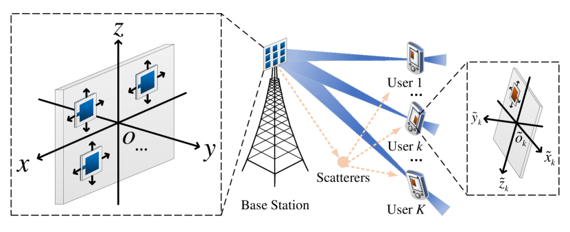
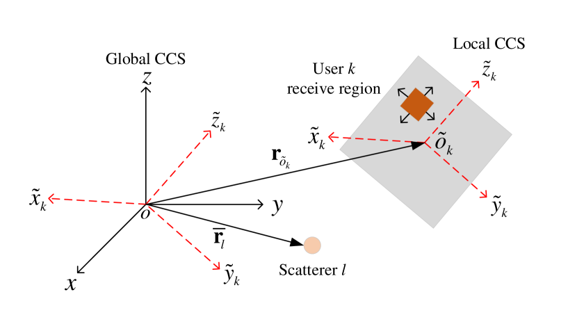
As illustrated in Fig. 1, we examine a DL transmission scenario between the BS and users. The BS is equipped with transmit MAs and user () is equipped with a single receive MA. Without loss of generality, we assume that the designated transmit and receive regions, i.e., and , for MA movements are cuboids with side lengths of and , respectively. As shown in Fig. 2, we establish a global Cartesian coordinate system (CCS) - at the BS, with the reference position of defined as the origin . The global coordinates of transmit MAs are described by , where . We also establish a local CCS - at user , with the center of defined as the origin . The local coordinates of receive MAs can be described by , where . Given that the receive regions cannot remain permanently parallel to the transmit region, we define the coordinate transform matrix between the global CCS and the local CCS at user as , where is a predetermined orthogonal matrix that satisfies [14, Sec. 8.2]. Then, denoting the coordinate of in the global CCS as , the MA position of user in the global CCS can be expressed as
| (1) |
In near-field communications, scatterers in the environment can cause multipath propagation, where the users receive signals from both LoS and NLoS paths. Thus, we consider a quasi-static near-field channel model adopting the point scatterer assumption [11]. Let denote the total number of scatterers for user and denote the coordinate of scatterer () in the global CCS. The channel vector between the transmit MAs at the BS and the receive MA at user , denoted by , can then be expressed as
| (2) |
where is the LoS component of user with the channel gain of and is the NLoS component generated by scatterer . Here, represents the complex reflection coefficient of scatterer , is the channel component between the BS and scatterer with the channel gain of , and is the channel coefficient between scatterer and user with the channel gain of , where is the carrier wavelength. Additionally, the near-field steering vector between the transmit MAs and position , i.e., , where , can be calculated as
| (3) |
For a given time slot, the BS transmits independent information streams to the users, which can be expressed as , where denotes the transmit signal with normalized power and is the corresponding beamformer. Therefore, the achievable rate of user is given by in bits per second per Hertz (bps/Hz), where is the receive signal-to-interference-plus-noise ratio (SINR) and defined as
| (4) |
where is the average noise power of user .
In this letter, we aim to minimize the transmit power at the BS by jointly optimizing the beamformers and the positions of the transmit and receive MAs. Mathematically, the optimization problem is formulated as
| (5) | ||||
Here, constraint C1 guarantees the minimum-achievable-rate requirement, , for each user. Constraint C2 restrains the restricted moving regions. Constraint C3 ensures the minimum inter-MA distance, , at the BS for practical implementation. Note that problem (5) is a highly non-convex optimization problem due to the non-convex nature of constraints C1 and C3. Furthermore, the coupling between the optimization variables renders the problem particularly intractable. Thus, we develop suboptimal solutions in the next section.
III Proposed Solution
Due to the strong coupling between the MA positions and the beamformers, conventional alternating optimization is inadequate for effectively addressing problem (5). This inadequacy arises because the MA positions (or beamformers) obtained in the previous iteration restrict the optimization space for the beamformers (or MA positions) in the current iteration [7]. To overcome this limitation, we propose a two-loop DNPPSO to simultaneously obtain high-quality suboptimal solutions while reducing computational complexity. In the inner loop, given the MA positions determined by each particle, the beamformers are optimized using semidefinite relaxation (SDR). The power consumption associated with the resulting beamformers is then incorporated into the fitness function of the outer loop to optimize the MA positions. The details are presented below.
III-A Two-Loop DNPPSO
First, we randomly initialize the positions and velocities of particles as and , respectively, where the position of each particle represents a feasible solution for the transmit and receive MA positions, i.e., (). Note that each element in satisfies constraint C2. Then, we initialize the personal best position of particle , , as , and select the global best position, , based on the fitness function, assuming that the best position has the minimum fitness value. After completing the initialization, the processing procedures of the two-loop DNPPSO algorithm are summarized in Algorithm 1. Let denote the maximum number of iterations. The details of Algorithm 1 are given as follows.
III-A1 Define Fitness Function
Given the objective to minimize the transmit power, we define the fitness function as
| (6) |
where is the position of particle in the -th () iteration. In this formulation, denotes the minimum transmit power derived from solving the following problem for any given MA positions, :
| (7) | ||||
Defining , , and , we further reformulate problem (7) as
| (8) | ||||
The semidefinite relaxation (SDR) is then applied to relax the non-convex rank-one constraints in constraint C5 by removing them, which allows the relaxed problem to be solved optimally using standard convex optimization tools. Moreover, the tightness of the rank relaxation is validated in [15, Prop. 1].
On the other hand, is the penalty function designed to ensure consistent satisfaction of constraint C3. Here, is a large positive penalty factor and is a counting function that returns the number of transmit MAs violating the minimum inter-MA distance at position . In other words, since we assume that the minimum fitness value corresponds to the best position, the penalty function can push the particles to satisfy constraint C3.
III-A2 Update Positions and Velocities
Based on the standard particle swarm optimization (PSO), the velocity and position of each particle in the -th iteration are updated as
| (9) |
| (10) |
where is a linear inertia weight function that decreases with the number of iterations within the interval to balance the exploration and exploitation, i.e., . The coefficients and are the personal and global learning factors, guiding each particle toward its personal best position and the global best position, respectively. Two random vectors and are used to avoid converging to undesired local optimal solutions, with their entries uniformly distributed within the range . The function projects each element of the vector back into the feasible region if it exceeds the allowable bound, to guarantee constraint C2.
III-A3 Dynamic Neighborhood Pruning
Once the positions of the particles are determined, the personal and global best positions are updated if the fitness value at the current position is lower than the respective personal and global minimum fitness values. Then, the algorithm initiates the pruning process.
On one hand, calculating the minimum transmit power for each particle’s position during each iteration incurs high computational overhead. On the other hand, the particles that are close to the global best position have largely exhausted the potential for discovering better positions. As such, we define the neighborhood set of the global best position as
| (11) |
where is a dynamic neighborhood radius. In each iteration, the particles within are pruned to reduce the computational overhead.
III-B Convergence and Complexity Analysis
Since only the position with a lower fitness value is selected as the global best position, the global best fitness value is non-increasing during the iterations. Besides, the transmit power is lower-bounded by zero. Therefore, the convergence of the proposed algorithm is guaranteed.
The computational complexity of Algorithm 1 primarily stems from the iterations of the two-loop DNPPSO algorithm and the process of solving problem (8) for each particle, for which the complexities are , where denotes the number of residual particles in the -th iteration, and [15], respectively. Hence, the overall complexity is .
IV Simulation Results
This section presents simulation results to validate the performance of the proposed scheme. In the simulation, the LoS and NLoS near-field channels and follow the uniform spherical wave (USW) channel model presented in [11], where the complex reflection coefficient is modeled as the circularly symmetric complex Gaussian distribution . Without loss of generality, we adopt the linear pruning strategy throughout the iterations, where the number of particles linearly decreases from the initial to with . Therefore, the computational complexity is reduced by compared to the standard PSO algorithm. Here, the linear pruning ratio, , is set to 0.02. The transmit and receive regions are set as square areas with sizes and , respectively. The carrier frequency is set to 28 GHz ( cm). The users and scatterers are uniformly distributed around the BS at distances ranging from 50 to 200 meters, within the near-field region. Unless otherwise stated, we set the moving region sizes and , the numbers of transmit antennas, users, and scatterers , , and , the average noise power dBm, the Ricean K-factor dB, the maximum numbers of iterations and particles and , the personal and global learning factors and , the minimum and maximum inertia weights and , the penalty factor , and the minimum inter-MA distance .
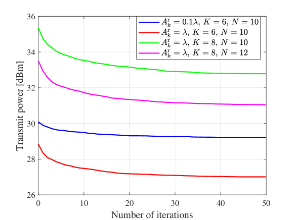
First, Fig. 3 illustrates the convergence behavior of the proposed algorithm with bps/Hz. The results show a decrease in transmit power with increasing iterations, which stabilizes within 50 iterations across all configurations. This validates the convergence analysis in Section III-B.
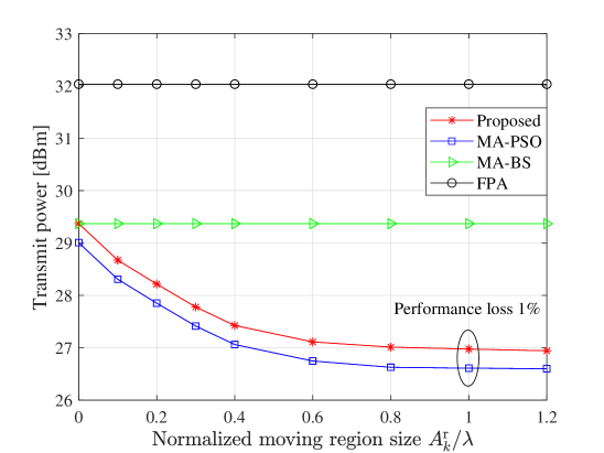
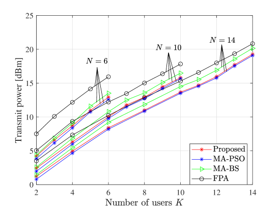
Subsequently, to fully demonstrate the advantages of the proposed scheme, we define the following benchmark schemes: (1) MA-PSO: The MA positions are optimized using the standard PSO algorithm, which is equivalent to setting . (2) MA-BS: The MAs are only equipped on the BS, and thus we have while in the proposed algorithm. (3) FPA: The BS is equipped with an FPA-based horizontal ULA with antennas spaced by , and the users are equipped with a single FPA.
Fig. 4LABEL:sub@A_UE depicts the transmit power versus the normalized moving region size at the users with bps/Hz. As can be observed, the transmit powers of the proposed and MA-PSO schemes decrease with the normalized size of the moving region and reach stable values when . This is because expanding the moving region sizes of users’ MAs enables them to utilize spatial DoFs more effectively for signal reception. Besides, the negligible performance gap between these two schemes implies that the proposed pruning strategy successfully reduces redundancy in the standard PSO algorithm. Moreover, the MA-BS and FPA schemes maintain high transmit power levels, as neither scheme implements MAs at both the BS and the users.
Fig. 4LABEL:sub@K presents the transmit power versus the number of users with bps/Hz. As the number of users increases, the transmit powers of different schemes increase due to the need to manage the multiuser interference and meet the minimum-achievable-rate requirement for each user. Compared to the FPA scheme, the MA-BS scheme partially leverages spatial DoFs to reduce power expenditure, and the proposed scheme further enhances spatial DoFs by evolving the users’ antennas into MAs, thereby reducing the power consumption even more effectively. As the number of users grows, the gap between the two schemes progressively widens. This indicates that a greater number of MAs can better exploit the DoFs across various terminals, leading to the improved performance of the communication system.
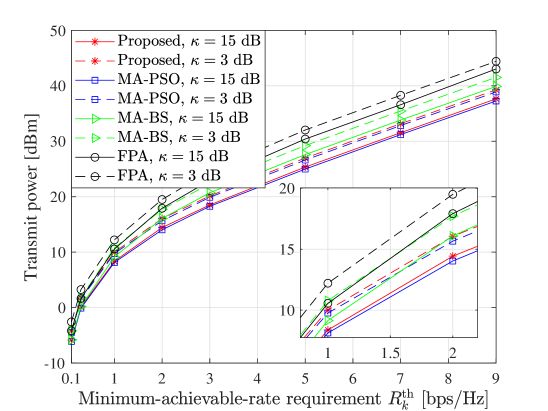
Fig. 4LABEL:sub@R shows the transmit power versus the minimum-achievable-rate requirement for each user. Intuitively, the BS has to transmit signals with higher power to meet the increased minimum-achievable-rate requirements for all users. Additionally, the schemes exhibit lower transmit power at dB compared to dB. This is because the longer transmit distance of NLoS paths compared to LoS paths leads to higher path loss. Furthermore, compared to the standard PSO algorithm, the proposed algorithm demonstrates a performance loss of only 1.04% and 1.00% at dB and dB, respectively. However, it achieves a 49% reduction in computational complexity due to , highlighting that the proposed algorithm can significantly reduce computational demands while stably maintaining performance.
V conclusion
This letter investigated an MA-aided DL multiuser system under the near-field channel condition, where both the BS and the users are equipped with MAs. To minimize the transmit power, the beamformers and the MA positions were jointly optimized using the proposed two-loop DNPPSO algorithm, which effectively maintains the performance of the standard PSO algorithm while reducing its computational complexity. Simulation results showed that the proposed scheme achieves lower power consumption compared to benchmark schemes with conventional FPAs.
References
- [1] E. G. Larsson, O. Edfors, F. Tufvesson, and T. L. Marzetta, “Massive MIMO for next generation wireless systems,” IEEE Commun. Mag., vol. 52, no. 2, pp. 186-195, Feb. 2014.
- [2] L. Zhu, W. Ma, and R. Zhang, “Modeling and performance analysis for movable antenna enabled wireless communications,” IEEE Trans. Wireless Commun., vol. 23, no. 6, pp. 6234-6250, Jun. 2024.
- [3] L. Zhu, W. Ma, and R. Zhang, “Movable antennas for wireless communication: opportunities and challenges,” IEEE Commun. Mag., vol. 62, no. 6, pp. 114-120, Jun. 2024.
- [4] L. Zhu and K.-K. Wong, “Historical review of fluid antenna and movable antenna,” arXiv preprint arXiv:2401.02362, 2024.
- [5] L. Zhu, W. Ma, and R. Zhang, “Movable-antenna array enhanced beamforming: achieving full array gain with null steering,” IEEE Commun. Lett., vol. 27, no. 12, pp. 3340-3344, Dec. 2023.
- [6] J. Ding, Z. Zhou, W. Li, C. Wang, L. Lin, and B. Jiao, “Movable antenna enabled co-frequency co-time full-duplex wireless communication,” arXiv preprint arXiv:2401.17049, 2024.
- [7] J. Ding, Z. Zhou, and B. Jiao, “New paradigm for secure full-duplex transmission: movable antenna-aided multi-user systems,” arXiv preprint arXiv:2407.10393, 2024.
- [8] W. Ma, L. Zhu, and R. Zhang, “Compressed sensing based channel estimation for movable antenna communications,” IEEE Commun. Lett., vol. 27, no. 10, pp. 2747-2751, Oct. 2023.
- [9] Z. Xiao, S. Cao, L. Zhu, Y. Liu, B. Ning, X. Xia, and R. Zhang, “Channel estimation for movable antenna communication systems: a framework based on compressed sensing,” IEEE Trans. Wireless Commun., Apr. 11, 2024, early access, DOI: 10.1109/TWC.2024.3385110.
- [10] K. Chen, C. Qi, G. Y. Li, and O. A. Dobre, “Near-field multiuser communications based on sparse arrays,” IEEE J. Sel. Top. Signal Process., Jun. 19, 2024, early access, DOI: 10.1109/JSTSP.2024.3416681.
- [11] Y. Liu, Z. Wang, J. Xu, C. Ouyang, X. Mu, and R. Schober, “Near-field communications: a tutorial review,” IEEE Open J. Commun. Soc., vol. 4, pp. 1999-2049, Aug. 2023.
- [12] Y. Chen, M. Chen, H. Xu, Z. Yang, K.-K. Wong, and Z. Zhang, “Joint beamforming and antenna design for near-field fluid antenna system,” arXiv preprint arXiv:2407.05791, 2024.
- [13] Y. Zhu, Q. Wu, Y. Liu, Q. Shi, and W. Chen, “Suppressing beam squint effect for near-field wideband communication through movable antennas,” arXiv preprint arXiv:2407.19511, 2024.
- [14] J. Diebel, “Representing attitude: euler angles, unit quaternions, and rotation vectors, Matrix, vol.58, no.15-16, pp. 1-35, Oct. 2006.
- [15] P. Guan, Y. Wang, H. Yu, and Y. Zhao, “Joint beamforming optimization for RIS-aided full-duplex communication,” IEEE Wireless Commun. Lett., vol. 11, no. 8, pp. 1629-1633, Aug. 2022.