Semi-on-Demand Off-Peak Transit Services with Shared Autonomous Vehicles —
Service Planning, Simulation, and Analysis in Munich, Germany

Abstract

This study investigates the implementation of semi-on-demand (SoD) hybrid-route services using Shared Autonomous Vehicles (SAVs) on existing transit lines. SoD services combine the cost efficiency of fixed-route buses with the flexibility of on-demand services. SAVs first serve all scheduled fixed-route stops, then drop off and pick up passengers in the pre-determined flexible-route portion, and return to the fixed route. This study addresses four key questions: optimal fleet and vehicle sizes for peak-hour fixed-route services with SAVs and during transition (from drivers to autonomous vehicles), optimal off-peak SoD service planning, and suitable use cases. The methodology combines analytical modeling for service planning with agent-based simulation for operational analysis. We examine ten bus routes in Munich, Germany, considering full SAV and transition scenarios with varying proportions of drivers. Our findings demonstrate that the lower operating costs of SAVs improve service quality through increased frequency and smaller vehicles, even in transition scenarios. The reduced headway lowers waiting time and also favors more flexible-route operation in SoD services. The optimal SoD settings range from fully flexible to hybrid routes, where higher occupancy from the terminus favors shorter flexible routes. During the transition phase, limited fleet size and higher headways constrain the benefits of flexible-route operations. The simulation results corroborate the SoD benefits of door-to-door convenience, attracting more passengers without excessive detours and operator costs at moderate flexible-route lengths, and validate the analytical model.

Keywords semi-on-demand, transit feeder, shared autonomous mobility service, transit design, flexible route

1 Introduction

1.1 Motivation

The advent of shared autonomous vehicles (SAVs) brings new perspectives to enhancing multimodal public transit services, particularly as feeders in less dense areas (Ng et al. 2024b). With lower operating costs, they can address the first-mile-last-mile problem and bring passengers to other transit modes more efficiently than conventional ride-sharing. While transit agencies retain some drivers due to union contracts or operational reasons, the lower operating costs of SAVs also allow for a larger fleet of smaller vehicles and thereby more frequent services (Hatzenbühler et al. 2020). Transit agencies can plan their fleet (vehicle size and type) according to peak-hour fixed-route service, which leaves redundant capacity at off-peak times for more flexible services and expand their catchment areas. For example, smaller but more SAVs can pick up and drop off some passengers at their homes, bringing more convenience and stimulating more demand (Frei et al. 2017).

In semi-on-demand (SoD) hybrid-route services investigated in previous studies (Ng and Mahmassani 2023, Ng et al. 2024a) (Figure 1), SAVs first serve all fixed-route stops based on a schedule, then drop off and pick up passengers in the flexible-route portion (pre-determined with length $x_{f}$), and return to fixed-route scheduled stops and the terminus. It is shown to combine the cost efficiency of fixed-route buses in denser areas with the flexibility of on-demand services in less populated regions.

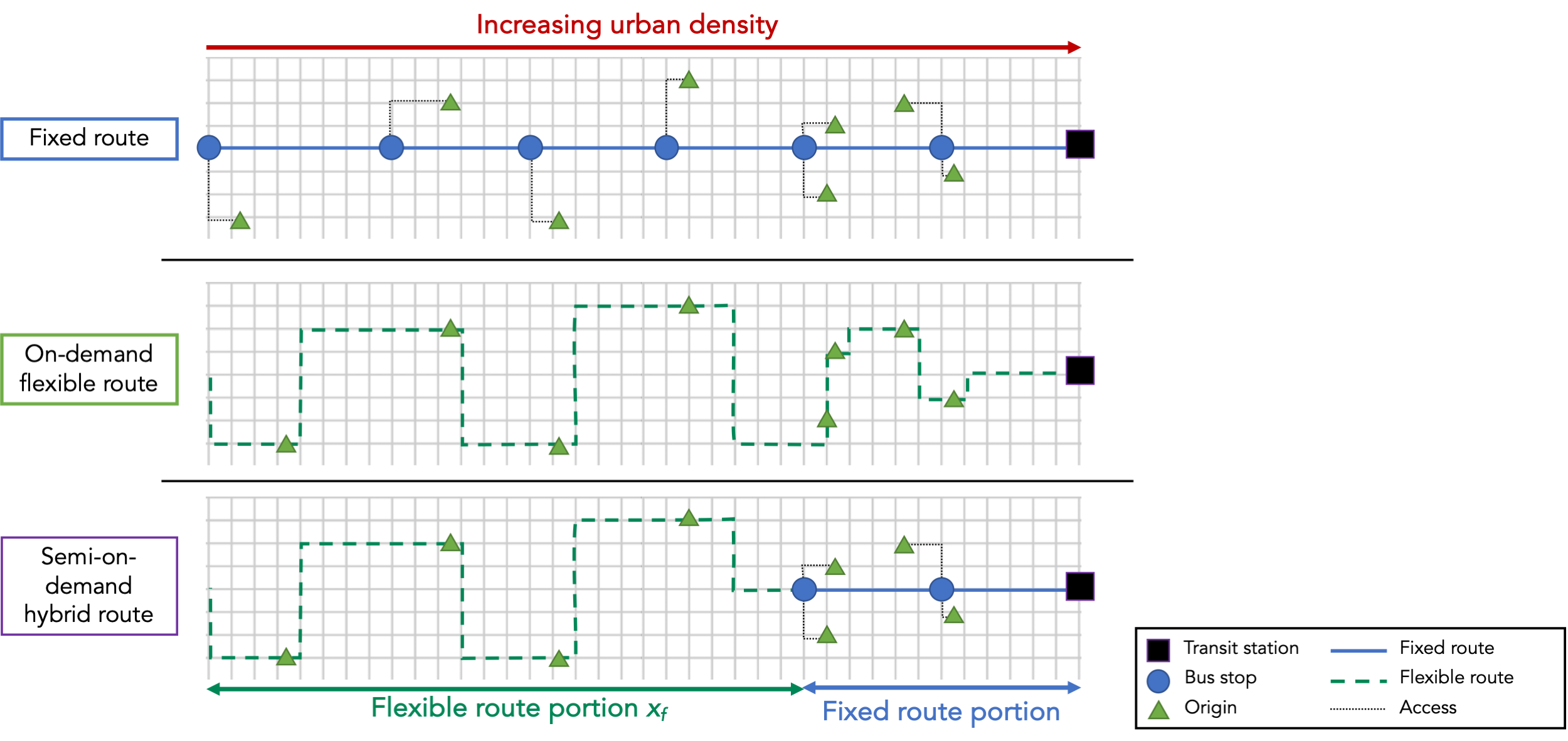
Figure 1: Illustration of semi-on-demand hybrid route as a feeder service

1.2 Problem Description

This study considers improving current transit services with SAVs by enhancing peak-hour fixed-route service (in the existing format but more frequent due to SAV cost savings) and implementing off-peak SoD hybrid-route services in the same route catchment area. We address four primary research questions:

1. At peak hours, what are the optimal fleet and vehicle sizes for current-day transit lines with the lower operating costs of SAVs, when we minimize waiting time and operator’s cost subject to capacity and budget constraints?

2. During a transition phase from drivers to full automation, how would the operating budget affect the previous optimal results?

3. At off-peak hours, what is the optimal service planning (schedule and route form) for SoD hybrid-route services, considering stochastic requests and balance between schedule time, request rejection, and operational performance?

4. What are the use cases of off-peak SoD services considering benefits and impacts to passengers and the operator?

For SoD, too long flexible routes would lead to excessive detours, longer journey times, and higher operating costs. Meanwhile, smaller headways (e.g., more smaller vehicles) favor longer flexible routes by reducing the detours of each trip (Ng et al. 2024a). Therefore, optimizing SAV fleet and vehicle sizes for peak-hour fixed routes may also benefit off-peak SoD hybrid-route services.

The problem scope is defined with some key assumptions: (i) continuous operations during the study hours; (ii) inelastic demand (yet sensitive to walking distance); (iii) requests made when passengers are ready for boarding, with no reservations considered; and (iv) individual travelers, i.e. no group bookings are considered.

1.3 Contributions

Building upon the theoretical formulations of costs and benefits derived in previous work (Ng et al. 2024a), this study focuses on the service planning, simulation, and analysis of the SoD hybrid-route transit feeders using SAVs. It presents conceptual, theoretical, and methodological contributions:

1. We formulate the service planning problem of peak-hour fixed-route services in terms of optimal fleet size and vehicle size, considering changes in costs and retention of drivers. The study further conceptualizes the off-peak SoD hybrid-route service.

2. We derive analytical results of convex optimization for the peak-hour fleet and vehicle sizes (in full-SAV and partial-driver scenarios) and off-peak schedules considering detours, service guarantee, and peak/off-peak service level. This is a timely addition to the literature for planning the gradual introduction of SAVs in transit service.

3. By analyzing the agent-based simulation results on ten existing bus routes in the city of Munich, Germany, we optimize the flexible-route portion $x_{f}$ and headway $h$, and examine the use cases and benefits of hybrid routes (in terms of access, waiting, and riding times for users and vehicle distances and requirements for operators). We contrast theoretical predictions with simulation results and study variations in user experience.

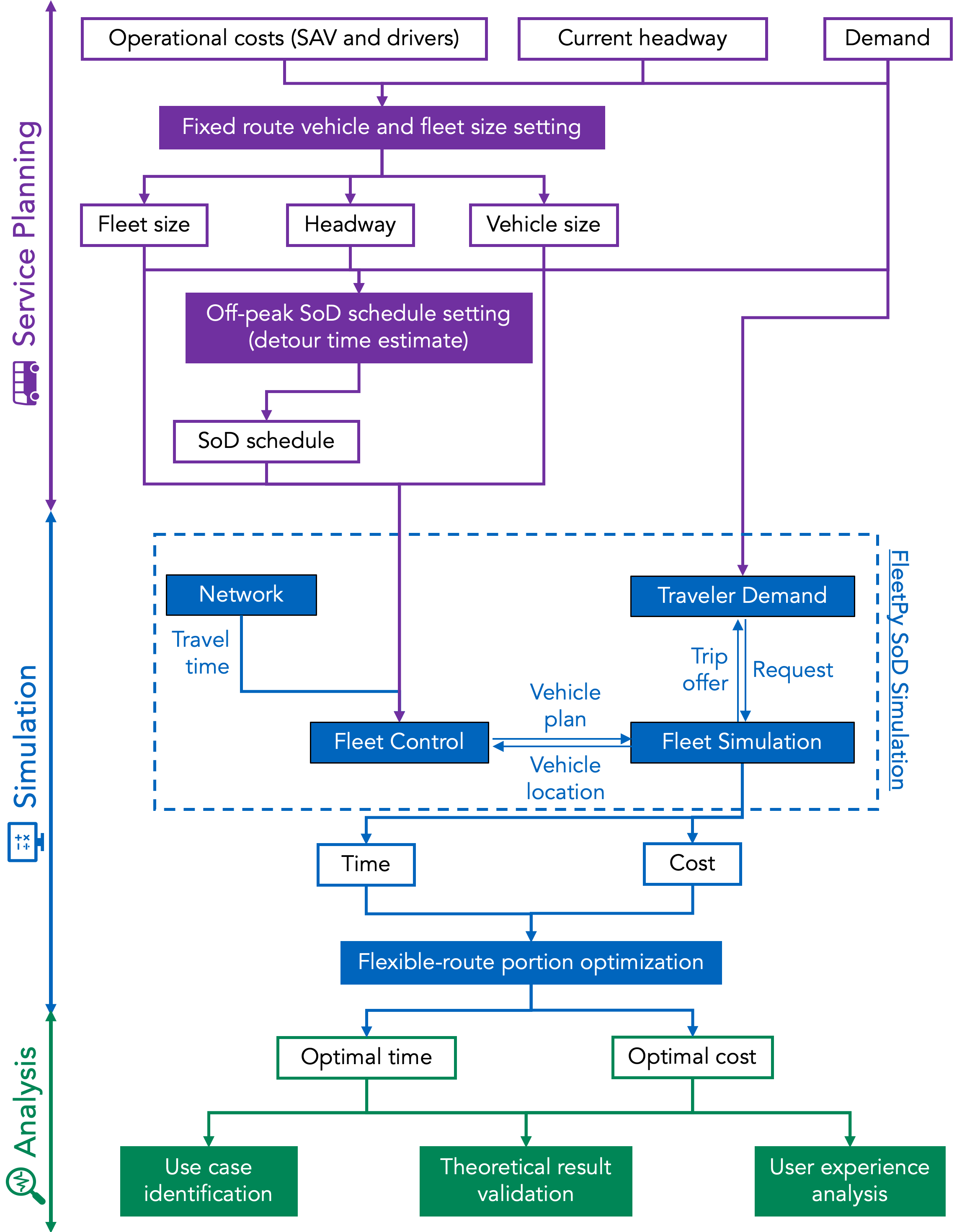
Figure 2: Flowchart of the service planning, simulation, and analysis

Figure 2 summarizes the flow of the methodology. The remainder of the paper is structured as follows. Section 2 presents an overview of relevant literature on demand-responsive transit, SAVs in public transit, and ride-sharing simulation. Section 3 follows with the methodology, illustrated with an experiment described in Section 4 and results presented in Section 5. Section 6 concludes the paper.

2 Background

2.1 Demand-Responsive Transit

Research on demand-responsive transit (DRT) spans a few decades (see surveys by Errico et al. (2013), Vansteenwegen et al. (2022)). Several studies have explored flexible transit route designs, suggesting conditions to use demand-responsive over fixed-route services (Li and Quadrifoglio 2010) and cost advantages for low-to-moderate passenger demand (Nourbakhsh and Ouyang 2012). Recent research has focused on integrating DRT with traditional fixed services, e.g., supplementary DRT improvements to fixed-route bus services (Chen and Nie 2017) and combination of fixed-schedule and DRT services during off-peak hours and in the suburbs (Calabrò et al. 2023).

Various optimization strategies have been employed in semi-flexible transit system research, including analytical models (Qiu et al. 2014), metaheuristics (Galarza Montenegro et al. 2021), stochastic approaches with Markov decision processes (Rambha et al. 2016, Li et al. 2023), and agent-based simulation (Rich et al. 2023).

However, most studies focus on the performance of flexible-route services or the decision to deploy either flexible-route or fixed-route services. In contrast, this study builds on previous work (Ng et al. 2024a) to design and simulate hybrid-route service, representing a continuum between these two service modes.

2.2 Shared Autonomous Vehicles in Public Transit Systems

SAVs have shown the potential in expanding transit coverage and enhancing service attractiveness (Salazar et al. 2020, Shen et al. 2018) (also see the survey by Narayanan et al. (2020)). Several studies have explored the synergistic relationship between SAVs and public transit systems (Shen et al. 2018, Cortina et al. 2023, Gurumurthy et al. 2020a), sometimes by integrating SAVs into traditional transit (Levin et al. 2019). Conversely, some considered SAVs as competitors (Sieber et al. 2020), with performance improvements by replacing fixed bus routes with flexible routes in suburbs in Chicago, USA (Ng and Mahmassani 2023, Volakakis et al. 2023). The joint design of transit and SAVs has been another area of focus, e.g., optimizing vehicle size (Alonso-Mora et al. 2017), fleet size (Pinto et al. 2020, Dandl et al. 2021), network (Ng et al. 2024b), and timetabling and vehicle scheduling (Cao and Ceder 2019).

Automation can also benefit line-based buses, with a general shift towards higher frequencies and smaller vehicles (Bösch et al. 2018) found to attract passengers through improved service (Hatzenbühler et al. 2020) and SAVs as feeders to improve efficiency (Badia and Jenelius 2021).

In summary, the integration of SAVs in public transit systems presents opportunities for improved service quality, expanded coverage, and enhanced operational efficiency. However, challenges remain in optimizing the balance between traditional fixed-route services and more flexible autonomous options across urban contexts and demand patterns.

2.3 Ride-Sharing Simulation

Agent-based simulation has been widely used to represent the dynamic and stochastic nature of underlying vehicle routing problems and the interaction between operators and riders. Studies focused on solving the online assignment problem (Alonso-Mora et al. 2017, Simonetto et al. 2019, Wang et al. 2023) or repositioning idle vehicles to accommodate future expected demand (Zhang and Pavone 2016, Tafreshian et al. 2021, Engelhardt et al. 2024). Apart from door-to-door services, short walking legs for riders (Engelhardt and Bogenberger 2021, Fielbaum et al. 2021) or transfers between vehicles (Masoud and Jayakrishnan 2017, Namdarpour et al. 2024) have been proposed to increase efficiency and sharing rate for the service.

On the operational aspects of demand-responsive services, models like SUMO (Armellini 2021), MATSim (Horni et al. 2016), and Polaris (Gurumurthy et al. 2020b, Cokyasar et al. 2022) have been extended to simulate both fixed- and flexible-route services. Other studies have developed new agent-based simulation models focusing on operational aspects or computational performance (Alonso-Mora et al. 2017, Fagnant and Kockelman 2018, Dandl et al. 2019, Engelhardt et al. 2022). These studies focused on the supply side, i.e., how to serve a fixed set of riders as efficiently as possible. Meanwhile, agent-based demand models (Ruch et al. 2018, Gurumurthy et al. 2020c, Wilkes et al. 2021) have been developed to estimate the demand attracted to the new modes.

This study adapts the open-source Python package Fleetpy (Engelhardt et al. 2022) to model the hybrid-route SoD service and the interaction between riders, operator, and vehicles.

3 Methodology

This section first discusses the service planning for peak-hour fixed-route service in full SAV and transition scenarios, followed by off-peak SoD schedule setting. It then describes the simulation of SoD service and result analysis.

The notations used are summarized in Table LABEL:tab:notation.

Table 1: Notation

Symbol	Description	Experiment Value
$a_{i,z}$	Arrival time of passenger $i$ according to plan $z$
$b\in\mathcal{B}$	Vehicle size	$\mathcal{B}=\{5,8,20,44,70\}~{}pax$
$c^{g}$	Total generalized cost
$c^{o}_{v}$	Vehicle cost of vehicle $v$
$c^{u}_{r}$	User cost of rider $r$
$C_{v}$	Vehicle capacity of vehicle $v$
$c(b,h)$	Cost function of a route with vehicle size $b$ and headway $h$
$d_{r}$	Destination node of request $r$
$d_{r}^{f}$	Nearest bus stop to the destination of request $r$
$d_{v,z}$	Distance traveled by vehicle $v$ according to plan $z$
$D$	Total detour distance (R.V.)
$D^{p}$	Peak demand
$D^{w}$	Maximum walking distance	500 m
$E_{i}$	Earliest start time for stop $i$
$\mathcal{E}$	Edges of the network
$\mathcal{G}$	Street network
$h$	Headway
$h^{*}$	Optimal headway
$h^{p}$	Peak-hour headway
$H^{0}$	Existing headway
$i\in\mathcal{I}$	Stop
$L^{x}$	Route length
$N^{a}$	Number of SAVs
$N^{d,0}$	Current number of drivers
$n^{r}_{z}$	Number of requests satisfied in vehicle plan $z$
$n^{s}_{z}$	Number of requests served in the fixed route in vehicle plan $z$
$N$	Number of flexible-route requests (R.V.)
$\mathcal{N}$	Nodes of the network
$o_{r}$	Origin node of request $r$
$o_{r}^{f}$	Nearest bus stop to the origin of request $r$
$r\in\mathcal{R}$	Customer request
$s$	Fleet size
$t^{a}_{r}$	Access time of request $r$
$t^{d}_{c}$	Allowable vehicle detour time
$t^{t}_{r}$	Riding time of request $r$
$t^{v}_{v}$	Time deployed for vehicle $v$
$t^{w}_{r}$	Waiting time of request $r$
$t_{r}$	Request time of request $r$
$T$	Total expected detour time (R.V.)
$T^{c}$	Cycle time
$T^{l}_{i}$	Latest start time for stop $i$
$T^{s}$	Dwell time	30 s
$T^{s}_{i}$	Duration of stop $i$
$T^{w,max}$	Maximum waiting time	15 min
$v\in\mathcal{V}$	Vehicle
$V^{d}$	Constant vehicle speed (in planning)	40 km/h
$X$	Irwin-Hall distribution R.V.
$Y$	Detours for requests (R.V.)
$Y_{i}$	Stop location of stop $i$
$z$	SoD schedule
$\alpha$	Portion of original drivers remaining in the workforce
$\gamma^{a}$	Cost coefficient for access time	2
$\gamma^{c}_{b}$	Operational costs (operating + capital) of SAV size $b$	{4.4, 5.9, 11.05,
		16.2, 23.8, 33.9} (€/h)
$\gamma^{c,0}$	Current bus HDV operational cost	€36.3/h
$\gamma^{d}$	Driver cost	€15.3/h
$\gamma^{f}$	Reward coefficient for fixed-route requests	1e+6
$\gamma^{m}_{b}$	Operating costs of SAV size $b$ per hour	{2.1, 2.6, 4.15,
		5.7, 9.5, 12.6} (€/h)
$\gamma^{m,0}$	Current bus HDV operating cost	€24.8/h
$\gamma^{o}_{v}$	Cost coefficient for vehicle distance of vehicle $v$
$\gamma^{r}$	Cost coefficient for traveler time	€16.5/h
$\gamma^{s}$	Reward coefficient for requests satisfied	1e+6
$\gamma^{t}$	Value of time	€16.5/h
$\gamma^{v}_{v}$	Cost coefficient for vehicle time of vehicle $v$
$\gamma^{w}$	Cost coefficient for waiting time	1.5
$\lambda$	Poisson distribution parameter
$\Lambda$	Demand
$\phi^{p}$	Maximum in-vehicle travel time factor	2
$\rho$	Capacity buffer	0.9
$\phi(z)$	Objective function for schedule $z$

3.1 Service Planning

3.1.1 Optimal Vehicle and Fleet Size for Peak-Hour Fixed-Route Service - Full SAV Scenario

For a peak-hour fixed route with 100% SAVs, we develop a convex optimization problem with analytical closed-form solutions of vehicle size $b$ and headway $h$, subject to capacity and budget constraints. The goal is to minimize $c(b,h)$ in Eq. 1, the weighted sum of users’ waiting time and operator’s cost (including both capital and operating expenses). The first term is the waiting cost with the value of time $\gamma^{t}$, waiting cost coefficient $\gamma^{w}$, and demand $\Lambda$. The second term is the operational (capital and operating) cost to run a fleet with $s=T^{c}/h$ vehicles with the unit cost per time $\gamma^{c}_{b}$ and cycle time $T^{c}$.

$$c(b,h) =\frac{1}{2}\gamma^{t}\gamma^{w}\Lambda h+\gamma^{c}_{b}\frac{T^{c}}{h}$$ (1)

For the optimality condition with respect to $h$, we set the first partial derivative in Eq. 2 to zero. The cost function is also shown to be convex as the second derivative in Eq. 3 is always positive.

$$\frac{\partial c}{\partial h} =\frac{1}{2}\gamma^{t}\gamma^{w}\Lambda-\gamma^{c}_{b}\frac{T^{c}}{h^{2}}$$ (2)

$$\frac{\partial^{2}c}{\partial h^{2}} =2\gamma^{c}_{b}\frac{T^{c}}{h^{3}}>0$$ (3)

This leads to the optimal headway $h^{*}$ in Eq. 4, resulting in the minimum cost $c^{*}(b)$ in Eq. 5. $h^{*}$ is inversely proportional to the square root of demand density, which bears similarity to the result of Newell (1979).

$$h^{*} =\sqrt{\frac{2\gamma^{c}_{b}T^{c}}{\gamma^{t}\gamma^{w}\Lambda}}$$ (4)

$$c^{*}(b) =\sqrt{2\gamma^{t}\gamma^{w}\gamma^{c}_{b}\Lambda T^{c}}$$ (5)

To ensure sufficient line capacity, $h$ is bounded above in Eq. 6 (given vehicle size $b$ and capacity buffer $\rho\in[0,1]$) to satisfy peak demand $D^{p}$. This corresponds to the minimum cost in Eq. 7 for each vehicle size. To find the lowest-cost solution that provides sufficient capacity, we iterate through all discrete $b$.

$$h \leq\frac{b\rho}{D^{p}}$$ (6)

$$c^{b}(b) \geq\frac{1}{2}\gamma^{t}\gamma^{w}b\rho+\gamma^{c}_{b}\frac{D^{p}T^{c}}{b}\rho$$ (7)

To comply with the existing operating budget, $h$ is bounded below in Eq. 8 (with existing operating unit cost $\gamma^{c,0}$ and headway $H^{0}$). Combining this with Eq. 6 brings us Eq. 9, which checks whether a vehicle size can fulfill both capacity and budget constraints.

$$h \geq\frac{\gamma_{b}^{c}}{\gamma^{c,0}}H^{0}$$ (8)

$$b \geq\frac{\gamma_{b}^{c}}{\gamma^{c,0}}\frac{H^{0}D^{p}}{\rho}$$ (9)

In short, we find $h^{*}$ in Eq. 4 subject to the upper bound in Eq. 6 and lower bound in Eq. 8. If Eq. 9 is violated, the upper bound for $h$ is lower than the lower bound, and there is no feasible solution for that particular vehicle size $b$.

3.1.2 Optimal Vehicle and Fleet Size for Peak-Hour Fixed-Route Service - Transition Scenario with Drivers

The transition scenario is motivated by a socially responsible path towards SAV-based public transit that retains drivers in the workforce until their redeployment/retirement. For simplicity, they are assumed to drive some SAVs in the new fleet (same vehicle size for each route). We adapt the previous optimization procedure by detaching capital costs from overall operational cost, under the assumption that the capital investment decision is already made for a long-term full rollout scenario. Hence, the equations in the previous subsection are still valid, except that $\gamma^{c}_{b}$ is replaced by $\gamma^{m}_{b}$. The question is whether we can still improve some services by replacing a bus with smaller SAVs while maintaining budget balance and satisfying capacity.

The operating budget in the transition period is composed of labor costs ($\gamma^{d}$ per remaining driver) and SAV operating costs (unit cost $\gamma^{m}_{b}$). When a portion $\alpha$ of the original $N^{d,0}$ drivers remain in the workforce, and an additional SAV fleet of $N^{a}$ is added to provide services, i.e., the fleet size becomes $s=\alpha N^{d,0}+N^{a}$. The total operating costs are subject to the current budget (unit operating cost $\gamma^{m,0}$ and labor cost) in Eq. 10.

$$\gamma^{m}_{b}(\alpha N^{d,0}+N^{a})+\gamma^{d}\alpha N^{d,0}\leq(\gamma^{m,0}+\gamma^{d})N^{d,0}$$ (10)

This can be rearranged as an upper bound on the fleet size $s$ in Eq. 11 or a lower bound on the headway in Eq. 12.

$$s \leq\frac{\gamma^{m,0}-\gamma^{d}(1-\alpha)}{\gamma^{m}_{b}}N^{d,0}$$ (11)

$$h \geq\frac{\gamma^{m}_{b}}{(\gamma^{m,0}-\gamma^{d}(1-\alpha))}H^{0}$$ (12)

3.1.3 Off-Peak Semi-on-Demand Schedule Setting

An SoD schedule is formed by fixed stops (existing route schedule) and the flexible-route portion (with length $x_{f}$ in Figure 1, existing journey time plus allowable vehicle detour time $t^{d}_{c}$). Serving a certain level $c$ (say 95%) of stochastic demand in the flexible-route portion requires an adequate $t^{d}_{c}$. We derive its cumulative distribution function with the assumptions of (i) independently uniformly distributed detours for each request ($Y\sim\text{Uniform}(0,D^{w})$), (ii) Poisson occurrences of flexible-route requests ($N\sim\text{Poisson}(\lambda)$), and (iii) constant vehicle speed $V^{d}$.

The total detour distance $D$ given $N$ requests is the sum of detours (multiplied by two for deviating from and returning to the main route) in Eq. 13. The total detour time given the number of request points, $T|N$, is the sum of dwell times and total detour time in Eq. 14.

$$D|N =\sum_{r=1}^{N}2Y$$ (13)

$$T|N =NT^{s}+\frac{D|N}{V^{d}}=NT^{s}+\sum_{r=1}^{N}\frac{2Y}{V^{d}}$$ (14)

We note that $T|N$, as a sum of uniform distributions ($Y$), follows the Irwin-Hall distribution with a cumulative distribution function (CDF) in Eq. 15 (Johnson et al. 1995). By considering $\sum_{r=1}^{N}Y=V^{d}/2(T|N-NT^{s})$ from Eq. 14 and normalizing it by setting $X=\sum_{r=1}^{N}Y/D^{w}$ (so that the support of $X|N$ is $[0,N]$), we obtain the CDF of $T|N$ in Eq. 16.

$$P(X\leq x) =\frac{1}{n!}\sum_{k=0}^{\lfloor x\rfloor}(-1)^{k}\binom{n}{k}(x-k)^{n}$$ (15)

$$P(T\leq t^{d}_{c}|N=n) =P\left(X\leq\frac{V^{d}}{2D^{w}}(t^{d}_{c}-nT^{s})\right)$$ (16)

As the occurrence of flexible-route requests $N$ follows a Poisson distribution, its probability mass function is given in Eq. 17.

$$P(N=n) =\frac{e^{-\lambda}\lambda^{n}}{n!}$$ (17)

By the law of total probability, we get $P(T\leq t^{d}_{c})=\sum_{n=0}^{\infty}P(T\leq t^{d}_{c}|N=n)P(N=n)$. This leads to the CDF of $T$ in Eq. 18. The corresponding $t^{d}_{c}$ for the required confidence level of demand satisfaction can then be approximated from the CDF curve.

$$P(T\leq t^{d}_{c}) =\sum_{n=0}^{\infty}\frac{e^{-\lambda}\lambda^{n}}{(n!)^{2}}\sum_{k=0}^{\lfloor x\rfloor}(-1)^{k}\binom{n}{k}(x-k)^{n},$$

$$\text{where }x=\frac{V^{d}}{2D^{w}}(t^{d}_{c}-nT^{s})$$ (18)

Afterward, we consider the constraint posed by the vehicle requirements of a schedule. Taking fleet size $s$ that is set in the previous subsection based on the peak-hour fixed route operating with a headway $h^{p}$ and a cycle time of $T^{c}$, we have $s=T^{c}/h^{p}$. For SoD services at off-peak hours with the same fleet size $s$ but headway $h<h^{p}$, the additional detour $t^{d}_{c}$ poses a more stringent requirement on $s$, i.e., $s\geq(T^{c}+t^{d}_{c})/h$. Combining the two equations suggests an upper bound of $t^{d}_{c}$ in Eq. 19.

$$t^{d}_{c} \leq T^{c}\left(\frac{h}{h^{p}}-1\right)$$ (19)

These equations are used to design schedules for SoD services in different lines and yield statistical insights into the trade-offs between service guarantee, performance, and operating costs.

3.2 Simulation of Semi-on-Demand Service

We expand the FleetPy simulation framework (Engelhardt et al. 2022) with an SoD module (Figure 2). It models the interaction among three agents: riders $r\in\mathcal{R}$, a service operator, and vehicles $v\in\mathcal{V}$ within a street network $\mathcal{G}=(\mathcal{N},\mathcal{E})$ with nodes $\mathcal{N}$ and edges $\mathcal{E}$ in discrete time steps. Customers request trips (with demand as a function of access distance), where each rider request $r$ is defined by the request time $t_{r}$, origin $o_{r}\in\mathcal{N}$, and destination $d_{r}\in\mathcal{N}$. The operator evaluates requests, considers service quality and operational constraints (e.g., maximum waiting and travel times and vehicle capacity), and assigns requests to individual vehicles operating on SoD schedules $z$. A schedule is an ordered list of stops that are processed by the vehicle one after another, whereas a stop $i\in\mathcal{I}$ is characterized by a location $Y_{i}\in\mathcal{N}$, the latest start time $T^{l}_{i}$, the earliest start time $E_{i}$, a duration $T^{s}_{i}$, and sets of requests boarding and alighting the vehicles.

In between stops, vehicles travel in the network on the fastest path. If they arrive at the next stop $i$ before the scheduled time $E_{i}$, they wait there until $E_{i}$. In the next step, they perform the boarding task associated with this stop for a duration of $T^{s}_{i}$ and then go to the next stop.

Requests are assigned by sequential insertion into currently assigned vehicle schedules. The feasibility of each resulting schedule is then evaluated based on the following constraints: (i) each stop $i$ in the schedule is served no later than $T^{l}_{i}$; (ii) each rider waits less than the maximum waiting time $T^{w,max}$; (iii) the maximum in-vehicle travel time of each passenger is within the direct travel time by a factor $\phi^{p}$; and (iv) the number of passengers never exceeds the vehicle capacity $C_{v}$.

The objective $\phi(z)$ of all feasible schedules is then calculated in Eq. 20 that balances vehicle distance, rider travel time, and requests served in the fixed-route portion. $\gamma^{o}_{v}$, $\gamma^{t}$, $\gamma^{r}$, and $\gamma^{s}$ are the cost/reward coefficients for vehicle distance, traveler time, requests satisfied, and requests served in a fixed route, respectively. $d_{v,z}$, $a_{r,z}$, $n^{r}_{z}$, and $n^{s}_{z}$ are respectively the distance traveled by vehicle $v$, arrival time of rider $r$, number of requests satisfied, and number of requests served in a fixed route.

$$\phi(z) =\sum_{v\in\mathcal{V}}\gamma^{o}_{v}d_{v,z}+\sum_{r\in\mathcal{R}}\gamma^{t}(a_{r,z}-t_{r})-\gamma^{r}n^{r}_{z}-\gamma^{s}n^{s}_{z}$$ (20)

The feasible schedule with the minimum objective is then selected and assigned. The process is summarized as follows:

1. If a rider request $r$ is picked up or dropped off in the fixed-route portion, $o_{r}$ or $d_{r}$ is shifted to $o_{r}^{f}$ or $d_{r}^{f}$ corresponding to the nearest bus stop.

2. A request is assigned to the vehicle schedule by: (i) adding the request to the boarding or alighting list of a stop if the corresponding locations match; or (ii) inserting a new stop to pick up or drop off the request. All feasible insertions for a request and each vehicle are computed by an exhaustive search, and the schedule $z$ that minimizes $\phi(z)$ in Eq. 20 is assigned. If no feasible insertion is found, the rider’s request is rejected.

3. Steps 1 and 2 are repeated until all current requests are processed. Then, vehicles move and perform boarding processes according to their assigned schedules.

The simulation records user and vehicle data on trip level and at the end of the simulation, metrics in aggregate terms are computed.

3.3 Analysis

The simulation results of each scenario (each flexible-route length $x_{f}$) are analyzed and compared to identify the suitable use cases for SoD. Generalized costs are used as metrics that include both user’s and operator’s costs.

The user’s cost $c^{u}_{r}$ of rider $r$ in Eq. 21 is composed of access (walking), waiting, and riding costs, where $t^{a}_{r}$, $t^{w}_{r}$, and $t^{t}_{r}$ are the access, waiting, and riding times and $\gamma^{a}$, $\gamma^{w}$, and $\gamma^{r}$ are the respective cost coefficients.

$$c^{u}_{r} =\gamma^{a}t^{a}_{r}+\gamma^{w}t^{w}_{r}+\gamma^{r}t^{t}_{r}$$ (21)

The vehicle cost $c_{v}^{o}$ for vehicle $v$ in Eq. 22 consists of distance-based operating cost and vehicle marginal cost, where $d_{v}$ and $t^{v}_{v}$ are the distance traveled and time deployed with $\gamma^{o}$, and $\gamma^{v}$ as the respective cost coefficients.

$$c^{o}_{v} =\gamma^{o}_{v}d_{v}+\gamma^{v}_{v}t^{v}_{v}$$ (22)

The total generalized cost $c^{g}$ in Eq. 23 is the sum of all users’ costs and operator’s costs.

$$c^{g} =\sum_{r\in\mathcal{R}}c^{u}_{r}+\sum_{v\in\mathcal{V}}c^{o}_{v}$$ (23)

The optimal SoD route form may be fixed route ($x_{f}=0$), hybrid route ($0\leq x_{f}\leq L^{x}$), or flexible route ($x_{f}=L^{x}$), depending on the minimum generalized cost $c^{g}$ and number of passengers served. We identify such cases and also analyze the more fine-grained effects on journey time and operational costs, in comparison with the theoretical values (Ng et al. 2024a).

4 Experiment Design

We selected ten bus routes in eastern Munich, Germany (Figure 3) with different characteristics. Routes 1, 3, and 5 offer frequent service with at most 10-minute headways, serving as longer routes that connect suburbs to the city center. Routes 2 and 4 provide less frequent service with 20-minute headways with similar purposes. The remaining Routes 6-10 primarily function as feeder routes to and from U-Bahn/S-Bahn train stations.

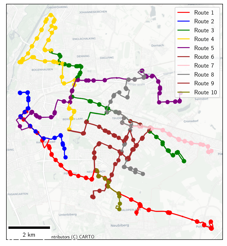
Figure 3: Ten bus routes studied in Munich, Germany

Monte Carlo simulations are conducted to model the SoD service under each scenario, as defined by route, flexible-route portion $x_{f}$ (in km increment), and driver proportion (0%, 75%, 100%), with 100 generated demand instances. The simulation runs from 9 pm to midnight to capture off-peak demand, with the first hour excluded from metric evaluation to allow for warm-up. Trip origins and destinations are derived from a boarding and alighting dataset provided by a local public transit operator. Demand modeling follows a previously established local logit model that is sensitive to walking time (Moeckel et al. 2020).

Parameter values used in the simulation are included in Table LABEL:tab:notation. Table 2 provides an overview of route characteristics. Other data sources include GIS dataset of transit alignment and stop locations (MVG 2024), road network with steady travel time (Boeing 2017), and SAV cost (Tirachini and Antoniou 2020).

Table 2: Route characteristics and optimal service planning results

Route ID	1	2	3	4	5	6	7	8	9	10
Route Information
Length $L^{x}$ (km)	9.9	5.4	10.7	11.9	11.5	6.8	5.6	4.3	5.8	3.1
Cycle Time $T^{c}$ (min)	90	40	70	80	80	40	40	70	60	20
Peak-Hour Demand $\Lambda$ (pax/h)	622	114	498	94	248	430	351	244	211	188
Off-Peak Demand (pax/h)	227	65	77	20	134	110	138	25	36	59
Peak-Hour Headway $H^{0}$ (min)	6	20	5	20	10	7.5	10	10	10	15
Vehicle size (pax)	70	70	70	70	70	70	70	70	70	70
Fleet size (veh)	15	2	14	4	8	6	4	7	6	2
Optimal Results - Full SAV Scenario
Peak-Hour Headway $h^{*}$ (min)	3	3.5	1	3	2	3	3.5	2	1.5	5.5
Vehicle size $b^{*}$ (pax)	44	8	8	5	8	20	20	8	5	20
Fleet size $s^{*}$ (veh)	32	12	80	28	46	16	13	40	47	4
Off-Peak Headway $h$ (min)	5	5	5	10	3	5	5	10	8	8
Optimal Results - 75% Drivers ($\alpha=0.75$)
Peak-Hour Headway $h^{*}$ (min)	3	7	2	3.5	3.5	3	5	2	2	5.5
Vehicle size $b^{*}$ (pax)	44	20	20	8	20	20	44	8	8	20
Fleet size $s^{*}$ (veh)	32	6	45	24	26	16	8	40	30	4
Off-Peak Headway $h$ (min)	5	10	5	10	5	5	8	10	8	8
Optimal Results - 100% Drivers ($\alpha=1$)
Peak-Hour Headway $h^{*}$ (min)	4	10	2.5	4	3.5	4	7	4	5	5.5
Vehicle size $b^{*}$ (pax)	44	20	20	8	20	44	44	20	20	20
Fleet size $s^{*}$ (veh)	25	4	34	20	25	10	6	18	13	4
Off-Peak Headway $h$ (min)	5	15	5	10	5	6	10	10	8	10

5 Results

This section begins by discussing the results of service planning for peak-hour fixed routes, considering both full SAV and transition scenarios, followed by the SoD schedule setting. We then analyze the simulation results of SoD service operations. Finally, we examine the SoD use cases, deviations from theoretical values, and variations in user experience.

5.1 Service Planning

5.1.1 Optimal Vehicle and Fleet Size for Peak-Hour Fixed-Route Service - Full SAV Scenario

Table 2 shows considerable improvements in service quality under the full SAV scenario. Peak-hour headways are substantially reduced, e.g., from 6 min to 3 min for Route 1. Besides, optimal vehicle sizes trend towards smaller. The original 70-passenger buses are replaced by 44-passenger vehicles for Route 1, or even by smaller 8-passenger or 5-passenger cars for some other routes. These changes, due to cost savings from SAVs, improve service quality with lower waiting times while keeping current operating costs. The larger fleet sizes also provide extra capacity for SoD at smaller off-peak headways, which means fewer detours in each run.

5.1.2 Optimal Vehicle and Fleet Size for Peak-Hour Fixed-Route Service - Transition Scenario with Drivers

We examined scenarios with varying percentages of drivers ($\alpha=100\%,75\%$) to understand the optimal configuration during the transition.

From Table 2, the 100% driver scenario results involve much higher headways and larger vehicles compared to the full SAV scenario. Instead of 8-passenger vans on Routes 2 and 3 (full SAV scenario), 20-passenger minibuses are used. The 75% driver scenario falls between full drivers and SAV scenarios. Notably, even during the transition with drivers in SAVs, service quality improvements and waiting time reductions are achievable by switching to a fleet of smaller SAVs on less busy routes. Nevertheless, this is based on assumptions that vehicle sizes for a route can be switched easily (e.g., from a pool of vehicles shared by various routes). Otherwise, some routes may need to wait for lower driver proportions to reap the full benefits, which means the focus could be laid on high-demand routes first.

5.1.3 Off-Peak Semi-on-Demand Schedule Setting

Figure 4 illustrates the theoretical cumulative distribution of detour time $T$ in Eq. 18 under different $x_{f}$ for Route 7 as an example. Higher service guarantees (e.g., 95% level) necessitate much longer vehicle detour times, which in turn require logner cycle times and more vehicles in operation. The upper bound in Eq. 19 imposed by fleet size limitations (dashed line) at longer flexible routes may lead to an unacceptable level of request rejections for too long flexible-route portions.

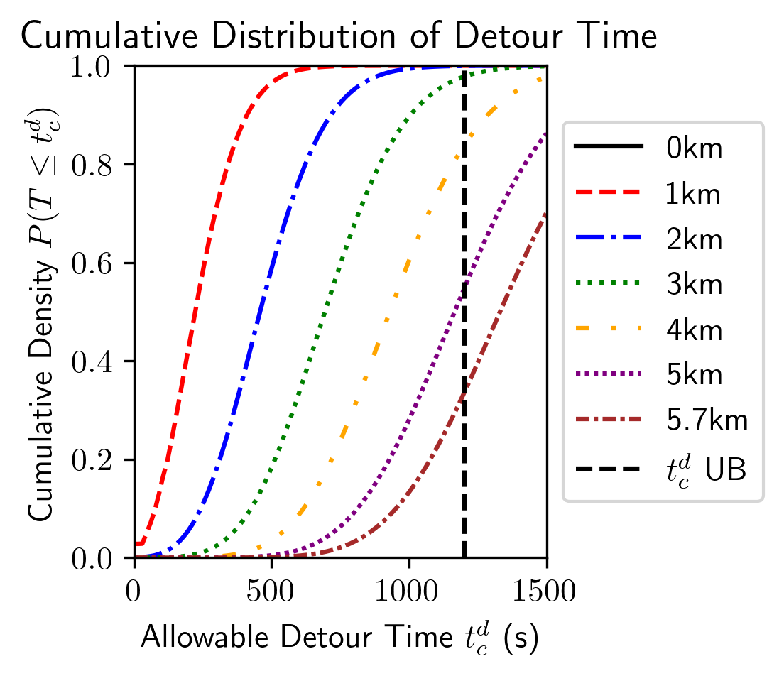
Figure 4: Cumulative distribution of detour time under varying flexible-route portions $x_{f}$ for Route 7 (UB refers to upper bound)

5.2 Simulation of Semi-on-Demand Service

A simulated SoD run of Route 7 is illustrated in Figure 5 as an example. After departing from the Trudering terminus and serving the fixed-route stops (black line), the SAV detours from the original bus route to pick up and drop off passengers in the flexible-route part (blue line). It then returns to the fixed route and terminus.

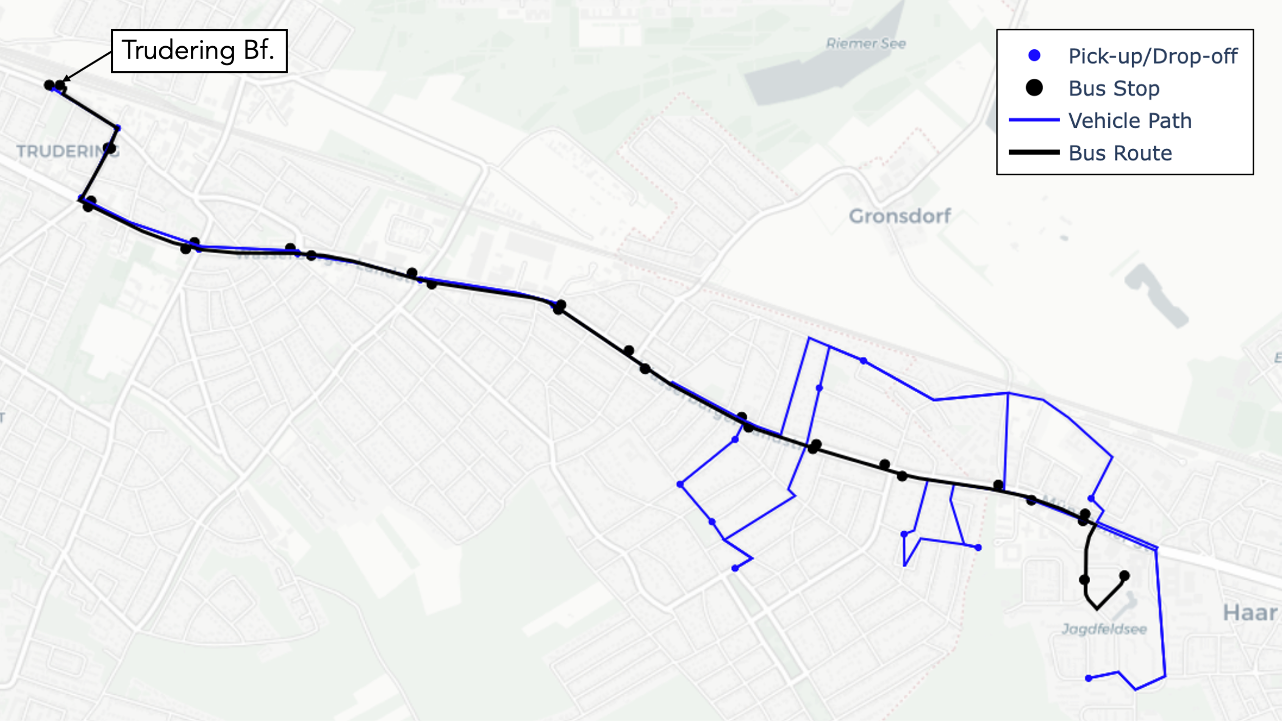
Figure 5: A simulated example of semi-on-demand hybrid route for Route 7

This subsection discusses the simulation results for different routes under varying flexible-route length $x_{f}$. All statistics shown are median values unless otherwise specified.

5.2.1 Full SAV Scenario

Figure 6 shows the different metrics, as a percentage of the SAV fixed-route results ($x_{f}=0$), under varying flexible-route portion $x_{f}$ across the ten routes.

Figure 6: Results under full SAV scenario

The generalized costs shown in Figure 6(a) reveal that some routes (e.g., Routes 2, 8, 10) achieve optimal performance with fully flexible routing, while others (e.g., Routes 1, 3, 5) benefit most from limited flexible-route portions. The savings range from 15% (Route 1) to 50% (Route 4). The differences highlight the balance between detours and improvements in efficiency across different route characteristics. These can be further analyzed from the user’s and operator’s perspectives.

Figure 6(b) shows the journey time changes, which are affected by the reduced access time and increased detours with longer flexible routes, as well as changes in waiting time and savings in fixed stops. For some routes, e.g., Routes 2 and 8, fully flexible routing brings the minimum journey times. Other routes, like Routes 1, 3, and 5, show an initial decrease in journey time followed by a rebound.

For the operating costs in Figure 6(c), longer routes with medium to low demand, like Routes 4 and 5, show lower operating costs, while Routes 1, 7, 10 exhibit higher operating costs, likely due to higher demand and thus higher occupancy per run (all exceeding 7 passengers).

Due to improved accessibility in the flexible route, the number of requests satisfied generally increases as shown in Figure 6(d). 20%-80% more passengers are served. However, for Route 1, this increase is counterbalanced by excessive detours at longer $x_{f}$ (likely related to its higher ridership). As seen in Figure 6(e), up to 65 requests cannot be served when $x_{f}$ exceeds 6km for this route. Meanwhile, for Route 4, flexible-route service gets rid of the circuitous loop, significantly improving efficiency and accessibility (see Figure 3).

Detailed results are presented in Table LABEL:tab:result ($\alpha=0$) after References.

5.2.2 Transition Scenarios with Drivers

Figure 7 shows only Routes 2 and 7 for clarity, illustrating the differences in the transition and full SAV stage. Figure 7(a) shows that the full SAV case satisfies more requests with longer flexible routes due to improved accessibility. However, for the transition scenarios with 75% and 100% drivers, requests satisfied plateau at respectively 5km and 2km flexible-route length. This is attributed to lower headways in the transition scenarios (Table 2), resulting in more passengers per run and consequently more detours. These factors limit the operational capacity of flexible routes, leading to more request rejection.

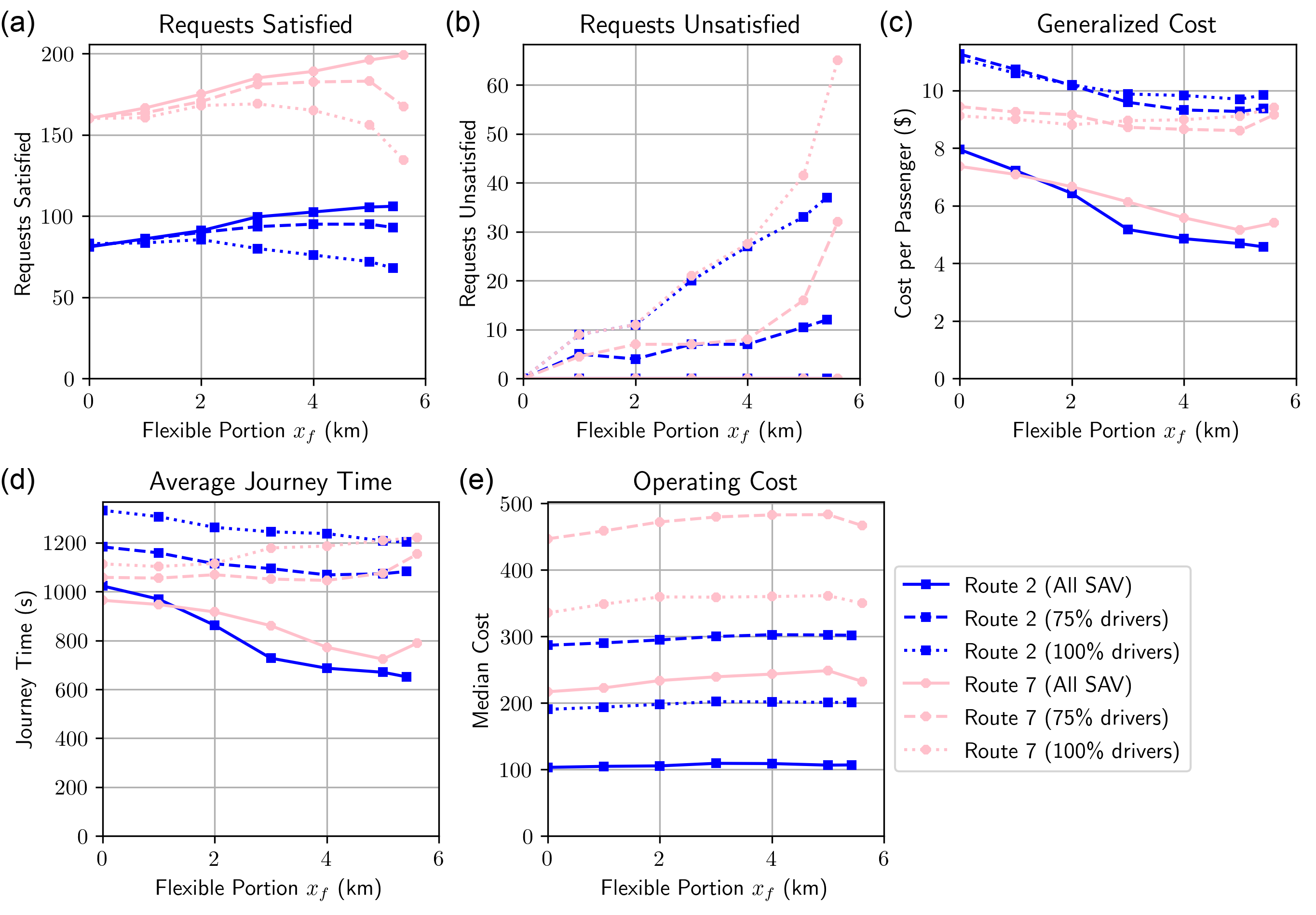
Figure 7: Results under scenarios of full SAV, transition with 75% and 100% drivers

Generalized costs, depicted in Figure 7(c), show that Route 2 still benefits from moderate flexible routing in the transition stage, while the benefits of Route 7 are less visible. In Figure 7(d), the scenarios with more drivers feature higher journey times due to increased waiting times and detours. Besides, these scenarios have higher operating costs due to the labor costs (Figure 7(e)).

Overall, the transition scenarios with drivers limit the SAV benefits in terms of generalized cost reduction and additional passengers served. Nevertheless, adding SAVs parallel to drivers and implementing SoD still offer advantages over existing fixed routes, including increased demand and improved accessibility, particularly at shorter flexible-route portions. The hybrid-route approach provides the flexibility to gradually adjust the flexible-route portion in response to changes in the driver proportion in the fleet.

5.3 Analysis

5.3.1 Use Cases

The implementation and benefits of SoD routes vary significantly across different routes due to specific factors such as demand density and distribution, operating headway, and route length. A clearer trend emerges when we examine the number of riders departing from the terminus per run, as illustrated in Figure 8.

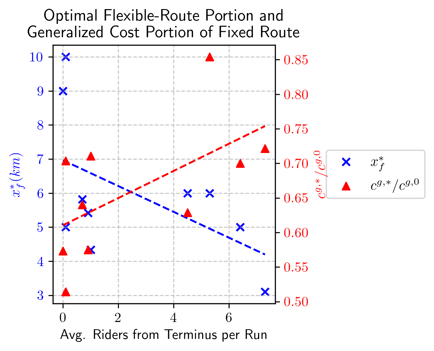
Figure 8: Optimal flexible-route portion and generalized cost portion of fixed route

The figure shows that routes with higher ridership from the terminus per run tend to have shorter optimal flexible-route portions $x_{f}^{*}$ and smaller reductions in generalized cost (higher $c^{g,*}/c^{g,0}$). This pattern may be explained by the better scale of economy of fixed routes under more concentrated demand. Additionally, routes with more passengers per run experience more detours in excessively long flexible routes.

Given the complexity and variability of these factors, it is advisable to utilize the analytical formula (Ng et al. 2024a) and run simulations for each route under various implementation scenarios to determine the optimal strategy.

5.3.2 Comparison with Theoretical Results

Figure 9 illustrates the trade-offs among various passenger time metrics (solid lines) as the flexible-route portion increases, compared with theoretical values assuming a uniform demand distribution (dashed lines) for Route 7.

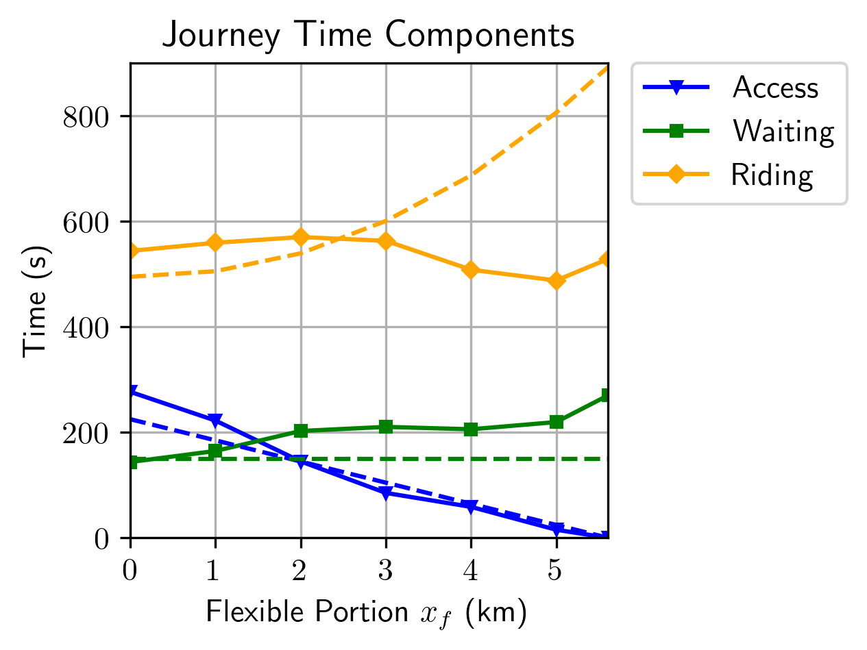
Figure 9: Comparison between results of simulation (solid lines) and theoretical (dashed lines) values of Route 7 (full SAV scenario)

Access (walking) times decrease with longer flexible routes, indicating improved service accessibility that aligns with theoretical predictions. Waiting times increase gradually with $x_{f}$ due to the effects of detours on headway variance. Riding times fluctuate around the same level, contrary to the theoretical quadratic increase, possibly reflecting the limit set by the constraint of the detour factor.

5.3.3 User Experience Analysis

Would SoD routes bring different user experiences for different riders? Figure 10 shows the cumulative distribution of user experiences under varying flexible-route portions $x_{f}$.

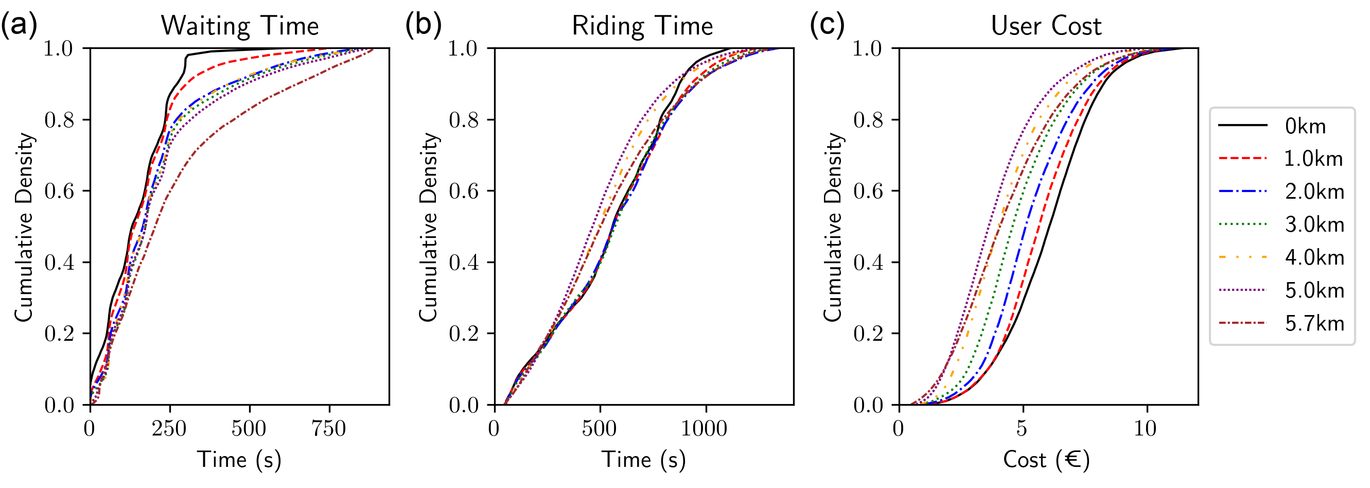
Figure 10: Distribution of user experience under varying flexible-route portions $x_{f}$ of Route 7 (full SAV scenario)

Waiting time changes (Figure 10(a)) reveal that the fixed route (0km) offers the lowest and most consistent waiting times. As the flexible-route portion increases, waiting times gradually rise, with the higher end experiencing considerably longer waiting times (approaching the 15-minute limit). Fully flexible routes perform the worst in terms of waiting time consistency.

In Figure 10(b), riding time decreases slightly with longer flexible routes, likely due to savings in fixed dwell times. However, this effect is relatively modest and evenly distributed across users. Examining overall user cost (access + waiting + riding) in Figure 10(c), we observe a seemingly balanced outcome. Users who benefit from reduced walking distances often experience longer waiting times, particularly at the flexible end of the route. Despite this trade-off, the overall impact appears beneficial for most users.

This example showcases the use of cumulative distribution charts to analyze the variation in user experience implementing SoD service in each route. Other equity metrics (Mahmassani et al. 2024) can provide a more comprehensive picture of its impacts during planning.

6 Conclusion

This study addresses research gaps in semi-on-demand (SoD) service planning, simulation, and analysis with shared autonomous vehicles (SAVs). We focused on improving current transit services by optimizing peak-hour fixed-route operations and implementing off-peak SoD services in the same route catchment area. Our research addresses four key aspects: (i) determining optimal fleet and vehicle sizes for peak-hour fixed-route services with SAVs, (ii) assessing the impact of operating budgets during the transition from human drivers to full automation, (iii) developing optimal service planning for off-peak SoD hybrid-route services in schedule and flexible-route length, and (iv) identifying suitable use cases for off-peak SoD services.

For peak-hour fixed routes, we analytically optimize fleet and vehicle sizes that minimize users’ waiting time and operator’s cost under budget and capacity constraints. Off-peak SoD service is conceptualized with analytical schedule settings and analyzed with an agent-based simulation on ten existing bus routes in Munich, Germany. Results corroborate the SoD benefits, satisfying up to 80% more requests and saving up to 50% generalized cost when using SAVs. At moderate flexible-route lengths, SoD routes avoid excessive detours and attract more demand with the door-to-door convenience. Cross-route comparison and user experience analysis enhance the precision of use case delineation of SoD with SAVs.

Our findings highlight that SAVs can bring considerable benefits in fixed-route service quality through increased frequency and smaller vehicle sizes, even during the transition with a partial or full human driver workforce. The increased fleet size and reduced headways favor more flexible-route operation in the SoD service. In the case study, some routes benefit from fully flexible operations, while others still require some fixed-route portion to avoid excessive detours and operational burden to serve all passengers. During the transition phase, the limited fleet size and higher headway constrain the benefits of flexible-route operations. Nevertheless, SoD hybrid routes offer a good transition strategy, allowing for gradual adjustment of the flexible-route portion when more SAVs are deployed. Notably, for all routes studied, optimal fleet and vehicle sizes with 50% or more SAVs converge to the full SAV solution, indicating that SAV capital cost, rather than day-to-day operating costs, becomes the decision factor in the later stages of transition. Furthermore, our analysis identifies that average occupancy per run from the terminus, among other demand and operational characteristics, is an important factor in determining the benefits of SoD.

We also highlight several limitations in this study for further research:

• Cross-line effects, including demand and fleet assignment across multiple routes, call for more holistic optimization.

• The interaction between SoD services and ride-pooling/ride-sharing systems may offer synergy or competition.

• Further optimization of headway settings could enhance the efficiency of SoD operations.

• The feasibility of larger SAVs navigating residential areas for pick-up and drop-off needs further investigation, although smaller vehicles are expected with full SAV deployment.

In conclusion, this study demonstrates the potential of SoD hybrid-route services using SAVs to enhance public transit systems with higher efficiency and better accessibility. The step-by-step service planning, operational simulation, and analysis framework, coupled with previous theoretical approach (Ng et al. 2024a), supports transit agencies in planning and evaluating the strategy to roll out SoD services with SAVs in existing networks.

Simulation Result Table

Table LABEL:tab:result shows the simulation results discussed in Section 5.2. All metrics shown are median values. $\alpha=0.75$ case is not shown if equivalent to $\alpha=0$.

Table 3: Simulation Results

Route	$\alpha$	$x_{f}$ (km)	Requests	Requests satisfied	Avg. Time (s)				Veh. dist. (km)	Avg. gen. cost (€)
					Ride	Wait	Walk	Journey
1	0	0.0	291	291	10.21	2.44	5.21	17.89	773.1	9.35
1	0	1.0	301	301	10.53	2.55	4.42	17.51	777.0	8.96
1	0	2.0	302	302	10.32	2.82	4.27	17.46	785.8	8.97
1	0	3.0	307	307	9.95	3.18	3.95	17.15	796.8	8.83
1	0	4.0	320	320	9.55	3.75	2.96	16.32	808.0	8.31
1	0	5.0	323	323	9.32	4.12	2.71	16.11	805.1	8.22
1	0	6.0	334	334	9.65	4.48	1.98	15.96	810.3	7.99
1	0	7.0	354	336	10.51	5.65	1.29	17.46	822.9	8.38
1	0	8.0	359.5	341.5	10.47	6.02	0.79	17.22	830.8	8.19
1	0	9.0	369	345	10.64	6.59	0.17	17.41	842.0	8.18
1	0	9.9	372	307	11.63	7.86	0.00	19.52	816.1	9.07
1	1	0.0	291	291	10.21	2.44	5.21	17.89	1391.1	11.47
1	1	1.0	301	301	10.53	2.55	4.42	17.51	1395.0	11.03
1	1	2.0	302	302	10.32	2.82	4.27	17.46	1403.8	11.02
1	1	3.0	307	307	9.95	3.18	3.95	17.15	1414.8	10.83
1	1	4.0	320	320	9.55	3.75	2.96	16.32	1426.0	10.22
1	1	5.0	323	323	9.32	4.12	2.71	16.11	1423.1	10.14
1	1	6.0	334	334	9.65	4.48	1.98	15.96	1428.3	9.85
1	1	7.0	354	336	10.51	5.65	1.29	17.46	1440.9	10.22
1	1	8.0	359.5	341.5	10.47	6.02	0.79	17.22	1448.8	10.04
1	1	9.0	369	345	10.64	6.59	0.17	17.41	1460.0	9.97
1	1	9.9	372	307	11.63	7.86	0.00	19.52	1434.1	11.09
2	0	0.0	81	81	8.97	1.96	6.17	17.05	103.3	7.95
2	0	1.0	86	86	9.05	2.58	4.38	16.15	104.8	7.22
2	0	2.0	91	91	8.36	2.63	3.44	14.37	105.5	6.43
2	0	3.0	99.5	99.5	7.99	2.82	1.32	12.13	109.3	5.17
2	0	4.0	102.5	102.5	7.34	3.40	0.69	11.44	108.9	4.86
2	0	5.0	105.5	105.5	7.00	4.15	0.05	11.17	106.6	4.68
2	0	5.4	106	106	6.80	4.03	0.00	10.86	106.9	4.57
2	0.75	0.0	81.5	81.5	9.08	4.46	6.11	19.72	286.7	11.26
2	0.75	1.0	92	85.5	9.49	5.36	4.49	19.31	290.3	10.73
2	0.75	2.0	94.5	90	9.31	5.70	3.52	18.56	294.7	10.18
2	0.75	3.0	101	93.5	9.81	7.06	1.42	18.23	299.9	9.59
2	0.75	4.0	103.5	95	9.41	7.66	0.70	17.81	302.6	9.32
2	0.75	5.0	106	95	9.13	8.46	0.05	17.88	302.2	9.27
2	0.75	5.4	106	93	9.18	8.66	0.00	18.04	301.8	9.38
2	1	0.0	83	83	9.06	7.01	6.19	22.21	190.4	11.10
2	1	1.0	93	83.5	9.75	7.50	4.49	21.78	193.8	10.60
2	1	2.0	96	85.5	9.92	7.67	3.58	21.05	198.0	10.20
2	1	3.0	101	80	10.47	8.87	1.54	20.74	202.0	9.88
2	1	4.0	104.5	76	10.37	9.43	0.84	20.62	201.6	9.83
2	1	5.0	106	72	9.78	10.11	0.07	20.12	200.9	9.70
2	1	5.4	106	68	9.84	10.22	0.00	20.05	200.9	9.84
3	0	0.0	91.5	91.5	10.86	1.86	6.97	19.68	578.6	13.85
3	0	1.0	96.5	96.5	11.06	2.13	5.74	18.83	578.1	13.11
3	0	2.0	99	99	10.87	2.08	5.13	18.12	577.9	12.53
3	0	3.0	102	102	9.98	2.16	4.58	16.66	578.6	11.86
3	0	4.0	103.5	103.5	9.08	2.39	4.07	15.58	579.6	11.27
3	0	5.0	116	116	9.12	3.66	1.26	14.14	584.8	9.75
3	0	6.0	118	118	9.46	4.81	0.81	15.05	579.8	9.98
3	0	7.0	120.5	120.5	9.73	5.59	0.44	15.86	580.2	10.04
3	0	8.0	122	122	9.89	6.11	0.00	15.85	581.6	9.96
3	0	9.0	122	122	10.06	6.69	0.00	16.76	578.1	10.25
3	0	10.0	122.5	122.5	10.56	7.62	0.00	18.37	571.0	10.74
3	0	10.7	122	122	10.37	7.54	0.00	17.98	573.5	10.64
3	0.75	0.0	91.5	91.5	10.86	1.86	6.97	19.68	2087.8	30.30
3	0.75	1.0	96	96	11.04	2.13	5.74	18.81	2086.9	28.73
3	0.75	2.0	99	99	10.87	2.09	5.13	18.13	2086.6	27.78
3	0.75	3.0	102	102	9.98	2.15	4.57	16.66	2087.7	26.69
3	0.75	4.0	103.5	103.5	9.15	2.42	4.06	15.58	2089.3	25.88
3	0.75	5.0	116	116	9.06	3.62	1.28	14.13	2097.8	22.82
3	0.75	6.0	118	118	9.43	4.75	0.81	15.00	2089.6	22.82
3	0.75	7.0	120.5	120.5	9.76	5.54	0.44	15.73	2090.6	22.58
3	0.75	8.0	122	122	9.92	6.06	0.00	15.95	2092.0	22.30
3	0.75	9.0	122	122	10.19	6.66	0.00	16.89	2086.4	22.61
3	0.75	10.0	122.5	122.5	10.67	7.53	0.00	18.14	2074.8	22.93
3	0.75	10.7	122	122	10.42	7.54	0.00	18.04	2079.1	22.97
3	1	0.0	91.5	91.5	10.86	1.86	6.97	19.68	1590.4	24.89
3	1	1.0	96	96	11.04	2.13	5.74	18.81	1589.5	23.57
3	1	2.0	99	99	10.87	2.09	5.13	18.13	1589.2	22.73
3	1	3.0	102	102	9.98	2.15	4.57	16.66	1590.3	21.80
3	1	4.0	103.5	103.5	9.15	2.42	4.06	15.58	1591.9	21.07
3	1	5.0	116	116	9.06	3.62	1.28	14.13	1600.4	18.50
3	1	6.0	118	118	9.43	4.75	0.81	15.00	1592.2	18.60
3	1	7.0	120.5	120.5	9.76	5.54	0.44	15.73	1593.2	18.45
3	1	8.0	122	122	9.92	6.06	0.00	15.95	1594.6	18.25
3	1	9.0	122	122	10.19	6.66	0.00	16.89	1589.0	18.56
3	1	10.0	122.5	122.5	10.67	7.53	0.00	18.14	1577.4	18.86
3	1	10.7	122	122	10.42	7.54	0.00	18.04	1581.7	18.83
4	0	0.0	16	16	10.12	4.21	5.83	20.42	149.1	17.38
4	0	1.0	17.5	17.5	9.92	4.36	5.52	19.75	147.0	16.05
4	0	2.0	19	19	9.63	4.35	5.41	19.34	145.8	15.28
4	0	3.0	22	22	8.52	4.49	4.91	18.07	147.6	13.64
4	0	4.0	23	23	8.66	4.08	4.07	17.15	146.9	12.72
4	0	5.0	24.5	24.5	9.40	3.84	3.78	17.17	145.8	12.22
4	0	6.0	25.5	25.5	9.15	3.39	2.97	15.85	144.3	11.26
4	0	7.0	27	27	8.28	3.81	2.10	14.33	143.9	10.40
4	0	8.0	27.5	27.5	7.21	4.62	1.53	13.55	143.5	10.13
4	0	9.0	29	29	6.70	5.31	0.95	12.99	142.6	9.56
4	0	10.0	30	30	6.33	5.42	0.22	11.95	142.0	8.94
4	0	11.0	30	30	6.68	6.09	0.00	12.67	141.1	9.01
4	0	11.9	30	30	6.55	6.35	0.00	12.98	140.4	9.24
4	0.75	0.0	16	16	10.12	4.21	5.83	20.39	922.7	66.52
4	0.75	1.0	17.5	17.5	9.92	4.36	5.52	19.75	920.2	60.11
4	0.75	2.0	19	19	9.63	4.35	5.41	19.34	918.7	56.89
4	0.75	3.0	22	22	8.52	4.49	4.91	18.07	920.8	48.97
4	0.75	4.0	23	23	8.66	4.08	4.07	17.15	920.0	46.08
4	0.75	5.0	24.5	24.5	9.40	3.84	3.78	17.17	918.6	43.81
4	0.75	6.0	25.5	25.5	9.15	3.41	3.00	15.85	916.8	41.75
4	0.75	7.0	27	27	8.28	3.81	2.10	14.29	916.2	39.48
4	0.75	8.0	27.5	27.5	7.21	4.63	1.53	13.59	915.8	38.23
4	0.75	9.0	29	29	6.69	5.28	0.95	12.90	914.7	36.13
4	0.75	10.0	30	30	6.33	5.41	0.22	11.95	914.0	35.11
4	0.75	11.0	30	30	6.68	6.18	0.00	12.73	912.8	34.97
4	0.75	11.9	30	30	6.51	6.36	0.00	13.03	911.9	34.99
4	1	0.0	16	16	10.12	4.21	5.83	20.39	769.1	56.92
4	1	1.0	17.5	17.5	9.92	4.36	5.52	19.75	766.6	51.33
4	1	2.0	19	19	9.63	4.35	5.41	19.34	765.1	48.81
4	1	3.0	22	22	8.52	4.49	4.91	18.07	767.2	41.99
4	1	4.0	23	23	8.66	4.08	4.07	17.15	766.4	39.40
4	1	5.0	24.5	24.5	9.40	3.84	3.78	17.17	765.0	37.53
4	1	6.0	25.5	25.5	9.15	3.41	3.00	15.85	763.2	35.73
4	1	7.0	27	27	8.28	3.81	2.10	14.29	762.6	33.74
4	1	8.0	27.5	27.5	7.21	4.63	1.53	13.59	762.2	32.64
4	1	9.0	29	29	6.69	5.28	0.95	12.90	761.1	30.92
4	1	10.0	30	30	6.33	5.41	0.22	11.95	760.4	29.90
4	1	11.0	30	30	6.68	6.18	0.00	12.73	759.2	29.85
4	1	11.9	30	30	6.51	6.36	0.00	13.03	758.3	29.87
5	0	0.0	97	97	7.51	0.98	6.46	14.87	404.1	10.17
5	0	1.0	98.5	98.5	7.42	1.04	5.96	14.47	392.9	9.74
5	0	2.0	102	102	7.40	1.04	5.53	13.93	384.4	9.27
5	0	3.0	102	102	6.98	1.22	5.13	13.28	381.0	8.98
5	0	4.0	104	104	6.45	1.36	4.84	12.64	376.2	8.55
5	0	5.0	105.5	105.5	6.21	1.54	4.69	12.58	372.3	8.47
5	0	6.0	106	106	5.96	1.67	4.35	12.02	359.6	8.13
5	0	7.0	116.5	116.5	6.46	2.11	2.38	10.99	355.8	7.05
5	0	8.0	120	120	6.04	2.24	1.52	9.81	357.2	6.40
5	0	9.0	125	125	5.56	2.64	0.60	8.83	356.5	5.83
5	0	10.0	127	127	6.15	3.72	0.07	9.93	351.3	6.06
5	0	11.0	126	126	6.48	4.97	0.00	11.38	352.1	6.64
5	0	11.5	128	128	6.51	5.02	0.00	11.56	351.2	6.62
5	0.75	0.0	97	97	7.52	2.10	6.45	16.04	1256.2	19.37
5	0.75	1.0	99	99	7.43	2.10	5.97	15.48	1246.1	18.87
5	0.75	2.0	101.5	101.5	7.46	2.05	5.50	15.05	1239.2	18.10
5	0.75	3.0	102.5	102.5	7.07	2.18	5.09	14.31	1238.0	17.75
5	0.75	4.0	105.5	105.5	6.52	2.26	4.84	13.63	1234.6	17.11
5	0.75	5.0	104	104	6.29	2.40	4.66	13.49	1232.1	17.12
5	0.75	6.0	106	106	6.11	2.51	4.34	13.05	1221.1	16.68
5	0.75	7.0	117	117	6.75	2.85	2.38	11.98	1222.5	14.89
5	0.75	8.0	121	121	6.47	3.01	1.49	10.93	1227.6	14.08
5	0.75	9.0	126	126	5.72	2.99	0.59	9.37	1232.2	12.93
5	0.75	10.0	127.5	127.5	6.14	3.69	0.07	9.89	1230.8	12.83
5	0.75	11.0	127.5	127.5	6.56	4.77	0.00	11.31	1226.9	13.37
5	0.75	11.5	127	127	6.52	4.74	0.00	11.23	1224.6	13.41
5	1	0.0	97	97	7.52	2.10	6.45	16.04	1206.6	18.87
5	1	1.0	99	99	7.43	2.10	5.97	15.48	1196.5	18.35
5	1	2.0	101.5	101.5	7.46	2.05	5.50	15.05	1189.6	17.62
5	1	3.0	102.5	102.5	7.07	2.18	5.09	14.31	1188.4	17.27
5	1	4.0	105.5	105.5	6.52	2.26	4.84	13.63	1185.0	16.64
5	1	5.0	104	104	6.29	2.40	4.66	13.49	1182.5	16.65
5	1	6.0	106	106	6.11	2.51	4.34	13.05	1171.5	16.21
5	1	7.0	117	117	6.75	2.85	2.38	11.98	1172.9	14.45
5	1	8.0	121	121	6.47	3.01	1.49	10.93	1178.0	13.67
5	1	9.0	126	126	5.72	2.99	0.59	9.37	1182.6	12.54
5	1	10.0	127.5	127.5	6.14	3.69	0.07	9.89	1181.2	12.45
5	1	11.0	127.5	127.5	6.56	4.77	0.00	11.31	1177.3	12.98
5	1	11.5	127	127	6.52	4.74	0.00	11.23	1175.0	13.02
6	0	0.0	129	129	7.17	2.58	4.99	14.65	269.1	7.84
6	0	1.0	143	143	7.41	3.28	3.71	14.50	273.3	7.39
6	0	2.0	150	150	7.30	3.62	3.22	14.23	277.0	7.17
6	0	3.0	153	153	7.35	3.64	2.60	13.62	275.2	6.76
6	0	4.0	157	157	7.14	3.74	1.97	12.94	273.6	6.33
6	0	5.0	165	165	6.71	3.55	0.99	11.26	272.6	5.52
6	0	6.0	172	172	6.61	3.28	0.26	10.11	278.1	4.93
6	0	6.8	171.5	171.5	7.14	4.28	0.00	11.41	272.9	5.30
6	1	0.0	129	129	7.23	3.11	4.94	15.30	571.2	10.44
6	1	1.0	140	140	7.44	4.33	3.72	15.48	579.5	9.97
6	1	2.0	148	148	7.56	4.57	3.26	15.53	585.5	9.71
6	1	3.0	153	153	7.43	4.21	2.61	14.29	585.2	9.07
6	1	4.0	157	157	7.21	4.51	1.99	13.69	584.4	8.65
6	1	5.0	164	164	6.95	4.37	1.02	12.30	585.0	7.82
6	1	6.0	171	171	7.06	4.58	0.25	11.79	590.5	7.38
6	1	6.8	174	168	7.98	5.65	0.00	13.58	582.6	8.03
7	0	0.0	160	160	9.07	2.40	4.61	16.07	216.9	7.36
7	0	1.0	166.5	166.5	9.32	2.75	3.71	15.79	222.7	7.09
7	0	2.0	175	175	9.51	3.38	2.42	15.28	233.7	6.66
7	0	3.0	185	185	9.39	3.51	1.42	14.35	239.3	6.13
7	0	4.0	189	189	8.47	3.43	0.98	12.87	243.4	5.58
7	0	5.0	196	196	8.13	3.66	0.26	12.06	248.6	5.16
7	0	5.6	199	199	8.82	4.51	0.00	13.15	232.3	5.40
7	0.75	0.0	160.5	160.5	9.18	3.86	4.62	17.64	446.7	9.44
7	0.75	1.0	169	163.5	9.33	4.52	3.72	17.59	458.5	9.25
7	0.75	2.0	178	170.5	9.51	5.73	2.49	17.82	472.1	9.16
7	0.75	3.0	188	181	9.96	6.12	1.46	17.52	479.5	8.72
7	0.75	4.0	192	182.5	9.87	6.58	0.99	17.43	482.6	8.65
7	0.75	5.0	199	183	10.46	7.13	0.28	17.93	483.0	8.61
7	0.75	5.6	200	167.5	11.23	7.99	0.00	19.22	466.5	9.16
7	1	0.0	160	160	9.23	4.74	4.59	18.56	335.3	9.12
7	1	1.0	170	160.5	9.05	5.50	3.76	18.38	348.5	9.00
7	1	2.0	180	168	9.63	6.35	2.50	18.59	359.3	8.81
7	1	3.0	190	169	10.77	7.30	1.52	19.65	359.0	8.95
7	1	4.0	195	165	10.79	7.83	1.05	19.77	360.0	8.98
7	1	5.0	200	156	11.18	8.63	0.31	20.16	361.2	9.11
7	1	5.6	200	134.5	11.53	8.84	0.00	20.35	349.8	9.40
8	0	0.0	34	34	8.48	4.97	7.05	20.45	273.1	16.29
8	0	1.0	35	35	8.36	4.89	6.27	19.63	272.1	15.73
8	0	2.0	35	35	8.41	4.69	6.12	19.40	274.0	15.46
8	0	3.0	35	35	7.38	3.72	5.34	16.35	273.4	14.28
8	0	4.0	37	37	6.67	3.49	4.21	14.38	272.8	13.06
8	0	4.3	39	39	6.38	3.43	2.16	12.12	274.3	11.57
8	1	0.0	34	34	8.48	4.97	7.05	20.45	813.7	32.16
8	1	1.0	35	35	8.36	4.89	6.27	19.63	812.1	31.22
8	1	2.0	35	35	8.41	4.69	6.12	19.40	815.1	30.99
8	1	3.0	35	35	7.38	3.72	5.34	16.35	814.2	29.31
8	1	4.0	37	37	6.67	3.49	4.21	14.38	813.2	27.58
8	1	4.3	39	39	6.38	3.43	2.16	12.12	815.6	25.34
9	0	0.0	52	52	7.73	3.93	4.86	16.56	228.0	10.72
9	0	1.0	53	53	7.93	4.08	4.09	16.11	227.2	10.32
9	0	2.0	55.5	55.5	7.60	4.18	3.53	15.22	228.3	9.80
9	0	3.0	56	56	6.54	3.60	2.80	13.04	228.4	8.87
9	0	4.0	58	58	5.95	3.41	1.75	11.12	227.8	7.94
9	0	5.0	60	60	6.31	3.97	0.31	10.51	227.6	7.33
9	0	5.8	61	61	6.18	3.48	0.00	9.60	227.8	6.86
9	0.75	0.0	52	52	7.76	3.79	4.86	16.41	1136.6	28.23
9	0.75	1.0	53	53	7.95	3.96	4.09	15.98	1135.7	27.29
9	0.75	2.0	55.5	55.5	7.62	4.08	3.53	15.20	1137.0	26.09
9	0.75	3.0	56.5	56.5	6.46	3.61	2.82	12.95	1137.0	25.00
9	0.75	4.0	58	58	5.94	3.37	1.75	11.13	1136.3	23.50
9	0.75	5.0	60	60	6.28	3.96	0.32	10.51	1135.9	22.46
9	0.75	5.8	61	61	6.18	3.40	0.00	9.57	1136.2	21.91
9	1	0.0	52	52	7.76	3.79	4.86	16.41	600.4	17.85
9	1	1.0	53	53	7.95	3.96	4.09	15.98	599.1	17.32
9	1	2.0	55.5	55.5	7.62	4.08	3.53	15.20	601.1	16.46
9	1	3.0	56.5	56.5	6.46	3.61	2.82	12.95	601.1	15.45
9	1	4.0	58	58	5.94	3.37	1.75	11.13	600.1	14.20
9	1	5.0	60	60	6.28	3.96	0.32	10.51	599.4	13.53
9	1	5.8	61	61	6.18	3.40	0.00	9.57	599.9	13.08
10	0	0.0	74	74	5.77	4.20	3.07	13.02	68.2	5.95
10	0	1.0	77	77	6.42	4.02	1.75	12.19	76.6	5.35
10	0	2.0	80	80	5.91	3.54	0.90	10.37	78.0	4.57
10	0	3.0	83	83	6.93	3.62	0.11	10.78	74.3	4.39
10	0	3.1	83	83	6.96	3.75	0.00	10.64	74.4	4.30
10	1	0.0	74	74	5.80	5.29	3.09	14.08	188.0	8.00
10	1	1.0	78	78	6.67	4.95	1.76	13.44	196.2	7.38
10	1	2.0	80	80	6.01	3.78	0.91	10.73	199.4	6.22
10	1	3.0	81	81	7.32	4.13	0.11	11.43	195.9	6.22
10	1	3.1	82.5	82.5	7.40	4.50	0.00	11.91	196.1	6.25

References

- Alonso-Mora et al. (2017) Alonso-Mora, J., Samaranayake, S., Wallar, A., Frazzoli, E., Rus, D., 2017. On-demand high-capacity ride-sharing via dynamic trip-vehicle assignment. Proceedings of the National Academy of Sciences 114, 462–467. doi:doi:10.1073/pnas.1611675114.
- Armellini (2021) Armellini, M.G., 2021. A Tool for Simulating Demand Responsive Transport Systems in SUMO, in: 2021 7th International Conference on Models and Technologies for Intelligent Transportation Systems (MT-ITS), pp. 1–5. doi:doi:10.1109/MT-ITS49943.2021.9529311.
- Badia and Jenelius (2021) Badia, H., Jenelius, E., 2021. Design and operation of feeder systems in the era of automated and electric buses. Transportation Research Part A: Policy and Practice 152, 146–172. URL: https://www.sciencedirect.com/science/article/pii/S096585642100197X, doi:doi:10.1016/j.tra.2021.07.015.
- Boeing (2017) Boeing, G., 2017. OSMnx: New methods for acquiring, constructing, analyzing, and visualizing complex street networks. Computers, Environment and Urban Systems 65, 126–139. doi:doi:10.1016/j.compenvurbsys.2017.05.004.
- Bösch et al. (2018) Bösch, P.M., Becker, F., Becker, H., Axhausen, K.W., 2018. Cost-based analysis of autonomous mobility services. Transport Policy 64, 76–91. URL: https://www.sciencedirect.com/science/article/pii/S0967070X17300811, doi:doi:10.1016/j.tranpol.2017.09.005.
- Calabrò et al. (2023) Calabrò, G., Araldo, A., Oh, S., Seshadri, R., Inturri, G., Ben-Akiva, M., 2023. Adaptive transit design: Optimizing fixed and demand responsive multi-modal transportation via continuous approximation. Transportation Research Part A: Policy and Practice 171, 103643. URL: https://www.sciencedirect.com/science/article/pii/S0965856423000630, doi:doi:10.1016/j.tra.2023.103643.
- Cao and Ceder (2019) Cao, Z., Ceder, A., 2019. Autonomous shuttle bus service timetabling and vehicle scheduling using skip-stop tactic. Transportation Research Part C: Emerging Technologies 102, 370–395. URL: https://www.sciencedirect.com/science/article/pii/S0968090X18309744, doi:doi:10.1016/j.trc.2019.03.018.
- Chen and Nie (2017) Chen, P.W., Nie, Y.M., 2017. Analysis of an idealized system of demand adaptive paired-line hybrid transit. Transportation Research Part B: Methodological 102, 38–54. URL: http://www.sciencedirect.com/science/article/pii/S0191261516305562, doi:doi:10.1016/j.trb.2017.05.004.
- Cokyasar et al. (2022) Cokyasar, T., de Souza, F., Auld, J., Verbas, O., 2022. Dynamic Ride-Matching for Large-Scale Transportation Systems. Transportation Research Record 2676, 172–182. doi:doi:10.1177/03611981211049422.
- Cortina et al. (2023) Cortina, M., Chiabaut, N., Leclercq, L., 2023. Fostering synergy between transit and Autonomous Mobility-on-Demand systems: A dynamic modeling approach for the morning commute problem. Transportation Research Part A: Policy and Practice 170, 103638. URL: https://linkinghub.elsevier.com/retrieve/pii/S0965856423000587, doi:doi:10.1016/j.tra.2023.103638.
- Dandl et al. (2021) Dandl, F., Engelhardt, R., Hyland, M., Tilg, G., Bogenberger, K., Mahmassani, H.S., 2021. Regulating mobility-on-demand services: Tri-level model and Bayesian optimization solution approach. Transportation Research Part C: Emerging Technologies 125, 103075. doi:doi:10.1016/j.trc.2021.103075.
- Dandl et al. (2019) Dandl, F., Hyland, M., Bogenberger, K., Mahmassani, H.S., 2019. Evaluating the impact of spatio-temporal demand forecast aggregation on the operational performance of shared autonomous mobility fleets. Transportation 46, 1975–1996. doi:doi:10.1007/s11116-019-10007-9.
- Engelhardt and Bogenberger (2021) Engelhardt, R., Bogenberger, K., 2021. Benefits of flexible boarding locations in on-demand ride-pooling systems, in: 2021 7th International Conference on Models and Technologies for Intelligent Transportation Systems (MT-ITS), IEEE. pp. 1–6. doi:doi:10.1109/MT-ITS49943.2021.9529284.
- Engelhardt et al. (2022) Engelhardt, R., Dandl, F., Syed, A.A., Zhang, Y., Fehn, F., Wolf, F., Bogenberger, K., 2022. FleetPy: A Modular Open-Source Simulation Tool for Mobility On-Demand Services. doi:doi:10.48550/arXiv.2207.14246.
- Engelhardt et al. (2024) Engelhardt, R., Mahmassani, H.S., Bogenberger, K., 2024. Predictive vehicle repositioning for on-demand ride-pooling services, in: 103rd Transportation Research Board Annual Meeting. URL: http://arxiv.org/pdf/2308.05507v1.
- Errico et al. (2013) Errico, F., Crainic, T.G., Malucelli, F., Nonato, M., 2013. A survey on planning semi-flexible transit systems: Methodological issues and a unifying framework. Transportation Research Part C: Emerging Technologies 36, 324–338. doi:doi:10.1016/j.trc.2013.08.010.
- Fagnant and Kockelman (2018) Fagnant, D.J., Kockelman, K.M., 2018. Dynamic ride-sharing and fleet sizing for a system of shared autonomous vehicles in Austin, Texas. Transportation 45, 143–158. doi:doi:10.1007/s11116-016-9729-z.
- Fielbaum et al. (2021) Fielbaum, A., Bai, X., Alonso-Mora, J., 2021. On-demand ridesharing with optimized pick-up and drop-off walking locations. Transportation Research Part C: Emerging Technologies 126, 103061. URL: https://www.sciencedirect.com/science/article/pii/S0968090X21000887, doi:doi:10.1016/j.trc.2021.103061.
- Frei et al. (2017) Frei, C., Hyland, M., Mahmassani, H.S., 2017. Flexing service schedules: Assessing the potential for demand-adaptive hybrid transit via a stated preference approach. Transportation Research Part C: Emerging Technologies 76, 71–89. URL: https://www.sciencedirect.com/science/article/pii/S0968090X1630273X, doi:doi:10.1016/j.trc.2016.12.017.
- Galarza Montenegro et al. (2021) Galarza Montenegro, B.D., Sörensen, K., Vansteenwegen, P., 2021. A large neighborhood search algorithm to optimize a demand-responsive feeder service. Transportation Research Part C: Emerging Technologies 127, 103102. URL: https://www.sciencedirect.com/science/article/pii/S0968090X21001236, doi:doi:10.1016/j.trc.2021.103102.
- Gurumurthy et al. (2020a) Gurumurthy, K.M., Kockelman, K.M., Zuniga-Garcia, N., 2020a. First-Mile-Last-Mile Collector-Distributor System using Shared Autonomous Mobility. Transportation Research Record 2674, 638–647. URL: https://doi.org/10.1177/0361198120936267, doi:doi:10.1177/0361198120936267. publisher: SAGE Publications Inc.
- Gurumurthy et al. (2020b) Gurumurthy, K.M., de Souza, F., Enam, A., Auld, J., 2020b. Integrating Supply and Demand Perspectives for a Large-Scale Simulation of Shared Autonomous Vehicles. Transportation Research Record 2674, 181–192. doi:doi:10.1177/0361198120921157.
- Gurumurthy et al. (2020c) Gurumurthy, K.M., de Souza, F., Enam, A., Auld, J., 2020c. Integrating supply and demand perspectives for a large-scale simulation of shared autonomous vehicles. Transportation Research Record: Journal of the Transportation Research Board 2674, 181–192. doi:doi:10.1177/0361198120921157.
- Hatzenbühler et al. (2020) Hatzenbühler, J., Cats, O., Jenelius, E., 2020. Transitioning towards the deployment of line-based autonomous buses: Consequences for service frequency and vehicle capacity. Transportation Research Part A: Policy and Practice 138, 491–507. URL: https://www.sciencedirect.com/science/article/pii/S0965856420306388, doi:doi:10.1016/j.tra.2020.06.019.
- Horni et al. (2016) Horni, A., Nagel, K., Axhausen, K.W., 2016. The Multi-Agent Transport Simulation MATSim. Ubiquity Press. doi:doi:10.5334/baw.
- Johnson et al. (1995) Johnson, N.L., Kotz, S., Balakrishnan, N., 1995. Continuous univariate distributions, volume 2. volume 289. John wiley & sons.
- Levin et al. (2019) Levin, M.W., Odell, M., Samarasena, S., Schwartz, A., 2019. A linear program for optimal integration of shared autonomous vehicles with public transit. Transportation Research Part C: Emerging Technologies 109, 267–288. URL: http://www.sciencedirect.com/science/article/pii/S0968090X19314445, doi:doi:10.1016/j.trc.2019.10.007.
- Li et al. (2023) Li, M., Lee, E., Lo, H.K., 2023. Frequency-based zonal flexible bus design considering order cancellation. Transportation Research Part C: Emerging Technologies 152, 104171. URL: https://www.sciencedirect.com/science/article/pii/S0968090X23001602, doi:doi:10.1016/j.trc.2023.104171.
- Li and Quadrifoglio (2010) Li, X., Quadrifoglio, L., 2010. Feeder transit services: Choosing between fixed and demand responsive policy. Transportation Research Part C: Emerging Technologies 18, 770–780. URL: https://www.sciencedirect.com/science/article/pii/S0968090X09000801, doi:doi:10.1016/j.trc.2009.05.015.
- Mahmassani et al. (2024) Mahmassani, H., Raymer, M., Ng, M., 2024. Improving Equity: Public Transit Network Redesign with Shared Autonomous Mobility, in: IPAM Mathematical Foundations for Equity in Transportation Systems Workshop, Los Angeles, CA. URL: https://helper.ipam.ucla.edu/publications/fis2024/fis2024_19820.pdf.
- Masoud and Jayakrishnan (2017) Masoud, N., Jayakrishnan, R., 2017. A decomposition algorithm to solve the multi-hop peer-to-peer ride-matching problem. Transportation Research Part B: Methodological 99, 1–29. URL: https://www.sciencedirect.com/science/article/pii/S019126151730019X, doi:doi:10.1016/j.trb.2017.01.004.
- Moeckel et al. (2020) Moeckel, R., Kuehnel, N., Llorca, C., Moreno, A.T., Rayaprolu, H., 2020. Agent-Based Simulation to Improve Policy Sensitivity of Trip-Based Models. Journal of Advanced Transportation 2020, 1902162. URL: https://onlinelibrary.wiley.com/doi/abs/10.1155/2020/1902162, doi:doi:10.1155/2020/1902162.
- MVG (2024) MVG, 2024. MVG timetable data in GTFS format. URL: https://www.mvg.de/services/fahrgastservice/fahrplandaten.html[Accessed:2024-01-26].
- Namdarpour et al. (2024) Namdarpour, F., Liu, B., Kuehnel, N., Zwick, F., Chow, J.Y., 2024. On non-myopic internal transfers in large-scale ride-pooling systems. Transportation Research Part C: Emerging Technologies 162, 104597. URL: https://www.sciencedirect.com/science/article/pii/S0968090X24001189, doi:doi:10.1016/j.trc.2024.104597.
- Narayanan et al. (2020) Narayanan, S., Chaniotakis, E., Antoniou, C., 2020. Shared autonomous vehicle services: A comprehensive review. Transportation Research Part C: Emerging Technologies 111, 255–293. doi:doi:10.1016/j.trc.2019.12.008.
- Newell (1979) Newell, G.F., 1979. Some Issues Relating to the Optimal Design of Bus Routes. Transportation Science 13, 20–35. URL: http://pubsonline.informs.org/doi/abs/10.1287/trsc.13.1.20, doi:doi:10.1287/trsc.13.1.20.
- Ng et al. (2024a) Ng, M.T.M., Dandl, F., Mahmassani, H.S., Bogenberger, K., 2024a. Semi-on-Demand Hybrid Transit Route Design with Shared Autonomous Mobility Services, in: 103rd Transportation Research Board Annual Meeting, Washington, D.C.
- Ng and Mahmassani (2023) Ng, M.T.M., Mahmassani, H.S., 2023. Autonomous Minibus Service With Semi-on-Demand Routes in Grid Networks. Transportation Research Record 2677, 178–200. doi:doi:10.1177/03611981221098660.
- Ng et al. (2024b) Ng, M.T.M., Mahmassani, H.S., Verbas, O., Cokyasar, T., Engelhardt, R., 2024b. Redesigning large-scale multimodal transit networks with shared autonomous mobility services. Transportation Research Part C: Emerging Technologies , 104575URL: https://www.sciencedirect.com/science/article/pii/S0968090X24000962, doi:doi:10.1016/j.trc.2024.104575.
- Nourbakhsh and Ouyang (2012) Nourbakhsh, S.M., Ouyang, Y., 2012. A structured flexible transit system for low demand areas. Transportation Research Part B: Methodological 46, 204–216. URL: http://www.sciencedirect.com/science/article/pii/S0191261511001147, doi:doi:10.1016/j.trb.2011.07.014.
- Pinto et al. (2020) Pinto, H.K.R.F., Hyland, M.F., Mahmassani, H.S., Verbas, I.O., 2020. Joint design of multimodal transit networks and shared autonomous mobility fleets. Transportation Research Part C: Emerging Technologies 113, 2–20. doi:doi:10.1016/j.trc.2019.06.010.
- Qiu et al. (2014) Qiu, F., Li, W., Zhang, J., 2014. A dynamic station strategy to improve the performance of flex-route transit services. Transportation Research Part C: Emerging Technologies 48, 229–240. URL: https://www.sciencedirect.com/science/article/pii/S0968090X14002496, doi:doi:10.1016/j.trc.2014.09.003.
- Rambha et al. (2016) Rambha, T., Boyles, S.D., Waller, S.T., 2016. Adaptive Transit Routing in Stochastic Time-Dependent Networks. Transportation Science 50, 1043–1059. URL: https://pubsonline.informs.org/doi/abs/10.1287/trsc.2015.0613, doi:doi:10.1287/trsc.2015.0613. publisher: INFORMS.
- Rich et al. (2023) Rich, J., Seshadri, R., Jomeh, A.J., Clausen, S.R., 2023. Fixed routing or demand-responsive? Agent-based modelling of autonomous first and last mile services in light-rail systems. Transportation Research Part A: Policy and Practice 173, 103676. doi:doi:10.1016/j.tra.2023.103676.
- Ruch et al. (2018) Ruch, C., Horl, S., Frazzoli, E., 2018. Amodeus, a simulation-based testbed for autonomous mobility-on-demand systems, in: 2018 21st International Conference on Intelligent Transportation Systems (ITSC), IEEE. pp. 3639–3644. doi:doi:10.1109/ITSC.2018.8569961.
- Salazar et al. (2020) Salazar, M., Lanzetti, N., Rossi, F., Schiffer, M., Pavone, M., 2020. Intermodal Autonomous Mobility-on-Demand. IEEE Transactions on Intelligent Transportation Systems 21, 3946–3960. doi:doi:10.1109/TITS.2019.2950720.
- Shen et al. (2018) Shen, Y., Zhang, H., Zhao, J., 2018. Integrating shared autonomous vehicle in public transportation system: A supply-side simulation of the first-mile service in Singapore. Transportation Research Part A: Policy and Practice 113, 125–136. URL: http://www.sciencedirect.com/science/article/pii/S096585641730681X, doi:doi:10.1016/j.tra.2018.04.004.
- Sieber et al. (2020) Sieber, L., Ruch, C., Hörl, S., Axhausen, K.W., Frazzoli, E., 2020. Improved public transportation in rural areas with self-driving cars: A study on the operation of Swiss train lines. Transportation Research Part A: Policy and Practice 134, 35–51. URL: https://www.sciencedirect.com/science/article/pii/S0965856418314083, doi:doi:10.1016/j.tra.2020.01.020.
- Simonetto et al. (2019) Simonetto, A., Monteil, J., Gambella, C., 2019. Real-time city-scale ridesharing via linear assignment problems. Transportation Research Part C: Emerging Technologies 101, 208–232. URL: https://www.sciencedirect.com/science/article/pii/S0968090X18302882, doi:doi:10.1016/j.trc.2019.01.019.
- Tafreshian et al. (2021) Tafreshian, A., Abdolmaleki, M., Masoud, N., Wang, H., 2021. Proactive shuttle dispatching in large-scale dynamic dial-a-ride systems. Transportation Research Part B: Methodological 150, 227–259. URL: https://www.sciencedirect.com/science/article/pii/S0191261521001090, doi:doi:10.1016/j.trb.2021.06.002.
- Tirachini and Antoniou (2020) Tirachini, A., Antoniou, C., 2020. The economics of automated public transport: Effects on operator cost, travel time, fare and subsidy. Economics of Transportation 21, 100151. doi:doi:10.1016/j.ecotra.2019.100151.
- Vansteenwegen et al. (2022) Vansteenwegen, P., Melis, L., Aktaş, D., Montenegro, B.D.G., Sartori Vieira, F., Sörensen, K., 2022. A survey on demand-responsive public bus systems. Transportation Research Part C: Emerging Technologies 137, 103573. doi:doi:10.1016/j.trc.2022.103573.
- Volakakis et al. (2023) Volakakis, V., Ng, M.T.M., Mahmassani, H.S., 2023. City-wide Deployment of Autonomous Minibus Service with Semi-on-demand Routes in Grid Networks – Identification, Evaluation, and Simulation, in: 102nd Transportation Research Board Annual Meeting, Washington, D.C.
- Wang et al. (2023) Wang, N., Lyu, Y., Jia, S., Zheng, C., Meng, Z., Chen, J., 2023. A dynamic graph-based many-to-one ride-matching approach for shared autonomous electric vehicles. Transportation , 1–27URL: https://link.springer.com/article/10.1007/s11116-023-10391-3, doi:doi:10.1007/s11116-023-10391-3.
- Wilkes et al. (2021) Wilkes, G., Engelhardt, R., Briem, L., Dandl, F., Vortisch, P., Bogenberger, K., Kagerbauer, M., 2021. Self-regulating demand and supply equilibrium in joint simulation of travel demand and a ride-pooling service. Transportation Research Record: Journal of the Transportation Research Board 2675, 226–239. doi:doi:10.1177/0361198121997140.
- Zhang and Pavone (2016) Zhang, R., Pavone, M., 2016. Control of robotic mobility-on-demand systems: A queueing-theoretical perspective. The International Journal of Robotics Research 35, 186–203. doi:doi:10.1177/0278364915581863.