On the Security of Directional Modulation via Time Modulated Arrays Using OFDM Waveforms

Abstract

Time-modulated arrays (TMAs) transmitting information bearing orthogonal frequency division multiplexing (OFDM) signals can achieve directional modulation (DM), and thus secure the transmitted information from unauthorized users. By turning its antennas on and off in a periodic fashion, the TMA can be configured to transmit the OFDM signal undistorted in the direction of a legitimate receiver and scrambled everywhere else. In this paper, we investigate how secure the TMA OFDM system is, by looking at the transmitted signal from an eavesdropper’s point of view. First, we propose a novel, low-complexity scheme via which the eavesdropper could defy the scrambling in the received signal and recover the transmitted symbols. We show that the symbols which the eavesdropper sees along the OFDM subcarriers are linear mixtures of the source symbols, where the mixing coefficients are unknown to the eavesdropper. Independent component analysis (ICA) could be used to obtain the mixing matrix but there would be permutation and scaling ambiguities. We show that these ambiguities can be resolved by leveraging the structure of the mixing matrix and the characteristics of the TMA OFDM system. In particular, we construct a $k$-nearest neighbors (KNN)-based algorithm that exploits jointly the Toeplitz structure of the mixing matrix, knowledge of data constellation, and the rules for designing the TMA ON-OFF pattern to resolve the ambiguities. In general, resolving the ambiguities and recovering the symbols requires long data. Specifically for the case of the constant modulus symbols, we propose a modified ICA approach, namely the constant-modulus ICA (CMICA), that provides a good estimate of the mixing matrix using a small number of received samples. We also propose measures which the TMA could undertake in order to defend the scrambling. Simulation results are presented to demonstrate the effectiveness, efficiency and robustness of our scrambling defying and defending schemes.

I Introduction

The broadcast nature of wireless transmission renders wireless and mobile communication systems vulnerable to eavesdropping. Physical layer security (PLS) approaches, originating from Wyner’s wiretap channel work [1], offer information secrecy by exploiting the physical characteristics of the wireless channel. PLS methods can complement traditional cryptographic approaches, particularly in scenarios where the latter methods encounter difficulties in providing low latency and scalability due to challenges with key management or computational complexity [2, 3].

Directional modulation (DM) [4] is a promising PLS technique that has generated a lot of interest in recent years. DM transmits digitally modulated signals intact only along pre-selected spatial directions, while it distorts the signal along all other directions [5, 6]. Compared with PLS approaches such as cooperative relaying strategies [7, 8, 9] and transmission of artificial noise [10, 11], DM-based methods are more efficient from the perspective of both energy and cost [12].

DM can be implemented via waveform design, or by operating on the transmitter hardware. Along the former approach, [4] uses phase shifters to change the phases of each symbol, and [13] [14], employ transmit precoders. The works of [12, 15, 16] exploit constructive interference in designing transmit waveforms, where the alignment of the received signal with the intended symbols is not required, but rather, the signal is shifted away from the detection bound of the signal constellation. The methods of [4, 13, 14, 12, 15, 16] require the location information on the eavesdroppers or channel state information (CSI) which increases the communication overhead. The works of [17, 18, 19, 20] operate on the transmitter hardware and do not require CSI nor the location of eavesdroppers. For example, [17] adopts a large antenna array working at millimeter-wave frequencies and proposes an antenna subset modulation-based DM technique. By appropriately selecting a subset of antennas for the transmission of each symbol, the radiation pattern can be modulated in a direction-dependent way, which yields randomness to the constellations seen from directions other than the intended angles. In [20], a retrodirective array, is proposed to implement the DM functionality. Based on a pilot signal provided to the array by the legitimate receiver and appropriately designed weights, the retrodirective array creates a far-field radiation pattern that includes two parts, i.e., the information pattern and the interference pattern. The interference pattern is null only along the direction of the legitimate user and distorts the information signals along other directions. Time-modulated arrays (TMAs) [21, 22, 23, 24] is another DM approach that operates on the transmit hardware but also introduces time as an additional degree of freedom in the DM design. TMAs use switches to periodically connect and disconnect the transmit antennas to the RF chain [25, 26]. In [22, 23, 24], which consider the single carrier system and transmit one symbol at a time, the radiation pattern of the array in each symbol is optimally computed via global optimization tools, e.g., evolutionary algorithms, so that the transmitted signals are delivered undistorted within a desired angular region, while they are maximally distorted elsewhere. Even though TMA-based approaches are more flexible as compared to other DM methods, they [22, 23, 24] involve computationally intensive optimization methods, and thus their complexity increases in dynamic environments, where the system configuration needs to change. A low computational complexity TMA DM approach has been proposed via the use of orthogonal frequency-division multiplexing (OFDM) transmit waveforms [27]. Through appropriate selections of the TMA parameters, the transmitter sends a scrambled signal in all directions except the direction of the legitimate destination. The scrambling arises because the designed periodic antenna activations give rise to harmonics at the OFDM subcarrier frequencies, causing the symbols on each subcarrier to mix with the symbols from all other subcarriers. By means of transmitting multiple symbols at a time, the TMA parameters can be obtained based on closed form expressions and simple rules, so the DM functionality can be implemented just by configuring the transmitter hardware according to these rules, and no global optimization is needed. Thus the OFDM TMA has a low complexity and is easier to deploy in changing scenarios. By using OFDM waveforms, the TMA transmitter of [27] is also applicable to modern wireless communication systems that support multiple carriers. These benefits render OFDM TMAs of great interest for achieving DM.

DM via TMAs transmitting OFDM waveforms has been studied in various applications, e.g., antenna array designs [28, 29, 30], multicarrier systems [31], target localization [32], joint communication and sensing systems [33] and intelligent reflecting surface systems [34], where their great potential for enhancing PLS has been demonstrated. However, relevant studies have mainly focused on TMA hardware implementation, energy efficiency improvement, ON-OFF pattern design, etc., ignoring the question how secure the TMA OFDM system is. An exception is the work in [35], which examines whether the eavesdropper can use deep neural networks to estimate the parameters of the OFDM waveform and then spoof the receiver using a similar waveform. The conclusion of [35] is that DM can prevent such spoofing. Another one is [36], where the authors argue that the DM via TMAs transmitting OFDM waveforms has weak security due to the limited randomness of periodic time modulation pattern and propose a chaotic-enabled phase modulation for TMA to enhance wireless security. However, [36] does not explore the possibility of an eavesdropper defying the TMA security.

In this paper, we investigate the level of security provided by the TMA achieved scrambling, and show that, unless certain actions are taken, the TMA OFDM system is actually not secure enough. Specifically, we first show that the vector of the symbols received by the eavesdropper on all OFDM subcarriers can be expressed as a mixing matrix multiplied by a vector containing the information symbols. The mixing matrix has a Toeplitz structure, but is otherwise unknown to the eavesdropper as it depends on the TMA parameters. However, under certain conditions, classical blind source separation methods, such as independent component analysis (ICA), can aid the eavesdropper in estimating the mixing matrix despite some ambiguities. These conditions include the statistical independence and non-Gaussianity of the source signals (with at most one source signal being Gaussian) [37, 38, 39]; these conditions are valid for most communication signals. The ambiguities include scaling of the columns of ${\bf\boldsymbol{V}}$, and column order ambiguity. In this work, we show that the eavesdropper can apply ICA to obtain the mixing matrix based on the received scrambled data. Further, we propose an efficient ICA algorithm for the case of constant modulus symbols, namely the constant-modulus ICA (CMICA), which can obtain a good estimate of the mixing matrix using a small number of samples.

Specifically, the proposed CMICA, starts, as in ICA [40] with a Newton iteration and obtains a coarse estimate of the unmixing matrix. In each iteration the unmixing matrix is decorrelated in order to obtain different independent source signals. The pseudo-inverse of this unmixing matrix is the estimate of the mixing matrix with ambiguities. The accuracy of the estimated mixing matrix can be improved if the eavesdropper has a large number of received samples [41], which however, may not be possible in dynamic environments. CMICA reduces the required sample size by leveraging the fact that for the special case of constant-modulus source signals, the optimal sample estimate of the non-Gaussianity metric is independent of the sample size. Considering that when using a small sample size, there is some independence loss among the recovered signals which cannot be mitigated by continuing the Newton iteration, CMICA introduces a fine-tuning stage following the Newton iteration. In this stage, the decorrelation operation is omitted, and a gradient descent method is employed to obtain an estimate closer to the actual mixing matrix. As a result, the proposed CMICA can obtain a better estimation using less samples.

Next, we design a novel ambiguity resolving algorithm based on the $k$-nearest neighbors (KNN) approach. Based on the fact that the mixing matrix is Toeplitz, we construct a similarity measure, which orders mixing matrices based on their similarity to a Toeplitz matrix. We then explore and exploit prior knowledge about the TMA OFDM system, including data constellation and the rules for choosing the TMA parameters, to select the most possible solution among the above $k$ reordered matrices. We analyze how the proximity provided by these prior knowledge can resolve the order and scaling ambiguities. We also show that the algorithm complexity is low. The KNN scheme can make the resolving process less sensitive to ICA estimation error and receiver noise. Finally, we identify two situations, i.e., when the mixing matrix is rank-deficient and when there exists non-uniqueness in the TMA ON-OFF switching pattern, in which our proposed defying scheme would fail. Based on these scenarios and the weaknesses of the proposed defying scheme, we design defending mechanisms that can be used by the transmitter to defend the scrambling against the eavesdropper.

The novel contributions of this paper are summarized as follows:

1. We formulate the recovery of the transmitted symbols based on the received scrambled symbols as an ICA problem. We demonstrate that an efficient, low-complexity, and robust scheme exists, which an eavesdropper could deploy to solve the ICA problem, thereby circumventing the TMA scrambling.

2. We propose a novel Independent Component Analysis-based approach, namely CMICA, to estimate the ICA mixing matrix in the case of small-sized observations. CMICA is tailored for unit-modulus symbols and employs a two-stage estimation process. In the first stage, it obtains a coarse estimate of the unmixing matrix, and in the second stage, it refines this estimate. CMICA can be applied to more general blind source separation problems. To eliminate ICA-inherent scaling and permutation ambiguities, we propose a KNN-based method by leveraging knowledge about TMA OFDM systems, including the Toeplitz structure of the actual mixing matrix, the OFDM specifics and the rules for choosing TMA parameters, etc. The proposed unscrambling scheme provides insights into the weak wireless security of the TMA OFDM system.

3. We identify cases in which the scrambling is strong and thus the proposed defying scheme cannot work. Further, we propose scrambling defending mechanisms, by rotating the TMA transmitter at a certain angle to satisfy some security conditions or disturbing the applicability of ICA. These cases and mechanisms reveal strategies for enhancing the wireless security of TMA in the future.

Preliminary results of this work are presented in [41]. Compared to [41], here, we (i) further improve the efficiency of the ICA-based estimation method and the robustness of the ambiguity resolving algorithm, (ii) offer more insights into the wireless security of the TMA OFDM-enabled DM system, including why its security is weak and how to enhance its security, and (iii) provide additional experiments and results. To the best of our knowledge, this paper is the first comprehensive work to assess and analyze the wireless security of directional modulation via TMA OFDM.

The remainder of this paper is organized as follows. In Section II, we describe the system model of the TMA OFDM-enabled DM transmitter. In Section III, we elaborate the proposed defying scheme, including the CMICA-based mixing matrix estimation approach and the KNN-based ambiguity resolving algorithm. In Section IV, we illuminate how to defend the defying of eavesdroppers so as to enhance the wireless security of TMA systems. Section V includes numerical results and analyses. Finally, we conclude our work in Section VI.

Notations: Throughout the paper, we use boldface uppercase letters, boldface lowercase letters and lowercase letters to denote matrices, column vectors and scalars, respectively. $(\cdot)^{T}$, $(\cdot)^{*}$, $(\cdot)^{{\dagger}}$, $(\cdot)^{-1}$, $|\cdot|$, and $\|\cdot\|$ correspond to the transpose, complex conjugate, complex conjugate transpose, inverse, modulus, and $l_{2}$ norm, respectively. The notation $E\{\}$ denotes the expectation operation and $\boldsymbol{I}$ is the identity matrix.

II System model

We consider a TMA OFDM-enabled DM transmitter as shown in Fig. 1, where the uniform linear array has $N$ transmit antennas, spaced by half wavelength $\lambda_{0}/2$ and the OFDM waveforms comprises $K$ subcarriers spaced by $f_{s}$. The antenna array is connected to one RF chain and the input signals are OFDM symbols. For simplicity, we allocate the same power to each antenna in each subcarrier. Let $s_{l}$ be the digitally modulated data symbol assigned to the $l$-th subcarrier. The OFDM symbol can be expressed as

$${x}(t)=\frac{1}{\sqrt{K}}\sum\limits_{l=1}^{K}s_{k}e^{j2\pi[f_{0}+(l-1)f_{s}]t},\quad t\in[0,T_{s})$$ (1)

where $T_{s}$ is the symbol duration, $f_{0}$ denotes the frequency of the first subcarrier and $1/\sqrt{K}$ is the power normalization coefficient that normalizes $s_{k}$ to be unit power. Note that we eliminate the index of the transmitted OFDM symbol here as the following analyses are independent of the symbol transmitted.

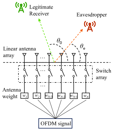
Figure 1: Illustration of the TMA OFDM-enabled DM transmitter.

Before being radiated into the half space, $\theta\in[0,\pi]$, the OFDM symbol needs to be multiplied by antenna weights $\{w_{n}\}_{n=1,2,...,N}$ and manipulated by a ON-OFF temporal function $U(t)$ that controls the switch array periodically. Let the wavelength $\lambda_{0}$ associate with $f_{0}$. The signal transmitted by the TMA OFDM system can be expressed as

$${y}(t,\theta)=\frac{1}{\sqrt{N}}\sum\limits_{n=1}^{N}{x}(t)w_{n}U_{n}(t)e^{j(n-1)\pi\cos\theta}.$$ (2)

In order to focus the beam towards the direction of the legitimate user, $\theta_{0}$, we set $w_{n}=e^{-j(n-1)\pi\cos\theta_{\rm 0}}$. The ON-OFF switching function $U_{n}(t)$ is designed as a periodic square waveform with the time period being $T_{s}$. On denoting the normalized switch ON time instant and the normalized ON time duration as $\tau_{n}^{o}$ and $\Delta\tau_{n}$, respectively, we can express $U_{n}(t)$ as Fourier series as follows:

$$U_{n}(t)=\sum_{-\infty}^{\infty}a_{mn}e^{j2m\pi f_{s}t},$$ (3)

where

$$a_{mn}=\Delta\tau_{n}\operatorname{sinc}(m\pi\Delta\tau_{n})e^{-jm\pi(2\tau_{n}^{o}+\Delta\tau_{n})}.$$ (4)

Here $\operatorname{sinc}(\cdot)$ is an unnormalized sinc function. By combining the above equations, we write the transmitted symbol as

$${y}(t,\theta)=\frac{1}{\sqrt{NK}}\sum_{l=1}^{K}s_{k}e^{j2\pi[f_{0}+(l-1)f_{s}]t}\sum_{m=-\infty}^{\infty}e^{j2m\pi f_{s}t}V_{m},$$ (5)

where

$$V_{m}=\sum\limits_{n=1}^{N}a_{mn}e^{j(n-1)\pi(\cos\theta-\cos\theta_{\rm 0})}.$$ (6)

Then, the signal seen in direction $\theta$ on the $i$-th subcarrier equals

$${y}_{i}(t,\theta)=\frac{1}{\sqrt{NK}}\sum\limits_{l=1}^{K}s_{k}e^{j2\pi[f_{0}+(l-1)f_{s}]t}V_{i-l}.$$ (7)

After OFDM demodulation, the received data symbol on the $i$-th subcarrier can be expressed as $y_{i}(\theta)=1/\sqrt{NK}\sum_{l=1}^{K}s_{k}V_{i-l}$. The received signals on all subcarriers without noises, put in vector $\boldsymbol{y}$, can be expressed as

$$\boldsymbol{y}=\boldsymbol{V}\boldsymbol{s},$$ (8)

where $\boldsymbol{V}\in\mathbb{C}^{K\times K}$ is a Toeplitz matrix defined as

$$\boldsymbol{V}=\frac{1}{\sqrt{NK}}\left[\begin{array}[]{ccccc}V_{0}&V_{-1}&\cdots&V_{-(K-2)}&V_{-(K-1)}\\ V_{1}&V_{0}&\cdots&V_{-(K-3)}&V_{-(K-2)}\\ \vdots&\vdots&\ddots&\vdots&\vdots\\ V_{K-2}&V_{K-3}&\cdots&V_{0}&V_{-1}\\ V_{K-1}&V_{K-2}&\cdots&V_{1}&V_{0}\end{array}\right],$$ (9)

and $\boldsymbol{s}=[s_{1},s_{2},\cdots,s_{K}]^{T}$. In order to implement DM functionality, $\tau_{n}^{o}$ and $\Delta\tau_{n}$ must be chosen to satisfy $V_{m\neq 0}(\tau_{n}^{o},\Delta\tau_{n},\theta=\theta_{0})=0$ and $V_{m=0}(\tau_{n}^{o},\Delta\tau_{n},\theta=\theta_{0})\neq 0$. These can be achieved by the following three conditions [27]:

• (C1) $\Delta\tau_{n},\tau_{n}^{o}\in\{\frac{h-1}{N}\}_{h=1,2,...,N}$ (note that the subscript $n$ is not necessarily equal to $h$);

• (C2) $\tau_{p}^{o}\neq\tau_{q}^{o},\Delta\tau_{p}=\Delta\tau_{q}=\Delta\tau$ for $p\neq q$;

• (C3) $\sum_{n=1}^{N}\Delta\tau_{n}\neq 0$.

By substituting these three conditions into the above equations, we can find that along $\theta_{0}$, $\boldsymbol{V}$ is a diagonal matrix and the received OFDM signal equals ${y}(t,\theta_{0})=\Delta\tau\sqrt{N/K}{s}(t)$. In all other directions, the signal of each subcarrier contains the harmonic signals from all other subcarriers, which gives rise to the so-called scrambling, hence achieving the PLS. Taking into account the additive noise $\boldsymbol{z}=[z_{1},\cdots,z_{k},\cdots,z_{K}]^{T}$, where $z_{k}$ is a i.i.d. Gaussian random variable with zero mean and the same variance, the received signals can be written as

$$\boldsymbol{y}=\boldsymbol{V}\boldsymbol{s}+\boldsymbol{z}.$$ (10)

In the following, we will consider the centered and whitened received signal, i.e.,

$$\tilde{\boldsymbol{y}}=\boldsymbol{A}\boldsymbol{y}=\tilde{\boldsymbol{V}}\boldsymbol{s}+\boldsymbol{A}\boldsymbol{z}$$ (11)

where $\boldsymbol{A}$ is the whitening matrix, obtained based on the eigenvector matrix of the covariance of $\mathbf{y}$ [37]. For independent, zero-mean and unit-variance inputs, $s_{k}$, and noiseless case, we have

$$E\{\tilde{\boldsymbol{y}}\tilde{\boldsymbol{y}}^{{\dagger}}\}=\tilde{\boldsymbol{V}}E\{\boldsymbol{s}\boldsymbol{s}^{{\dagger}}\}\tilde{\boldsymbol{V}}^{{\dagger}}=\tilde{\boldsymbol{V}}\tilde{\boldsymbol{V}}^{{\dagger}}=\boldsymbol{I}.$$ (12)

III On Defying the TMA scrambling by the Eavesdropper

Let us assume the presence of an eavesdropper in direction $\theta_{e}$ ($\theta_{e}\neq\theta_{0}$). Due to (C1)-(C3), one can see that, along direction $\theta_{e}$, the received OFDM signal on each subcarrier is scrambled by the data symbols modulated onto all other subcarriers, since for $\theta=\theta_{e}$, $\boldsymbol{V}$ is not diagonal.

Note that $\boldsymbol{y}$ in (11), contains linear mixtures of the elements of $\boldsymbol{s}$. Both $\boldsymbol{s}$, $\tilde{\boldsymbol{V}}$ are unknown to the eavesdropper, so the recovery of $\boldsymbol{s}$ can be viewed as a blind source separation problem. In communications, the elements of $\boldsymbol{s}$ are typically statistically independent with each other and non-Gaussian. Thus, the eavesdropper can leverage an ICA method to estimate $\tilde{\boldsymbol{V}}$, and then, recover $\boldsymbol{V}$ based on $\boldsymbol{A}$.

In this section, we first introduce the application of ICA, based on which we propose CMICA, an algorithm for estimating the mixing matrix using short-length data, and then we show how to resolve the ambiguities and fully recover the source signals.

III-A The Proposed CMICA for Estimating the Mixing Matrix

The ICA attempts to recover the mixed data based on the fact that the sum of two or more independent, non-Gaussian random variables is more Gaussian than the original variables. Hence, the goal of ICA is to find an unmixing matrix $\boldsymbol{W}=[\boldsymbol{w}_{1},\cdots,\boldsymbol{w}_{l},\cdots,\boldsymbol{w}_{K}]^{T}$ that maximizes the non-Gaussianity of $\boldsymbol{W}\tilde{\boldsymbol{y}}$. When $v=\boldsymbol{w}_{l}^{T}\tilde{\boldsymbol{y}}$ is least Gaussian it is actually corresponding to one element of $\boldsymbol{s}$ [37]. To find more elements of $\boldsymbol{s}$ we need to constrain the search to the space that gives estimates uncorrelated with the previous ones.

The non-Gaussianity can be quantified via the kurtosis or the negentropy, which can be both formulated as

$$J_{G}(\boldsymbol{w})=E\{G(|\boldsymbol{w}^{{{\dagger}}}\tilde{\boldsymbol{y}}|^{2})\},$$ (13)

where $G$ is a smooth contrast function, chosen as $G(v)=\frac{1}{2}v^{2}$ to approximate kurtosis, and $G(v)=-\exp(-v/2)$ to approximate negentropy. Since $\tilde{\boldsymbol{y}}$ is white and zero-mean, $v$ has zero mean and has unit variance.

Here, we need to maximize the sum of $K$ non-Gaussianity quantifiers, one for each subcarrier. We obtain the following constrained optimization problem:

$$\max \sum_{l=1}^{K}J_{G}(\boldsymbol{w}_{l})$$ (14)

s.t. $$\boldsymbol{w}_{i}^{{\dagger}}\boldsymbol{w}_{j}=\zeta_{ij},$$

where $\zeta_{ij}=1$ for $i=j$ and $\zeta_{ij}=0$ otherwise. To solve the problem of (14), we can adopt a FastICA algorithm [41], by which the unmixing weights are updated using a fixed-point iteration scheme. This iteration scheme involves estimating the new weight vector, normalizing it, and then ensuring that it is decorrelated from the previously estimated ones.

III-A1 Considering constant modulus signals to reduce the required samples

Even though FastICA converges fast, it needs a large sample set to achieve low estimation error. This is because the non-Gaussianity metric is computed based on the mean of a function of the collected samples, and more samples lead to better mean estimate and better ICA estimates. Good ICA estimates are essential for the subsequent steps of resolving the ambiguities. However, obtaining a large sample of data may not be possible in dynamic communication environments, or in case in which the TMA system parameters vary in time. Next, we will show how one can obtain good estimates with a small number of data samples.

Let us assume that the source symbols are constant-modulus, for example $M$-PSK, which are very common in communication systems. On omitting noise and denoting the optimal $\boldsymbol{w}_{i}$ by $\boldsymbol{w}_{i}^{opt}$, we have that

$$|(\boldsymbol{w}_{i}^{opt})^{{\dagger}}\tilde{\boldsymbol{y}}|=|s_{j}|,s_{j}\in\boldsymbol{s},$$ (15)

Let us for simplicity omit the subscript ‘$i$’. On denoting by $D_{L}$ and $D_{S}$, a large-sample and a small-sample dataset, respectively, we can obtain a sample estimate of the non-Gaussianity metric, denoted as $\hat{J}_{G}$, under $D_{L}$ as

$$\hat{J}_{G}(\boldsymbol{w})|_{\tilde{\boldsymbol{y}}\in D_{L}}=\frac{1}{n_{L}}\sum_{\tilde{\boldsymbol{y}}\in D_{L}}G(|\boldsymbol{w}^{{{\dagger}}}\tilde{\boldsymbol{y}}|^{2}),$$ (16)

and under $D_{S}$ as

$$\hat{J}_{G}(\boldsymbol{w})|_{\tilde{\boldsymbol{y}}\in D_{S}}=\frac{1}{n_{S}}\sum_{\tilde{\boldsymbol{y}}\in D_{S}}G(|\boldsymbol{w}^{{{\dagger}}}\tilde{\boldsymbol{y}}|^{2}),$$ (17)

where ${n_{L}}$ and ${n_{S}}$ are the number of samples in $D_{L}$ and $D_{S}$, respectively. Incorporating (15) into (16) and (17), we can get

$$\hat{J}_{G}(\boldsymbol{w}^{opt})|_{\tilde{\boldsymbol{y}}\in D_{L}}=\hat{J}_{G}(\boldsymbol{w}^{opt})|_{\tilde{\boldsymbol{y}}\in D_{S}}=G(|s|^{2}).$$ (18)

Let us denote by $\boldsymbol{w}_{D_{L}}^{opt}$ and $\boldsymbol{w}_{D_{S}}^{opt}$ the estimate of the optimal solution of (14) using $D_{L}$ and $D_{S}$, respectively. Although based on the invariance of $\hat{J}_{G}(\boldsymbol{w}^{opt})$ to the data length, which is shown in (18), we cannot make any claims about the behavior of $\hat{J}_{G}(\boldsymbol{w})$ as the data length changes, we observe in simulations that $\hat{J}_{G}(\boldsymbol{w})$ does not change abruptly with the sample length and further, $\boldsymbol{w}_{D_{S}}^{opt}$ is close to $\boldsymbol{w}_{D_{L}}^{opt}$. Based on the above observation, we can find $\boldsymbol{w}^{opt}$ by solving for $\boldsymbol{w}_{D_{S}}^{opt}$.

III-A2 Solving for $\boldsymbol{w}_{D_{S}}^{opt}$ in CMICA

We propose a two-stage method to obtain $\boldsymbol{w}_{D_{S}}^{opt}$ based on $D_{s}$. In the first stage, the Newton iteration and the decorrelation operation are applied to solve the problem of (14), along the lines of FastICA [40]. The main difference between the second stage and the first stage is that the decorrelation operation is dropped.

Let us first consider a noiseless case, i.e., $\tilde{\boldsymbol{y}}=\tilde{\boldsymbol{V}}\boldsymbol{s}$. The Lagrangian of the problem of (14) is

$$L(\boldsymbol{w},\lambda)=E\{G(|\boldsymbol{w}^{{{\dagger}}}\tilde{\boldsymbol{y}}|^{2})\}-\lambda(\|\boldsymbol{w}\|^{2}-1),$$ (19)

where $\lambda$ is the Lagrangian multiplier. Adopting an approximate Newton iteration method [40], we obtain an initial estimation of $\boldsymbol{w}_{D_{S}}^{opt}$ via the following iteration:

$$\boldsymbol{w}:=\boldsymbol{w}-\frac{E\{\tilde{\boldsymbol{y}}(\boldsymbol{w}^{{\dagger}}\tilde{\boldsymbol{y}})^{*}g(|\boldsymbol{w}^{{\dagger}}\tilde{\boldsymbol{y}}|^{2})\}-\lambda\boldsymbol{w}}{E\{g(|\boldsymbol{w}^{{\dagger}}\tilde{\boldsymbol{y}}|^{2})+2|\boldsymbol{w}^{{\dagger}}\tilde{\boldsymbol{y}}|^{2}g^{\prime}(|\boldsymbol{w}^{{\dagger}}\tilde{\boldsymbol{y}}|^{2})\}-\lambda},$$ (20)

where we use MATLAB notation for the iterative update of $\boldsymbol{w}$, and $\lambda=E\{|\boldsymbol{w}^{{\dagger}}\tilde{\boldsymbol{y}}|g(|\boldsymbol{w}^{{\dagger}}\tilde{\boldsymbol{y}}|^{2})\}$, with $g$ and $g^{\prime}$ being the first-order and the second-order derivative of $G$, respectively. Subsequently, the mixing matrix $\boldsymbol{W}$ constructed based on $\boldsymbol{\boldsymbol{w}}$ is decorrelated as follows:

$$\boldsymbol{W}:=\boldsymbol{W}(\boldsymbol{W}^{{\dagger}}\boldsymbol{W})^{-1/2}.$$ (21)

After the Newton iteration converges, the obtained $\boldsymbol{w}$ is only a coarse estimate of $\boldsymbol{w^{opt}}$, while the resulting $\boldsymbol{s}$ is not white, i.e., ${\rm cov}(\boldsymbol{s},\boldsymbol{s})\neq\boldsymbol{I}$, and hence $\tilde{\boldsymbol{V}}\tilde{\boldsymbol{V}}^{{\dagger}}\neq\boldsymbol{I}$ due to the used sample size is not large enough. There is no point trying to use decorrelation further. Beyond that point, we introduce a fine-tuning stage to refine this coarse estimate. We can do this with the gradient descent method, where by adjusting the step size we have better control of the fine-tuning as compared to the Newton method. Using the gradient descent method to maximize (19) we get the update

$$\boldsymbol{w}:=\boldsymbol{w}+\mu(E\{\tilde{\boldsymbol{y}}(\boldsymbol{w}^{{\dagger}}\tilde{\boldsymbol{y}})^{*}g(|\boldsymbol{w}^{{\dagger}}\tilde{\boldsymbol{y}}|^{2})\}-\lambda\boldsymbol{w}),$$ (22)

where $\mu$ is the step size. In this stage we skip the decorrelation operation, and only normalize $\boldsymbol{w}$ after each iteration to satisfy the constraint $\|\boldsymbol{w}\|^{2}=1$. After fine-tuning, we obtain $\boldsymbol{W}_{D_{S}}^{opt}$.

In the noisy case, i.e., $\tilde{\boldsymbol{y}}=\tilde{\boldsymbol{V}}\boldsymbol{s}+\boldsymbol{Az}$, the contribution of the colored Gaussian noise, $\boldsymbol{Az}$, is suppressed when using kurtosis as the non-Gaussianity metric. When using negentropy as the non-Gaussianity metric, the Gaussian moments-based method [42] can be applied to estimate the mixing matrix from colored noisy data. We summarize the above two-stage CMICA algorithm in Algorithm 1.

Algorithm 1 Proposed CMICA Algorithm

1:Preprocess the collected data $\boldsymbol{y}$ and initialize $\boldsymbol{W}$ randomly;

2:Start the first stage:

3:for each $i=1,2,...,K$ do

4:     Update $\boldsymbol{w}_{i}$ according to (20);

5:end for

6:Decorrelate $\boldsymbol{W}$ according to (21);

7:Repeat step 3 $\sim$ 6 until convergence or maximal iteration number;

8:Start the second stage:

9:for each $i=1,2,...,K$ do

10:     Update $\boldsymbol{w}_{i}$ according to (22);

11:     Normalize $\boldsymbol{w}_{i}$ by $\boldsymbol{w}_{i}=\boldsymbol{w}_{i}/\|\boldsymbol{w}_{i}\|$;

12:end for

13:Repeat step 9 $\sim$ 12 until convergence or maximal iteration number.

III-B Proposed KNN-Based Scheme for Resolving Ambiguities

After obtaining $\boldsymbol{W}$, $(\boldsymbol{WA})^{-1}$ is most probably not equal to the actual mixing matrix $\boldsymbol{V}$ since there exist scaling and permutation ambiguities in $\boldsymbol{W}$ [37], which would prevent the correct recovery of source symbols. To resolve these ambiguities, we need to exploit prior knowledge about the TMA OFDM system. Assume that the eavesdropper knows (i) the OFDM specifics of the transmitted signals, like the number of subcarriers, $K$, (ii) the data modulation scheme, (iii) the Toeplitz structure of $\boldsymbol{V}$ and (iv) the rules (C1)-(C3) for implementing TMA. The rules (C1)-(C3) define a set of values for TMA parameters, therefore, knowledge of the rules does not imply any knowledge of the specific parameters used by the TMA.

III-B1 Resolving the amplitude scaling ambiguity

First, the scaling ambiguity arises because $\boldsymbol{y}=\boldsymbol{V}\boldsymbol{s}$ can be written as $\boldsymbol{y}=\sum_{i}(\alpha_{i}\boldsymbol{V}(:,i))(s_{i}/\alpha_{i})$ for an arbitrary $\alpha_{i}$. The ICA algorithm cannot distinguish between $s_{i}$ and $s_{i}/\alpha_{i}$ since both of them have the same level of non-Gaussianity. Let us separate the scaling ambiguity into amplitude and phase ambiguity. By knowing the transmit constellation, the eavesdropper knows the amplitudes of the source signals. As a result, the eavesdropper knows how much the amplitude of the recovered signals is scaled, and can thus recover the amplitude scaling ambiguity. Before resolving the phase ambiguity, the eavesdropper will need to reorder the estimated mixing matrix correctly, which is discussed in the next subsection.

III-B2 Resolving the permutation ambiguity

The permutation ambiguity arises because $\boldsymbol{y}$ will not change if the elements of $\boldsymbol{s}$ are permuted and the columns of $\boldsymbol{V}$ are accordingly permuted. Therefore, ICA cannot identify the recovered data symbols in the right order, i.e., it cannot match each demixed data symbol with the right subcarrier. To solve this issue, we proceed as follows. We define $\boldsymbol{F}\buildrel\triangle\over{=}(\boldsymbol{WA})^{-1}$. In the absence of ambiguities, $\boldsymbol{F}$ would be equal to $\boldsymbol{V}$ forming a Toeplitz matrix. However, due to the presence of ambiguities, this is not the case. We propose reordering $\boldsymbol{F}$ by assessing how closely the reordered $\boldsymbol{F}$ approximates a Toeplitz matrix structure. Exhaustive reordering is impractical due to the $K!$ possible orderings, resulting in prohibitive computational cost. The reordering process to be explained next has complexity $O(K^{3})$.

Based on (9), there are $K$ identical elements in the main diagonal of $\boldsymbol{V}$, and $K-1$, $K-2$, …, $1$ identical elements in other diagonals above or under the main diagonal. Since the values of $V_{-(K-1)},\cdots,V_{0},\cdots,V_{K-1}$ are different according to (6), the main diagonal can solely determine the Toeplitz structure of $\boldsymbol{V}$. Therefore, when $\boldsymbol{F}$ is reordered correctly, its main diagonal elements will be nearly identical. We should note that due to estimation errors within ICA, the estimated diagonal elements will not be exactly the same. So we propose to focus only on the main diagonal elements to reorder $\boldsymbol{F}$ and achieve low computational complexity. Specifically, we first calculate the amplitude of each element in $\boldsymbol{F}$ and get a new matrix $\boldsymbol{Q}$, the $i$th column of which is denoted by $\boldsymbol{q}_{i}$. Then we select the first $k$ elements of $\boldsymbol{q}_{i}$, i.e., $\boldsymbol{q}_{i}(1:k)$, as the reference vector, and put $\boldsymbol{q}_{i}$ in the first column of an empty matrix $\bar{\boldsymbol{F}}$, which is used to store the reordered $\boldsymbol{F}$. Next, we compare $\boldsymbol{q}_{j\neq i}(2:k+1)$ with the selected reference vector based on the cosine similarity and put the least similar vector in the second column of $\bar{\boldsymbol{F}}$. In turn, we obtain $K-k+1$ reordered columns in $\bar{\boldsymbol{F}}$. For the remaining unsorted $k-1$ columns in $\boldsymbol{Q}$, we take the average of the main diagonal elements of the matrix formed by those $K-k+1$ reordered columns as the reference, and put these unsorted $k-1$ columns in the corresponding placements according to the fact that the main diagonal elements of the mixing matrix should be the same. For each of the $K$ reference vectors, $\boldsymbol{q}_{i}(1:k),i=1,\cdots,K$, we obtain a matrix $\bar{\boldsymbol{F}}$. Out of them, we select the $k$ matrices with the least normalized standard deviation of their main diagonal elements, and let the phase ambiguity resolving approach, to be described next, find the most plausible ${\boldsymbol{F}}$.

III-B3 Resolving phase scaling ambiguity

At this step, $\boldsymbol{F}$ and $\boldsymbol{s}$ denote the results of the above described processes that resolved the amplitude scaling amplitude and permutation ambiguities. The phase ambiguity is introduced when $\alpha_{i}$ is strictly complex. Let us consider $M$-PSK modulated source symbols. Each source signal can have up to $M$ phase transformations, hence there are $M$ possible phases for each column of $\boldsymbol{F}$, and in total $M^{K}$ phase possibilities for $\boldsymbol{F}$. The Toeplitz constraint can reduce the $M^{K}$ possibilities to $M$; this is because the phases of the diagonal elements of $\boldsymbol{F}$ must be the same. We define these $M$ possibilities for $\boldsymbol{F}$ as $\boldsymbol{F}_{1},\boldsymbol{F}_{2},...,\boldsymbol{F}_{M}$. The core principle of resolving the phase ambiguity is to check if there exist a set of TMA parameters, i.e, $N,\Delta\tau,\{\tau_{n}^{o}\}_{n=1,2,...,N},\theta_{e},\theta_{0}$, that correspond to a unique matrix in the set $\{\boldsymbol{F}_{u},{u=1,2,...,M}\}$. If such unique matrix does not exist then the phase uncertainty cannot be eliminated. The feasible TMA parameters must satisfy the rules defined in (C1)-(C3) in Section II and $N\in\mathbb{N}^{+}$, $\theta_{e},\theta_{0}\in(0,\pi)$. To this end, we proceed as follows. From (4) and (6) we have

$$V_{m}=0,m=\pm N,\pm 2N,\pm 3N,\cdots$$ (23)

This is because the $\operatorname{sinc}$ term will be 0 when $m=\pm N,\pm 2N,\pm 3N,\cdots$ We can utilize (23) to find the value of $N$ from $\boldsymbol{F}$. Then, let $\phi=\cos\theta_{e}-\cos\theta_{0}$. From (6) we obtain

$$\begin{split}V_{0}&=\Delta\tau\sum\limits_{n=1}^{N}e^{j(n-1)\pi\phi}=\Delta\tau\frac{1-e^{jN\pi\phi}}{1-e^{j\pi\phi}}\\ &=\Delta\tau\frac{\sin(\frac{N}{2}\pi\phi)}{\sin(\frac{1}{2}\pi\phi)}e^{j\frac{(N-1)}{2}\pi\phi},\end{split}$$ (24)

where $\phi\neq\pm 2/N,\pm 4/N,\pm 6/N,\cdots$ On assuming that $\phi$ is known, which can be obtained via direction finding techniques by the eavesdropper, we will know the actual phase of $V_{0}$ from (24), denoted as $\angle V_{0}$, since it is determined only by $N$ and $\phi$. Next, for each possible $\boldsymbol{F}_{u}$ we check whether the following holds:

$$\angle V_{0}=\angle\boldsymbol{F}_{u}(1,1),$$ (25)

where $\boldsymbol{F}_{u}(1,1)$ is the main diagonal element of $\boldsymbol{F}_{u}$. Meanwhile, we need to check whether there exists $\Delta\tau$ constrained by the rules (C1)-(C3) that satisfies

$$\begin{split}&|V_{0}|=|\boldsymbol{F}_{u}(1,1)|.\end{split}$$ (26)

By (23), (25) and (26), we can find the solutions of $N,\Delta\tau,\phi$ for only one of $\{\boldsymbol{F}_{u},{u=1,2,...,M}\}$ since there is a fixed phase difference, i.e., $\frac{2\pi}{M}$, between $\boldsymbol{F}_{u}(1,1)$ and $\boldsymbol{F}_{u+1}(1,1)$. Therefore, the phase ambiguity is resolved when $\phi$ is known.

Algorithm 2 KNN-based Ambiguity Resolving Algorithm

1:Set $S=\{1,2,...,K\}$;

2:for each $i=1,2,...,K$ do

3:     Take $\boldsymbol{q}_{i}(1:k)$ as the reference vector and put $\boldsymbol{q}_{i}$ in the first column of $\bar{\boldsymbol{F}}$;

4:     Remove $i$ from $S$;

5:     for each $d=2,3,...,K-k+1$ do

6:         Find $\boldsymbol{q}_{j}(d:d+k-1)$, $j\in S$ that is the closest to $\boldsymbol{q}_{i}(1:k)$ based on the cosine similarity;

7:         Put $\boldsymbol{q}_{j}$ in the $d$-th column of $\bar{\boldsymbol{F}}$;

8:         Remove $j$ from $S$;

9:     end for

10:     Form a matrix $\boldsymbol{B}_{i}$ by the above $K-k+1$ reordered columns and take the average of main diagonal of $\boldsymbol{B}_{i}$ as $b_{i}$;

11:     Find the remaining $k-1$ unsorted columns based on $b_{i}$;

12:     Obtain a reordered $\bar{\boldsymbol{F}}_{i}$ and then take the normalized standard deviation of its main diagonal as $\sigma_{i}$

13:end for

14:Let $\boldsymbol{\sigma}=[\sigma_{1},...,\sigma_{K}]$ and select the first $k$ smallest elements in $\boldsymbol{\sigma}$, by which we obtain $k$ reordered $\bar{\boldsymbol{F}}$ and accordingly $k$ reordered $\boldsymbol{F}$;

15:for each reordered $\boldsymbol{F}$ do

16:     Obtain $\{\boldsymbol{F}_{u},u=1,...,M\}$ according to the transmission constellation and the Toeplitz constraint;

17:     for each $\boldsymbol{F}_{u}$ do

18:         Estimate $N$ according to (23);

19:         if $\phi$ is known then

20:              Check if there are solutions to (25) and (26);

21:         else

22:              Check if there are solutions to (27) and (25), (26), (28);

23:         end if

24:     end for

25:end for

When $\phi$ is not known, we can proceed as follows. The ratio of the real part and imaginary part of $V_{0}$, denoted as $\gamma$, is

$$\gamma=\frac{1}{\tan{\frac{N-1}{2}\pi\phi}}.$$ (27)

After estimating $N$ from (23), we can estimate all possible values of $\phi$, $\phi\in(-2,2)$ from (27) for each $\{\boldsymbol{F}_{u},u=1,...,M\}$. Then, for each found $\phi$, we check if there are solutions to the equation (25) and (26). After that, we can find the feasible values of $N,\Delta\tau$ and $\phi$ for at least one of $\{\boldsymbol{F}_{u},u=1,...,M\}$; if two or more $\boldsymbol{F}$ are found, we further check whether there exists $\{\tau_{n}^{o}\}_{n=1,2,...,N}$ that satisfies

$$\boldsymbol{V}(\tau_{n}^{o},\Delta\tau,N,\phi)=\boldsymbol{F},$$ (28)

where $\{\tau_{n}^{o}\}_{n=1,2,...,N}$ are subject to (C1)-(C3), and $N,\Delta\tau$ and $\phi$ are the found values by solving (23), (25) and (26). Since there are constraints on the feasible TMA parameters as stated above, it is possible to find only one $\boldsymbol{F}$ among $\{\boldsymbol{F}_{u},u=1,...,M\}$ by solving the equation (23), (25), (26), (27) and (28). This means that the eavesdropper could still eliminate the phase uncertain even when $\phi$ is not known. We summarize the complete ambiguity resolving process in Algorithm 2.

IV Defending the TMA scrambling

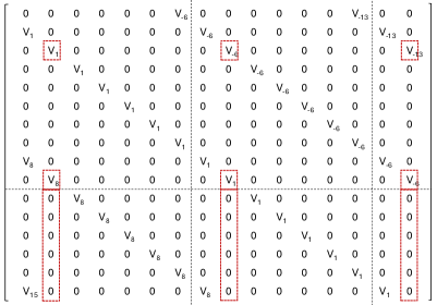
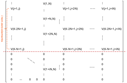
Figure 2: Illustration of $\boldsymbol{V}$ when $\phi=\pm 2/N,\pm 4/N,\pm 6/N,\cdots$ and $\tau_{n}^{o}=(n-1)/N$: (a) an specific example with $K=16$, $N=7$; (b) a general diagram used for proving Lemma 1.

IV-A Conditions for A Secure TMA

There are two scenarios where the TMA OFDM system is sufficiently secure: when $\boldsymbol{V}$ is rank-deficient and when there is non-uniqueness in the ON-OFF switching pattern. In the former case, there are multiple solutions for $\boldsymbol{s}$ when solving the problem of $\boldsymbol{y}=\boldsymbol{V}\boldsymbol{s}$. The non-uniqueness means that there are multiple ON-OFF switching patterns, i.e., multiple groups of $\Delta\tau$ and $\{\tau_{n}^{o}\}_{n=1,2,...,N}$ when trying to defy the scrambling.

When $\phi=\cos\theta_{e}-\cos\theta_{\rm 0}=\pm 2/N,\pm 4/N,\pm 6/N,\cdots$, the aforementioned two cases become feasible. Specifically, on using $\phi=\pm 2/N,\pm 4/N,\pm 6/N,\cdots$ and $\tau_{n}^{o}=(n-1)/N$ in (6), we get

$$V_{m}\begin{dcases}\neq 0&m=1+iN,\,i=0,\pm 1,\pm 2,\cdots\\ =0&\text{otherwise}\end{dcases}$$ (29)

Based on the above observations, we obtain the following corollary.

Corollary 1.

The interval of the nearest two non-zero elements in the same row or column of $\boldsymbol{V}$ is $N$.

We show an example of this special mixing matrix for $N=7,K=16$ in Fig. 2(a). For this kind of mixing matrix, we can prove the following lemma

Lemma 1.

$\boldsymbol{V}$, as defined in (9), is not full-rank when $iN\neq K,\forall i\in\mathbb{N^{+}}$.

Proof.

Suppose $iN\neq K,\forall i\in\mathbb{N^{+}}$. Let us set $K=iN+j$, where $j$ is the reminder, $1\leq j\leq N-1$. Let us divide the matrix $\boldsymbol{V}$ into two parts: $\boldsymbol{V}^{+}\in\mathbb{C}^{K-N+1\times K}$ and $\boldsymbol{V}^{-}\in\mathbb{C}^{N-1\times K}$, as shown in Fig. 2 (b); the parts are separated by the red dotted line in Fig. 2 (b). According to Corollary 1, the $N$-th column of $\boldsymbol{V}$ has $i+1$ non-zero elements. Also, its $(i+1)$-th non-zero element is $\boldsymbol{V}(1+iN,N)$, and is located in $\boldsymbol{V}^{-}$ since $K-N+2\leq 1+iN\leq K$.

Along the diagonal including $\boldsymbol{V}(1+iN,N)$, we can find one non-zero element $\boldsymbol{V}(K-N+1,j)$. This is because, the elements onto the diagonal including $\boldsymbol{V}(1+iN,N)$ are all the same and hence non-zero according to the Toeplitz constraint. For the non-zero element located in the $K-N+1$-th row, its index of column is $N-((1+iN)-(K-N+1))=K-iN=j$. So we get the non-zero element $\boldsymbol{V}(K-N+1,j)$.

For the $j$-th column of $\boldsymbol{V}$, we know that its $N-1$ elements located in $\boldsymbol{V}^{-}$ are all 0, as shown in Fig. 2 (b), according to Corollary 1. For its part located in $\boldsymbol{V}^{+}$, there are $i$ non-zero elements since $K-N+1=(i-1)N+j+1$ and it has the non-zero elements $\boldsymbol{V}(j+1,j)$, $\boldsymbol{V}(N+j+1,j)$, $\cdots$, $\boldsymbol{V}((i-1)N+j+1,j)$. We have similar results for the $(j+N)$-th, $(j+2N)$-th, $\cdots$, $(j+iN)$-th (exactly the $K$-th) column. Therefore, we have $i+1$ columns in $\boldsymbol{V}$ that have only $i$ non-zero elements located in the $(j+1)$-th, $(N+j+1)$-th, $\cdots$, $((i-1)N+j+1)$-th rows of $\boldsymbol{V}^{+}$ and the elements located in $\boldsymbol{V}^{-}$ are all 0.

According to the Leibniz formula for finding the determinant of a matrix [43], after selecting $i$ non-zero elements located in different rows out of the corresponding $i+1$ columns, there must be one column left. For the column left, its row indices of non-zero elements have been occupied, so there must be 0 existing in the Leibniz formula. Therefore, the determinant of $\boldsymbol{V}$ is zero and Lemma 1 is proved. ∎

As shown in Fig. 2 (a), $K=16$ and $N=7$, so there is no $i\in\mathbb{N^{+}}$ that satisfies $K=iN$. From this figure, we can see there exist three columns that have only two non-zero elements located in $\boldsymbol{V}^{+}$, which are marked by the red boxes.

When $\phi=\pm 2/N,\pm 4/N,\pm 6/N,\cdots$ and $\tau_{n}^{o}\neq(n-1)/N$, there exist possibly multiple groups of $\Delta\tau$, $\{\tau_{n}^{o}\}_{n=1,2,...,N}$ and $\boldsymbol{s}$ that correspond to the same $\boldsymbol{y}$. In fact, it is intractable to solve for multiple group of $\Delta\tau$, $\{\tau_{n}^{o}\}_{n=1,2,...,N}$ and $\boldsymbol{s}$ directly from $\boldsymbol{y}=\boldsymbol{V}\boldsymbol{s}$ after incorporating $\phi=\pm 2/N,\pm 4/N,\pm 6/N,\cdots$ into it, since $\boldsymbol{V}$ contains many $\sin$ and $\exp$ terms and it is a transcendental equation. To shed light on the reason, taking $\phi=2/N,N=K=4$ and BPSK modulation symbol [-1, +1], we can obtain two different groups of $\Delta\tau$, $\{\tau_{n}^{o}\}_{n=1,2,...,N}$ and $\boldsymbol{s}$, i.e., $1/N$, $\{3/N,1/N,2/N,0\}$, $[+1,-1,-1,+1]$ and $3/N$, $\{0,2/N,3/N,1/N\}$, $[-1,+1,+1,-1]$ that both correspond to the same $\boldsymbol{y}$. By checking further this example, we find it is the periodicity and parity of the $\sin$ and $\exp$ terms (the $\exp$ term can be converted to $\sin$ and $\cos$) in $\boldsymbol{V}$ that lead to the non-uniqueness of ON-OFF switching pattern.

IV-B Measures for Defending the Scrambling

We can enhance the wireless security of the TMA transmitter by rotating it at a certain angle $\theta_{r}$ to satisfy $\cos(\theta_{e}+\theta_{r})-\cos(\theta_{0}+\theta_{r})=\pm 2/N,\pm 4/N,\pm 6/N,\cdots$. In this case we need to know the eavesdropper location. Based on the aforementioned conditions for a secure TMA, it is impossible for an eavesdropper to apply our proposed defying scheme to resolve the ambiguity when $\phi=\pm 2/N,\pm 4/N,\pm 6/N,\cdots$. Furthermore, the eavesdropper cannot crack the TMA OFDM system completely by any means under the first class of condition, as the system is underdetermined, thereby ensuring sufficient security.

We can also design some mechanisms to defend the TMA scrambling against the eavesdroppers by virtue of the weakness of ICA. Since the above ICA can work only in stationary environments and necessitates data for estimating the required higher-order statistics, we can disturb the applicability of ICA by changing the mixing matrix of TMA over time. This can be done by selecting randomly $\{\tau_{n}^{o}\}_{n=1,2,...,N}$ in each OFDM symbol period according to $\tau_{n}^{o}\in\{\frac{h-1}{N}\}_{h=1,2,...,N}$ and $\tau_{p}^{o}\neq\tau_{q}^{o}$. Meanwhile this mechanism is able to maintain the DM functionality as it still satisfies the scrambling scheme. The cost is that this will increase the hardware design complexity since it requires the switch ON-OFF pattern changing frequently. Moreover, we can degrade ICA by disturbing the independence of source signals, which can be achieved by randomly assigning some identical symbols to be transmitted on multiple subcarriers but it will result in lower bit rate. These two methods do not require knowledge of the eavesdropper location.

V NUMERICAL RESULTS

In this section, we present numerical results to evaluate our proposed TMA scrambling defying and defending schemes. First of all, we summarize the main parameters and their definitions used in the simulations in Table I in order to enhance the readability of the paper. Then, we simulate a TMA OFDM-enabled DM system with $N=7$ antennas as the same as in [27]. We set the TMA parameters according to the rules (C1)-(C3) and adopt the BPSK modulation. Also, We assume perfect channel knowledge in the system and use BER as the performance metric to evaluate the proposed approaches. For the non-white noise due to the whitening, we adopt the negentropy as the non-Gaussianity metric and the Gaussian moments-based method proposed in [42] to tackle with it. The value of $\phi$ is assumed to be known by the eavesdropper and $k=3$ unless otherwise specified. For other parameters, they are specified in the corresponding experiments. The results and analyses are as follows.

TABLE I: Main Notations and Definitions

Notation	Definition
$N$	The number of antenna elements
$K$	The number of subcarriers
$H$	The number of used OFDM symbols in ICA
$\boldsymbol{V}$ and $V_{m}$	The mixing matrix defined in (9) and its element defined in (6)
$\Delta\tau$ and $\tau_{n}^{o}$	The normalized ON time duration and the normalized switch ON time instant
(C1)-(C3)	The rules for choosing $\Delta\tau$ and $\tau_{n}^{o}$
$\theta_{0}$ and $\theta_{e}$	The direction of the legitimate user and the direction of the eavesdropper
$\phi$	The difference between $\cos\theta_{e}$ and $\cos\theta_{0}$
$\hat{J}_{G}$	The sample estimate of the non-Gaussianity metric
$k$	The length of reference vector used in the ambiguity resolving algorithm

V-A Effectiveness of the Proposed Scrambling Defying and Defending Schemes

We simulated a TMA OFDM scenario with $K=16$ OFDM subcarriers, $H=1e4$ data samples, and conducted $10$ groups of experiments; in each experiment, $\theta_{0}$ and $\theta_{e}$ were chosen as shown in Table II. In experiments 1$-$5, $\theta_{0}$ and $\theta_{e}$ were taken as known by the eavesdropper when resolving the phase ambiguity, while in experiments 6$-$10, $\theta_{0}$ and $\theta_{e}$ were taken as unknown and $\phi$ was estimated according to (27). The signal-to-noise ratio (SNR) was set at $40$ dB. For each experiment, we generated randomly $30$ different groups of $\Delta\tau$ and $\{\tau_{n}^{o}\}_{n=1,2,...,N}$, and hence got $30$ different mixing matrices. The BER results are averaged on those different mixing matrices and are shown in Table II. In the table, ‘Original BER’ denotes the BER at $\theta_{e}$ based on the raw signals received by the eavesdropper, while ‘Defied BER’ denotes the BER based on the recovered signals via the proposed defying scheme, and ‘Defended BER’ denotes the BER after applying the defending mechanism. The mechanism applied here is that of changing $\{\tau_{n}^{o}\}_{n=1,2,...,N}$ randomly in each OFDM symbol period. From Table II we can see that the eavesdropper experiences non-zero original BER due to the TMA scrambling. In all cases, the defied BER is $0$, meaning that the eavesdropper is able to defy the scrambling completely and correctly recover the transmitted source signals. Also, in all cases, the defended BER is not $0$, demonstrating that the proposed mechanism is effective in defending the TMA scrambling and enhancing its security.

TABLE II: Average BER of the TMA OFDM-enabled DM system

No.	$\theta_{0}$(∘)	$\theta_{e}$(∘)	Original BER	Defied BER	Defended BER
1	50	90	0.4645	0	0.4268
2	60	30	0.4592	0	0.3790
3	80	40	0.4948	0	0.4795
4	90	50	0.4641	0	0.4271
5	100	80	0.4824	0	0.3923
6	30	70	0.5224	0	0.5133
7	40	90	0.4472	0	0.4525
8	50	130	0.4334	0	0.4083
9	80	150	0.4464	0	0.4249
10	90	140	0.4477	0	0.4521

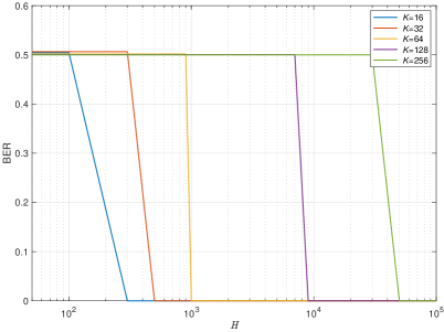
Figure 3: The defying performance of the proposed scheme for different values of $K$ and $H$.

The defying performance of our proposed defying scheme for different values of $K$ and $H$ is shown in Fig. 3. In this figure, we set $\theta_{0}=60^{\circ}$, $\theta_{e}=40^{\circ}$, $\Delta\tau=1/N$, $\{\tau_{n}^{o}\}_{n=1,2,...,N}=(n-1)/N$ and $\phi$ is taken as known. The SNR is set as $40$ dB. From Fig. 3, we can observe that the defying performance improves with $H$, as expected, and the BER can be reduced to $0$ even when $K=256$, demonstrating the great defying ability of our proposed scheme. Moreover, it can be seen that the defying scheme requires many more samples when $K$ is large. This is because a larger $K$ corresponds to a larger number of source signals, and thus ICA needs more samples to work well. Additionally, when $K$ is large and $|m|$ close to $K$, $V_{m}$ is very small due to the term $\operatorname{sinc}(m\pi\Delta\tau_{n})$ in (6). Considering that there are also estimation errors in ICA, for large $K$ and $|m|$ close to $K$, $|V_{m}|$ could be even smaller than the estimation errors of ICA, which will eventually lead to failure of the ambiguity resolving algorithm. Therefore, a large number of samples are needed to improve the accuracy of ICA estimates and accordingly the performance of the ambiguity resolving procedure.

V-B Efficiency of the Proposed Defying Scheme

Here, we compare the scrambling defying performance of our proposed CMICA against that of FastICA [40] for different numbers of OFDM symbols. We set $\theta_{0}=60^{\circ}$, $\theta_{e}=40^{\circ}$, $K=16$, and SNR=$40$ dB. We generate $30$ different groups of $\Delta\tau$ and $\{\tau_{n}^{o}\}_{n=1,2,...,N}$ randomly, according to the rules (C1)-(C3). The resulting BERs, averaged on these different groups of TMA parameters, are shown in Fig. 4. Based on this figure, we can see that the BER of both the CMICA-based defying scheme and the FastICA-based defying scheme decrease as $H$ increases. When $H$ is very large or very small, both methods perform similarly. However, the defied BER of CMICA reduces much faster and more significantly as $H$ increases, as compared to that of FastICA. The required $H$ for CMICA to defy the scrambling completely is around $10^{3}$, while that for FastICA is larger than $10^{4}$, suggesting a remarkable improvement of the sample utilization efficiency of CMICA. This improvement is consistent with the intuition revealed by the optimal non-Gaussinity invariance property shown in (18). Specifically, the gradual declining of defied BER with $H$ for both CMICA and FastICA implies that $\hat{J}_{G}(\boldsymbol{w})$ does not change abruptly with the sample length. When reducing the number of samples slowly from $D_{L}$ to $D_{S}$, $\hat{J}_{G}(\boldsymbol{w})$ will change accordingly but the optimal non-Gaussinity $\hat{J}_{G}(\boldsymbol{w}^{opt})$ does not change. So it is feasible to find $\boldsymbol{w}^{opt}$ even with $D_{S}$ for constant-modulus signals.

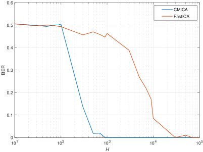
Figure 4: Comparison of the scrambling defying performance of CMICA and FastICA when using BPSK modulated data symbols.

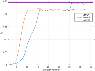
Figure 5: The level of non-Gaussianity with the ICA iteration number.

In Fig. 5, we examine how the two-stage iteration algorithm of CMICA behaves with $D_{S}$. Specifically, we compare the sum of $K$ non-Gaussianity values of CMICA and FastICA, respectively, against the iteration number when using fewer samples and illustrate the results in this figure, where $K=16$, $\theta_{0}=60^{\circ}$, $\theta_{e}=40^{\circ}$, $\Delta\tau=1/N$, $\{\tau_{n}^{o}\}_{n=1,2,...,N}=(n-1)/N$ and the maximal iteration number is set to $40$. For $D_{S}$, we set $n_{S}=H=1,000$. The values of non-Gaussianity are calculated based on (17), where $\boldsymbol{w}$ is obtained from each iteration of ICA. When $\boldsymbol{w}=\boldsymbol{w}^{opt}$, we obtain the optimal non-Gaussianity. From Fig. 5, it can be seen that the non-Gaussianity of CMICA converges first due to the Newton iteration and then due to the gradient descent iteration. The Newton iteration does not yield $\boldsymbol{w}^{opt}$, since the corresponding non-Gaussianity deviates from the optimal non-Gaussianity. However, after using the gradient descent, the non-Gaussianity of CMICA reaches the optimal $\boldsymbol{w}^{opt}$. In contrast, the FastICA fails to obtain the optimal non-Gaussianity after the iteration, indicating that FastICA cannot find $\boldsymbol{w}^{opt}$ when using $D_{S}$. This is because the decorrelation operation in FastICA is not applicable, as the statistical independence of $\boldsymbol{s}$ s is not maintained when using data of short length.

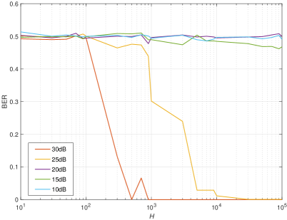
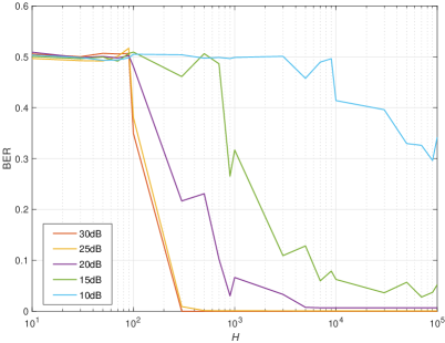
Figure 6: The scrambling defying performance with respect to the number of samples and the SNR: a) $k=1$ in the KNN-based ambiguity resolving scheme; b) $k=3$ in the KNN-based ambiguity resolving scheme.

V-C Robustness of the Proposed Defying Scheme

Finally, we provide simulation results to demonstrate the robustness of our proposed defying scheme to the receiver noise level. We examine the defied BER for different number of OFDM symbols and different noise levels, and showcase the results in Fig. 6. The SNR takes the values $(10,15,20,25,30)$ dB, $K=16$, $\theta_{0}=60^{\circ}$, $\theta_{e}=40^{\circ}$, $\Delta\tau=1/N$ and $\{\tau_{n}^{o}\}_{n=1,2,...,N}=(n-1)/N$. In Fig. 6 (a), $k=1$, and in Fig. 6 (b), $k=3$. From both Figs. 6 (a) and (b), we observe that the defied BER declines faster with higher SNRs when $H$ increases, meaning that the ICA estimation errors cannot be removed completely even after applying the Gaussian moments-based techniques [42] and the noise will affect the defying performance of the proposed scheme. With higher noise level, the ICA estimation errors increase, and accordingly, the performance of the ambiguity resolving algorithm degrades. As a result, the overall performance of the proposed defying scheme deteriorates at low SNRs. When comparing Figs. 6 (a) and (b), we can find that the defying performance with $k=3$ is better than that with $k=1$, especially for low SNRs. The reason behind improved robustness for lager $k$ is that the ICA estimation error will affect the mixing matrix reordering performance directly and then the reordering performance will influence the phase ambiguity resolving performance directly. At lower SNR, and accordingly higher ICA estimation error, the structure of the estimated mixing matrix will deviate more from the Toeplitz structure, and hence the reordering algorithm will fail to work. The wrongly reordered mixing matrix will further mislead the phase ambiguity resolving algorithm when there is only one candidate. So increasing the number of reordered mixing matrices as candidates can increase the defying robustness to the noise.

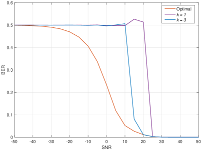
Figure 7: The defied BER of our proposed defying scheme for different SNR levels.

In Fig. 7, we compare the defied BER versus SNR for $k=1$ and $k=3$. We assume that the eavesdropper always knows the actual mixing matrix, so it can obtain the optimal defying performance, represented by ‘Optimal’ in Fig. 7. From this figure, it can be seen again that the defying performance when using $k=3$ outperforms that for $k=1$. Moreover, we can notice that the defied BER using our proposed scheme decreases abruptly with the SNR increasing, which is in contrast to the gradual descend of the optimal defied BER, and the defying performance is poor when the SNR is low. This indicates that the proposed defying scheme is sensitive to the high noise level and needs to be improved in further studies.

VI Conclusion

DM via TMAs transmitting OFDM waveforms has been viewed as an emerging hardware-efficient and low-complexity approach to secure wireless mobile communication systems. In this paper, we have presented, for the first time, a comprehensive assessment and analysis of wireless security of the DM transmitters via TMAs using OFDM waveforms. First, we have shown that this DM transmitter is not secure enough from the perspective of eavesdroppers. Specifically, we have formulated the defying of the TMA scrambling as a classical ICA problem for the eavesdropper, and shown that the ambiguities induced by ICA can be resolved by exploiting prior knowledge about the TMA OFDM system. For the ICA part, we have proposed an efficient ICA method, namely constant-modulus ICA (CMICA), that requires much fewer samples to obtain a good estimate of the mixing matrix by utilizing the constant modulus property. For the ambiguities, we construct a KNN-based resolving algorithm by exploiting jointly the Toeplitz structure of the mixing matrix, knowledge of data constellation, and the rules for designing the TMA ON-OFF pattern, etc. Then, we have showcased two kinds of conditions, for which the TMA OFDM systems are secure enough, and proposed some mechanisms that can be used to defend the scrambling against the attack of eavesdroppers. Through numerical results and analyses, we have demonstrated the effectiveness, efficiency, and robustness of our proposed defying and defending schemes in the end. Future studies will consider the extension of CMICA to other scenarios with constant-modulus signals. Also, the proposed defying scheme is promising to implement multiple-user DM simultaneously considering that the original TMA OFDM transmitter supports only single-user DM at a time.

References

- [1] A. D. Wyner, “The wire-tap channel,” Bell Syst. Tech. J, vol. 54, no. 8, pp. 1355–1387, Aug. 1975.
- [2] H. V. Poor and R. F. Schaefer, “Wireless physical layer security,” Proceedings of the National Academy of Sciences, vol. 114, no. 1, pp. 19–26, Jan. 2017.
- [3] B. Qiu, W. Cheng, and W. Zhang, “Decomposed and distributed directional modulation for secure wireless communication,” IEEE Tran. on Wire. Commun., vol. 23, no. 5, pp. 5219–5231, May 2023.
- [4] M. P. Daly and J. T. Bernhard, “Directional modulation technique for phased arrays,” IEEE Tran. on Ante. and Prop., vol. 57, no. 9, pp. 2633–2640, Sep. 2009.
- [5] N. Su, F. Liu, and C. Masouros, “Secure radar-communication systems with malicious targets: Integrating radar, communications and jamming functionalities,” IEEE Tran. on Wire. Commun., vol. 20, no. 1, pp. 83–95, 2022.
- [6] J. M. Purushothama, Y. Ding, G. Goussetis, G. Huang, and Y. Xiao, “Synthesis of energy efficiency-enhanced directional modulation transmitters,” IEEE Trans. on Green Comm. and Net., vol. 7, no. 2, pp. 635–648, June 2023.
- [7] L. Dong, Z. Han, A. P. Petropulu, and H. V. Poor, “Improving wireless physical layer security via cooperating relays,” IEEE Trans. on Signal Processing, vol. 58, no. 3, pp. 1875–1888, 2010.
- [8] J. Li, A. P. Petropulu, and S. Weber, “On cooperative relaying schemes for wireless physical layer security,” IEEE Trans. on Signal Processing, vol. 59, no. 10, pp. 4985–4997, 2011.
- [9] Q. Li and L. Yang, “Beamforming for cooperative secure transmission in cognitive two-way relay networks,” IEEE Trans. Inf. Forensics Security, vol. 15, pp. 130–143, 2020.
- [10] W. Zhang, J. Chen, Y. Kuo, and Y. Zhou, “Artificial-noise-aided optimal beamforming in layered physical layer security,” IEEE Commun. Lett., vol. 23, no. 1, pp. 72–75, 2019.
- [11] W. Wang, K. C. Teh, and K. H. Li, “Artificial noise aided physical layer security in multi-antenna small-cell networks,” IEEE Trans. Inf. Forensics Security, vol. 12, no. 6, pp. 1470–1482, 2017.
- [12] N. Su, F. Liu, Z. Wei, Y.-F. Liu, and C. Masouros, “Secure dual-functional radar-communication transmission: Exploiting interference for resilience against target eavesdropping,” IEEE Trans. on Wireless Communications, vol. 21, no. 9, pp. 7238–7252, 2022.
- [13] A. Kalantari, M. Soltanalian, S. Maleki, S. Chatzinotas, and B. Ottersten, “Directional modulation via symbol-level precoding: A way to enhance security,” IEEE J. Sel. Topics Signal Process., vol. 10, no. 8, pp. 1478–1493, Dec. 2016.
- [14] M. Alodeh, S. Chatzinotas, and B. Ottersten, “Energy-efficient symbol-level precoding in multiuser MISO based on relaxed detection region,” IEEE Tran. on Wire. Commun., vol. 15, no. 5, pp. 3755–3767, 2016.
- [15] M. R. Khandaker, C. Masouros, K.-K. Wong, and S. Timotheou, “Secure SWIPT by exploiting constructive interference and artificial noise,” IEEE Trans. on Communications, vol. 67, no. 2, pp. 1326–1340, 2018.
- [16] M. R. Khandaker, C. Masouros, and K.-K. Wong, “Constructive interference based secure precoding: A new dimension in physical layer security,” IEEE Trans. on Information Forensics and Security, vol. 13, no. 9, pp. 2256–2268, 2018.
- [17] N. Valliappan, A. Lozano, and R. W. Heath, “Antenna subset modulation for secure millimeter-wave wireless communication,” IEEE Trans. on Communications, vol. 61, no. 8, pp. 3231–3245, 2013.
- [18] Y. Ding, V. Fusco, and A. Chepala, “Circular directional modulation transmitter array,” IET Microw., Antennas and Propag., vol. 11, no. 3, pp. 1909–1917, Oct. 2017.
- [19] N. N. Alotaibi and K. A. Hamdi, “Switched phased-array transmission architecture for secure millimeter-wave wireless communication,” IEEE Trans. Commun., vol. 64, no. 3, pp. 1303–1312, Mar. 2016.
- [20] Y. Ding and V. Fusco, “A synthesis-free directional modulation transmitter using retrodirective array,” IEEE J. Sel. Topics Signal Process., vol. 11, no. 2, pp. 428–441, Mar. 2017.
- [21] G. Huang, S. Chen, Y. Ding, X. Li, A. Nallanathan, and S. Mumtaz, “Security-enhanced directional modulation symbol synthesis using high efficiency time-modulated arrays,” IEEE Trans. Veh. Tech., vol. 73, no. 1, pp. 1418–1423, Jan. 2024.
- [22] L. Manica, P. Rocca, L. Poli, and A. Massa, “Almost time-independent performance in time-modulated linear arrays,” IEEE Antennas and Wireless Propagation Letters, vol. 8, pp. 843–846, Jul. 2009.
- [23] P. Rocca, Q. Zhu, E. T. Bekele, S. Yang, and A. Massa, “4-d arrays as enabling technology for cognitive radio systems,” IEEE Trans. Antennas Propag., vol. 62, no. 3, pp. 1102–1116, Mar. 2014.
- [24] J. Guo, L. Poli, M. A. Hannan, P. Rocca, S. Yang, and A. Massa, “Time-modulated arrays for physical layer secure communications: Optimization-based synthesis and experimental assessment,” IEEE Trans. Antennas Propag., vol. 66, no. 12, pp. 6939–6949, Dec. 2018.
- [25] W. H. Kummer, A. T. Villeneuve, and F. G. Terrio, “New antenna idea - Scanning without phase shifters,” Electronics, vol. 36, no. 1, p. 27–32, Mar 1963.
- [26] W. H. Kummer, A. T. Villeneuve, T. S. Fong, and F. G. Terrio, “Ultra low sidelobes from time-modulated arrays,” IEEE Trans. Antennas Propag., vol. 11, no. 6, pp. 633–639, 1963.
- [27] Y. Ding, V. Fusco, J. Zhang, and W. Wang, “Time-modulated ofdm directional modulation transmitters,” IEEE Trans. Veh. Tech., vol. 68, no. 8, pp. 8249–8253, Aug. 2019.
- [28] S. Vosoughitabar, A. Nooraiepour, W. Bajwa, N. Mandayam, and C. Wu, “Metamaterial-enabled 2d directional modulation array transmitter for physical layer security in wireless communication links,” in 2022 IEEE/MTT-S International Microwave Symposium, Denver, CO, 2022.
- [29] S. Vosoughitabar, A. Nooraiepour, W. U. Bajwa, N. B. Mandayam, and C.-T. M. Wu, “Directional modulation retrodirective array-enabled physical layer secured transponder for protected wireless data acquisition,” in 2023 IEEE/MTT-S International Microwave Symposium-IMS, San Diego, CA, 2023, pp. 1180–1183.
- [30] A. Nooraiepour, S. Vosoughitabar, C.-T. M. Wu, W. U. Bajwa, and N. B. Mandayam, “Programming wireless security through learning-aided spatiotemporal digital coding metamaterial antenna,” Adv. Intell. Syst., vol. 5, no. 10, 2023.
- [31] G. Huang, Y. Ding, and S. Ouyang, “Multicarrier directional modulation symbol synthesis using time-modulated phased arrays,” IEEE Trans. Antennas Propag., vol. 20, no. 4, pp. 567–571, Apr. 2021.
- [32] G. Huang, Y. Ding, S. Ouyang, and J. M. Purushothama, “Target localization using time-modulated directional modulated transmitters,” IEEE Sensors J., vol. 22, no. 13, pp. 13 508–13 518, Jul. 2022.
- [33] Z. Xu and A. Petropulu, “A secure dual-function radar communication system via time-modulated arrays,” in Proc. IEEE RadarConf’23, San Antonio, TX, 2023.
- [34] ——, “Time-modulated intelligent reflecting surface for waveform security,” in Proc. IEEE Int. Conf. Acoust., Speech Signal Process. (ICASSP), Seoul, Korea, 2024.
- [35] A. Nooraiepour, S. Vosoughitabar, C.-T. M. Wu, W. U. Bajwa, and N. B. Mandayam, “Time-varying metamaterial-enabled directional modulation schemes for physical layer security in wireless communication links,” ACM Journal on Emerging Technologies in Computing Systems, vol. 18, no. 4, pp. 1–20, Oct. 2022.
- [36] H. Li, Y. Chen, and S. Yang, “Chaotic-enabled phase modulation in time-modulated arrays for secure transmission,” IEEE Trans. Antennas Propag., vol. 70, no. 11, pp. 10 454–10 464, Nov. 2022.
- [37] A. Hyvärinen and E. Oja, “Independent component analysis: Algorithms and applications,” Neural Networks, vol. 13, no. 4, pp. 411–430, Mar. 2000.
- [38] A. Hyvarinen, “Fast and robust fixed-point algorithms for independent component analysis,” IEEE Trans. on Neural Networks, vol. 10, no. 3, pp. 626–634, May 1999.
- [39] ——, “Independent component analysis: Recent advances,” Philos. Trans. Roy. Soc. A, Math., Phys. Eng. Sci., vol. 371, no. 1984, 2013.
- [40] E. Bingham and A. Hyvarinen, “A fast fixed-point algorithm for independent component analysis of complex valued signals,” Int. J. Neural Syst., vol. 10, pp. 1–8, 2000.
- [41] Z. Tao, Z. Xu, and A. Petropulu, “How secure is the time-modulated array-enabled ofdm directional modulation?” in Proc. IEEE Int. Conf. Acoust., Speech Signal Process. (ICASSP), Seoul, Korea, 2024.
- [42] A. Hyvarinen, “Fast ica for noisy data using gaussian moments,” in Proc. IEEE Int. Symp. Circuits Syst., vol. 5. IEEE, 1999, pp. 57–61.
- [43] H. Anton and C. Rorres, Elementary linear algebra: Aapplications version. John Wiley & Sons, 2013.