Continuous difference-in-differences with double/debiased machine learning

Abstract

This paper extends difference-in-differences to settings involving continuous treatments. Specifically, the average treatment effect on the treated (ATT) at any level of continuous treatment intensity is identified using a conditional parallel trends assumption. In this framework, estimating the ATTs requires first estimating infinite-dimensional nuisance parameters, especially the conditional density of the continuous treatment, which can introduce significant biases. To address this challenge, estimators for the causal parameters are proposed under the double/debiased machine learning framework. We show that these estimators are asymptotically normal and provide consistent variance estimators. To illustrate the effectiveness of our methods, we re-examine the study by Acemoglu and Finkelstein (2008), which assessed the effects of the 1983 Medicare Prospective Payment System (PPS) reform. By reinterpreting their research design using a difference-in-differences approach with continuous treatment, we nonparametrically estimate the treatment effects of the 1983 PPS reform, thereby providing a more detailed understanding of its impact.

Keywords: Difference-in-differences, causal inference, continuous treatment, machine learning

1 Introduction

Difference-in-differences (DiD) is one of the most popular research designs in empirical work. While the more common DiD settings focus on binary or discrete multi-valued treatments, there has been increasing interest in DiD with continuous treatments. The main idea of continuous DiD is simple: the treatment group rarely receives the treatment at the same level, and the treatment effect can vary with the “dose/intensity” of the treatment. Therefore, instead of comparing the outcomes of the treated and the controls before and after the treatment at the group level, one can further examine the treated group and compare the outcomes at different treatment intensities.

In fact, continuous treatment is prevalent in many empirical settings. For instance, each affected individual can have varied exposure to policy interventions, marketing campaigns, or environmental pollutants, all of which can be modeled as continuous treatments. Several recent studies in various fields have considered DiD with continuous treatments, including the study by Zeng et al. (2022) on the impact of shutting down online advertising sites, Cook et al. (2023)’s work on racial discrimination in public accommodations, and Ananat et al. (2022)’s study on the effects of the expanded child tax credit.

While continuous DiD is popular among empirical studies, its theoretical foundation is still limited. A few recent studies have started to fill this gap, notably Callaway et al. (2024), D’Haultfoeuille et al. (2023), and de Chaisemartin et al. (2022). For instance, Callaway et al. (2024) examine continuous DiD in the context of the commonly used two-way fixed effect (TWFE) regression setting. Concurrently, D’Haultfoeuille et al. (2023) generalize the change-in-changes model studied in Athey and Imbens (2006) to continuous treatment. On the other hand, de Chaisemartin et al. (2022) study the average slope of stayers in the continuous DiD setting. In contrast to these studies, our results build upon the semiparametric framework proposed in Abadie (2005), broadening its applicability to settings involving continuous treatments.

The main advantage of our approach is that it explicitly accounts for the presence of covariates and focuses directly on causal parameters: the average treatment effect on the treated (ATT) at any given continuous treatment intensity. As noted in Abadie (2005), the (unconditional) parallel trends assumption can be restrictive if there are covariates that affect outcome dynamics and their distributions differ between control and treatment groups. Therefore, we follow this same motivation and incorporate covariates nonparametrically into our identification and estimation strategy. One major difference that sets our results apart from Abadie (2005) is the presence of the continuous treatment, particularly its conditional density, which is commonly referred to as the “generalized propensity score” (see Hirano and Imbens (2004) for example). In this context, the causal parameter of interest, the ATT, becomes a function of the infinite-dimensional conditional density. This motivates us to consider the estimation and inference of the causal parameters under the double/debiased machine learning (DML) framework studied in Chernozhukov et al. (2018).

The estimation of the causal parameter requires first estimating nuisance parameters, including the conditional density of the continuous treatment. For potentially high-dimensional controls, researchers may want to use machine learning methods to estimate these nuisance parameters, which can result in substantial bias in the estimation of the causal parameter, see Chernozhukov et al. (2018) and the references therein for further examples. Moreover, if one estimates the nuisance parameters and the causal parameter using the same sample, another source of bias due to overfitting can also arise. To address these concerns, DML employs both an orthogonalization procedure and a cross-fitting procedure to reduce the influence of the nuisance parameters.

Due to the attractive properties of DML, we draw parallels with Chang (2020), which provides insights into DiD with discrete treatments under the DML framework, and extend the DML to our continuous DiD setting. Specifically, we first establish identification results analogous to Abadie (2005), but with continuous treatment. Notably, the propensity score of the treated group is replaced by the conditional density of the continuous treatment. We then derive orthogonal scores for both repeated outcomes (panel data) and repeated cross-sections settings, using a kernel function that concentrates on a specific continuous treatment intensity. Using these scores, we construct DML estimators of the ATTs and study their asymptotic properties. In particular, we show that our DML estimators are asymptotically normal, and the asymptotic bias vanishes with an undersmoothing kernel bandwidth. Moreover, we provide consistent variance estimators based on cross-fitting. The results from our carefully designed simulation studies suggest that our estimators perform well.

To illustrate the usefulness of our method, we revisit Acemoglu and Finkelstein (2008), which examines the impact of the 1983 Medicare payment system (PPS) reform on the heavily regulated healthcare industry. Since the PPS reform affected hospitals with varying proportions of Medicare inpatients differently, the share of Medicare inpatients can be interpreted as a continuous treatment variable. This makes Acemoglu and Finkelstein (2008) an exemplary case for applying our methods. Thus, we nonparametrically estimate the ATTs of the PPS reform in a continuous DiD context, providing a more detailed understanding of the effects of this policy reform. In particular, contrasting with the linear estimates from Acemoglu and Finkelstein (2008), our results suggest significant heterogeneity in the impact of the PPS reform across hospitals with different shares of Medicare inpatients.

The remainder of this paper is organized as follows. Section 2 introduces continuous DiD and demonstrates the identification of the causal parameter. Section 3 provides the orthogonal scores. In Section 4, we present our estimators and establish their asymptotic properties. Section 5 showcases the simulation results, followed by a detailed empirical example in Section 6. Finally, we conclude in Section 7.

2 Setup and Identification

In this section, we formally set up the difference-in-differences with continuous treatment following Abadie (2005). First, using the potential outcome notation (e.g. Rubin (1974)), let $Y_{i,t}(0)$ denote the potential outcome of individual $i$ in period $t$ when receiving no treatment, and similarly let $Y_{i,t}(d)$ denote the potential outcome of individual $i$ in period $t$ when receiving treatment with intensity $d$.

The treatment variable $D$ is modeled as a random variable with a mixture distribution: a probability mass at $0$ and a continuous distribution on an interval $[d_{L},d_{H}]$ excluding $0$. Specifically, the control group consists of individuals who receive treatment $D=0$, and we need a relatively large number of individuals in the control group so that the comparison between the treated and the control group is meaningful. On the other hand, the treated individuals can receive varied treatments, each with a potentially different treatment dose/intensity $D=d\in[d_{L},d_{H}]$ according to some continuous distribution. Moreover, we will assume throughout that the conditional probability $P(D=0|X)$ and density $f_{D|X}(d|X)$ for $d>0$ are well defined.

Remark 2.1.

To formalize the mixture distribution of the treatment variable, consider a measure $\nu=\delta_{0}+\lambda$, with $\lambda$ being the Lebesgue measure and $\delta_{0}$ being the Dirac delta at $0$. Suppose $F_{D}$ is the distribution of $D$. Then the density of $D$ w.r.t. $\nu$ is given by $dF_{D}/d\nu:=\mathbf{1}\{D=0\}P(D=0)+\mathbf{1}\{D>0\}f_{D}$ with $f_{D}$ being the probability density of $D$ on $[d_{L},d_{H}]$. In particular, $F_{D}(0)=\int\mathbf{1}\{D=0\}\frac{dF}{d\nu}d\nu=P(D=0)$ and for any measurable $A\in\mathcal{B}$ such that $0\notin A$, $F_{D}(D\in A)=\int_{A}f_{D}\ d\lambda$.

We restrict our attention to the two-period $(t-1,t)$ models and, as in the usual DiD setting, suppose that no subject receives treatment at period $0$, so we may suppress the time notation in treatment $D_{i}$. Let $X_{i}$ denote the set of individual-level covariates. We consider the following set of assumptions:

Assumption 2.1 (Repeated Outcomes).

The observed data $\{Y_{i,t-1},Y_{i,t},D_{i},X_{i}\}_{i=1}^{n}$ are independently and identically distributed.

Assumption 2.2 (Repeated Cross-Sections).

(a) For each individual $i$ in the pooled sample, the researcher observe $\{Y_{i},D_{i},X_{i},T_{i}\}$, where $T_{i}$ is a time indicator $=1$ if observation $i$ belongs to the post-treatment sample and $=0$ otherwise, and $Y_{i}=(1-T_{i})Y_{i,t-1}+T_{i}Y_{i,t}$; (b) (i) conditional on $T=0$, data are i.i.d. from the distribution of $(Y_{t-1},D,X)$; (ii) conditional on $T=1$, data are i.i.d. from the distribution of $(Y_{t},D,X)$.

Assumption 2.3 (Support).

(a) No subject receives treatment in the pre-treatment period; (b) the support of treatment $D$ satisfies $supp(D)=\{0\}\sqcup[d_{L},d_{H}]$ with $0<d_{L}<d_{H}\leq\infty$; (c) $P(D=0|X)>0$ almost surely; (d) $0<P(D=0)<1$ and $D$ admits a strictly positive probability density $f_{D}$ on $(d_{L},d_{H})$.

Assumption 2.4 (Conditional Parallel Trends).

For all $d\in[d_{L},d_{H}]$, the following holds

$$E[Y_{t}(0)-Y_{t-1}(0)|X,D=d]=E[Y_{t}(0)-Y_{t-1}(0)|X,D=0].$$

Assumptions 2.1 and 2.2 are standard in the DiD literature. In particular, Assumption 2.1 does not allow the covariates to vary over time, while Assumption 2.2(b) requires that the sample is not stratified by the outcome, treatment, or covariates. Moreover, Assumption 2.3 describes the requirements for the support of the treatment. Specifically, in the continuous DiD setting, the control group ($D=0$) must have a positive measure, and the treated group must have a positive likelihood of being treated at any intensity $d\in(d_{L},d_{H})$.

We want to emphasize the importance of Assumption 2.4, the conditional parallel trends condition that generalizes the discrete case of Abadie (2005), as the main identifying assumption that enables us to identify the causal parameter of interest. This assumption essentially states that, conditional on covariates, the unobserved counterfactual trend of the treated at each given treatment intensity is the same as the observed trend of the control group. In other words, the conditional parallel trends assumption allows us to substitute the unobserved counterfactual trend $E[Y_{t}(0)-Y_{t-1}(0)|X,D=d]$ by the observed trend $E[Y_{t}(0)-Y_{t-1}(0)|X,D=0]$ of the control group. Importantly, the extension of this assumption to the continuous treatment setting allows us to consider the heterogeneity in another dimension: the treatment intensity.

As commented in Abadie (2005), the covariates in DiD can serve two purposes, which also apply to our continuous treatment setting. First, covariates can be used to account for compositional differences between control and treatment groups that affect outcome dynamics. Moreover, covariates allow researchers to capture the heterogeneous treatment effects across different groups/individuals characterized by the covariates. In particular, the conditional parallel trends assumption allows us to explicitly incorporate the covariates in DiD nonparametrically, in contrast to commonly used parametric approaches in the literature, such as a linear model, which can potentially introduce misspecification biases.

Next, we describe our target parameter. The causal parameter we are interested in is the average treatment effect on the treated (ATT for short) at any given treatment intensity $d\in(d_{L},d_{H})$:

$$ATT(d):=E[Y_{t}(d)-Y_{t}(0)|D=d].$$ (2.1)

The interpretation of this parameter is analogous to the cases with discrete treatment variables: the expected effect of treatment with intensity $d$ for those who actually received treatment with intensity $d$. Note that ATT is a local measure, and in the absence of stronger assumptions, the average treatment effect $ATE(d):=E[Y_{t}(d)-Y_{t}(0)]$, which is the expected effect of treatment with intensity $d$ across the entire population, is not identified. The following theorem presents the main results of this section, in which we establish the identifications of $ATT(d)$ for both repeated outcomes and repeated cross-sections settings.

Theorem 2.1 (Identification of ATT).

(a) (Repeated Outcomes) If Assumptions 2.1, 2.3, and 2.4 hold, then, for any $d\in(d_{L},d_{H})$,

$$ATT(d)=E[Y_{t}-Y_{t-1}|D=d]-E\bigg{[}(Y_{t}-Y_{t-1})\mathbf{1}\{D=0\}\frac{f_{D|X}(d)}{f_{D}(d)P(D=0|X)}\bigg{]};$$ (2.2)

(b) (Repeated Cross-Sections) if Assumptions 2.2, 2.3, and 2.4 hold, then, for any $d\in(d_{L},d_{H})$,

$$ATT(d)=E\bigg{[}\frac{T-\lambda}{\lambda(1-\lambda)}Y|D=d\bigg{]}-E\bigg{[}\frac{T-\lambda}{\lambda(1-\lambda)}Y\mathbf{1}\{D=0\}\frac{f_{D|X}(d)}{f_{D}(d)P(D=0|X)}\bigg{]}$$ (2.3)

where $\lambda:=P(T=1)$.

Here we use the repeated outcomes case to illustrate the main idea. The proof for the repeated cross-sections case is similar and is deferred to the appendix. We begin by writing the ATT as

$$ATT(d)=E[Y_{t}(d)-Y_{t-1}(0)|D=d]-E[Y_{t}(0)-Y_{t-1}(0)|D=d].$$

First, by the modeling assumptions that $Y_{t}=Y_{t}(D)$ and $Y_{t-1}=Y_{t-1}(0)$ since no one receives treatment in the pre-treatment period, we have

$$E[Y_{t}(d)-Y_{t-1}(0)|D=d]=E[Y_{t}-Y_{t-1}|D=d].$$ (2.4)

Second, by the law of iterated expectation, Bayes’ rule, and conditional parallel trends assumption, we can express the counterfactual quantity as follows:

$$E[(Y_{t}(0)-Y_{t-1}(0))|D=d]$$

$$=\int E[(Y_{t}(0)-Y_{t-1}(0))|X=x,D=d]f_{X|D=d}(x)dx$$

$$=\int E[(Y_{t}(0)-Y_{t-1}(0))|X=x,D=d]\frac{f_{D|X}(d|x)f_{X}(x)}{f_{D}(d)}dx$$

$$=\int E[(Y_{t}(0)-Y_{t-1}(0))|X=x,D=0]\frac{f_{D|X}(d|x)f_{X}(x)}{f_{D}(d)}dx$$

$$=\int E[(Y_{t}(0)-Y_{t-1}(0))|X=x,D=0]\frac{f_{D|X}(d|x)P(D=0)}{f_{D}(d)P(D=0|X=x)}f_{X|D=0}(x)dx$$

$$=E\bigg{[}(Y_{t}-Y_{t-1})\mathbf{1}\{D=0\}\frac{f_{D|X}(d|X)}{f_{D}(d)P(D=0|X)}\bigg{]}.$$ (2.5)

Subtracting (2.5) from (2.4), we obtain the desired result. In particular, in the third equality in (2.5), we substitute the unobserved counterfactual trend $E[(Y_{t}(0)-Y_{t-1}(0))|X=x,D=d]$ by the observed trend $E[(Y_{t}(0)-Y_{t-1}(0))|X=x,D=0]$ of the control group, which is allowed by the conditional parallel trends assumption.

With Theorem 2.1, one can build estimators for $ATT(d)$ using the estimated sample analogs. For potentially high-dimensional covariates, machine learning methods can be employed to estimate the nuisance parameters, including the conditional density $f_{D|X}(d|X)$ and the conditional probability $P(D=0|X)$. However, the use of machine learning methods can often result in non-trivial first-order biases in the estimation of the causal parameter, which makes such “plug-in” estimators less desirable. One way to alleviate such biases is to consider alternative estimating equations that reduce the influence of the nuisance parameters on the causal parameters. We formalize this idea in detail in the next section.

3 Orthogonal Scores

In this section, we use the repeated outcomes case as our main example for illustration as the analogous discussion on repeated cross-sections only requires minor modifications. We begin by introducing the notion of Neyman orthogonality. For simplicity, consider the following notations: let $\theta_{0}\in\Theta\subset\mathbf{R}$ be the low-dimensional parameter of interest, e.g., $ATT(d)$ in our case; let $\rho_{0}\in\mathcal{H}$ denote the true low-dimensional nuisance parameters, e.g., in the repeated outcomes case, $\rho_{0}=f_{D}(d)$ for a given $d$; let $\eta_{0}\in\mathcal{T}$ denote the true infinite-dimensional nuisance parameters, which in our case include $f_{D|X}(d|X)$ and $P(D=0|X)$; let $\mathcal{T}_{n}\subset\mathcal{T}$ be a nuisance realization set in which the estimated $\hat{\eta}$ takes values with high probability; let $Z$ be the observable random vector, e.g. $Z=(Y_{t-1},Y_{t},D,X)$ in the repeated outcomes setting; let function $\psi:(Z,\theta,\rho,\eta)\mapsto\mathbf{R}$ denote a score.

With these notations, following Chernozhukov et al. (2018) and Chang (2020), we formally define the Neyman orthogonality with respect to the infinite-dimensional nuisance parameters:

Definition 1 (Neyman Orthogonality).

A score $\psi$ satisfies the Neyman orthogonality at $(\theta_{0},\rho_{0},\eta_{0})$ with respect to a nuisance realization set $\mathcal{T}_{n}\subset\mathcal{T}$ if (a) $\theta_{0}$ satisfies the moment condition

$$E_{P}[\psi(Z,\theta_{0},\rho_{0},\eta_{0})]=0;$$ (3.1)

(b) for $r\in[0,1)$ and $\eta\in\mathcal{T}_{n}$, the Gateaux (directional) derivative satisfies

$$\partial_{r}E_{P}[\psi(Z,\theta_{0},\rho_{0},\eta_{0}+r(\eta-\eta_{0}))]|_{r=0}=0.$$ (3.2)

In the above definition, (i) says that the score $\psi$ identifies the parameter of interests $\theta_{0}$ while (ii) ensures that the first-order bias from estimating the infinite-dimensional nuisance parameters is zero.

Recall that in the repeated outcomes case,

$$\theta_{0}=ATT(d)=E[\Delta Y|D=d]-E\bigg{[}\Delta Y\mathbf{1}\{D=0\}\frac{f_{D|X}(d|X)}{f_{D}(d)P(D=0|X)}\bigg{]}.$$ (3.3)

where $\Delta Y:=Y_{t}-Y_{t-1}$. This expression has two features that are worth noting. First, if $f_{D}(d)$ is estimated nonparametrically, e.g. using a kernel density estimator, we can no longer achieve root-$N$ rate when estimating $\theta_{0}$. The slower than root-$N$ rate appears to be a common feature in the literature that involves continuous treatment variables, see for example, Kennedy et al. (2017), Semenova and Chernozhukov (2021), and Colangelo and Lee (2022). Second, a score based on this expression does not satisfy Neyman orthogonality, and an adjustment term has to be added.

In general, the adjustment term is straightforward to construct if the nuisance parameters can be written as conditional expectations. However, in our case, while $P(D=0|X)$ can be expressed as a conditional expectation $E[\mathbf{1}\{D=0\}|X]$, the conditional density $f_{D|X}(d|X)$ presents additional challenges. To address this issue, we rely on the following observation (e.g., Fan et al. (1996)):

$$f_{D|X}(d|x)=\lim_{h\to 0}E[K_{h}(D-d)|X=x],\quad K_{h}(u):=\frac{1}{h}K\Big{(}\frac{u}{h}\Big{)}$$ (3.4)

where $K(\cdot)$ is a kernel function. The proof of this result can be established under mild regularity conditions and is given in the appendix. Replacing $f_{D|X}(d|x)$ by $E[K_{h}(D-d)|X=x]$, we define $ATT_{h}(d)$ as follows:

$$ATT_{h}(d):= E\bigg{[}\Delta Y\frac{K_{h}(D-d)}{f_{D}(d)}\bigg{]}-E\bigg{[}\Delta Y\mathbf{1}\{D=0\}\frac{E[K_{h}(D-d)|X]}{f_{D}(d)P(D=0|X)}\bigg{]}$$

$$= E\bigg{[}\Delta Y\frac{K_{h}(D-d)P(D=0|X)-\mathbf{1}\{D=0\}E[K_{h}(D-d)|X]}{f_{D}(d)P(D=0|X)}\bigg{]},$$ (3.5)

which is an expression that consists of only conditional expectations. Notably, it can be shown that

$$ATT(d)=\lim_{h\to 0}ATT_{h}(d),$$

which suggests that we can work with $ATT_{h}(d)$ instead. In particular, define the bias $B_{h}(d):=ATT_{d}-ATT_{h}(d)$, one can show that $B_{h}(d)=O(h^{2})$, and we defer the formal result and proof to the next section. For notation simplicity, we now formally define $ATT_{h}(d)$ in both settings.

Definition 2 (Repeated Outcomes).

$$ATT_{h}(d)=E\bigg{[}\Delta Y\frac{K_{h}(D-d)P(D=0|X)-\mathbf{1}\{D=0\}E[K_{h}(D-d)|X]}{f_{D}(d)P(D=0|X)}\bigg{]}$$ (3.6)

where $\Delta Y=Y_{t}-Y_{t-1}$.

Definition 3 (Repeated Cross-Sections).

$$ATT_{h}(d)= E\bigg{[}Y^{\lambda}\frac{K_{h}(D-d)P(D=0|X)-\mathbf{1}\{D=0\}E[K_{h}(D-d)|X]}{f_{D}(d)P(D=0|X)}\bigg{]}$$ (3.7)

where $Y^{\lambda}:=\frac{T-\lambda}{\lambda(1-\lambda)}Y$.

Our goal is to construct a score that satisfies Neyman orthogonality for each $h$, and then take the limit as $h\to 0$. The next lemma presents such scores. To simplify the expressions, denote: $g(X):=P(D=0|X)$; $f_{h}(d|X):=E[K_{h}(D-d)|X]$; $\mathcal{E}_{\Delta Y}(X):=E[\Delta Y|X,D=0]$; $\mathcal{E}_{\lambda Y}(X):=E\big{[}\frac{T-\lambda}{\lambda(1-\lambda)}Y|X,D=0\big{]}$ with $\lambda=P(T=1)$; $f_{d}:=f_{D}(d)$.

Lemma 3.1.

Suppose there exist $M_{h}^{(1)}\in L^{1}(P_{Y_{t-1},Y_{t},D,X})$ and $M_{h}^{(2)}\in L^{1}(P_{Y,T,D,X})$ such that $|\psi_{h}^{(1)}|\leq M_{h}^{(1)}$ and $|\psi_{h}^{(2)}|\leq M_{h}^{(2)}$ almost surely. Then the scores $\psi_{h}^{(1)}$ and $\psi_{h}^{(2)}$ satisfy Neyman orthogonality defined in (1), where (a) for the repeated outcomes setting,

$$\psi_{h}^{(1)}:=\frac{K_{h}(D-d)g(X)-\mathbf{1}\{D=0\}f_{h}(d|X)}{f_{D}(d)g(X)}\bigg{(}\Delta Y-\mathcal{E}_{\Delta Y}(X)\bigg{)}-ATT_{h}(d);$$ (3.8)

(b) for the repeated cross-sections setting,

$$\psi_{h}^{(2)}:=\frac{K_{h}(D-d)g(X)-\mathbf{1}\{D=0\}f_{h}(d|X)}{f_{D}(d)g(X)}\bigg{(}\frac{T-\lambda}{\lambda(1-\lambda)}Y-\mathcal{E}_{\lambda Y}(X)\bigg{)}-ATT_{h}(d).$$ (3.9)

The proof is given in the appendix, in which we explain the construction of the adjustment term and verify the Neyman orthogonality conditions given in Definition 1. The assumption on the existence of integrable functions $M_{h}^{(1)}$ and $M_{h}^{(2)}$ is a mild regularity condition that allows us to interchange expectation and derivative. This assumption can be readily checked under the boundedness of the nuisance parameters in the scores, which will be made precise in the next section. For notational simplicity, we drop the superscripts on $\psi^{(1)}_{h}$ and $\psi^{(2)}_{h}$ whenever the context is clear.

We note that in these new scores, the infinite-dimensional nuisance parameters are $f_{h}(d|X)$, $g(X)$, $\mathcal{E}_{\Delta Y}(X)$, and $\mathcal{E}_{\lambda Y}(X)$, with the latter two being the new ones created when constructing the adjustment terms. In particular, the estimating moments for $ATT_{h}(d)$’s based on these orthogonal scores are not sensitive to potentially biased estimates of these nuisance parameters. In the next section, we will construct DML estimators of $ATT_{h}(d)$’s using these scores and establish their asymptotic properties.

4 Estimation and Inference

As mentioned in the introduction, constructing DML estimators involves two main steps. In the previous section, we addressed the first step by establishing scores that satisfy Neyman orthogonality, as detailed in Lemma 3.1. These scores are then utilized in conjunction with the second critical aspect of DML estimators — the cross-fitting techniques. These techniques aim to reduce the overfitting bias that arises when estimating nuisance parameters using machine learning methods. With these key components in place, we can construct DML estimators following the procedure proposed by Chernozhukov et al. (2018).

First, we partition the random sample $I_{N}$ into $K\geq 2$ disjoint subsets $\{I_{k}\}_{k=1}^{K}$ of equal size $n=N/K$. Then, for each $k\in\{1,\cdots,K\}$, we use the sample $I_{k}^{c}:=I_{N}\setminus I_{k}$ to estimate the nuisance parameters with the preferred machine learning methods. Next, we compute sample averages according to (3.6)/(3.7) using the estimated nuisance parameters evaluated at the sample $I_{k}$ to obtain the $k$-th estimate $\widehat{ATT}_{k}(d)$ for $ATT(d)$. Finally, we average through the $K$ estimates to obtain the final estimator. The following algorithms summarize the procedure.

Algorithm 1 (CDID Estimator, Repeated Outcomes).

Let $\{I_{k}\}_{k=1}^{K}$ denote a partition of a random sample $\{(Y_{i,t-1},Y_{i,t},D_{i},X_{i}\}_{i=1}^{N}$, each with equal size $n=N/K$, and for each $k\in\{1,\cdots,K\}$, let $I_{k}^{c}:=I_{N}\setminus I_{k}$ denote the complement.

• For each $k$, construct

  $$\widehat{ATT}_{k}(d) :=\frac{1}{n}\sum_{i\in I_{k}}\frac{K_{h}(D_{i}-d)\hat{g}_{k}(X_{i})-\mathbf{1}\{D_{i}=0\}\hat{f}_{h,k}(d|X_{i})}{\hat{f}_{d,k}\hat{g}_{k}(X_{i})}\big{(}\Delta Y_{i}-\hat{\mathcal{E}}_{\Delta Y,k}(X_{i})\big{)}$$

  where $\hat{f}_{d,k},\hat{f}_{h,k},\hat{g}_{k},\hat{\mathcal{E}}_{\Delta Y,k}$ are the estimators of $f_{d},f_{h}(d|X),g(X)$ and $\mathcal{E}_{\Delta Y}(X)$ respectively using the rest of the sample $I_{k}^{c}$. In particular, $\hat{f}_{d,k}$ is a kernel density estimator, and $\hat{f}_{h,k}$, $\hat{g}_{k}$ and $\hat{\mathcal{E}}_{\Delta Y,k}$ are estimated using ML methods (e.g. random forests or deep neural networks).

• Average through the $K$ estimators to obtain the final estimator

  $$\widehat{ATT}(d):=\frac{1}{K}\sum_{k=1}^{K}\widehat{ATT}_{k}(d).$$

Algorithm 2 (CDID Estimator, Repeated Cross-Sections).

Let $\{I_{k}\}_{k=1}^{K}$ denote a partition of a random sample $\{(Y_{i,t-1},Y_{i,t},D_{i},X_{i}\}_{i=1}^{N}$, each with equal size $n=N/K$, and for each $k\in\{1,\cdots,K\}$, let $I_{k}^{c}:=I_{N}\setminus I_{k}$ denote the complement.

• For each $k$, construct

  $$\widehat{ATT}_{k}(d):=\frac{1}{n}\sum_{i\in I_{k}} \frac{K_{h}(D_{i}-d)\hat{g}_{k}(X_{i})-\mathbf{1}\{D_{i}=0\}\hat{f}_{h,k}(d|X_{i})}{\hat{f}_{d,k}\hat{g}_{k}(X_{i})}$$

  $$\times\bigg{(}\frac{T_{i}-\hat{\lambda}_{k}}{\hat{\lambda}_{k}(1-\hat{\lambda}_{k})}Y_{i}-\hat{\mathcal{E}}_{\lambda Y,k}(X_{i})\bigg{)}$$

  where $\hat{f}_{d,k},\hat{f}_{h,k},\hat{g}_{k},\hat{\mathcal{E}}_{\lambda Y,k}$ are the estimators of $f_{d},f_{h}(d|X),g(X)$ and $\mathcal{E}_{\lambda Y}(X)$ respectively using the rest of the sample $I_{k}^{c}$. In particular, $\hat{f}_{d,k}$ is a kernel density estimator, and $\hat{f}_{h,k}$, $\hat{g}_{k}$ and $\hat{\mathcal{E}}_{\Delta Y,k}$ are estimated using ML methods (e.g. random forests or deep neural networks).

• Average through the $K$ estimators to obtain the final estimator

  $$\widehat{ATT}(d):=\frac{1}{K}\sum_{k=1}^{K}\widehat{ATT}_{k}(d).$$

Remark 4.2.

It is important to note that at each $k=1,\cdots,K$, the nuisance parameters and the $\widehat{ATT}_{k}(d)$ are estimated using disjoint subsamples. While doing so helps reduce the overfitting bias, the sample splitting also significantly simplifies the asymptotic analysis, which itself has a long history in the literature (see Chernozhukov et al. (2018) and references therein). Moreover, the cross-fitting ensures that the final estimator uses the full sample, and hence the choice of $K$ does not affect the asymptotic analysis of our estimator. In practice, we recommend using $K=5$ as a rule of thumb.

Next, we state regularity conditions that allow us to prove the asymptotic normality of our DML estimators.

Assumption 4.5 (Kernel).

The kernel function $K(\cdot)$ satisfies: (a) $K(\cdot)$ is bounded and differentiable; (b) $\int K(u)du=1$, $\int uK(u)du=0$, $0<\int u^{2}K(u)du<\infty$. Moreover, for notational simplicity, define $K_{h}(u):=h^{-1}K(u/h)$.

Assumption 4.6 (Bounds and Smoothness, Repeated Outcomes).

(a) For some constants $0<c<1$ and $0<C<\infty$, $f_{d}>c$, $|Y_{t-1}|<C$, $|Y_{t}|<C$, $|f_{h}(d|X)|<C$, and $|\mathcal{E}_{\Delta Y}(X)|<C$ almost surely; (b) for some constants $0<\kappa<\frac{1}{2}$ and for all $h>0$, $\kappa<g(X)<1-\kappa$ almost surely; (c) $f_{d}\in C^{2}((d_{L},d_{H}))$ and $|f_{d}^{(2)}|<\infty$; (d) $f_{D|X}(d|x)\in C^{2}((d_{L},d_{H}))$ and $\sup_{x\in\text{supp}(X)}|f_{D|X}^{(2)}(d|x)|<\infty$; (e) joint density $f_{\Delta Y,D}(t,d)\in C^{2}(\text{supp}(\Delta Y))$ and $\sup_{d\in(d_{L},d_{H})}|f_{\Delta Y,D}^{(2)}(t,d)|<\infty$.

Assumption 4.7 (Rates, Repeated Outcomes).

(a) The kernel bandwidth $h$ is a deterministic sequence that depends on $N$ and satisfies $Nh\to\infty$ and $\sqrt{Nh^{5}}=o(1)$; (b) there exists a sequence $\varepsilon_{N}\to 0$ such that $h^{-1}\varepsilon_{N}^{2}=o(1)$; (c) with probability tending to $1$, $\|\hat{f}_{h}(d|X)-f_{h}(d|X)\|_{P,2}\leq h^{-1/2}\varepsilon_{N}$, $\|\hat{g}(X)-g(X)\|_{P,2}\leq\varepsilon_{N}$, $\|\hat{\mathcal{E}}_{\Delta Y}(X)-\mathcal{E}_{\Delta Y}(X)\|_{P,2}\leq\varepsilon_{N}$; (d) with probability tending to $1$, $\kappa<\|\hat{g}(X)\|_{P,\infty}<1-\kappa$, $\|\hat{f}_{h}(d|X)\|_{P,\infty}<C$, and $\|\hat{\mathcal{E}}_{\Delta Y}(X)\|_{P,\infty}<C$.

Assumption 4.8 (Bounds and Smoothness, Repeated Cross-Sections).

(a) For some constants $0<c<1$ and $0<C<\infty$, $f_{d}>c$, $c<\lambda<1-c$, $|Y|<C$, $|f_{h}(d|X)|<C$, and $|\mathcal{E}_{\lambda Y}(X)|<C$ almost surely; (b) for some constants $0<\kappa<\frac{1}{2}$ and for all $h>0$, $\kappa<g(X)<1-\kappa$ almost surely; (c) $f_{d}\in C^{2}((d_{L},d_{H}))$ and $|f_{d}^{(2)}|<\infty$; (d) $f_{D|X}(d|x)\in C^{2}((d_{L},d_{H}))$ and $\sup_{x\in\text{supp}(X)}|f_{D|X}^{(2)}(d|x)|<\infty$; (e) joint density $f_{Y^{\lambda},D}(t,d)\in C^{2}(\text{supp}(Y^{\lambda}))$ and $\sup_{d\in(d_{L},d_{H})}|f_{Y^{\lambda},D}^{(2)}(t,d)|<\infty$.

Assumption 4.9 (Rates, Repeated Cross-Sections).

(a) The kernel bandwidth $h$ is a deterministic sequence that depends on $N$ and satisfies $Nh\to\infty$ and $\sqrt{Nh^{5}}=o(1)$; (b) there exists a sequence $\varepsilon_{N}\to 0$ such that $h^{-1}\varepsilon_{N}^{2}=o(1)$; (c) with probability tending to $1$, $\|\hat{f}_{h}(d|X)-f_{h}(d|X)\|_{P,2}\leq h^{-1/2}\varepsilon_{N}$, $\|\hat{g}(X)-g(X)\|_{P,2}\leq\varepsilon_{N}$, $\|\hat{\mathcal{E}}_{\lambda Y}(X)-\mathcal{E}_{\lambda Y}(X)\|_{P,2}\leq\varepsilon_{N}$; (d) with probability tending to $1$, $\kappa<\|\hat{g}(X)\|_{P,\infty}<1-\kappa$, $\|\hat{f}_{h}(d|X)\|_{P,\infty}<C$, and $\|\hat{\mathcal{E}}_{\lambda Y}(X)\|_{P,\infty}<C$.

The kernel function plays a central role in our analysis. Not only do we use the kernel to estimate the low-dimensional parameter $f_{D}(d)$ given its well-established theoretical properties, but we also use the kernel to approximate the point mass at $D=d$ as well as the conditional density $f_{D|X}(d|X)$. In Assumption 4.5, we assume the standard regularity conditions for the kernel function, which are crucial for establishing the asymptotic normality of our estimator and are easy to verify. Moreover, Assumptions 4.6, 4.8 impose bounds and smoothness conditions on the outcome variable and distributions/conditional distributions. In addition, Assumptions 4.7, 4.9 impose restrictions on the kernel bandwidth as well as the quality of the nonparametric estimators of nuisance parameters: (a) and (b) require the kernel bandwidth $h$ to be under-smoothing (but not too much) so that the bias vanishes asymptotically (otherwise asymptotic normality still holds but not centered at $\theta_{0}$); (c) assumes the estimators of the nuisance parameters to satisfy certain rates of convergence; and (d) ensures that such estimators are bounded.

Remark 4.3.

First, if $\varepsilon_{N}=o(N^{-1/4})$, then Assumption 4.7 (i) and (ii) together imply that $h=o(N^{-1/5})$ and $h\geq O(N^{-1/2})$. However, as we will see shortly, in order to show the consistency of the variance estimator, we need to assume additionally that $h^{-2}\varepsilon_{N}^{2}=o(1)$. This suggests that we need an under-smoothing kernel bandwidth $h$ but we cannot under-smooth too much. Second, while the DML literature typically assumes that the estimators of the nuisance parameters converge at rate $\varepsilon_{N}=o(N^{-1/4})$, see Chernozhukov et al. (2018) for example, we allow the conditional density $\hat{f}_{h}$ to converge at an even slower rate. This does not contradict the existing DML literature since the estimator for our target parameter can not achieve $\sqrt{N}$ rate due to the presence of a continuous treatment variable.

Before stating the main theorems of this section, we first introduce a lemma that characterizes the bias $ATT(d)-ATT_{h}(d)$ in terms of the kernel bandwidth $h$.

Lemma 4.2 (Bias of $ATT_{h}(d)$).

Suppose Assumptions 4.5, 4.6, 4.7 hold for the repeated outcomes case, and Assumptions 4.5, 4.8, 4.9 hold for the repeated cross-sections case. Then $B_{h}(d):=ATT(d)-ATT_{h}(d)$ satisfies $B_{h}(d)=O(h^{2})$ for any $d\in(d_{L},d_{H})$.

The proof is given in the appendix. This lemma suggests that the bias from the kernel approximation can be controlled by choosing an appropriate bandwidth. In particular, for an under-smoothing bandwidth, the bias does not affect the asymptotic distribution of our estimators. The next theorem is the main result of this section that establishes the asymptotic normality of our estimators for $ATT(d)$.

Theorem 4.2 (Asymptotic Normality).

(a) (Repeated Outcomes) Suppose assumptions 2.1, 2.3, 2.4, 4.5, 4.6, and 4.7 hold. Then

$$\frac{\widehat{ATT}(d)-ATT(d)}{\sigma_{1N}/\sqrt{N}}\quad\to^{d}\quad N(0,1)$$

where

$$\sigma_{1N}^{2}:=E\bigg{[}\bigg{(}\psi_{h}^{(1)}(Z,\theta_{0h},f_{d}^{0},\eta_{0})-\frac{\theta_{0h}}{f_{d}^{0}}\big{(}K_{h}(D-d)-E[K_{h}(D-d)]\big{)}\bigg{)}^{2}\bigg{]}$$ (4.1)

for $\theta_{0h}:=ATT_{h}(d)$ defined as in (3.6) and $\psi_{h}^{(1)}$ defined as in (3.8); (b) (Repeated Cross-Sections) Suppose assumptions 2.2, 2.3, 2.4, 4.5, 4.8, and 4.9 hold. Then

$$\frac{\widehat{ATT}(d)-ATT(d)}{\sigma_{2N}/\sqrt{N}}\quad\to^{d}\quad N(0,1)$$

where

$$\sigma_{2N}^{2}:=E\bigg{[}\bigg{(}\psi_{h}^{(2)}(Z,\theta_{0h},\lambda_{0},f_{d}^{0},\eta_{0})-\frac{\theta_{0h}}{f_{d}^{0}}\big{(}K_{h}(D-d)-E[K_{h}(D-d)]\big{)}\bigg{)}^{2}\bigg{]}$$ (4.2)

for $\theta_{0h}:=ATT_{h}(d)$ defined as in (3.7) and $\psi_{h}^{(2)}$ defined as in (3.9).

The proof follows the general framework for DML estimators studied in Chernozhukov et al. (2018) with modifications to accommodate the presence of kernel functions. The asymptotic variance roughly consists of two parts that contribute to the slower than $\sqrt{N}$ rate: the part from the orthogonal score $\psi_{h}$ that grows with $h$ and the part from the kernel used to nonparametrically estimate the density $f_{D}(d)$. Under the assumptions, our estimator $\widehat{ATT}(d)$ converges at rate $\sqrt{Nh}$, which is slower than the parametric rate $\sqrt{N}$ but comparable to the optimal rate for 1-dimensional nonparametric estimation.

In practice, to establish a point-wise confidence interval for $ATT(d)$, we need consistent estimators for the asymptotic variances established in the theorem. Following Chernozhukov et al. (2018) and Chang (2020), we consider the following cross-fitted variance estimators. For notational simplicity, we use $\hat{\theta}_{h}:=\widehat{ATT}(d)$ to denote our cross-validated estimators, and $E_{n,k}$ to denote the empirical average using the subsample $I_{k}$. For the repeated outcomes case, define

$$\hat{\sigma}_{1N}^{2}:=\frac{1}{K}\sum_{k=1}^{K}E_{n,k}\bigg{[}\bigg{(}\psi_{h}^{(1)}(Z,\hat{\theta}_{h},\hat{f}_{d,k},\hat{\eta}_{k})-\frac{\hat{\theta}_{h}}{\hat{f}_{d,k}}\big{(}K_{h}(D-d)-\hat{f}_{d,k}\big{)}\bigg{)}^{2}\bigg{]}.$$ (4.3)

Similarly, for the repeated cross-sections case, define

$$\hat{\sigma}_{2N}^{2}:=\frac{1}{K}\sum_{k=1}^{K}E_{n,k}\bigg{[}\bigg{(}\psi_{h}^{(2)}(Z,\hat{\theta}_{h},\hat{\lambda}_{k},\hat{f}_{d,k},\hat{\eta}_{k})-\frac{\hat{\theta}_{h}}{\hat{f}_{d,k}}\big{(}K_{h}(D-d)-\hat{f}_{d,k}\big{)}\bigg{)}^{2}\bigg{]}.$$ (4.4)

Then, with these variance estimators, the $1-\alpha$ confidence interval can be constructed as $[\widehat{ATT}(d)-z_{1-\alpha/2}\hat{\sigma}_{N}/\sqrt{N},\widehat{ATT}(d)+z_{1-\alpha/2}\hat{\sigma}_{N}/\sqrt{N}]$ where $z_{1-\alpha/2}$ denotes the $1-\alpha/2$ quantile of the standard normal random variable. The following theorem establishes the consistency of the cross-fitted variance estimators for both settings.

Theorem 4.3.

Suppose assumptions in Theorem 4.2 hold. In addition, assume that $h^{-2}\varepsilon_{N}^{2}=o(1)$. Then (a) for the repeated outcomes case,

$$\hat{\sigma}_{1N}^{2}=\sigma_{1N}^{2}+o_{p}(1)$$

where $\hat{\sigma}_{1N}^{2}$ is defined as in (4.3) and $\sigma_{1N}^{2}$ is defined as in (4.1); (b) for the repeated cross-sections case,

$$\hat{\sigma}_{2N}^{2}=\sigma_{2N}^{2}+o_{p}(1)$$

where $\hat{\sigma}_{2N}^{2}$ is defined as in (4.4) and $\sigma_{2N}^{2}$ is defined as in (4.2).

Alternatively, we can consider a multiplier bootstrap procedure to construct confidence intervals. Notably, such procedure has been discussed extensively in recent studies, see, e.g., Belloni et al. (2017), Su et al. (2019), Cattaneo and Jansson (2021), Colangelo and Lee (2022), and Fan et al. (2022). Specifically, let $\{\xi_{i}\}_{i=1}^{N}$ be an i.i.d. sequence of sub-exponential random variables independent of $\{Y_{i,t-1},Y_{i,t},D_{i},X_{i}\}_{i=1}^{N}$ for repeated outcomes case, or independent of $\{Y_{i},T_{i},D_{i},X_{i}\}_{i=1}^{N}$ for repeated cross-sections case, such that $E[\xi_{i}]=Var(\xi_{i})=1$. Then for each $b=1,\cdots,B$, we draw such a sequence $\{\xi_{i}\}_{i=1}^{N}$ and construct estimates based on the following expressions.

For the repeated outcomes, define

$$\widehat{ATT}(d)_{b}^{*}:=\frac{1}{N}\sum_{k=1}^{K}\sum_{i\in I_{k}}\xi_{i} \frac{K_{h}(D_{i}-d)\hat{g}_{k}(X_{i})-\mathbf{1}\{D_{i}=0\}\hat{f}_{h,k}(d|X_{i})}{\hat{f}_{d,k}\hat{g}_{k}(X_{i})}$$

$$\times \big{(}\Delta Y_{i}-\hat{\mathcal{E}}_{\Delta Y,k}(X_{i})\big{)}.$$ (4.5)

Similarly, for the repeated cross-sections, define

$$\widehat{ATT}(d)_{b}^{*}:=\frac{1}{N}\sum_{k=1}^{K}\sum_{i\in I_{k}}\xi_{i} \frac{K_{h}(D_{i}-d)\hat{g}_{k}(X_{i})-\mathbf{1}\{D_{i}=0\}\hat{f}_{h,k}(d|X_{i})}{\hat{f}_{d,k}\hat{g}_{k}(X_{i})}$$

$$\times \bigg{(}\frac{T_{i}-\hat{\lambda}_{k}}{\hat{\lambda}_{k}(1-\hat{\lambda}_{k})}Y_{i}-\hat{\mathcal{E}}_{\lambda Y,k}(X_{i})\bigg{)}.$$ (4.6)

Let $\hat{c}_{\alpha}$ denote the $\alpha$’s quantile of $\{\widehat{ATT}(d)_{b}^{*}-\widehat{ATT}(d)\}_{b=1}^{B}$, a $1-\alpha$ confidence interval can be constructed as $[\widehat{ATT}(d)-\hat{c}_{1-\alpha/2},\widehat{ATT}(d)-\hat{c}_{\alpha/2}]$. We defer the theoretical discussions of this procedure to future work.

5 Simulation

In this section, we present the Monte Carlo simulation results for both the repeated outcomes and repeated cross-sections settings. We provide a brief overview of the data-generating process and the estimation procedure for the nuisance parameters in the repeated outcomes setting. Additional details are provided in the appendix.

Data-generating process, repeated outcomes setting: (a) $p=100$ dimensional covariates $X\sim N(0,\Sigma)$, where the covariance matrix $\Sigma$ has variances equal to $1$ on the diagonal and covariances equal to $0.1$ on the off-diagonal; (b) the propensity score for the control group is generated according to $P(D=0|X)=1/(1+\exp(-X^{\prime}\gamma))$, with $\gamma_{j}=0.5j^{-2}$; (c) for the treatment group $D>0$, the continuous treatment is generated according to $D|X,V\sim\text{Exp}(|X^{\prime}\alpha+V|)$, where $V\perp X$, $V\sim N(0,1)$, $\alpha_{j}=0.3j^{-2}$; (d) the potential outcomes are generated according to $Y_{t-1}(0)=\epsilon_{1}$, $Y_{t}(0)=Y_{t-1}(0)+X^{\prime}\beta+1+\epsilon_{2}$, $Y_{t}(D)=Y_{t}(0)-0.5D^{2}+\epsilon_{3}$, where $\beta_{j}=0.5/j$ for $j=1,\cdots,6$ and $0$ otherwise, and all the errors $\epsilon_{1},\epsilon_{2},\epsilon_{3}$ have independent standard normal distributions. The observed data are $(Y_{i,t-1},Y_{i,t},X_{i},D_{i})$, with $Y_{t-1}=Y_{t-1}(0)$ and $Y_{t}=1{D>0}Y_{t}(D)+1{D=0}Y_{t}(0)$.

In our simulations, the propensity score for the control group $P(D=0|X)$ is estimated using cross-validated Logit LASSO, the conditional density $f_{h}(d|X)=E[K_{h}(D-d)|X]$ is estimated nonparametrically using random forests, and the remaining nuisance parameter $E[Y_{t}-Y_{t-1}|X,D=0]$ is estimated using cross-validated LASSO. We also use an undersmoothing kernel bandwidth $h=0.5N^{-4}$ throughout our simulations.

The DGP implies the true $ATT(d)=-0.5d^{2}$, and we focus on a specific treatment intensity $d=0.9$. The histograms of the simulation estimates are shown in Figure 1, where the red lines indicate the true ATT. We observe that as the sample size increases, both the bias and variance decrease. This demonstrates that our estimator performs well even with the highly non-linear relationship between the continuous treatment variable and high-dimensional covariates. Notably, the conditional density with 100 covariates is approximated by a kernel conditional mean $E[K_{h}(D-d)|X]$, which is estimated nonparametrically using machine learning methods. Despite the relatively small sample size in our simulation, this approach to estimating the conditional density performs well in our setting. Furthermore, the undersmoothing kernel bandwidth effectively reduces the asymptotic bias, as predicted by the theory.

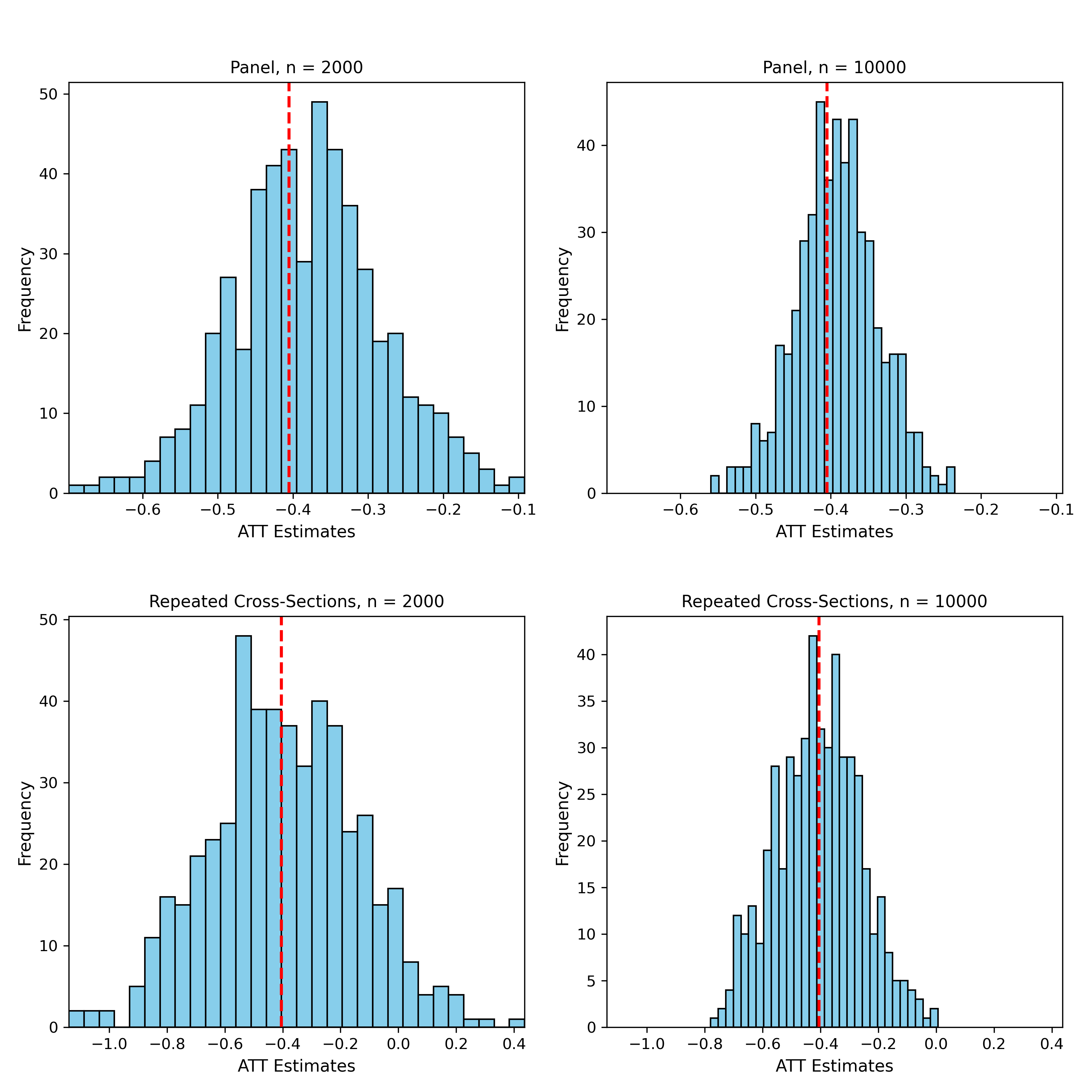
Figure 1: The simulation results, true $ATT(d)=0.405$.

6 Empirical Example

6.1 Background

The Medicare Prospective Payment System (PPS) reform, introduced in 1983, changed the way Medicare reimburses hospitals for inpatient care. Instead of a full-cost reimbursement model based on actual expenses, hospitals began receiving a predetermined amount per patient based on the diagnosis. Notably, during the first three years post-reform, reimbursements for capital costs still reflected actual expenses. This meant that hospitals treating Medicare patients experienced a relative increase in labor costs compared to capital costs. Acemoglu and Finkelstein (2008) highlighted this unique aspect of the PPS reform, and their research revealed that the PPS reform not only significantly raised the capital-labor ratio in hospitals but also promoted the adoption of new technologies.

Specifically, one of the main theoretical predictions in Acemoglu and Finkelstein (2008) posits that the PPS reform would result in a higher capital-labor ratio in hospitals. Moreover, if the elasticity of substitution between capital and labor is sufficiently large, PPS reform should lead to an increase in demand for capital/technology. It is important to note that, since only hospitals with Medicare patients are affected by this reform, these effects could be different for hospitals with varying shares of Medicare patients. To test these predictions empirically, Acemoglu and Finkelstein (2008) uses data from the Annual American Hospital Association (AHA) survey of hospitals from 1980 to 1986, which contains information on hospital expenditure, employment, and other characteristics related to the technologies at the hospital level.

The baseline specification in Acemoglu and Finkelstein (2008) takes the following form of a linear regression:

$$Y_{i,t}=\alpha_{i}+\gamma_{t}+X_{i,t}^{\prime}\eta+\beta\cdot(D_{i}\cdot\text{Post}_{t})+\varepsilon_{i,t},$$ (6.1)

where $Y_{i,t}$ denotes either the capital-labor ratio or the total number of medical facilities of hospital $i$ in year $t$, $D_{i}$ denotes the share of Medicare inpatient days in hospital $i$ prior to the PPS reform, $\text{Post}_{t}=\mathbf{1}\{t\in\text{post-PPS years}\}$ denotes the treatment-timing indicator, $X_{i,t}$ denotes a vector of covariates, and $\alpha_{i}$ and $\gamma_{t}$ denote hospital and year fixed effects respectively. Acemoglu and Finkelstein (2008) argue that the coefficient $\beta$ captures the causal effect of the PPS reform on the capital-labor ratio or the technological adoption. The main identifying assumption is that, in the absence of the PPS reform, hospitals with different shares $D_{i}$ should have experienced similar changes in outcome variables over time, i.e., a parallel trends assumption.

6.2 Setup as a continuous DiD

Notably, regression in (6.1) closely resembles the commonly used Two-Way Fixed Effects (TWFE) design, with an important distinction that the treatment variable $D_{i}$ here is continuous. In fact, as pointed out in Callaway et al. (2024), with continuous treatment, the coefficient $\beta$ in (6.1) can be expressed as a weighted average of the $ATT(d)$ overall the treatment intensities with potentially negative weights, which makes $\beta$ difficult to interpret. This is where our continuous DiD framework can be useful. In particular, we can reframe the research design in Acemoglu and Finkelstein (2008) as a continuous DiD design with the following setup:

• Prior to the PPS reform, no hospital was treated.

• Since the PPS reform only affected hospitals with Medicare patients, hospitals with Medicare share $D_{i}=0$ can serve as the control group.

• The treatment group consists of hospitals with positive Medicare shares $D_{i}>0$. Since the Medicare shares differ widely across hospitals, we can model the positive shares as continuous treatment intensities.

• We consider the same outcome variables as the ones in (6.1): $Y$ can be either the capital-labor ratio or some measures of technological adoption.

• We assume a conditional parallel trends assumption:

  $$E[Y_{t}(0)-Y_{t-1}(0)|X,D=d]=E[Y_{t}(0)-Y_{t-1}(0)|X,D=0].$$

  That is, on average, in the absence of the PPS reform, the outcome variables of hospitals with share $D=d$ should have experienced similar changes over time as hospitals with no Medicare inpatients (shares $D=0$), conditional on a set of hospital-specific covariates $X$ determined prior to the PPS reform. We note that this assumption strengthens the parallel trends assumption in Acemoglu and Finkelstein (2008) by allowing covariates $X$ to enter the identification nonparametrically.

• We consider the following set of covariates $X$ that are determined prior to the PPS reform: number of beds, whether in a metro area, and a full set of states dummies. In addition, when the outcome variable is the capital-labor ratio, we will include a set of binary variables that indicate whether the hospital has a particular type of capital equipment (e.g., CT, MRI, etc.).

The causal effect of the PPS reform can be identified as the average treatment effect on the treated (ATT) at each intensity $d$:

$$ATT(d)=E[Y_{t}(d)-Y_{t}(0)|D=d].$$

Importantly, in contrast to the constant $\beta$ in (6.1), the causal parameter $ATT(d)$ can be directly employed to validate the main theoretical predictions of Acemoglu and Finkelstein (2008) at a much more granular level. For example, the prediction that the PPS reform should lead to an increase in the capital-labor ratio can be validated if $ATT(d)>0$ for all $d>0$. Moreover, the prediction that hospitals with higher shares of Medicare inpatients should experience a greater increase in the capital-labor ratio would hold if $ATT(d)$ increases in $d$.

In fact, there are two potential methods to estimate $ATT(d)$. First, the dataset in Acemoglu and Finkelstein (2008) possesses a panel structure, allowing us to utilize our estimator for the repeated outcomes case. As an illustration, the year 1983 is to be designated as the pre-treatment year ($t-1$), while any subsequent years can be considered as the post-treatment year ($t$). On the other hand, given that the treatment intensity $D$ represents the Medicare share – information available for all years both prior to and following the PPS reform – we can also employ our estimator for the repeated cross-sections setting. Therefore, we demonstrate our methods in both cases, specifically:

• In the repeated outcomes setting, we set $t-1=1983$ and, for each $t\geq 1984$, estimate the ATT at various treatment intensities. The outcome variables under consideration are the capital-labor ratio and a measure of technological adoption (number of medical facilities).

• In addition, for a direct comparison with Acemoglu and Finkelstein (2008) in the repeated outcomes setting, we also consider outcome variables $Y_{t-1}$ averaged over the pre-treatment years (1980-1983) and $Y_{t}$ averaged over the post-treatment years (1984-1986 for capital-labor ratio and 1984-1985 for tech adoption).

• In the repeated cross-sections setting, we also set $t-1=1983$ and estimate ATT at various treatment intensities for each $t\geq 1984$. To provide a clearer illustration of this concept, we center our analysis on the capital-labor ratio.

6.3 Results: repeated outcomes setting

To begin with our analysis, let’s first examine the distribution of the treatment variable, defined as the Medicare inpatient share for each hospital in 1983 before the PPS reform.

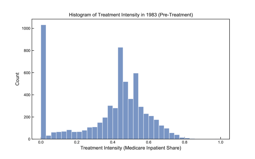
Figure 2: Histogram of treatment intensity (medicare share in 1983).

Figure 2 depicts the histogram of $D$ for 1983, which suggests that this treatment variable is suitable for our continuous DiD framework. Specifically, we note that a significant number of hospitals register at $D=0$, enabling us to consider these hospitals as the control group. Moreover, the positive Medicare shares ($D>0$) vary widely across hospitals and appear to follow a continuous distribution, which allows us to view these positive shares as continuous treatment intensities.

We now turn to the results for the repeated outcomes (panel) setting, where the outcome variable is the capital-labor ratio. In particular, using $t-1=1983$ as the pre-treatment year, we estimate the causal parameter ATT(d) at various intensities $d$ ranging from $0.1$ to $0.8$ for each $t=1984,1985,1986$. The results are shown in Figure 3.

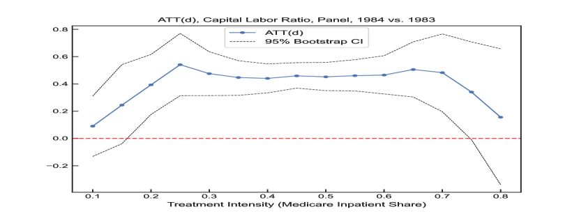
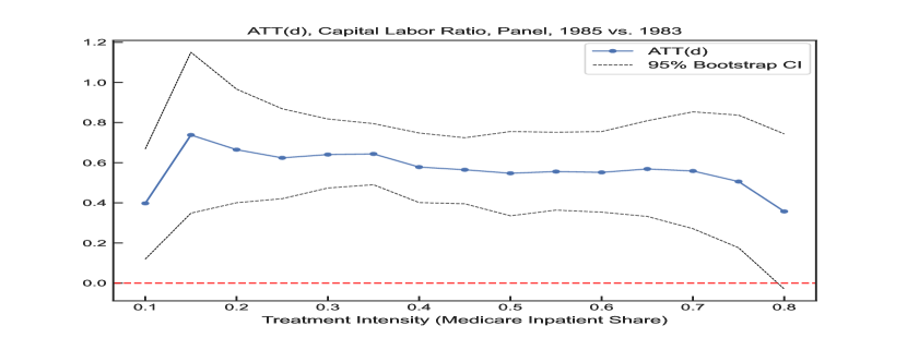
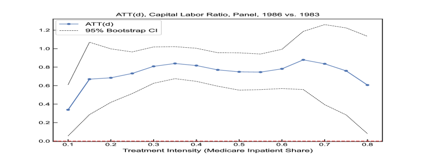
Figure 3: $\widehat{ATT}(d)$ for capital-labor ratio (panel data).

Specifically, we observe that all the estimated ATTs for the capital-labor ratio are positive, which corroborates the empirical findings in Acemoglu and Finkelstein (2008) and provides further evidence that the PPS reform led to an increase in the capital-labor ratio. Moreover, compared to the results from $t=1984$, the estimates for $t=1985$ and $t=1986$ are much larger in magnitude, which implies that the hospitals respond to the PPS reform gradually. For comparison, the estimated $\beta$ in Acemoglu and Finkelstein (2008) is $1.13$ for the capital-labor ratio, which is larger than all our estimates. Interestingly, the pattern of the increasing impact of the PPS reform by year is consistent with the alternative research specifications in Acemoglu and Finkelstein (2008) (see Table 2 column (3)).

Finally, for all three years, the estimated ATTs vary across treatment intensities and don’t display increasing trends, which is inconsistent with the theoretical prediction that hospitals with higher Medicare shares should experience a more substantial increase in the capital-labor ratio. In fact, our estimates indicate that the ATT increases with treatment intensity initially, but then decreases at higher levels of treatment intensity. One caveat is that the estimates are rather noisy at high treatment intensities where fewer observations are available.

Similarly, we present evidence of increased technological adoption following the PPS reform. The outcome variable here is the total number of various medical facilities in each hospital, which can be used as a measure of technological adoption. As with our prior analysis, we designate $t-1=1983$ as the pre-treatment year. However, due to data availability, we restrict our analysis of post-treatment years to $1984$ and $1985$. We then estimate the causal parameter ATT(d) at varying intensities $d$ ranging from $0.1$ to $0.8$ for both $t=1984$ and $t=1985$. The findings are shown in Figure 4.

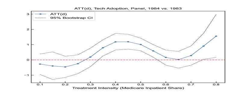
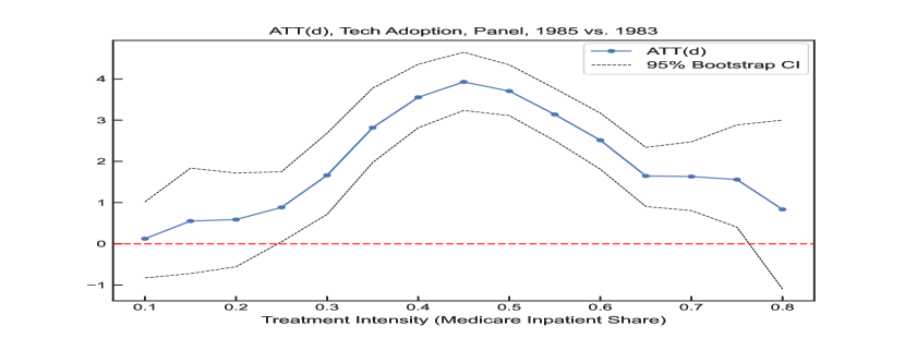
Figure 4: $\widehat{ATT}(d)$ for tech adoption (panel data).

Notably, the results shown in Figure 4 further reveal that the estimated ATTs for technological adoption are positive at all the treatment intensities we considered. This validates the theoretical prediction in Acemoglu and Finkelstein (2008) that the PPS reform should lead to an increase in technological adoption. Moreover, similar to the findings for the capital-labor ratio, the $1985$ estimates are much larger in magnitude compared to their $1984$ counterparts, further suggesting that the impact of the PPS reform is staggered over time. Finally, for both years, the estimates indicate a large degree of heterogeneity in the treatment effect across treatment intensities. Especially for $t=1985$, our estimates follow a clear hump-shaped pattern, increasing with treatment intensity initially but then decreasing at higher levels of treatment intensity. This pattern is again inconsistent with the theoretical prediction that hospitals with higher Medicare inpatient shares should experience a bigger increase in technological adoption following the PPS reform.

Since Acemoglu and Finkelstein (2008) use all the available data between 1980 and 1986 in their linear specification, we can alternatively apply our methods to averaged outcomes over all the available periods pre and post-treatment. The results are presented in Figure 5, which reinforces our previous findings that the treatment effect exhibits a large degree of heterogeneity across treatment intensities and there seems to be a hump-shaped pattern in the treatment curves.

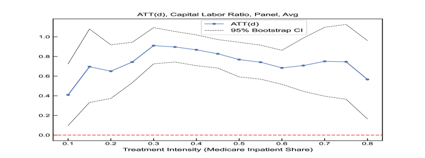
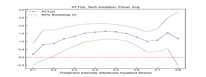
Figure 5: $\widehat{ATT}(d)$ average (panel data).

6.4 Results: repeated cross-sections setting

In our analysis thus far, we have closely followed the research design of Acemoglu and Finkelstein (2008), utilizing the Medicare share from 1983 as our quasi-experimental variation for causal analysis. However, it is crucial to acknowledge the potential changes in Medicare share as a result of the PPS reform. Specifically, the PPS reform could lead to a reduction in the Medicare share for hospitals with positive shares initially. Indeed, a comparison of the histograms of Medicare share between $1983$ and $1986$, as displayed in Figure 6, reveals a leftward shift in the distribution.

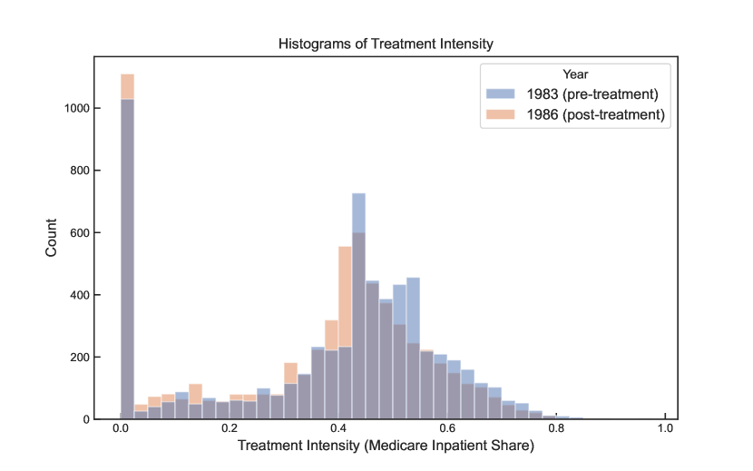
Figure 6: Histogram of treatment intensity (medicare share in 1983).

Therefore, to account for the changes in the treatment intensity (Medicare share) and covariates, we can alternatively treat the data as repeated cross-sections and apply our estimator accordingly. Specifically, we focus on the capital-labor ratio as our main outcome variable, and we estimate ATTs across a wide range of treatment intensities for $t-1=1983$ and $t=1984,1985,1986$. The results from our repeated cross-sections methods, as shown in Figure 7, differ considerably from those in the panel setting.

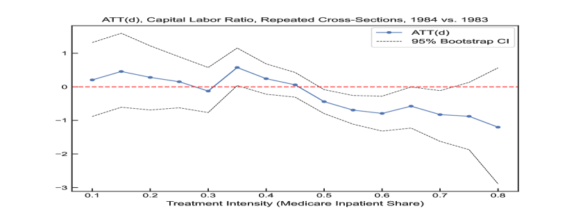
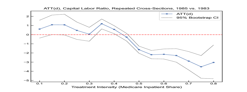
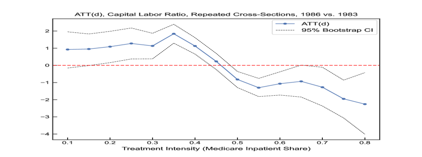
Figure 7: $\widehat{ATT}(d)$ for capital-labor ratio (repeated cross-sections).

Notably, most of the estimates for the year 1984 are not significantly different from zero. On the other hand, for the year 1985, the estimated ATTs are positive and large for low treatment intensities. However, as the treatment intensity increases, these estimates decrease in magnitude and can even become negative, and a similar trend holds for the year 1986 with larger estimates. This pattern markedly differs from what we see in the panel setting, where the estimated ATTs are consistently positive across all treatment intensities. These findings suggest that the PPS reform could lead to a decrease in the capital-labor ratio for hospitals with high Medicare inpatient shares, which is in contradiction to the theoretical predictions of Acemoglu and Finkelstein (2008). One possible explanation is that hospitals with a high volume of Medicare inpatients might have developed administrative and clinical systems to effectively manage these patients, making it easier to adapt to PPS changes. Nevertheless, further investigations and formal theoretical analysis are needed to understand the underlying mechanism behind this phenomenon.

Remark 6.4.

The estimates for the causal parameters are constructed based on the results from the previous section. Here are the details of our implementation. First, we employ a 5-fold cross-fitting with data randomly shuffled before the sample splitting step to avoid the clustering of data being over-represented in the subsamples. Moreover, we use the second-order Gaussian kernel with an undersmoothing bandwidth of $h=N^{-1/4}$ to estimate the density $f_{D}(d)$ and the conditional mean $E[K_{h}(D-d)|X]$. The infinite-dimensional nuisance parameters are estimated using Random Forest (RF). Specifically, we use the scikit-learn RF package from Python, with each estimate using 200 trees of maximum depth equal to 20. The main advantage of using RF is that it can handle both continuous and discrete covariates, which is crucial for our analysis since our covariates $X$ include both continuous variables and a large number of state dummies. However, we note that other ML methods, such as deep neural networks, can also be used to estimate the nuisance parameters. Moreover, the standard errors are calculated using the cross-fitted estimator defined in (4.3) and (4.4), and the 95-percent bootstrap confidence intervals shown in the figures were constructed using the multiplier bootstrap procedure defined in (4) and (4). For these bootstrap CIs, we use Gaussian multipliers $\{\xi_{i}\}_{i=1}^{N}$ drawn from a normal distribution with $E[\xi_{i}]=Var[\xi_{i}]=1$ for $B=1000$ repetitions.

7 Conclusion

This paper studies difference-in-differences models with continuous treatments. Our identification results are based on a conditional parallel trends assumption, allowing researchers to control for a rich set of covariates. Under the double/debiased machine learning framework, we develop estimators for the average treatment effect on the treated at each continuous treatment intensity and establish their asymptotic properties. Monte Carlo simulations demonstrate that our estimators perform well despite the highly non-linear relationship between the continuous treatment and the high-dimensional covariates. To illustrate the practical application of our methodologies, we revisit the research questions posed in Acemoglu and Finkelstein (2008), applying our estimators to their dataset and deriving new research insights. The extension of difference-in-differences models to the continuous treatment setting has important implications for empirical research. Our methods provide researchers with new tools for examining the impacts of continuous treatment variables.

8 Appendix A: Monte Carlo Simulation

Data-generating process, repeated outcomes setting: (a) $p=100$ dimensional covariates $X\sim N(0,\Sigma)$, where the covariance matrix $\Sigma$ has variances equal to $1$ on the diagonal and covariances equal to $0.1$ on the off-diagonal; (b) the propensity score for the control group is generated according to $P(D=0|X)=1/(1+\exp(-X^{\prime}\gamma))$, with $\gamma_{j}=0.5j^{-2}$; (c) for the treatment group $D>0$, the continuous treatment is generated according to $D|X,V\sim\text{Exp}(|X^{\prime}\alpha+V|)$, where $V\perp X$, $V\sim N(0,1)$, $\alpha_{j}=0.3j^{-2}$; (d) the potential outcomes are generated according to $Y_{t-1}(0)=\epsilon_{1}$, $Y_{t}(0)=Y_{t-1}(0)+X^{\prime}\beta+1+\epsilon_{2}$, $Y_{t}(D)=Y_{t}(0)-0.5D^{2}+\epsilon_{3}$, where $\beta_{j}=0.5/j$ for $j=1,\cdots,6$ and $0$ otherwise, and all the errors $\epsilon_{1},\epsilon_{2},\epsilon_{3}$ have independent standard normal distributions. The observed data are $(Y_{i,t-1},Y_{i,t},X_{i},D_{i})$, with $Y_{t-1}=Y_{t-1}(0)$ and $Y_{t}=1{D>0}Y_{t}(D)+1{D=0}Y_{t}(0)$.

Data-generating process, repeated cross-sections setting: (a) time indicator $T$ is generated according to $T\sim\text{Bernoulli}(0.5)$; (b) $p=100$ dimensional variable $Z\sim N(0,\Sigma)$, where the covariance matrix $\Sigma$ has variances equal to $1$ on the diagonal and covariances equal to $0.1$ on the off-diagonal; (c) the time-varying covariates $X$ are generated through $X=Z+0.3(T\times V)$ where $V$ is a $p$-dimensional normal distribution with an identity covariance matrix; (d) the propensity score for the control group is generated according to $P(D=0|X)=1/(1+\exp(-X^{\prime}\gamma))$, with $\gamma_{j}=0.5j^{-2}$; (e) for the treatment group $D>0$, the continuous treatment is generated according to $D|X,V\sim\text{Exp}(|X^{\prime}\alpha+U|)$, where $U\perp X$, $U\sim N(0,1)$, $\alpha_{j}=0.3j^{-2}$; (f) the potential outcomes are generated according to $Y_{t-1}(0)=\epsilon_{1}$, $Y_{t}(0)=Y_{t-1}(0)+X^{\prime}\beta+1+\epsilon_{2}$, $Y_{t}(D)=Y_{t}(0)-0.5D^{2}+\epsilon_{3}$, where $\beta_{j}=0.5/j$ for $j=1,\cdots,6$ and $0$ otherwise, and all the errors $\epsilon_{1},\epsilon_{2},\epsilon_{3}$ have independent standard normal distributions. The observed data are $(Y_{i},T_{i},X_{i},D_{i})$, with $Y=TY_{t}+(1-T)Y_{t-1}$, $Y_{t-1}=Y_{t-1}(0)$, $Y_{t}=1{D>0}Y_{t}(D)+1{D=0}Y_{t}(0)$.

In our simulations, the propensity score for the control group $P(D=0|X)$ is estimated using a 5-fold cross-validated Logit LASSO. The conditional density $f_{h}(d|X)=E[K_{h}(D-d)|X]$ is estimated nonparametrically using random forests with 100 trees, each of maximum depth 10. The term $E[Y_{t}-Y_{t-1}|X,D=0]$ is estimated using a 5-fold cross-validated LASSO. We also use an undersmoothing kernel bandwidth $h=0.5N^{-4}$ throughout our simulations. We consider sample sizes $N=2000$ and $10000$ for both repeated outcomes and repeated cross-sections cases, and we conduct $B=500$ simulations in each setting.

The DGP implies the true $ATT(d)=-0.5d^{2}$, and we focus on a specific treatment intensity $d=0.9$. The histograms of these simulation estimates are shown in Figure 8, where the red lines indicate the true ATT. We see that as the sample size increases, both the bias and variance decrease. The simulation estimates seem to follow a normal distribution in each case, which is consistent with our asymptotic theory.

Figure 8: The simulation results, true $ATT(d)=0.405$.

Table 1: Monte Carlo simulation results.

Method and Sample Size	Bias	Std	RMSE	AVSE	Coverage
panel, n=2000	0.0247	0.0994	0.1024	0.0999	0.9440
panel, n=10000	0.0132	0.0548	0.0563	0.0550	0.9360
cross-sections, n = 2000	0.0093	0.2553	0.2555	0.2620	0.9520
cross-sections, n = 10000	-0.0027	0.1459	0.1460	0.1441	0.9500

In Table 1, we report the bias, standard deviation of estimated ATTs (Std), root-mean-squared error (RMSE), average standard deviations (AVSE), and coverage probability of 95 percent confidence intervals. In both settings, the bias, standard deviation, and RMSE decrease as the sample size increases. The standard deviations of simulation estimates are very close to the average estimated standard errors, which suggests that our variance estimators perform well. The coverage of the estimated confidence intervals is close to 95 percent, although there seems to be a slight undercoverage in the panel setting.

These simulation results demonstrate that our estimators perform well. We designed sophisticated DGPs so that the relationship between the continuous treatment variable and high-dimensional covariates was highly non-linear. Moreover, although the 100-dimensional covariates were generated from normal distributions, we intentionally specified the covariance matrix so that these variables were correlated with each other. Notably, the conditional density with 100 covariates was estimated nonparametrically using our proposed methods despite the relatively small sample size. The undersmoothing kernel bandwidth seems to work as predicted by the theory to reduce the asymptotic bias. Due to computational concerns, we were unable to use more sophisticated machine learners in our simulations. Therefore, we expect the performance of our estimators to improve further if such machine learners are employed.

9 Appendix B: Proofs of results

Proof of Theorem 2.1: By definition, $ATT(d)=E[Y_{t}(d)-Y_{t}(0)|D=d]$. First,

$$E[Y_{t}-Y_{t-1}|D=d]=E[Y_{t}(d)-Y_{t-1}(0)|D=d]$$ (9.2)

by the fact that $Y_{t}=Y_{t}(D)$ and $Y_{t-1}=Y_{t-1}(0)$.

Second,

$$E\bigg{[}(Y_{t}-Y_{t-1})\mathbf{1}\{D=0\}\frac{f_{D|X}(d)}{f_{D}(d)P(D=0|X)}\bigg{]}$$

$$=E\bigg{[}(Y_{t}-Y_{t-1})\frac{f_{D|X}(d)}{f_{D}(d)P(D=0|X)}|D=0\bigg{]}P(D=0)$$

$$=\int E[(Y_{t}(0)-Y_{t-1}(0))|X=x,D=0]\frac{f_{D|X}(d|x)P(D=0)}{f_{D}(d)P(D=0|X=x)}f_{X|D=0}(x)dx$$

$$=\int E[(Y_{t}(0)-Y_{t-1}(0))|X=x,D=d]$$

$$\times\frac{f_{D|X=x}(d)P(D=0)}{f_{D}(d)P(D=0|X=x)}\frac{P(D=0|X=x)f_{X}(x)}{P(D=0)}dx$$

$$=\int E[(Y_{t}(0)-Y_{t-1}(0))|X=x,D=d]f_{X|D=d}(x)dx$$

$$=E[(Y_{t}(0)-Y_{t-1}(0))|D=d]$$ (9.3)

where the first equality holds by the law of total probability, the second equality holds by the law of iterated expectation, the third equality holds by that $Y_{t}=Y_{t}(D)$ and $Y_{t-1}=Y_{t-1}(0)$, the fourth equality holds by Bayes’ rule and conditional parallel trend, and the fifth equality holds by the law of iterated expectation.

Then combining the above results, we have

$$E[Y_{t}-Y_{t-1}|D=d]-E\bigg{[}(Y_{t}-Y_{t-1})\mathbf{1}\{D=1\}\frac{f_{D|X}(d)}{f_{D}(d)P(D=0|X)}\bigg{]}$$

$$=E[Y_{t}(d)-Y_{t-1}(0)|D=d]-E[Y_{t}(0)-Y_{t-1}(0)|D=d]$$

$$=E[Y_{t}(d)-Y_{t}(0)|D=d]$$

$$=ATT(d)$$ (9.4)

Next, for repeated cross-sections, we have

$$E\bigg{[}\frac{T-\lambda}{\lambda(1-\lambda)}Y|D=d\bigg{]}$$

$$=E\bigg{[}E\bigg{[}\frac{T-\lambda}{\lambda(1-\lambda)}Y|D=d,T\bigg{]}|D=d\bigg{]}$$

$$=E\bigg{[}\frac{T-\lambda}{\lambda(1-\lambda)}Y|D=d,T=1\bigg{]}P(T=1|D=d)$$

$$+E\bigg{[}\frac{T-\lambda}{\lambda(1-\lambda)}Y|D=d,T=0\bigg{]}P(T=0|D=d)$$

$$=E\bigg{[}\frac{1-\lambda}{\lambda(1-\lambda)}Y|D=d,T=1\bigg{]}\lambda+E\bigg{[}\frac{0-\lambda}{\lambda(1-\lambda)}Y|D=d,T=0\bigg{]}(1-\lambda)$$

$$=E[Y_{t}|D=d]-E[Y_{t-1}|D=d]$$

$$=E[Y_{t}-Y_{t-1}|D=d]$$ (9.5)

where the first equality holds by law of iterated expectation, the second equality holds by definition, and the last two equalities hold by Assumption 2.2. $\square$

Proof of Lemma 3.1: First, consider the repeated outcomes case. Define the unadjusted score $\varphi_{h}$ as

$$\varphi_{h}:=\Delta Y\frac{K_{h}(D-d)g_{0}(X)-\mathbf{1}\{D=0\}f_{h}^{0}(d|X)}{f_{d}^{0}g_{0}(X)}-ATT_{h}(d)$$ (9.6)

where we use the following notation: $\Delta Y=Y_{t}-Y_{t-1}$, $f_{d}^{0}:=f_{D}(d)$, $f_{h}^{0}(d|X):=E[K_{h}(D-d)|X]$, $g_{0}(X):=P(D=0|X)$. We will add an adjustment term to the original score so that the new score satisfies the Neyman orthogonality w.r.t. the infinite-dimensional parameters.

The two infinite-dimensional nuisance parameters are $f_{h}^{0}(d|X)$ and $g_{0}(X)$, and in particular, they satisfy $f_{h}^{0}(d|X)=E[K_{h}(D-d)|X]$ and $g_{0}(X)=E[\mathbf{1}\{D=0\}|X]$. Then the adjustment term $c_{h}$ takes the form

$$c_{h}:=(K_{h}(D-d)-f_{h}^{0}(d|X))E[\partial_{1}\varphi_{h}|X]+(\mathbf{1}\{D=0\}-g_{0}(X))E[\partial_{2}\varphi_{h}|X]$$ (9.7)

where $\partial_{1}$ and $\partial_{2}$ denote the partial derivatives with respect to $f_{h}^{0}(d|X)$ and $g_{0}(X)$ respectively. Then, we have

$$c_{h} =(\mathbf{1}\{D=0\}-g_{0}(X))\frac{f_{h}^{0}(d|X)}{f_{d}^{0}\cdot g_{0}^{2}(X)}E[\Delta Y\mathbf{1}\{D=0\}|X]$$

$$-(K_{h}(D-d)-f_{h}^{0}(d|X))\frac{1}{f_{d}^{0}\cdot g_{0}(X)}E[\Delta Y\mathbf{1}\{D=0\}|X]$$

$$=\frac{[\mathbf{1}\{D=0\}-g_{0}(X)]f_{h}^{0}(d|X)-[K_{h}(D-d)-f_{h}^{0}(d|X)]g_{0}(X)}{f_{d}^{0}\cdot g_{0}(X)}\underbrace{\frac{E[\Delta Y\mathbf{1}\{D=0\}|X]}{g_{0}(X)}}_{:=\mathcal{E}_{\Delta Y}^{0}(X)}$$

$$=\frac{\mathbf{1}\{D=0\}f_{h}^{0}(d|X)-K_{h}(D-d)g_{0}(X)}{f_{d}^{0}\cdot g_{0}(X)}\mathcal{E}_{\Delta Y}^{0}(X)$$ (9.8)

where $\mathcal{E}_{\Delta Y}^{0}(X)=E[\Delta Y\mathbf{1}\{D=0\}|X]/g_{0}(X)=E[\Delta Y|D=0,X]$. In particular, note that $\psi_{h}$ in the lemma satisfies $\psi_{h}=\varphi_{h}+c_{h}$.

Now it remains to show the new score $\psi_{h}$ satisfies Neyman orthogonality w.r.t. the nuisance parameters, $f_{h}^{0}(d|X)$, $g_{0}(X)$, and $\mathcal{E}_{\Delta Y}^{0}(X)$. First, we need to check the moment condition $E[\psi_{h}]=0$. Since $E[\varphi_{h}]=0$, we only need to check $E[c_{h}]=0$:

$$E[c_{h}] =E\bigg{[}\frac{\mathbf{1}\{D=0\}f_{h}^{0}(d|X)-K_{h}(D-d)g_{0}(X)}{f_{d}^{0}\cdot g_{0}(X)}\mathcal{E}_{\Delta Y}^{0}(X)\bigg{]}$$

$$=E\bigg{[}\frac{E[\mathbf{1}\{D=0\}|X]f_{h}^{0}(d|X)-E[K_{h}(D-d)|X]g_{0}(X)}{f_{d}^{0}\cdot g_{0}(X)}\mathcal{E}_{\Delta Y}^{0}(X)\bigg{]}$$

$$=E\bigg{[}\frac{g_{0}(X)f_{h}^{0}(d|X)-f_{h}^{0}(d|X)g_{0}(X)}{f_{d}^{0}\cdot g_{0}(X)}\mathcal{E}_{\Delta Y}^{0}(X)\bigg{]}$$

$$=0$$ (9.9)

where the second equality holds by the law of iterated expectation and the third equality holds by the fact that $E[K_{h}(D-d)|X]=f_{h}^{0}(d|X)$ and $E[\mathbf{1}\{D=0\}|X]=g_{0}(X)$.

Second, we need to show the Gateaux derivative of the score w.r.t. the nuisance parameters $\eta_{0}:=(f_{h}^{0}(d|X),g_{0}(X),\mathcal{E}_{\Delta Y}^{0}(X))$ vanishes at zero, that is, we need to show

$$\partial_{r}E[\psi_{h}(\eta_{0}+r(\eta-\eta_{0}))]|_{r=0}=0.$$ (9.10)

We use the notation $\eta$ without the subscript $0$ to denote generic nuisance parameters in the set $\mathcal{T}_{n}$. By the definition of Gateaux derivative, it suffices to show the partial derivative is zero w.r.t. each nuisance parameter separately. In particular, in the following derivations, by assumption in the lemma, we can use the dominated convergence theorem to interchange the derivatives and the expectations.

w.r.t $f_{h}(d|X)$:

$$\partial_{r}E[\psi_{h}(f_{h}^{0}(d|X)+r(f_{h}(d|X)-f_{h}^{0}(d|X)))]|_{r=0}$$

$$=E\bigg{[}\frac{\mathbf{1}\{D=0\}\Delta f_{h}(d|X)}{f_{d}^{0}\cdot g_{0}(X)}(\Delta Y-\mathcal{E}_{\Delta Y}^{0}(X))\bigg{]}$$

$$=E\bigg{[}\frac{E[\mathbf{1}\{D=0\}\Delta Y|X]}{g_{0}(X)}\frac{\Delta f_{h}(d|X)}{f_{d}^{0}}-\frac{E[\mathbf{1}\{D=0\}|X]}{g_{0}(X)}\frac{\Delta f_{h}(d|X)}{f_{d}^{0}}\mathcal{E}_{\Delta Y}^{0}(X)\bigg{]}$$

$$=E\bigg{[}\mathcal{E}_{\Delta Y}^{0}(X)\frac{\Delta f_{h}(d|X)}{f_{d}^{0}}-\frac{g_{0}(X)}{g_{0}(X)}\frac{\Delta f_{h}(d|X)}{f_{d}^{0}}\mathcal{E}_{\Delta Y}^{0}(X)\bigg{]}$$

$$=0$$ (9.11)

where the first equality holds by definition with $\Delta f_{h}(d|X):=f_{h}(d|X)-f_{h}^{0}(d|X)$, the second equality holds by the law of iterated expectation, and the third equality holds by the fact that $E[\Delta Y\mathbf{1}\{D=0\}|X]/g_{0}(X)=\mathcal{E}_{\Delta Y}^{0}(X)$ and $E[\mathbf{1}\{D=0\}|X]=g_{0}(X)$.

w.r.t $g(X)$:

$$\partial_{r}E[\psi_{h}(g_{0}(X)+r(g(X)-g_{0}(X)))]|_{r=0}$$

$$=E\bigg{[}-\frac{\mathbf{1}\{D=0\}f_{h}^{0}(d|X)}{f_{d}^{0}\cdot g_{0}^{2}(X)}(\Delta Y-\mathcal{E}_{\Delta Y}^{0}(X))\Delta g(X)\bigg{]}$$

$$=E\bigg{[}-\Delta g(X)\frac{E[\mathbf{1}\{D=0\}\Delta Y|X]}{g_{0}(X)}\frac{f_{h}^{0}(d|X)}{f_{d}^{0}g_{0}(X)}+\Delta g(X)\frac{E[\mathbf{1}\{D=0\}|X]}{g_{0}(X)^{2}}\frac{f_{h}^{0}(d|X)}{f_{d}^{0}}\mathcal{E}_{\Delta Y}^{0}(X)\bigg{]}$$

$$=E\bigg{[}-\Delta g(X)\mathcal{E}_{\Delta Y}^{0}(X)\frac{f_{h}^{0}(d|X)}{f_{d}^{0}g_{0}(X)}+\Delta g(X)\frac{g_{0}(X)}{g_{0}(X)^{2}}\frac{f_{h}^{0}(d|X)}{f_{d}^{0}}\mathcal{E}_{\Delta Y}^{0}(X)\bigg{]}$$

$$=0$$ (9.12)

where the first equality holds by chain rule and the definition $\Delta g(X):=g(X)-g_{0}(X)$, second equality holds by law of iterated expectation, and the third equality holds by that $E[\Delta Y\mathbf{1}\{D=0\}|X]/g_{0}(X)=\mathcal{E}_{\Delta Y}^{0}(X)$ and $E[\mathbf{1}\{D=0\}|X]=g_{0}(X)$.

w.r.t $\mathcal{E}_{\Delta Y}(X)$:

$$\partial_{r}E[\psi_{h}(\mathcal{E}_{\Delta Y}^{0}(X)+r(\mathcal{E}_{\Delta Y}(X)-\mathcal{E}_{\Delta Y}^{0}(X)))]|_{r=0}$$

$$=E[\frac{K_{h}(D-d)g_{0}(X)-\mathbf{1}\{D=0\}f_{h}^{0}(d|X)}{f_{d}^{0}\cdot g_{0}(X)}\Delta\mathcal{E}(X)]$$

$$=E[\frac{E[K_{h}(D-d)|X]g_{0}(X)-E[\mathbf{1}\{D=0\}|X]f_{h}^{0}(d|X)}{f_{d}^{0}\cdot g_{0}(X)}\Delta\mathcal{E}(X)]$$

$$=0$$ (9.13)

where the first line holds by definition with $\Delta\mathcal{E}(X)=\mathcal{E}_{\Delta Y}(X)-\mathcal{E}_{\Delta Y}^{0}(X)$, the second equality holds by law of iterated expectation, and the last equality holds by the definition that $E[K_{h}(D-d)|X]=f_{h}^{0}(d|X)$ and $E[\mathbf{1}\{D=0\}|X]=g_{0}(X)$.

This shows that the score $\psi_{h}$ is Neyman orthogonal w.r.t. the infinite-dimensional nuisance parameters. The proof for the repeated cross-sections case follows the same argument by replacing $\Delta Y$ with $\frac{T-\lambda}{\lambda(1-\lambda)}Y$. $\square$

Proof of Lemma 4.2: We focus on the repeated outcomes case. The bias $B_{h}(d)$ is defined as

$$B_{h}(d):= ATT(d)-ATT_{h}(d)$$

$$= E[\Delta Y|D=d]-E\bigg{[}\Delta Y\mathbf{1}\{D=0\}\frac{f_{D|X}(d|X)}{f_{D}(d)P(D=0|X)}\bigg{]}$$

$$- E\bigg{[}\Delta Y\frac{K_{h}(D-d)P(D=0|X)-\mathbf{1}\{D=0\}E[K_{h}(D-d)|X]}{f_{D}(d)P(D=0|X)}\bigg{]}$$

$$= \bigg{(}E[\Delta Y|D=d]-E\bigg{[}\Delta Y\frac{K_{h}(D-d)}{f_{D}(d)}\bigg{]}\bigg{)}$$

$$- E\bigg{[}\Delta Y\mathbf{1}\{D=0\}\frac{f_{D|X}(d|X)-E[K_{h}(D-d)|X]}{f_{D}(d)P(D=0|X)}\bigg{]}.$$ (9.14)

First, note that

$$E[\Delta Y|D=d]-E\bigg{[}\Delta Y\frac{K_{h}(D-d)}{f_{D}(d)}\bigg{]}$$

$$= \int t\frac{f_{\Delta Y,D}(t,d)}{f_{D}(d)}dt-\int t\frac{1}{f_{D}(d)}\int\frac{1}{h}K\Big{(}\frac{s-d}{h}\Big{)}f_{\Delta Y,D}(t,s)dsdt$$

$$= \int C_{1}\frac{t}{f_{D}(d)}h^{2}f_{\Delta Y,D}^{(2)}(t,d)dt+o(h^{2})$$

$$= O(h^{2})$$ (9.15)

where the first equality holds by definition, the second equality holds by change of variables and Taylor expansion (see Lemma 5.1 in Fan and Yao (2003)), and the last equality holds by assumption.

Second, by the same argument using the change of variables and Taylor expansion, we have

$$E[K_{h}(D-d)|X=x] =\int\frac{1}{h}K\Big{(}\frac{d-s}{h}\Big{)}f_{D|X}(s|x)ds$$

$$=\int K(u)f_{D|X}(d+hu|x)du$$

$$=f_{D|X}(d|x)+C_{2}h^{2}f_{D|X}^{(2)}(d|x)+o(h^{2}).$$ (9.16)

Then by the uniform boundedness of $f^{(2)}_{D|X}(d|x)$ and assumptions on $\Delta Y,f_{D}(d),P(D=0|X)$, applying the dominated convergence theorem, we have

$$E\bigg{[}\Delta Y\mathbf{1}\{D=0\}\frac{f_{D|X}(d|X)-E[K_{h}(D-d)|X]}{f_{D}(d)P(D=0|X)}\bigg{]}$$ (9.17)

$$= C_{3}h^{2}E\bigg{[}\Delta Y\mathbf{1}\{D=0\}\frac{f_{D|X}^{(2)}(d|X)}{f_{D}(d)P(D=0|X)}\bigg{]}+o(h^{2})$$ (9.18)

$$= O(h^{2}).$$ (9.19)

Combining the two results, we have $B_{h}(d)=O(h^{2})$, which completes the proof. The proof for the repeated cross-sections case follows the same argument by replacing $\Delta Y$ with $\frac{T-\lambda}{\lambda(1-\lambda)}Y$. $\square$

Proof of Theorem 4.2 (Repeated Outcomes): Let $T_{N}$ be the set of square integrable nuisance parameters $\eta:=(f_{h}(d|X),g(X),\mathcal{E}_{\Delta Y}(X))$ such that assumption 4.7 holds. Let $F_{N}$ be the set of $f>0$ such that $|f-f_{d}^{0}|\leq(Nh)^{-1/2}$. Then assumption 4.7 implies that, with probability tending to 1, $\hat{\eta}_{k}\in T_{N}$ and $\hat{f}_{d,k}\in F_{N}$. Throughout the proof, we use $N$ to denote the sample size and $n:=N/K$ to denote the size of any of the subsamples. In particular, since $K$ is fixed, $n\asymp N$.

To simplify notation, let $\theta_{0}$ denote the true $ATT(d)$, $\theta_{0h}$ denote the true $ATT_{h}(d)$, and $\hat{\theta}_{h}$ denote our cross-fitted estimator. In particular, recall that our estimator is

$$\hat{\theta}_{h} :=\frac{1}{K}\sum_{k=1}^{K}\frac{1}{n}\sum_{i\in I_{k}}\frac{K_{h}(D_{i}-d)\hat{g}_{k}(X_{i})-\mathbf{1}\{D_{i}=0\}\hat{f}_{h,k}(d|X_{i})}{\hat{f}_{d,k}\hat{g}_{k}(X_{i})}\big{(}\Delta Y_{i}-\hat{\mathcal{E}}_{\Delta Y,k}(X_{i})\big{)}.$$ (9.20)

Then we can decompose the following difference as

$$\hat{\theta}_{h}-\theta_{0}=\underbrace{\hat{\theta}_{h}-\theta_{0h}}_{(1)}+\underbrace{\theta_{0h}-\theta_{0}}_{(2)}$$ (9.21)

where $(1)$ will be our main focus while the bias term $(2)$ is shown in Lemma 4.2 to be $O(h^{2})$ and asymptotically negligible by the assumption of the under-smoothing bandwidth.

By definition,

$$\sqrt{N}(\hat{\theta}_{h}-\theta_{0h})=\sqrt{N}\frac{1}{K}\sum_{k=1}^{K}E_{n,k}[\psi_{h}(Z_{i},\theta_{0,h},\hat{f}_{d,k},\hat{\eta}_{k})]$$ (9.22)

where $\psi_{h}$ is defined as in (3.8), and $E_{n,k}(f)=\frac{1}{n}\sum_{i\in I_{k}}f(Z_{i})$ denotes the empirical average of a generic function $f$ over the set $I_{k}$. Then we have the following decomposition, using Taylor’s theorem:

$$\sqrt{N}(\hat{\theta}_{h}-\theta_{0h}) =\sqrt{N}\frac{1}{K}\sum_{k=1}^{K}E_{n,k}[\psi_{h}(Z,\theta_{0h},f_{d}^{0},\hat{\eta}_{k})]$$ (9.23)

$$+\sqrt{N}\frac{1}{K}\sum_{k=1}^{K}E_{n,k}[\partial_{f}\psi_{h}(Z,\theta_{0h},f_{d}^{0},\hat{\eta}_{k})](\hat{f}_{d,k}-f_{d}^{0})$$ (9.24)

$$+\sqrt{N}\frac{1}{K}\sum_{k=1}^{K}E_{n,k}[\partial_{f}^{2}\psi_{h}(Z,\theta_{0h},\bar{f}_{k},\hat{\eta}_{k})](\hat{f}_{d,k}-f_{d}^{0})^{2}$$ (9.25)

where $\bar{f}_{k}\in(f_{d}^{0},\hat{f}_{d,k})$. This decomposition provides a roadmap for the remainder of the proof. There are roughly four steps. In the first step, we show the second-order term (9.25) vanishes rapidly and does not contribute to the asymptotic variance. In the second step, we bound the first-order term (9.24), which potentially contributes to the asymptotic variance. In step 3, we expand (9.23) around the nuisance parameter $\hat{\eta}_{k}$, in which the first-order bias disappears by Neyman orthogonality, and we show the second-order terms have no impact on the asymptotics under our assumptions. In the final step, we verify the results used in the first two steps and conclude.

Before we start the main proof, we state two well-known results that will be used in the proof. For an i.i.d. sample $\{D_{i}\}_{i=1}^{n}$, the kernel estimator for the density $f_{D}(d):=f_{d}^{0}$ in our setting is defined as

$$\hat{f}_{d}:=\frac{1}{n}\sum_{i=1}^{n}K_{h}(D_{i}-d).$$ (9.26)

Then,

$$\hat{f}_{d}-f_{d}^{0}=\hat{f}_{d}-E[K_{h}(D-d)]-(f_{d}^{0}-E[K_{h}(D-d)]).$$ (9.27)

One can show that (see for example, Härdle (1990))

$$\hat{f}_{d}-E[K_{h}(D-d)] =O_{p}((nh)^{-1/2})$$ (9.28)

$$f_{d}^{0}-E[K_{h}(D-d)] =O(h^{2}).$$ (9.29)

Therefore, for an under-smoothing $h=o(n^{-1/5})$, we have $\hat{f}_{d}-f_{d}^{0}=O_{p}((nh)^{-1/2})$ and $(\hat{f}_{d}-f_{d}^{0})^{2}=O_{p}((nh)^{-1})$.

Step 1: Second Order Terms

First, we consider (9.25). By triangle inequality, we have

$$|E_{n,k}[\partial_{f}^{2}\psi_{h}(Z,\theta_{0h},\bar{f}_{k},\hat{\eta}_{k})]-E[\partial_{f}^{2}\psi_{h}(Z,\theta_{0h},f_{d}^{0},\eta_{0})]|$$

$$\leq \underbrace{|E_{n,k}[\partial_{f}^{2}\psi_{h}(Z,\theta_{0h},\bar{f}_{k},\hat{\eta}_{k})]-E_{n,k}[\partial_{f}^{2}\psi_{h}(Z,\theta_{0h},f_{d}^{0},\eta_{0})]|}_{J_{1k}}$$

$$+ \underbrace{|E_{n,k}[\partial_{f}^{2}\psi_{h}(Z,\theta_{0h},f_{d}^{0},\eta_{0})]-E[\partial_{f}^{2}\psi_{h}(Z,\theta_{0h},f_{d}^{0},\eta_{0})]|}_{J_{2k}}.$$

To bound $J_{2k}$, note that since $f_{d}^{0}$ is bounded away from zero and the score $\psi$ is bounded by $M_{h}$,

$$\partial_{f}^{2}\psi_{h}(Z,\theta_{0h},f_{d}^{0},\eta_{0})=\frac{2}{(f_{d}^{0})^{2}}(\psi_{h}(Z,\theta_{0h},f_{d}^{0},\eta_{0})+\theta_{0h})$$ (9.30)

which implies that

$$E[J_{2k}^{2}] =E\bigg{[}\bigg{(}\frac{1}{n}\sum_{i\in I_{k}}\partial_{f}^{2}\psi_{h}(Z,\theta_{0J},f_{d}^{0},\eta_{0})-E[\partial_{f}^{2}\psi_{h}(Z,\theta_{0h},f_{d}^{0},\eta_{0})]\bigg{)}^{2}\bigg{]}$$

$$=E\bigg{[}\bigg{(}\frac{1}{n}\sum_{i\in I_{k}}\partial_{f}^{2}\psi_{h}(Z,\theta_{0h},f_{d}^{0},\eta_{0})\bigg{)}^{2}\bigg{]}-\big{(}E[\partial_{f}^{2}\psi_{h}(Z,\theta_{0h},f_{d}^{0},\eta_{0})]\big{)}^{2}$$

$$\leq\frac{1}{n}E[(\partial_{f}^{2}\psi_{h}(Z,\theta_{0h},f_{d}^{0},\eta_{0}))^{2}]$$

$$\lesssim E[K_{h}^{2}(D-d)]/N$$

$$\lesssim(hN)^{-1},$$ (9.31)

where the third line holds by Cauchy-Schwarz inequality and Jensen’s inequality, the fourth line holds by the boundedness assumption on the components of the score, and the last line holds by the assumption on the kernel function $K$. Then by the Markov’s inequality, we have $J_{2k}\leq O_{p}\big{(}(Nh)^{-1/2}\big{)}$.

Next, for $J_{1k}$, we have

$$E[J_{1k}^{2}|I_{k}^{c}] =E[|E_{n,k}[\partial_{f}^{2}\psi_{h}(Z,\theta_{0h},\bar{f}_{k},\hat{\eta}_{k})]-E_{n,k}[\partial_{f}^{2}\psi_{h}(Z,\theta_{0h},f_{d}^{0},\eta_{0})]|^{2}|I_{k}^{c}]$$

$$\leq\sup_{f\in F_{N},\eta\in T_{N}}E[|\partial_{f}^{2}\psi_{h}(Z,\theta_{0h},f,\eta)-\partial_{f}^{2}\psi_{h}(Z,\theta_{0h},f_{d}^{0},\eta_{0})|^{2}|I_{k}^{c}]$$

$$\leq\sup_{f\in F_{N},\eta\in T_{N}}E[|\partial_{f}^{2}\psi_{h}(Z,\theta_{0h},f,\eta)-\partial_{f}^{2}\psi_{h}(Z,\theta_{0h},f_{d}^{0},\eta_{0})|^{2}]$$

$$\lesssim h^{-1}\varepsilon_{N}^{2},\quad\quad\quad\text{(a)}$$

where the second line holds by Cauchy-Schwarz inequality and the definition of supremum over the sets $F_{N}$ and $T_{N}$, and the third line holds since the supremum does not depend on the sample $I_{k}^{c}$. Then by conditional Markov’s inequality, $J_{1k}\leq O_{p}(h^{-1/2}\varepsilon_{N})$. Using the previous result that $(\hat{f}_{d,k}-f_{d}^{0})^{2}=O_{p}((Nh)^{-1})$, we conclude that (9.25) = $o_{p}(1)$. We will verify (a) at the end of this section.

Step 2: First-Order Terms

To bound (9.24), we first use the triangle inequality to obtain the decomposition

$$|E_{n,k}[\partial_{f}\psi_{h}(Z,\theta_{0h},f_{d}^{0},\hat{\eta}_{k})]-E[\partial_{f}\psi_{h}(Z,\theta_{0h},f_{d}^{0},\eta_{0})]|$$

$$\leq \underbrace{|E_{n,k}[\partial_{f}\psi_{h}(Z,\theta_{0h},f_{d}^{0},\hat{\eta}_{k})]-E_{n,k}[\partial_{f}\psi_{h}(Z,\theta_{0h},f_{d}^{0},\eta_{0})]|}_{J_{3k}}$$

$$+ \underbrace{|E_{n,k}[\partial_{f}\psi_{h}(Z,\theta_{0h},f_{d}^{0},\eta_{0})]-E[\partial_{f}\psi_{h}(Z,\theta_{0h},f_{d}^{0},\eta_{0})]|}_{J_{4k}}.$$

We first bound $J_{4k}$: By definition, we have

$$\partial_{f}\psi_{h}(Z,\theta_{0h},f_{d}^{0},\eta_{0})=-\frac{1}{f_{d}^{0}}(\psi_{h}(Z,\theta_{0h},f_{d}^{0},\eta_{0})+\theta_{0h}).$$ (9.32)

By the boundedness assumption,

$$E[J_{4k}^{2}]\leq\frac{1}{N}E[(\partial_{f}\psi_{h}(Z,\theta_{0h},f_{d}^{0},\eta_{0}))^{2}]\lesssim(Nh)^{-1}.$$ (9.33)

Then by Markov’s inequality, we have $J_{4k}\leq O_{p}((Nh)^{-1/2})$. With the assumption that $Nh\to\infty$, we have $J_{4k}=o_{p}(1)$.

Second, to bound $J_{3k}$, note that

$$E[J_{3k}^{2}|I_{k}^{c}] =E[|E_{n,k}[\partial_{f}\psi_{h}(Z,\theta_{0h},f_{d}^{0},\hat{\eta}_{k})]-E_{n,k}[\partial_{f}\psi_{h}(Z,\theta_{0h},f_{d}^{0},\eta_{0})]|^{2}|I_{k}^{c}]$$

$$\leq\sup_{\eta\in T_{N}}E[|\partial_{f}\psi_{h}(Z,\theta_{0h},f_{d}^{0},\eta)-\partial_{f}\psi_{h}(Z,\theta_{0h},f_{d}^{0},\eta_{0})|^{2}|I_{k}^{c}]$$

$$\leq\sup_{\eta\in T_{N}}E[|\partial_{f}\psi_{h}(Z,\theta_{0h},f_{d}^{0},\eta)-\partial_{f}\psi_{h}(Z,\theta_{0h},f_{d}^{0},\eta_{0})|^{2}]$$

$$\lesssim h^{-1}\varepsilon_{N}^{2}\quad\quad\quad\text{(b)}$$

where the first equation holds by definition, the second line holds by Cauchy-Schwarz, and the third line holds by the construction that all the parameters are estimated using auxiliary sample $I_{k}^{c}$. Then we conclude with the conditional Markov’s inequality that $J_{3k}=o_{p}(1)$ provided that $h^{-1}\varepsilon_{N}^{2}=o(1)$, which is satisfied for an under-smoothing bandwidth $h$ already assumed for valid inference. We will show (b) at the end of this section. Therefore,

$$E_{n,k}[\partial_{f}\psi_{h}(Z,\theta_{0h},f_{d}^{0},\hat{\eta}_{k})]=\underbrace{E[\partial_{f}\psi_{h}(Z,\theta_{0h},f_{d}^{0},\eta_{0})]}_{:=S_{f}^{0}}+o_{p}(1).$$ (9.34)

Note that the kernel density estimator satisfies $(\hat{f}_{d,k}-f_{d}^{0})=O_{p}((Nh)^{-1/2})$, so we can rewrite (9.24) as

$$(\ref{eq:3}) =\sqrt{N}\frac{1}{K}\sum_{k=1}^{K}E_{n,k}[\partial_{f}\psi_{h}(Z,\theta_{0h},f_{d}^{0},\hat{\eta}_{k})](\hat{f}_{d,k}-f_{d}^{0})$$

$$=\sqrt{N}\frac{1}{K}\sum_{k=1}^{K}S_{f}^{0}(\hat{f}_{d,k}-f_{d}^{0})+o_{p}(h^{-1/2})$$

$$=\sqrt{N}\frac{1}{N}\sum_{i=1}^{N}S_{f}^{0}(K_{h}(D_{i}-d)-E[K_{h}(D-d)])+o_{p}(h^{-1/2})$$ (9.35)

where the last equality holds by the definition that

$$\hat{f}_{d,k}-f_{d}^{0}=(N-n)^{-1}\sum_{i\in I_{k}^{c}}K_{h}(D_{i}-d)-E[K_{h}(D-d)]+O(h^{2})$$

with $N-n$ the sample size of each auxiliary subsample used to estimate the nuisance parameters, $h$ being an under-smoothing bandwidth, and the fact that $K^{-1}\sum_{k=1}^{K}(\hat{f}_{d,k}-E[K_{h}(D-d)])=\frac{1}{N}\sum_{i=1}^{N}(K_{h}(D_{i}-d)-E[K_{h}(D-d)])$. In particular, the kernel expression in the last line is mean-zero and it will contribute to the asymptotic variance.

Step 3: “Neyman Term”

Now we consider (9.23), which we can rewrite as

$$\sqrt{N}\frac{1}{K}\sum_{k=1}^{K}E_{n,k}[\psi_{h}(Z,\theta_{0h},f_{d}^{0},\hat{\eta}_{k})]$$

$$=\frac{1}{\sqrt{N}}\sum_{i=1}^{N}\psi_{h}(Z_{i},\theta_{0h},f_{d}^{0},\eta_{0})$$

$$+\sqrt{N}\frac{1}{K}\sum_{k=1}^{K}\underbrace{(E_{n,k}[\psi_{h}(Z,\theta_{0h},f_{d}^{0},\hat{\eta}_{k})]-E_{n,k}[\psi_{h}(Z_{i},\theta_{0h},f_{d}^{0},\eta_{0})])}_{R_{nk}}$$

Since $K$ is fixed, $n=O(N)$, it suffices to show that $R_{nk}=o_{p}(N^{-1/2}h^{-1})$, so it vanishes when scaled by the (square root of) asymptotic variance. Note that by triangle inequality, we have the following decomposition

$$|R_{n,k}|\leq\frac{R_{1k}+R_{2k}}{\sqrt{n}}$$ (9.36)

where

$$R_{1k}:=|G_{nk}[\psi_{h}(Z,\theta_{0h},f_{d}^{0},\hat{\eta}_{k})]-G_{nk}[\psi_{h}(Z,\theta_{0h},f_{d}^{0},\eta_{0})]|$$ (9.37)

with $G_{nk}(f)=\sqrt{n}(P_{n}-P)(f)$ denote the empirical process, i.e., $G_{nk}(f)=\sqrt{n}\frac{1}{n}\sum_{i=1}^{n}f(Z_{i})-E[f(Z)]$, and with some abuse of notation, it will also be used to denote conditional version of the empirical process conditioning on the auxiliary sample $I_{k}^{c}$. Moreover,

$$R_{2k}:=\sqrt{n}|E[\psi_{h}(Z,\theta_{0h},f_{d}^{0},\hat{\eta}_{k})|I_{k}^{c}]-E[\psi_{h}(Z,\theta_{0h},f_{d}^{0},\eta_{0})]|.$$ (9.38)

First, we consider $R_{1k}$. For simplicity, let’s suppress other arguments in $\psi$ and denote $\psi_{\eta}^{i}:=\psi_{h}(Z_{i},\theta_{0h},f_{d}^{0},\eta)$. Then, by the definition of the empirical process, we have

$$G_{nk}\psi_{\hat{\eta}_{k}}-G_{nk}\psi_{\eta_{0}}=\sqrt{n}\frac{1}{n}\sum_{i=1}^{n}\underbrace{\psi_{\hat{\eta}_{k}}^{i}-\psi_{\eta_{0}}^{i}-E[\psi_{\hat{\eta}_{k}}^{i}|I_{k}^{c}]+E[\psi_{\eta_{0}}^{i}]}_{:=\Delta_{ik}}$$ (9.39)

In particular, it can be shown that $E[\Delta_{ik}\Delta_{jk}|I_{k}^{c}]=0$ for all $i\neq j$ using the law of iterated expectation, the i.i.d. assumption of the data, and the fact that the nuisance parameter $\hat{\eta}_{k}$ is estimated using the auxiliary sample $I_{k}^{c}$. Then, we have

$$E[R_{1k}^{2}|I_{k}^{c}] \leq E[\Delta_{ik}^{2}|I_{k}^{c}]$$

$$\leq E[(\psi_{\hat{\eta}_{k}}^{i}-\psi_{\eta_{0}}^{i})^{2}|I_{k}^{c}]$$

$$\leq\sup_{\eta\in T_{N}}E[(\psi_{\eta}^{i}-\psi_{\eta_{0}}^{i})^{2}|I_{k}^{c}]$$

$$\leq\sup_{\eta\in T_{N}}E[(\psi_{\eta}^{i}-\psi_{\eta_{0}}^{i})^{2}]$$

$$\lesssim h^{-1}\varepsilon_{N}^{2}\quad\quad\quad(c)$$

and using the conditional Markov’s inequality, we conclude that $R_{1k}=O_{p}(h^{-1/2}\varepsilon_{N})$.

Now we bound $R_{2k}$. Note that by definition of the score, $E[\psi_{h}(Z,\theta_{0h},f_{d}^{0},\eta_{0})]=0$, so it suffices to bound $E[\psi_{h}(Z,\theta_{0h},f_{d}^{0},\hat{\eta}_{k})|I_{k}^{c}]$. Suppressing other arguments in the score, define

$$h_{k}(r):=E[\psi_{h}(\eta_{0}+r(\hat{\eta}_{k}-\eta_{0}))|I_{k}^{c}]$$ (9.40)

where by definition $h_{k}(0)=E[\psi_{h}(\eta_{0})|I_{k}^{c}]=0$ and $h_{k}(1)=E[\psi_{h}(\hat{\eta}_{k})|I_{k}^{c}]$. Use Taylor’s theorem, expand $h_{k}(1)$ around $0$, we have

$$h_{k}(1)=h_{k}(0)+h_{k}^{\prime}(0)+\frac{1}{2}h_{k}^{{}^{\prime\prime}}(\bar{r}),\quad\bar{r}\in(0,1).$$ (9.41)

Note that, by Neyman orthogonality,

$$h_{k}^{\prime}(0)=\partial_{\eta}E[\psi_{h}(\eta_{0})][\hat{\eta}_{k}-\eta_{0}]=0$$

and use that fact that $h_{k}(0)=0$, we have

$$R_{2k} =\sqrt{n}|h_{k}(1)|=\sqrt{n}|h_{k}^{{}^{\prime\prime}}(\bar{r})|$$

$$\leq\sup_{r\in(0,1),\eta\in T_{N}}\sqrt{n}|\partial_{r}^{2}E[\psi_{h}(\eta_{0}+r(\eta-\eta_{0}))]|$$

$$\lesssim\sqrt{n}h^{-1/2}\varepsilon_{N}^{2}\quad\quad\quad(d)$$

Combining the above results, we conclude that

$$\sqrt{N}R_{n,k}\lesssim h^{-1/2}\varepsilon_{N}+\sqrt{N}h^{-1/2}\varepsilon_{N}^{2},$$

and for $\varepsilon_{N}=o(N^{-1/4})$, we have $\sqrt{N}R_{n,k}=o_{p}(h^{-1/2})$.

Step 4: Auxiliary Results

In this section, we show the auxiliary results (a)-(d) used in the previous steps. We first show (c) as it will also be used to bound other results.

Recall that

$$(c):\quad\quad\sup_{\eta\in T_{N}}E[(\psi_{\eta}-\psi_{\eta_{0}})^{2}]\lesssim h^{-1}\varepsilon_{N}^{2}.$$

By definition,

$$\psi_{\eta}-\psi_{\eta_{0}}= \frac{K_{h}(D-d)g(X)-\mathbf{1}\{D=0\}f_{h}(d|X)}{f_{d}^{0}g(X)}\big{(}\Delta Y-\mathcal{E}_{\Delta Y}(X)\big{)}$$

$$- \frac{K_{h}(D-d)g_{0}(X)-\mathbf{1}\{D=0\}f_{h}^{0}(d|X)}{f_{d}^{0}g_{0}(X)}\big{(}\Delta Y-\mathcal{E}_{\Delta Y}^{0}(X)\big{)}$$

$$= \frac{K_{h}(D-d)}{f_{d}^{0}}(\mathcal{E}_{\Delta Y}^{0}(X)-\mathcal{E}_{\Delta Y}(X))$$

$$- \frac{\mathbf{1}\{D=0\}}{f_{d}^{0}}\bigg{(}\frac{f_{h}(d|X)}{g(X)}(\Delta Y-\mathcal{E}_{\Delta Y}(X))-\frac{f_{h}^{0}(d|X)}{g_{0}(X)}(\Delta Y-\mathcal{E}_{\Delta Y}^{0}(X))\bigg{)}$$

$$= \frac{K_{h}(D-d)}{f_{d}^{0}}(\mathcal{E}_{\Delta Y}^{0}(X)-\mathcal{E}_{\Delta Y}(X))$$

$$- \frac{\mathbf{1}\{D=0\}}{f_{d}^{0}}\bigg{(}\frac{f_{h}(d|X)}{g(X)}-\frac{f_{h}^{0}(d|X)}{g_{0}(X)}\bigg{)}\Delta Y$$

$$+ \frac{\mathbf{1}\{D=0\}}{f_{d}^{0}}\bigg{(}\frac{f_{h}(d|X)}{g(X)}\mathcal{E}_{\Delta Y}(X)-\frac{f_{h}^{0}(d|X)}{g_{0}(X)}\mathcal{E}_{\Delta Y}^{0}(X)\bigg{)}$$

$$\lesssim C_{1}(f_{h}(X)-f_{h}^{0}(X))+C_{2}(g(X)-g_{0}(X))$$

$$+ C_{3}K_{h}(D-d)(\mathcal{E}_{\Delta Y}(X)-\mathcal{E}_{\Delta Y}^{0}(X))$$ (9.42)

where the last line can be shown using the “plus-minus” trick with $C_{1},C_{2},C_{3}$ being some constants. Then by the definition of $T_{N}$, the assumptions on the rate of convergence of the nuisance parameters, and $E[K_{h}^{2}(D-d)]=O(h^{-1})$, we have

$$\sup_{\eta\in T_{N}}E[(\psi_{\eta}-\psi_{\eta_{0}})^{2}]$$

$$\lesssim\|f_{h}-f_{h}^{0}\|_{P,2}^{2}+\|g-g_{0}\|_{P,2}^{2}+\|K_{h}(D-d)\|_{P,2}^{2}\|\mathcal{E}_{\Delta Y}-\mathcal{E}_{\Delta Y}^{0}\|_{P,2}^{2}$$

$$+\|f_{h}-f_{h}^{0}\|_{P,2}\|g-g_{0}\|_{P,2}+\|K_{h}(D-d)\|_{P,2}\|f_{h}-f_{h}^{0}\|_{P,2}\|\mathcal{E}_{\Delta Y}-\mathcal{E}_{\Delta Y}^{0}\|_{P,2}$$

$$+\|K_{h}(D-d)\|_{P,2}\|g-g_{0}\|_{P,2}\|\mathcal{E}_{\Delta Y}-\mathcal{E}_{\Delta Y}^{0}\|_{P,2}$$

$$\lesssim h^{-1}\varepsilon_{N}^{2}.$$ (9.43)

This shows (c).

Next, we consider (a). We want to show

$$(a):\quad\sup_{\ f\in F_{N},\eta\in T_{N}}E[|\partial_{f}^{2}\psi_{h}(Z,\theta_{0h},f,\eta)-\partial_{f}^{2}\psi_{h}(Z,\theta_{0h},f_{d}^{0},\eta_{0})|^{2}]\lesssim h^{-1}\varepsilon_{N}^{2}$$

By definition,

$$\partial_{f}^{2}\psi_{h}(Z,\theta_{0h},f,\eta) =\frac{2}{f^{2}}(\psi_{h}(Z,\theta_{0h},f,\eta)+\theta_{0h})$$

$$\partial_{f}^{3}\psi_{h}(Z,\theta_{0h},f,\eta) =-\frac{6}{f^{3}}(\psi_{h}(Z,\theta_{0h},f,\eta)+\theta_{0h}).$$ (9.44)

Then using Taylor’s theorem expand $\partial_{f}^{2}\psi_{h}(Z,\theta_{0h},f,\eta)$ around $f_{d}^{0}$, we have

$$\partial_{f}^{2}\psi_{h}(Z,\theta_{0h},f,\eta)-\partial_{f}^{2}\psi_{h}(Z,\theta_{0h},f_{d}^{0},\eta_{0})$$

$$=\partial_{f}^{2}\psi_{h}(Z,\theta_{0h},f_{d}^{0},\eta)-\partial_{f}^{2}\psi_{h}(Z,\theta_{0h},f_{d}^{0},\eta_{0})+\partial_{f}^{3}\psi_{h}(Z,\theta_{0h},\bar{f},\eta)(f-f_{d}^{0})$$

$$=\frac{2}{(f_{d}^{0})^{2}}(\psi_{h}(Z,\theta_{0h},f_{d}^{0},\eta)-\psi_{h}(Z,\theta_{0h},f_{d}^{0},\eta_{0}))\quad\text{(i)}$$

$$-\frac{6}{\bar{f}^{3}}(\psi_{h}(Z,\theta_{0h},\bar{f},\eta)+\theta_{0h})(f-f_{d}^{0})\quad\text{(ii)}$$

By the assumption, on $F_{N}$, $\bar{f}$ and $f_{d}^{0}$ are bounded away from zero, so that (i) is the leading term that can be bounded with (c). Moreover, by assumption, (ii) $=O((Nh)^{-1/2})$, which is dominated by (i). Therefore we conclude that

$$\sup_{f\in F_{N},\eta\in T_{N}}E[|\partial_{f}^{2}\psi_{h}(Z,\theta_{0h},f,\eta)-\partial_{p}^{2}\psi_{h}(Z,\theta_{0h},f_{d}^{0},\eta_{0})|^{2}]\lesssim h^{-1}\varepsilon_{N}^{2}.$$

Similarly, by definition,

$$\partial_{f}\psi_{h}(Z,\theta_{0h},f_{d}^{0},\eta)-\partial_{f}\psi_{h}(Z,\theta_{0h},f_{d}^{0},\eta_{0})$$

$$=-\frac{1}{f_{d}^{0}}(\psi_{h}(Z,\theta_{0h},f_{d}^{0},\eta)-\psi_{h}(Z,\theta_{0h},f_{d}^{0},\eta_{0}))$$ (9.45)

and using the same arguments as before, (b) follows from (a) and (c).

Last, we show (d). It suffices to show

$$\sup_{r\in(0,1),\eta\in T_{N}}|\partial_{r}^{2}E[\psi_{h}(\eta_{0}+r(\eta-\eta_{0}))]|\lesssim h^{-1/2}\varepsilon_{N}^{2}.$$

By definition,

$$\psi_{h}(\eta_{0}+r(\eta-\eta_{0}))$$

$$=\frac{K_{h}(D-d)}{f_{d}^{0}}\big{(}\Delta Y-(\mathcal{E}_{\Delta Y}^{0}(X)+r(\mathcal{E}_{\Delta Y}(X)-\mathcal{E}_{\Delta Y}^{0}(X)))\big{)}-$$

$$\frac{\mathbf{1}\{D=0\}(f_{h}^{0}(d|X)+r(f_{h}(d|X)-f_{h}^{0}(d|X)))}{f_{d}^{0}(g_{0}(X)+r(g(X)-g_{0}(X)))}\big{(}\Delta Y-\mathcal{E}_{\Delta Y}^{0}(X)-r(\mathcal{E}_{\Delta Y}(X)-\mathcal{E}_{\Delta Y}^{0}(X))\big{)}$$ (9.46)

and we take the second-order partial derivatives w.r.t. $r$ term by term. For simplicity, we omit the derivations, and we have

$$\partial_{r}^{2}\psi_{h}(\eta_{0}+r(\eta-\eta_{0}))\asymp\tilde{C}_{1}\Delta_{f}\Delta_{g}+\tilde{C}_{2}\Delta_{\mathcal{E}}\Delta_{g}+\tilde{C}_{3}\Delta_{f}\Delta_{\mathcal{E}}+\tilde{C}_{4}(\Delta_{g})^{2}$$ (9.47)

where $\Delta_{f}:=f_{h}-f_{h}^{0}$, $\Delta_{g}:=g-g_{0}$, and $\Delta_{\mathcal{E}}:=\mathcal{E}_{\Delta Y}-\mathcal{E}_{\Delta Y}^{0}$ and $\tilde{C}_{1},\tilde{C}_{2},\tilde{C}_{3},\tilde{C}_{4}$ are some constants. Then by triangle inequality, Cauchy-Schwarz, and the assumption on the space of nuisance parameters $T_{N}$, we have

$$E[|\partial_{r}^{2}\psi_{h}(\eta_{0}+r(\eta-\eta_{0}))|] \lesssim\|f_{h}-f_{h}^{0}\|_{P,2}\|g-g_{0}\|_{P,2}+\|f_{h}-f_{h}^{0}\|_{P,2}\|\mathcal{E}_{\Delta Y}-\mathcal{E}_{\Delta Y}^{0}\|_{P,2}$$

$$+\|g-g_{0}\|_{P,2}\|\mathcal{E}_{\Delta Y}-\mathcal{E}_{\Delta Y}^{0}\|_{P,2}+\|g-g_{0}\|_{P,2}^{2}$$

$$\lesssim h^{-1/2}\varepsilon_{N}^{2}.$$ (9.48)

Then (d) follows by Jensen’s inequality.

Combining previous results, we have

$$\widehat{ATT}(d)-ATT(d)$$

$$=\frac{1}{N}\sum_{i=1}^{N}\psi_{h}(Z_{i},\theta_{0h},f_{d}^{0},\eta_{0})$$ (9.49)

$$+\frac{1}{N}\sum_{i=1}^{N}S_{f}^{0}(K_{h}(D_{i}-d)-E[K_{h}(D_{i}-d)])$$ (9.50)

$$+o_{p}((Nh)^{-1/2})$$ (9.51)

$$+\theta_{0}-\theta_{0h}$$ (9.52)

where (9.49) and (9.50) are averages of i.i.d. zero-mean terms with the variance growing with kernel bandwidth $h$, and recall that $S_{f}^{0}=E[\partial_{f}\psi_{h}(Z,\theta_{0h},f_{d}^{0},\eta_{0})]$; (9.51) are the terms that vanish when scaled by the (square root of) asymptotic variance; (9.52) is the bias term which is shown to be of order $O(h^{2})$ in Lemma 4.2.

Since $h$ grows with sample size $N$, we use the Lyapunov Central Limit Theorem for triangular arrays to establish the asymptotic results. Note that the only term in $\psi_{h}$ that grows with $N$ is the kernel term, therefore, it suffices to show that the Lyapunov conditions are satisfied for the kernel term. Then, we have

$$E[|K_{h}(D_{i}-d)-E[K_{h}(D_{i}-d)]|^{2}] \leq E[\big{(}K_{h}(D_{i}-d)\big{)}^{2}]$$

$$=\int\frac{1}{h^{2}}\Big{[}K\Big{(}\frac{t-d}{h}\Big{)}\Big{]}^{2}f_{D}(t)dt$$

$$=\frac{f_{D}(d)}{h}\int K^{2}(u)du+o(h^{-1})$$ (9.53)

where $f_{D}(d)$ denotes the density of $D$ at $d$, and the last line follows from change of variables. Moreover, by the same change of variables argument, we have

$$E[|K_{h}(D_{i}-d)-E[K_{h}(D_{i}-d)]|^{3}] \leq 8E[|K_{h}(D_{i}-d)|^{3}]$$

$$=8\int\frac{1}{h^{3}}\Big{|}K\Big{(}\frac{t-d}{h}\Big{)}\Big{|}^{3}f_{D}(t)dt$$

$$=\frac{f_{D}(d)}{h^{2}}\int|K(u)|^{3}du+o(h^{-2}).$$ (9.54)

Therefore, we have

$$\sigma_{i,N}^{2} :=Var(\psi_{h}(Z_{i},\theta_{0h},f_{d}^{0},\eta_{0}))=O(h^{-1})$$

$$r_{i,N} :=E[|\psi_{h}(Z_{i},\theta_{0h},f_{d}^{0},\eta_{0})|^{3}]=O(h^{-2})$$ (9.55)

Then, the Lyapunov condition is satisfied provided that $Nh\to\infty$ (which is assumed):

$$\frac{(\sum_{i=1}^{N}r_{i,N})^{1/3}}{(\sum_{i=1}^{N}\sigma_{i,N}^{2})^{1/2}}=O\big{(}(Nh)^{-1/6}\big{)}=o(1).$$ (9.56)

The same argument holds for (9.50). Therefore, by Lyapunov Central Limit Theorem, together with assumptions 4.6 and 4.7, we have

$$\frac{\widehat{ATT}(d)-ATT(d)}{\sigma_{N}/\sqrt{N}}\quad\to^{d}\quad N(0,1)$$ (9.57)

with $\sigma_{N}$ defined by

$$\sigma_{N}^{2}:=E\bigg{[}\bigg{(}\psi_{h}-\frac{\theta_{h}}{f_{d}^{0}}(K_{h}(D-d)-E[K_{h}(D-d)])\bigg{)}^{2}\bigg{]}$$ (9.58)

where we have used the fact that $S_{f}^{0}=-\theta_{h}/f_{d}^{0}$. $\square$

Proof of Theorem 4.2 (Repeated Cross-Sections) The proof for the repeated cross-sections case follows very closely to that of the repeated outcomes case, with only minor modifications due to the presence of a new parameter $\lambda=P(T=1)$, which can be estimated at the parametric rate.

Let $T_{N}$ be the set of square integrable $\eta:=(f_{h}(d|X),g(X),\mathcal{E}_{\lambda Y}(X))$ such that assumption 4.8 holds. Let $P_{N}$ be the set of $\lambda>0$ such that $|\lambda-\lambda_{0}|\leq N^{-1/2}$. Let $F_{N}$ be the set of $f>0$ such that $|f-f_{d}^{0}|\leq(Nh)^{-1/2}$. Then assumption 4.9 implies that, with probability tending to 1, $\hat{\eta}_{k}\in T_{N}$, $\hat{f}_{d,k}\in F_{N}$, and $\hat{\lambda}_{k}\in P_{N}$ for all $k=1,\cdots,K$. Throughout the proof, we use $N$ to denote the sample size and $n:=N/K$ to denote the size of any of the subsamples. In particular, since $K$ is fixed, $n\asymp N$.

To simplify notation, let $\theta_{0}$ denote the true $ATT(d)$, $\theta_{0h}$ denote the true $ATT_{h}(d)$, and $\hat{\theta}_{h}$ denote our cross-fitted estimator. In particular, recall that our estimator is

$$\hat{\theta}_{h}:=\frac{1}{K}\sum_{k=1}^{K}\frac{1}{n}\sum_{i\in I_{k}} \frac{K_{h}(D_{i}-d)\hat{g}_{k}(X_{i})-\mathbf{1}\{D_{i}=0\}\hat{f}_{h,k}(d|X_{i})}{\hat{f}_{d,k}\hat{g}_{k}(X_{i})}$$

$$\times\bigg{(}\frac{T_{i}-\hat{\lambda}_{k}}{\hat{\lambda}_{k}(1-\hat{\lambda}_{k})}Y_{i}-\hat{\mathcal{E}}_{\Delta Y,k}(X_{i})\bigg{)}$$

Then we can decompose the following difference as

$$\hat{\theta}_{h}-\theta_{0}=\underbrace{\hat{\theta}_{h}-\theta_{0h}}_{(1)}+\underbrace{\theta_{0h}-\theta_{0}}_{(2)}$$ (9.59)

where $(1)$ will be our main focus while the bias term $(2)$ is shown in Lemma 4.2 to be $O(h^{2})$ and asymptotically negligible by the assumption of the under-smoothing bandwidth $h$.

By definition,

$$\sqrt{N}(\hat{\theta}_{h}-\theta_{0h})=\sqrt{N}\frac{1}{K}\sum_{k=1}^{K}E_{n,k}[\psi_{h}(Z_{i},\theta_{0,h},\hat{f}_{d,k},\hat{\eta}_{k})]$$ (9.60)

where $\psi_{h}$ is defined as in (3.8), and $E_{n,k}(f)=\frac{1}{n}\sum_{i\in I_{k}}f(Z_{i})$ denotes the empirical average of a generic function $f$ over the set $I_{k}$. Then we have the following decomposition, using a multivariate version of Taylor’s theorem,

$$\sqrt{N}(\hat{\theta}_{h}-\theta_{0h}) =\sqrt{N}\frac{1}{K}\sum_{k=1}^{K}E_{n,k}[\psi_{h}(Z,\theta_{0h},\lambda_{0},f_{d}^{0},\hat{\eta}_{k})]$$ (9.61)

$$+\sqrt{N}\frac{1}{K}\sum_{k=1}^{K}E_{n,k}[\partial_{\lambda}\psi_{h}(Z,\theta_{0h},\lambda_{0},f_{d}^{0},\hat{\eta}_{k})](\hat{\lambda}_{k}-\lambda_{0})$$ (9.62)

$$+\sqrt{N}\frac{1}{K}\sum_{k=1}^{K}E_{n,k}[\partial_{f}\psi_{h}(Z,\theta_{0h},\lambda_{0},f_{d}^{0},\hat{\eta}_{k})](\hat{f}_{d,k}-f_{d}^{0})$$ (9.63)

$$+\sqrt{N}\frac{1}{K}\sum_{k=1}^{K}E_{n,k}[\partial_{\lambda}^{2}\psi_{h}(Z,\theta_{0h},\bar{\lambda}_{k},\bar{f}_{k},\hat{\eta}_{k})](\hat{\lambda}_{k}-\lambda_{0})^{2}$$ (9.64)

$$+\sqrt{N}\frac{1}{K}\sum_{k=1}^{K}E_{n,k}[\partial_{f}^{2}\psi_{h}(Z,\theta_{0h},\bar{\lambda}_{k},\bar{f}_{k},\hat{\eta}_{k})](\hat{f}_{d,k}-f_{d}^{0})^{2}$$ (9.65)

$$+\sqrt{N}\frac{1}{K}\sum_{k=1}^{K}E_{n,k}[\partial_{\lambda}\partial_{f}\psi_{h}(Z,\theta_{0h},\bar{\lambda}_{k},\bar{f}_{k},\hat{\eta}_{k})](\hat{f}_{d,k}-f_{d}^{0})(\hat{\lambda}_{k}-\lambda_{0})$$ (9.66)

where $\bar{\lambda}_{k}\in(\lambda_{0},\hat{\lambda}_{k})$ and $\bar{f}_{k}\in(f_{d}^{0},\hat{f}_{d,k})$. All the second order terms (9.64)-(9.66) can be shown to be $o_{p}(1)$. The first-order term (9.63) can be analyzed in the same way as the repeat outcomes case. Moreover, since $\hat{\lambda}_{k}=E_{n,k}T_{i}$ converges at the parametric rate while the kernel estimator $\hat{f}_{d,k}$ converges at a slower rate, the influence of (9.62) on the asymptotic variance is negligible. The main term (9.61) can be analyzed in the same way as in the repeated outcomes case.

Step 1: Second Order Terms

First, we consider (9.64). By triangle inequality, we have

$$|E_{n,k}[\partial_{\lambda}^{2}\psi_{h}(Z,\theta_{0h},\bar{\lambda}_{k},\bar{f}_{k},\hat{\eta}_{k})]-E[\partial_{\lambda}^{2}\psi_{h}(Z,\theta_{0h},\lambda_{0},f_{d}^{0},\eta_{0})]|$$

$$\leq \underbrace{|E_{n,k}[\partial_{\lambda}^{2}\psi_{h}(Z,\theta_{0h},\bar{\lambda}_{k},\bar{f}_{k},\hat{\eta}_{k})]-E_{n,k}[\partial_{\lambda}^{2}\psi_{h}(Z,\theta_{0h},\lambda_{0},f_{d}^{0},\eta_{0})]|}_{J_{1k}}$$

$$+ \underbrace{|E_{n,k}[\partial_{\lambda}^{2}\psi_{h}(Z,\theta_{0h},\lambda_{0},f_{d}^{0},\eta_{0})]-E[\partial_{\lambda}^{2}\psi_{h}(Z,\theta_{0h},\lambda_{0},f_{d}^{0},\eta_{0})]|}_{J_{2k}}$$

For $J_{2k}$, since $0<c<\lambda_{0}<1-c$, by the boundedness assumption, the score $\psi_{h}$ satisfies

$$\partial_{\lambda}^{2}\psi_{h}(Z,\theta_{0h},\lambda_{0},f_{d}^{0},\eta_{0})\lesssim K_{h}(D-d).$$ (9.67)

Therefore, by the assumption of the kernel function, we have

$$E[J_{2k}^{2}]\leq\frac{1}{N}E[(\partial_{\lambda}^{2}\psi_{h}(Z,\theta_{0h},\lambda_{0},f_{d}^{0},\eta_{0}))^{2}]\lesssim E[K_{h}^{2}(D-d)]/N\lesssim(hN)^{-1}.$$ (9.68)

Then by Markov’s inequality, we have $J_{2k}\leq O_{p}((hN)^{-1/2})$.

For $J_{1k}$, note that

$$E[J_{1k}^{2}|I_{k}^{c}] =E[|E_{n,k}[\partial_{\lambda}^{2}\psi_{h}(Z,\theta_{0h},\bar{\lambda}_{k},\bar{f}_{k},\hat{\eta}_{k})]-E_{n,k}[\partial_{\lambda}^{2}\psi_{h}(Z,\theta_{0h},\lambda_{0},f_{d}^{0},\eta_{0})]|^{2}|I_{k}^{c}]$$

$$\leq\sup_{\begin{subarray}{c}\lambda\in P_{N},\ f\in F_{N}\\ \eta\in T_{N}\end{subarray}}E[|\partial_{\lambda}^{2}\psi_{h}(Z,\theta_{0h},\lambda,f,\eta)-\partial_{\lambda}^{2}\psi_{h}(Z,\theta_{0h},\lambda_{0},f_{d}^{0},\eta_{0})|^{2}|I_{k}^{c}]$$

$$\leq\sup_{\begin{subarray}{c}\lambda\in P_{N},\ f\in F_{N}\\ \eta\in T_{N}\end{subarray}}E[|\partial_{\lambda}^{2}\psi_{h}(Z,\theta_{0h},\lambda,f,\eta)-\partial_{\lambda}^{2}\psi_{h}(Z,\theta_{0h},\lambda_{0},f_{d}^{0},\eta_{0})|^{2}]$$

$$\lesssim h^{-1}\varepsilon_{N}^{2}\quad\quad\quad\text{(a)}$$

where the first equation holds by definition, the second line holds by Cauchy-Schwarz, and the third line holds by the construction that all the parameters are estimated using auxiliary sample $I_{k}^{c}$ and hence can be treated as fixed in the conditional expectation. Then by conditional Markov’s inequality, the assumption that $(\hat{\lambda}_{k}-\lambda)^{2}\leq O_{p}(N^{-1})$, and assumption 4.8, we conclude that (9.64) = $o_{p}(1)$. We will show (a) at the end of this section.

Term (9.65) is bounded in the same way as the repeated outcomes case. By triangle inequality, we have

$$|E_{n,k}[\partial_{f}^{2}\psi_{h}(Z,\theta_{0h},\bar{\lambda}_{k},\bar{f}_{k},\hat{\eta}_{k})]-E[\partial_{f}^{2}\psi_{h}(Z,\theta_{0h},\lambda_{0},f_{d}^{0},\eta_{0})]|$$

$$\leq \underbrace{|E_{n,k}[\partial_{f}^{2}\psi_{h}(Z,\theta_{0h},\bar{\lambda}_{k},\bar{f}_{k},\hat{\eta}_{k})]-E_{n,k}[\partial_{f}^{2}\psi_{h}(Z,\theta_{0h},\lambda_{0},f_{d}^{0},\eta_{0})]|}_{J_{3k}}$$

$$+ \underbrace{|E_{n,k}[\partial_{f}^{2}\psi_{h}(Z,\theta_{0h},\lambda_{0},f_{d}^{0},\eta_{0})]-E[\partial_{f}^{2}\psi_{h}(Z,\theta_{0h},\lambda_{0}f_{d}^{0},\eta_{0})]|}_{J_{4k}}.$$

To bound $J_{4k}$, note that since $f_{d}^{0}$ is bounded away from zero,

$$\partial_{f}^{2}\psi_{h}(Z,\theta_{0h},\lambda_{0},f_{d}^{0},\eta_{0})=\frac{2}{(f_{d}^{0})^{2}}(\psi_{h}(Z,\theta_{0h},\lambda_{0},f_{d}^{0},\eta_{0})+\theta_{0h})\lesssim K_{h}(D-d)$$ (9.69)

which implies that

$$E[J_{4k}^{2}]\leq\frac{1}{N}E[(\partial_{f}^{2}\psi_{h}(Z,\theta_{0h},\lambda_{0},f_{d}^{0},\eta_{0}))^{2}]\lesssim E[K_{h}^{2}(D-d)]/N\lesssim(hN)^{-1}.$$ (9.70)

and by Markov’s inequality, we have $J_{4k}\leq O_{p}((hN)^{-1/2})$. For $J_{3k}$, we have

$$E[J_{3k}^{2}|I_{k}^{c}] =E[|E_{n,k}[\partial_{f}^{2}\psi_{h}(Z,\theta_{0h},\bar{\lambda}_{k},\bar{f}_{k},\hat{\eta}_{k})]-E_{n,k}[\partial_{f}^{2}\psi_{h}(Z,\theta_{0h},\lambda_{0},f_{d}^{0},\eta_{0})]|^{2}|I_{k}^{c}]$$

$$\leq\sup_{\begin{subarray}{c}\lambda\in P_{N},\ f\in F_{N}\\ \eta\in T_{N}\end{subarray}}E[|\partial_{f}^{2}\psi_{h}(Z,\theta_{0h},\lambda,f,\eta)-\partial_{f}^{2}\psi_{h}(Z,\theta_{0h},\lambda_{0},f_{d}^{0},\eta_{0})|^{2}|I_{k}^{c}]$$

$$\leq\sup_{\begin{subarray}{c}\lambda\in P_{N},\ f\in F_{N}\\ \eta\in T_{N}\end{subarray}}E[|\partial_{f}^{2}\psi_{h}(Z,\theta_{0h},\lambda,f,\eta)-\partial_{f}^{2}\psi_{h}(Z,\theta_{0h},\lambda_{0},f_{d}^{0},\eta_{0})|^{2}]$$

$$\lesssim h^{-1}\varepsilon_{N}^{2}\quad\quad\quad\text{(b)}$$

Then by conditional Markov’s inequality, $(\hat{f}_{d,k}-f_{d}^{0})^{2}\leq O_{p}((Nh)^{-1})$, and assumption 4.8, we conclude that (9.65) = $o_{p}(1)$. We verify (b) at the end of this section.

Finally, we can bound (9.66) using similar arguments as those for (9.64) and (9.65). To avoid repetitiveness, we only highlight the difference. In particular, we need

$$\sup_{\begin{subarray}{c}\lambda\in P_{N},\ f\in F_{N}\\ \eta\in T_{N}\end{subarray}}E[|\partial_{\lambda}\partial_{f}\psi_{J}(Z,\theta_{0J},\bar{\lambda}_{k},\bar{f}_{k},\hat{\eta}_{k})-\partial_{\lambda}\partial_{f}\psi_{J}(Z,\theta_{0J},\lambda_{0},f_{d}^{0},\eta_{0})|^{2}]\lesssim h^{-1}\varepsilon_{N}^{2}\quad\quad\text{(c)}$$

and using conditional Markov’s inequality, $(\hat{f}_{d,k}-f_{d})(\hat{\lambda}_{k}-\lambda_{0})\leq O_{p}(N^{-1}h^{-1/2})$, and assumption 4.8, we conclude that (9.66) = $o_{p}(1)$. Claim (c) will be shown later. Therefore, we have shown that all the second-order terms are asymptotically negligible.

Step 2: First-Order Terms

We first consider (9.62). By triangle inequality, we have

$$|E_{n,k}[\partial_{\lambda}\psi_{h}(Z,\theta_{0h},\lambda_{0},f_{d}^{0},\hat{\eta}_{k})]-E[\partial_{\lambda}\psi_{h}(Z,\theta_{0h},\lambda_{0},f_{d}^{0},\eta_{0})]|$$

$$\leq \underbrace{|E_{n,k}[\partial_{\lambda}\psi_{h}(Z,\theta_{0h},\lambda_{0},f_{d}^{0},\hat{\eta}_{k})]-E_{n,k}[\partial_{\lambda}\psi_{h}(Z,\theta_{0h},\lambda_{0},f_{d}^{0},\eta_{0})]|}_{J_{5k}}$$

$$+ \underbrace{|E_{n,k}[\partial_{\lambda}\psi_{h}(Z,\theta_{0h},\lambda_{0},f_{d}^{0},\eta_{0})]-E[\partial_{\lambda}\psi_{h}(Z,\theta_{0h},\lambda_{0},f_{d}^{0},\eta_{0})]|}_{J_{6k}}.$$

To bound $J_{6k}$, since $\lambda_{0}$ is bounded away from zero, the score $\psi$ satisfies,

$$\partial_{\lambda}\psi_{h}(Z,\theta_{0h},\lambda_{0},f_{d}^{0},\eta_{0})\lesssim K_{h}(D-d).$$

This implies that

$$E[J_{6k}^{2}]\leq\frac{1}{N}E[(\partial_{\lambda}\psi_{h}(Z,\theta_{0h},\lambda_{0},f_{d}^{0},\eta_{0}))^{2}]\lesssim E[K_{h}^{2}(D-d)]/N\lesssim(Nh)^{-1}.$$

and by Markov’s inequality, we have $J_{6k}\leq O_{p}((Nh)^{-1/2})$. With the assumption that $Nh\to\infty$, we have $J_{6k}=o_{p}(1)$.

On the other hand, for $J_{5k}$, note that

$$E[J_{5k}^{2}|I_{k}^{c}] =E[|E_{n,k}[\partial_{\lambda}\psi_{h}(Z,\theta_{0h},\lambda_{0},f_{d}^{0},\hat{\eta}_{k})]-E_{n,k}[\partial_{\lambda}\psi_{h}(Z,\theta_{0h},\lambda_{0},f_{d}^{0},\eta_{0})]|^{2}|I_{k}^{c}]$$

$$\leq\sup_{\eta\in T_{N}}E[|\partial_{\lambda}\psi_{h}(Z,\theta_{0h},\lambda_{0},f_{d}^{0},\eta)-\partial_{\lambda}\psi_{h}(Z,\theta_{0h},\lambda_{0},f_{d}^{0},\eta_{0})|^{2}|I_{k}^{c}]$$

$$\leq\sup_{\eta\in T_{N}}E[|\partial_{\lambda}\psi_{h}(Z,\theta_{0h},\lambda_{0},f_{d}^{0},\eta)-\partial_{\lambda}\psi_{h}(Z,\theta_{0h},\lambda_{0},f_{d}^{0},\eta_{0})|^{2}]$$

$$\lesssim h^{-1}\varepsilon_{N}^{2}\quad\quad\quad\text{(d)}$$

where the first equation holds by definition, the second line holds by the Cauchy-Schwarz inequality, and the third line holds by the construction that all the parameters are estimated using auxiliary sample $I_{k}^{c}$ and hence can be treated as fixed. Then we conclude with conditional Markov’s inequality that $J_{5k}=o_{p}(1)$. As before, we will show (d) at the end of this section.

Therefore,

$$E_{n,k}[\partial_{\lambda}\psi_{h}(Z,\theta_{0h},\lambda_{0},f_{d}^{0},\hat{\eta}_{k})]\to^{p}E[\partial_{\lambda}\psi_{h}(Z,\theta_{0h},\lambda_{0},f_{d}^{0},\eta_{0})]:=S_{\lambda}^{0}$$

Note that $(\hat{\lambda}_{k}-\lambda_{0})=O_{p}(N^{-1/2})$, we can rewrite (9.62) as

$$(\ref{cseq:2}) =\sqrt{N}\frac{1}{K}\sum_{k=1}^{K}E_{n,k}[\partial_{\lambda}\psi_{h}(Z,\theta_{0h},\lambda_{0},f_{d}^{0},\hat{\eta}_{k})](\hat{\lambda}_{k}-\lambda_{0})$$

$$=\sqrt{N}\frac{1}{K}\sum_{k=1}^{K}S_{\lambda}^{0}(\hat{\lambda}_{k}-\lambda_{0})+o_{p}(1)$$

$$=\sqrt{N}\frac{1}{N}\sum_{i=1}^{N}S_{\lambda}^{0}(T_{i}-\lambda_{0})+o_{p}(1)$$

where the last equality holds by the definition that $\hat{\lambda}_{k}-\lambda_{0}=(N-n)^{-1}\sum_{i\in I_{k}^{c}}T_{i}-\lambda_{0}$ and the fact that $K^{-1}\sum_{k=1}^{K}(\hat{\lambda}_{k}-\lambda_{0})=\frac{1}{N}\sum_{i=1}^{N}(T_{i}-\lambda_{0})$. We remark that, since $S_{\lambda}^{0}=E[\partial_{\lambda}\psi_{h}^{0}]$ is bounded by a constant and $\hat{\lambda}$ converges at parametric rate, (9.62) vanishes when scaled by the square-root of the asymptotic variance that grows with sample size.

Term (9.63) will be bounded using the same argument as in the repeated outcomes setting. First, by the triangle inequality

$$|E_{n,k}[\partial_{f}\psi_{h}(Z,\theta_{0h},\lambda_{0},f_{d}^{0},\hat{\eta}_{k})]-E[\partial_{f}\psi_{h}(Z,\theta_{0h},\lambda_{0},f_{d}^{0},\eta_{0})]|$$

$$\leq \underbrace{|E_{n,k}[\partial_{f}\psi_{h}(Z,\theta_{0h},\lambda_{0},f_{d}^{0},\hat{\eta}_{k})]-E_{n,k}[\partial_{f}\psi_{h}(Z,\theta_{0h},\lambda_{0},f_{d}^{0},\eta_{0})]|}_{J_{7k}}$$

$$+ \underbrace{|E_{n,k}[\partial_{f}\psi_{h}(Z,\theta_{0h},\lambda_{0},f_{d}^{0},\eta_{0})]-E[\partial_{f}\psi_{h}(Z,\theta_{0h},\lambda_{0},f_{d}^{0},\eta_{0})]|}_{J_{8k}}.$$

We first bound $J_{8k}$. Note that since $f_{d}^{0}$ is bounded away from zero and the score $\psi$ satisfies

$$\partial_{f}\psi_{h}(Z,\theta_{0h},\lambda_{0},f_{d}^{0},\eta_{0})=-\frac{1}{f_{d}^{0}}(\psi_{h}(Z,\theta_{0h},\lambda_{0},f_{d}^{0},\eta_{0})+\theta_{0h})\lesssim K_{h}(D-d),$$

which implies that

$$E[J_{8k}^{2}]\leq\frac{1}{N}E[(\partial_{f}\psi_{h}(Z,\theta_{0h},\lambda_{0},f_{d}^{0},\eta_{0}))^{2}]\lesssim E[K_{h}^{2}(D-d)]/N\lesssim(Nh)^{-1}.$$

Then by Markov’s inequality, we have $J_{8k}\leq O_{p}((Nh)^{-1/2})$. With the assumption that $Nh\to\infty$, we have $J_{8k}=o_{p}(1)$.

Second, to bound $J_{7k}$, note that

$$E[J_{7k}^{2}|I_{k}^{c}] =E[|E_{n,k}[\partial_{f}\psi_{h}(Z,\theta_{0h},\lambda_{0},f_{d}^{0},\hat{\eta}_{k})]-E_{n,k}[\partial_{f}\psi_{h}(Z,\theta_{0h},\lambda_{0},f_{d}^{0},\eta_{0})]|^{2}|I_{k}^{c}]$$

$$\leq\sup_{\eta\in T_{N}}E[|\partial_{f}\psi_{h}(Z,\theta_{0h},\lambda_{0},f_{d}^{0},\eta)-\partial_{f}\psi_{h}(Z,\theta_{0h},\lambda_{0},f_{d}^{0},\eta_{0})|^{2}|I_{k}^{c}]$$

$$\leq\sup_{\eta\in T_{N}}E[|\partial_{f}\psi_{h}(Z,\theta_{0h},\lambda_{0},f_{d}^{0},\eta)-\partial_{f}\psi_{h}(Z,\theta_{0h},\lambda_{0},f_{d}^{0},\eta_{0})|^{2}]$$

$$\lesssim h^{-1}\varepsilon_{N}^{2}\quad\quad\quad\text{(e)}$$

where the first equation holds by definition, the second line holds by Cauchy-Schwarz, and the third line holds by the construction that all the parameters are estimated using auxiliary sample $I_{k}^{c}$. Then we conclude with the conditional Markov’s inequality that $J_{7k}=o_{p}(1)$. Therefore,

$$E_{n,k}[\partial_{f}\psi_{h}(Z,\theta_{0h},\lambda_{0},f_{d}^{0},\hat{\eta}_{k})]\to^{p}E[\partial_{f}\psi_{h}(Z,\theta_{0h},\lambda_{0},f_{d}^{0},\eta_{0})]:=S_{f}^{0}$$

Note that under the assumption, $(\hat{f}_{d,k}-f_{d}^{0})=O_{p}((Nh)^{-1/2})$, we can rewrite (9.63) as

$$(\ref{cseq:3}) =\sqrt{N}\frac{1}{K}\sum_{k=1}^{K}E_{n,k}[\partial_{f}\psi_{h}(Z,\theta_{0h},\lambda_{0},f_{d}^{0},\hat{\eta}_{k})](\hat{f}_{d,k}-f_{d}^{0})$$

$$=\sqrt{N}\frac{1}{K}\sum_{k=1}^{K}S_{f}^{0}(\hat{f}_{d,k}-f_{d}^{0})+o_{p}(h^{-1/2})$$

$$=\sqrt{N}\frac{1}{N}\sum_{i=1}^{N}S_{f}^{0}(K_{h}(D_{i}-d)-E[K_{h}(D-d)])+o_{p}(h^{-1/2})$$

where the last equality holds by the definition that $\hat{f}_{d,k}-f_{d}^{0}=(N-n)^{-1}\sum_{i\in I_{k}^{c}}K_{h}(D_{i}-d)-E[K_{h}(D-d)]+O(h^{2})$, the under-smoothing assumption that $\sqrt{N}h^{2}\leq O(1)$, and the fact that $K^{-1}\sum_{k=1}^{K}(\hat{f}_{d,k}-E[K_{h}(D-d)])=\frac{1}{N}\sum_{i=1}^{N}(K_{h}(D_{i}-d)-E[K_{h}(D-d)])$. This term will contribute to the asymptotic variance.

Step 3: “Neyman Term”

Now we consider (9.61), which can be shown using the same argument as the repeated outcomes case.

$$\sqrt{N}\frac{1}{K}\sum_{k=1}^{K}E_{n,k}[\psi_{h}(Z,\theta_{0h},\lambda_{0},f_{d}^{0},\hat{\eta}_{k})]$$

$$=\frac{1}{\sqrt{N}}\sum_{i=1}^{N}\psi_{h}(Z_{i},\theta_{0h},\lambda_{0},f_{d}^{0},\eta_{0})$$

$$+\sqrt{N}\frac{1}{K}\sum_{k=1}^{K}\underbrace{(E_{n,k}[\psi_{h}(Z,\theta_{0h},\lambda_{0},f_{d}^{0},\hat{\eta}_{k})]-E_{n,k}[\psi_{h}(Z_{i},\theta_{0h},\lambda_{0},f_{d}^{0},\eta_{0})])}_{R_{nk}}$$

Since $K$ is fixed, $n=O(N)$, it suffices to show that $R_{nk}=o_{p}(N^{-1/2}h^{-1})$, so it vanishes when scaled by the (square root of) asymptotic variance. Note that by triangle inequality, we have the following decomposition

$$|R_{n,k}|\leq\frac{R_{1k}+R_{2k}}{\sqrt{n}}$$ (9.71)

where

$$R_{1k}:=|G_{nk}[\psi_{h}(Z,\theta_{0h},\lambda_{0},f_{d}^{0},\hat{\eta}_{k})]-G_{nk}[\psi_{h}(Z,\theta_{0h},\lambda_{0},f_{d}^{0},\eta_{0})]|$$ (9.72)

with $G_{nk}(f)=\sqrt{n}(P_{n}-P)(f)$ denote the empirical process, and with some abuse of notation, it will also be used to denote the conditional version of the empirical process conditioning on the auxiliary sample $I_{k}^{c}$. Moreover,

$$R_{2k}:=\sqrt{n}|E[\psi_{h}(Z,\theta_{0h},\lambda_{0},f_{d}^{0},\hat{\eta}_{k})|I_{k}^{c}]-E[\psi_{h}(Z,\theta_{0h},\lambda_{0},f_{d}^{0},\eta_{0})]|.$$ (9.73)

For simplicity, let’s suppress other arguments in $\psi$ and denote $\psi_{\eta}^{i}:=\psi_{h}(Z_{i},\theta_{0h},\lambda_{0},f_{d}^{0},\eta)$.

First, we consider $R_{1k}$, in which

$$G_{nk}\psi_{\hat{\eta}_{k}}-G_{nk}\psi_{\eta_{0}}=\sqrt{n}\frac{1}{n}\sum_{i=1}^{n}\underbrace{\psi_{\hat{\eta}_{k}}^{i}-\psi_{\eta_{0}}^{i}-E[\psi_{\hat{\eta}_{k}}^{i}|I_{k}^{c}]-E[\psi_{\eta_{0}}^{i}]}_{:=\Delta_{ik}}$$

In particular, it can be shown that $E[\Delta_{ik}\Delta_{jk}]=0$ for all $i\neq j$ using the i.i.d. assumption of the data and that the nuisance parameter $\hat{\eta}_{k}$ is estimated using the auxiliary sample. Then, we have

$$E[R_{1k}^{2}|I_{k}^{c}] \leq E[\Delta_{ik}^{2}|I_{k}^{c}]$$

$$\leq E[(\psi_{\hat{\eta}_{k}}^{i}-\psi_{\eta_{0}}^{i})^{2}|I_{k}^{c}]$$

$$\leq\sup_{\eta\in T_{N}}E[(\psi_{\eta}^{i}-\psi_{\eta_{0}}^{i})^{2}|I_{k}^{c}]$$

$$\leq\sup_{\eta\in T_{N}}E[(\psi_{\eta}^{i}-\psi_{\eta_{0}}^{i})^{2}]$$

$$\lesssim h^{-1}\varepsilon_{N}^{2}\quad\quad(f)$$

and using the conditional Markov’s inequality, we conclude that $R_{1k}=O_{p}(h^{-1/2}\varepsilon_{N})$.

Now we bound $R_{2k}$. Note that by definition of the score, $E[\psi_{h}(Z,\theta_{0h},\lambda_{0},f_{d}^{0},\eta_{0})]=0$, so it suffices to bound $E[\psi_{h}(Z,\theta_{0h},\lambda_{0},f_{d}^{0},\hat{\eta}_{k})|I_{k}^{c}]$. Suppressing other arguments in the score, define

$$h_{k}(r):=E[\psi_{h}(\eta_{0}+r(\hat{\eta}_{k}-\eta_{0}))|I_{k}^{c}]$$ (9.74)

where by definition $h_{k}(0)=E[\psi_{h}(\eta_{0})|I_{k}^{c}]=0$ and $h_{k}(1)=E[\psi_{h}(\hat{\eta}_{k})|I_{k}^{c}]$. Use Taylor’s theorem, expand $h_{k}(1)$ around $0$, we have

$$h_{k}(1)=h_{k}(0)+h_{k}^{\prime}(0)+\frac{1}{2}h_{k}^{{}^{\prime\prime}}(\bar{r}),\quad\bar{r}\in(0,1).$$ (9.75)

Note that, by Neyman orthogonality,

$$h_{k}^{\prime}(0)=\partial_{\eta}E[\psi_{h}(\eta_{0})][\hat{\eta}_{k}-\eta_{0}]=0$$

and use that fact that $h_{k}(0)=0$, we have

$$R_{2k} =\sqrt{n}|h_{k}(1)|=\sqrt{n}|h_{k}^{{}^{\prime\prime}}(\bar{r})|$$

$$\leq\sup_{r\in(0,1),\eta\in T_{N}}\sqrt{n}|\partial_{r}^{2}E[\psi_{h}(\eta_{0}+r(\hat{\eta}_{k}-\eta_{0}))]|$$

$$\lesssim\sqrt{n}h^{-1}\varepsilon_{N}^{2}\quad\quad(g)$$

Combining the above results, we conclude that

$$\sqrt{N}R_{n,k}\lesssim h^{-1/2}\varepsilon_{N}+\sqrt{N}h^{-1/2}\varepsilon_{N}^{2},$$

and for $\varepsilon_{N}=o(N^{-1/4})$, we have $\sqrt{N}R_{n,k}=o_{p}(h^{-1/2})$.

Step 4: Auxiliary Results In this section, we show the auxiliary results (a)-(g) used in the previous steps. Note that replacing $\Delta Y$ with $\frac{T-\lambda}{\lambda(1-\lambda)}Y$, we can show claims (b),(e),(f),(g) using the same arguments as (a),(b),(c),(d) respectively in the repeated outcomes case. Therefore, we focus on (a), (c), and (d) in the repeated cross-sections setting.

First, recall that

$$(a):\quad\sup_{\begin{subarray}{c}\lambda\in P_{N},\ f\in F_{N}\\ \eta\in T_{N}\end{subarray}}E[|\partial_{\lambda}^{2}\psi_{h}(Z,\theta_{0h},\lambda,f,\eta)-\partial_{\lambda}^{2}\psi_{h}(Z,\theta_{0h},\lambda_{0},f_{d}^{0},\eta_{0})|^{2}]\lesssim h^{-1}\varepsilon_{N}^{2}.$$

In particular,

$$\partial^{2}_{\lambda}\psi_{h}(\lambda,f_{d},\eta)=\frac{\partial^{2}}{\partial\lambda^{2}}\frac{K_{h}(D-d)g(X)-\mathbf{1}\{D=0\}f_{h}(d|X)}{f_{d}\cdot g(X)}\frac{T-\lambda}{\lambda(1-\lambda)}Y$$ (9.76)

where we suppressed the common terms $(Z,\theta_{0h})$ in $\psi_{h}$ for simplicity. Then by Taylor’s theorem,

$$\partial^{2}_{\lambda}\psi_{h}(\lambda,f_{d},\eta)-\partial^{2}_{\lambda}\psi_{h}(\lambda_{0},f_{d}^{0},\eta_{0}) =\partial^{2}_{\lambda}\psi_{h}(\lambda_{0},f_{d}^{0},\eta)-\partial^{2}_{\lambda}\psi_{h}(\lambda_{0},f_{d}^{0},\eta_{0})\quad\text{(i)}$$

$$+\partial^{2}_{\lambda}\partial_{f}\psi_{h}(\bar{\lambda},\bar{f}_{d},\eta)(f_{d}-f_{d}^{0})\quad\text{(ii)}$$

$$+\partial^{3}_{\lambda}\psi_{h}(\bar{\lambda},\bar{f}_{d},\eta)(\lambda-\lambda_{0})\quad\text{(iii)}$$

where $\bar{\lambda}\in(\lambda,\lambda_{0})$ and $\bar{f}\in(f_{d},f_{d}^{0})$. For the first term (i),

$$\partial^{2}_{\lambda}\psi_{h}(\lambda_{0},f_{d}^{0},\eta)-\partial^{2}_{\lambda}\psi_{h}(\lambda_{0},f_{d}^{0},\eta_{0})$$

$$=\frac{\partial^{2}}{\partial\lambda^{2}}\bigg{(}\frac{T-\lambda_{0}}{\lambda_{0}(1-\lambda_{0})}\bigg{)}\frac{Y\mathbf{1}\{D=0\}}{f_{d}^{0}}\bigg{(}\frac{f_{h}(d|X)}{g(X)}-\frac{f_{h}^{0}(d|X)}{g_{0}(X)}\bigg{)}$$

$$=\frac{\partial^{2}}{\partial\lambda^{2}}\bigg{(}\frac{T-\lambda_{0}}{\lambda_{0}(1-\lambda_{0})}\bigg{)}\frac{Y\mathbf{1}\{D=0\}}{f_{d}^{0}}\bigg{(}\frac{f_{h}(d|X)(g_{0}(X)-g(X))-(f_{h}^{0}(d|X)-f_{h}(d|X))g(X)}{g(X)g_{0}(X)}\bigg{)}$$ (9.77)

Moreover, by assumption 4.8, for $\epsilon_{N}=o(N^{-1/4})$, (ii) and (iii) are of smaller order. Therefore, by the definition of $(P_{N},F_{N},T_{N})$, boundedness of the nuisance parameters, and triangle inequality, we have

$$\sup_{\begin{subarray}{c}\lambda\in P_{N},\ f\in F_{N}\\ \eta\in T_{N}\end{subarray}}E[|\partial_{\lambda}^{2}\psi_{h}(Z,\theta_{0h},\lambda,f,\eta)-\partial_{\lambda}^{2}\psi_{h}(Z,\theta_{0h},\lambda_{0},f_{d}^{0},\eta_{0})|^{2}]$$

$$\lesssim\sup_{\eta\in T_{N}}E[|\partial^{2}_{\lambda}\psi_{h}(Z,\theta_{0h},\lambda_{0},f_{d}^{0},\eta)-\partial^{2}_{\lambda}\psi_{h}(Z,\theta_{0h},\lambda_{0},f_{d}^{0},\eta_{0})|^{2}]$$

$$\lesssim\sup_{\eta\in T_{N}}\|f_{h}(d|X)-f_{h}^{0}(d|X)\|_{P,2}^{2}+\|g(X)-g_{0}(X)\|_{P,2}^{2}$$

$$\lesssim h^{-1}\epsilon_{N}^{2}$$ (9.78)

which shows (a). Similarly, by Taylor’s theorem,

$$\partial_{\lambda}\partial_{f}\psi_{h}(\lambda,f_{d},\eta)-\partial_{\lambda}\partial_{f}\psi_{h}(\lambda_{0},f_{d}^{0},\eta_{0}) =\partial_{\lambda}\partial_{f}\psi_{h}(\lambda_{0},f_{d}^{0},\eta)-\partial_{\lambda}\partial_{f}\psi_{h}(\lambda_{0},f_{d}^{0},\eta_{0})$$

$$+\partial_{\lambda}\partial^{2}_{f}\psi_{h}(\bar{\lambda},\bar{f}_{d},\eta)(f_{d}-f_{d}^{0})$$

$$+\partial^{2}_{\lambda}\partial_{f}\psi_{h}(\bar{\lambda},\bar{f}_{d},\eta)(\lambda-\lambda_{0})$$ (9.79)

and (c) holds by similar arguments as (a).

Finally, we show (d):

$$\quad\sup_{\eta\in T_{N}}E[|\partial_{\lambda}\psi_{h}(Z,\theta_{0h},\lambda_{0},f_{d}^{0},\eta)-\partial_{\lambda}\psi_{h}(Z,\theta_{0h},\lambda_{0},f_{d}^{0},\eta_{0})|^{2}]\lesssim h^{-1}\varepsilon_{N}^{2}.$$

By the same argument as (a),

$$\partial_{\lambda}\psi_{h}(\lambda,f_{d},\eta)=\frac{K_{h}(D-d)g(X)-\mathbf{1}\{D=0\}f_{h}(d|X)}{f_{d}\cdot g(X)}\frac{T-\lambda}{\lambda(1-\lambda)}Y,$$ (9.80)

which implies

$$\partial_{\lambda}\psi_{h}(\lambda_{0},f_{d}^{0},\eta)-\partial_{\lambda}\psi_{h}(\lambda_{0},f_{d}^{0},\eta_{0})$$

$$=\frac{\partial}{\partial\lambda}\bigg{(}\frac{T-\lambda_{0}}{\lambda_{0}(1-\lambda_{0})}\bigg{)}\frac{Y\mathbf{1}\{D=0\}}{f_{d}^{0}}\bigg{(}\frac{f_{h}(d|X)}{g(X)}-\frac{f_{h}^{0}(d|X)}{g_{0}(X)}\bigg{)}$$

$$=\frac{\partial}{\partial\lambda}\bigg{(}\frac{T-\lambda_{0}}{\lambda_{0}(1-\lambda_{0})}\bigg{)}\frac{Y\mathbf{1}\{D=0\}}{f_{d}^{0}}\bigg{(}\frac{f_{h}(d|X)(g_{0}(X)-g(X))-(f_{h}^{0}(d|X)-f_{h}(d|X))g(X)}{g(X)g_{0}(X)}\bigg{)}.$$ (9.81)

Therefore, by the definition of $T_{N}$, boundedness of the nuisance parameters, and triangle inequality, we have

$$\sup_{\eta\in T_{N}}E[|\partial_{\lambda}\psi_{h}(Z,\theta_{0h},\lambda,f,\eta)-\partial_{\lambda}\psi_{h}(Z,\theta_{0h},\lambda_{0},f_{d}^{0},\eta_{0})|^{2}]$$

$$\lesssim\sup_{\eta\in T_{N}}\|f_{h}(d|X)-f_{h}^{0}(d|X)\|_{P,2}^{2}+\|g(X)-g_{0}(X)\|_{P,2}^{2}$$

$$+\|f_{h}(d|X)-f_{h}^{0}(d|X)\|_{P,2}\|g(X)-g_{0}(X)\|_{P,2}$$

$$\lesssim h^{-1}\epsilon_{N}^{2}.$$

This completes the proofs for the auxiliary results.

Combining previous results, we have

$$\widehat{ATT}(d)-ATT(d)$$

$$=\frac{1}{N}\sum_{i=1}^{N}\psi_{h}(Z_{i},\theta_{0h},\lambda_{0},f_{d}^{0},\eta_{0})$$ (9.82)

$$+\frac{1}{N}\sum_{i=1}^{N}S_{f}^{0}(K_{h}(D_{i}-d)-E[K_{h}(D_{i}-d)])$$ (9.83)

$$+o_{p}((Nh)^{-1/2})$$ (9.84)

$$+\theta_{0}-\theta_{0h}$$ (9.85)

where (9.82) and (9.83) are averages of i.i.d. zero-mean terms with the variance growing with kernel bandwidth $h$, and recall that $S_{f}^{0}=E[\partial_{f}\psi_{h}(Z,\theta_{0h},\lambda_{0},f_{d}^{0},\eta_{0})]$; (9.84) are the terms that vanish when scaled by the (square root of) asymptotic variance; (9.85) is the bias term which is shown to be of order $O(h^{2})$ in Lemma 4.2.

Note that we have arrived at the identical decomposition as in the repeated outcomes case, and by the same argument, we have

$$\frac{\widehat{ATT}(d)-ATT(d)}{\sigma_{N}/\sqrt{N}}\quad\to^{d}\quad N(0,1)$$

with $\sigma_{N}$ defined by

$$\sigma_{N}^{2}:=E\bigg{[}\bigg{(}\psi_{h}-\frac{\theta_{h}}{f_{d}^{0}}\big{(}K_{h}(D-d)-E[K_{h}(D-d)]\big{)}\bigg{)}^{2}\bigg{]}$$ (9.86)

where we have used the fact that $S_{f}^{0}=-\theta_{h}/f_{d}^{0}$. $\square$

Proof of Theorem 4.3 (Repeated Outcomes) The proof uses the same idea as in Chernozhukov et al. (2018) and Chang (2020). However, we need to adapt the proof to accommodate the presence of the kernel term. First, recall that the variance estimator is defined as

$$\hat{\sigma}_{N}^{2}:= \frac{1}{K}\sum_{k=1}^{K}E_{n,k}\bigg{[}\bigg{(}\psi_{h}(Z,\hat{\theta}_{h},\hat{f}_{d,k},\hat{\eta}_{k})-\frac{\hat{\theta}_{h}}{\hat{f}_{d,k}}\big{(}K_{h}(D-d)-\hat{f}_{d,k}\big{)}\bigg{)}^{2}\bigg{]}$$

$$:= \frac{1}{K}\sum_{k=1}^{K}E_{n,k}\big{[}\big{(}\tilde{\psi}_{h}(Z,\hat{\theta}_{h},\hat{f}_{d,k},\hat{\eta}_{k})\big{)}^{2}\big{]}$$

where we define

$$\tilde{\psi}_{h}(Z,\theta,f_{d},\eta):=\frac{K_{h}(D-d)g(X)-\mathbf{1}\{D=0\}f_{h}(d|X)}{f_{d}g(X)}\big{(}\Delta Y-\mathcal{E}_{\Delta Y}(X)\big{)}-\frac{\theta_{h}}{f_{d}}K_{h}(D-d).$$ (9.87)

In particular, note that $\sigma_{N}^{2}=E\big{[}\tilde{\psi}_{h}^{2}(Z,\theta_{0h},f_{d}^{0},\eta_{0})\big{]}$. Therefore, we need to show that

$$J_{k}:=\big{|}E_{n,k}\big{[}\tilde{\psi}_{h}^{2}(Z,\hat{\theta}_{h},\hat{f}_{d,k},\hat{\eta}_{k})\big{]}-E\big{[}\tilde{\psi}_{h}^{2}(Z,\theta_{0h},f_{d}^{0},\eta_{0})\big{]}\big{|}=o_{p}(1).$$ (9.88)

By the triangle inequality, we have

$$J_{k} \leq\underbrace{\big{|}E_{n,k}\big{[}\tilde{\psi}_{h}^{2}(Z,\hat{\theta}_{h},\hat{f}_{d,k},\hat{\eta}_{k})\big{]}-E_{n,k}\big{[}\tilde{\psi}_{h}^{2}(Z,\theta_{0h},f_{d}^{0},\eta_{0})\big{]}\big{|}}_{:=J_{1k}}$$

$$+\underbrace{\big{|}E_{n,k}\big{[}\tilde{\psi}_{h}^{2}(Z,\theta_{0h},f_{d}^{0},\eta_{0})\big{]}-E\big{[}\tilde{\psi}_{h}^{2}(Z,\theta_{0h},f_{d}^{0},\eta_{0})\big{]}\big{|}}_{:=J_{2k}}.$$

We bound each term separately.

First, we consider $J_{2k}$.

$$E[J_{2k}^{2}] =E\big{[}\big{(}E_{n,k}\big{[}\tilde{\psi}_{h}^{2}(Z,\theta_{0h},f_{d}^{0},\eta_{0})\big{]}-E\big{[}\tilde{\psi}_{h}^{2}(Z,\theta_{0h},f_{d}^{0},\eta_{0})\big{]}\big{)}^{2}\big{]}$$

$$\leq E\bigg{[}\bigg{(}\frac{1}{n}\sum_{i=1}^{n}\tilde{\psi}_{h}^{2}(Z_{i},\theta_{0h},f_{d}^{0},\eta_{0})\bigg{)}^{2}\bigg{]}$$

$$\leq\frac{1}{n}E\big{[}\tilde{\psi}_{h}^{4}(Z,\theta_{0h},f_{d}^{0},\eta_{0})\big{]}$$

$$\lesssim\frac{1}{n}E\big{[}K_{h}^{4}(D-d)\big{]}$$

$$\lesssim(nh^{3})^{-1},$$ (9.89)

where the third line holds by Cauchy-Schwarz inequality, the fourth line holds by boundedness assumption, and the last line holds by change of variables using the assumptions on the kernel. Therefore, by Chebyshev’s inequality, we have $J_{2k}=o_{p}(1)$ if $nh^{3}\to\infty$.

Next, we consider $J_{1k}$. First, we state a convenient fact that will be used in the proof, see Chernozhukov et al. (2018); Chang (2020) for example: for any constants $a$ and $\delta$,

$$|(a+\delta a)^{2}-a^{2}|\leq 2|\delta a|(|a|+|\delta a|).$$ (9.90)

In our context, we define (for notation simplicity)

$$a=\tilde{\psi}_{h}(Z_{i},\theta_{0h},f_{d}^{0},\eta_{0}):=\psi_{i}$$ (9.91)

$$a+\delta a=\tilde{\psi}_{h}(Z_{i},\hat{\theta}_{h},\hat{f}_{d,k},\hat{\eta}_{k}):=\hat{\psi}_{i}$$ (9.92)

Then, we have

$$J_{1k} =\bigg{|}\frac{1}{n}\sum_{i\in I_{k}}\hat{\psi}_{i}^{2}-\psi_{i}^{2}\bigg{|}\leq\frac{1}{n}\sum_{i\in I_{k}}\big{|}\hat{\psi}_{i}^{2}-\psi_{i}^{2}\big{|}$$

$$\leq\frac{2}{n}\sum_{i\in I_{k}}|\hat{\psi}_{i}-\psi_{i}|(|\psi_{i}|+|\hat{\psi}_{i}-\psi_{i}|)$$

$$\leq 2\bigg{(}\frac{1}{n}\sum_{i\in I_{k}}|\hat{\psi}_{i}-\psi_{i}|^{2}\bigg{)}^{1/2}\bigg{(}\frac{1}{n}\sum_{i\in I_{k}}(|\psi_{i}|+|\hat{\psi}_{i}-\psi_{i}|)^{2}\bigg{)}^{1/2}$$

$$\leq 2\bigg{(}\frac{1}{n}\sum_{i\in I_{k}}|\hat{\psi}_{i}-\psi_{i}|^{2}\bigg{)}^{1/2}\bigg{[}\bigg{(}\frac{1}{n}\sum_{i\in I_{k}}|\psi_{i}|^{2}\bigg{)}^{1/2}+\bigg{(}\frac{1}{n}\sum_{i\in I_{k}}|\hat{\psi}_{i}-\psi_{i}|^{2}\bigg{)}^{1/2}\bigg{]}$$ (9.93)

where the third line holds by Cauchy-Schwarz inequality, and the last line holds by the triangle inequality. Then, we have

$$J_{1k}^{2}\lesssim S_{N}\bigg{(}S_{N}+\frac{1}{n}\sum_{i\in I_{k}}\psi_{i}^{2}\bigg{)}$$ (9.94)

where $S_{N}:=\frac{1}{n}\sum_{i\in I_{k}}|\hat{\psi}_{i}-\psi_{i}|^{2}$.

We now bound $S_{N}$. By the definition of $\tilde{\psi}_{h}$, we have

$$S_{N} =\frac{1}{n}\sum_{i\in I_{k}}\big{(}\tilde{\psi}_{h}(Z_{i},\hat{\theta}_{h},\hat{f}_{d,k},\hat{\eta}_{k})-\tilde{\psi}_{h}(Z_{i},\theta_{0h},f_{d}^{0},\eta_{0})\big{)}^{2}$$

$$=\frac{1}{n}\sum_{i\in I_{k}}\bigg{(}\tilde{\psi}_{h}(Z_{i},\theta_{0h},\hat{f}_{d,k},\hat{\eta}_{k})-\tilde{\psi}_{h}(Z_{i},\theta_{0h},f_{d}^{0},\eta_{0})+\frac{\partial}{\partial\theta}\tilde{\psi}_{h}(Z_{i},\bar{\theta},\hat{f}_{d,k},\hat{\eta}_{k})\bigg{)}^{2}$$

$$\lesssim\underbrace{\frac{1}{n}\sum_{i\in I_{k}}\big{(}\tilde{\psi}_{h}(Z_{i},\theta_{0h},\hat{f}_{d,k},\hat{\eta}_{k})-\tilde{\psi}_{h}(Z_{i},\theta_{0h},f_{d}^{0},\eta_{0})\big{)}^{2}}_{:=S_{1N}}+\underbrace{\frac{1}{n}\sum_{i\in I_{k}}\bigg{(}\frac{K_{h}(D_{i}-d)}{\hat{f}_{d,k}}(\hat{\theta}_{h}-\theta_{0h})\bigg{)}^{2}}_{:=S_{2N}}$$

where the second line holds by Taylor’s theorem with $\bar{\theta}$ between $\theta_{0h}$ and $\hat{\theta}_{h}$, and the last line holds by the fact that $\frac{\partial}{\partial_{\theta}}\tilde{\psi}_{h}(Z_{i},\bar{\theta},\hat{f}_{d,k},\hat{\eta}_{k})=K_{h}(D_{i}-d)/\hat{f}_{d,k}$. We bound $S_{1N}$ and $S_{2N}$ separately.

To bound $S_{2N}$, note that

$$S_{2N}=\frac{(\hat{\theta}_{h}-\theta_{0h})^{2}}{\hat{f}_{d,k}^{2}}\frac{1}{n}\sum_{i\in I_{k}}K_{h}^{2}(D_{i}-d).$$ (9.95)

Since $E[K_{h}^{2}(D-d)]=O(h^{-1})$, by Markov’s inequality, we have $\frac{1}{n}\sum_{i\in I_{k}}K_{h}^{2}(D_{i}-d)=O_{p}(h^{-1})$. Moreover, by Theorem 4.2, we have $(\hat{\theta}_{h}-\theta_{0h})^{2}=O_{p}((Nh)^{-1})$. Therefore, we conclude

$$S_{2N}\leq O_{p}((Nh^{2})^{-1}).$$

Next, we bound $S_{1N}$. By Taylor’s theorem, for $\bar{f}$ between $f_{d}^{0}$ and $\hat{f}_{d,k}$, we have

$$\tilde{\psi}_{h}(Z_{i},\theta_{0h},\hat{f}_{d,k},\hat{\eta}_{k})-\tilde{\psi}_{h}(Z_{i},\theta_{0h},f_{d}^{0},\eta_{0})$$

$$=\tilde{\psi}_{h}(Z_{i},\theta_{0h},f_{d}^{0},\hat{\eta}_{k})-\tilde{\psi}_{h}(Z_{i},\theta_{0h},f_{d}^{0},\eta_{0})+\frac{\partial}{\partial f}\tilde{\psi}_{h}(Z_{i},\theta_{0h},\bar{f},\hat{\eta}_{k})(\hat{f}_{d,k}-f_{d}^{0}).$$ (9.96)

Note that

$$\frac{\partial}{\partial_{f}}\tilde{\psi}_{h}(Z,\theta,f,\eta)$$

$$=\frac{\partial}{\partial f}\bigg{(}\frac{K_{h}(D-d)g(X)-\mathbf{1}\{D=0\}f_{h}(d|X)}{fg(X)}\big{(}\Delta Y-\mathcal{E}_{\Delta Y}(X)\big{)}-\frac{\theta_{h}}{f}K_{h}(D-d)\bigg{)}$$

$$\lesssim K_{h}(D-d)$$ (9.97)

where the last line holds by the boundedness assumption. Therefore, by the assumption on the kernel, we have

$$\|\partial_{f}\tilde{\psi}_{h}(Z,\theta_{0h},\bar{f},\hat{\eta}_{k})\|_{P,2}\lesssim\|K_{h}(D-d)\|_{P,2}=O(h^{-1/2}).$$

Moreover, by definition

$$\tilde{\psi}_{h}(Z_{i},\theta_{0h},f_{d}^{0},\hat{\eta}_{k})-\tilde{\psi}_{h}(Z_{i},\theta_{0h},f_{d}^{0},\eta_{0})=\psi_{h}(Z_{i},\theta_{0h},f_{d}^{0},\hat{\eta}_{k})-\psi_{h}(Z_{i},\theta_{0h},f_{d}^{0},\eta_{0}).$$ (9.98)

Then, by triangle inequality and Cauchy-Schwarz inequality, we have

$$\|\tilde{\psi}_{h}(Z_{i},\theta_{0h},\hat{f}_{d,k},\hat{\eta}_{k})-\tilde{\psi}_{h}(Z_{i},\theta_{0h},f_{d}^{0},\eta_{0})\|_{P,2}^{2}$$

$$\lesssim\|\psi_{h}(Z_{i},\theta_{0h},f_{d}^{0},\hat{\eta}_{k})-\psi_{h}(Z_{i},\theta_{0h},f_{d}^{0},\eta_{0})\|_{P,2}^{2}+\|\partial_{f}\tilde{\psi}_{h}(Z_{i},\theta_{0h},\bar{f},\hat{\eta}_{k})\|_{P,2}^{2}\|\hat{f}_{d,k}-f_{d}^{0}\|_{P,2}^{2}$$

$$\lesssim h^{-1}\varepsilon_{N}^{2}+h^{-2}N^{-1}.$$ (9.99)

where the last line holds by the assumptions on the rate of convergence of the $\hat{f}_{d,k}$ and

$$\|\psi_{h}(Z_{i},\theta_{0h},f_{d}^{0},\hat{\eta}_{k})-\psi_{h}(Z_{i},\theta_{0h},f_{d}^{0},\eta_{0})\|_{P,2}^{2}\lesssim h^{-1}\varepsilon_{N}^{2}$$ (9.100)

by the same arguments as in the proof of Theorem 4.2. Then by Markov’s inequality, we have

$$S_{1N}=O_{p}\big{(}h^{-1}\varepsilon_{N}^{2}+h^{-2}N^{-1}\big{)}.$$ (9.101)

Combining the results, we have

$$S_{N}=O_{p}\big{(}h^{-1}\varepsilon_{N}^{2}+h^{-2}N^{-1}\big{)}.$$

Note that since $\psi_{i}\lesssim K_{h}(D-d)$, $\frac{1}{n}\sum_{i\in I_{k}}\psi_{i}^{2}=O_{p}(h^{-1})$ by Markov’s inequality. This implies that

$$J_{1k}^{2}\lesssim S_{N}\bigg{(}S_{N}+\frac{1}{n}\sum_{i\in I_{k}}\psi_{i}^{2}\bigg{)}=O_{p}\big{(}h^{-2}\varepsilon_{N}^{2}+h^{-3}N^{-1}\big{)}.$$ (9.102)

Then $J_{1k}=o_{p}(1)$ if $h^{-2}\varepsilon_{N}^{2}+h^{-3}N^{-1}\to 0$.

Therefore, we conclude that $\hat{\sigma}_{N}^{2}=\sigma_{N}^{2}+o_{p}(1)$. $\square$

Proof of Theorem 4.3 (Repeated Cross-Sections) The proof is nearly identical to the repeated outcomes case, and we only highlight the key differences. Again, the main idea follows from Chernozhukov et al. (2018); Chang (2020), and our proof requires modifications to take into account the kernel function present in the score function.

First, recall that the variance estimator is defined as

$$\hat{\sigma}_{N}^{2}:= \frac{1}{K}\sum_{k=1}^{K}E_{n,k}\bigg{[}\bigg{(}\psi_{h}(Z,\hat{\theta}_{h},\hat{\lambda}_{k},\hat{f}_{d,k},\hat{\eta}_{k})-\frac{\hat{\theta}_{h}}{\hat{f}_{d,k}}\big{(}K_{h}(D-d)-\hat{f}_{d,k}\big{)}\bigg{)}^{2}\bigg{]}$$

$$:= \frac{1}{K}\sum_{k=1}^{K}E_{n,k}\big{[}\big{(}\tilde{\psi}_{h}(Z,\hat{\theta}_{h},\hat{\lambda}_{k},\hat{f}_{d,k},\hat{\eta}_{k})\big{)}^{2}\big{]}$$ (9.103)

where we define

$$\tilde{\psi}_{h}(Z,\theta,\lambda,f_{d},\eta):= \frac{K_{h}(D-d)g(X)-\mathbf{1}\{D=0\}f_{h}(d|X)}{f_{d}g(X)}\bigg{(}\frac{T-\lambda}{\lambda(1-\lambda)}Y-\mathcal{E}_{\lambda Y}(X)\bigg{)}$$ (9.104)

$$-\frac{\theta_{h}}{f_{d}}K_{h}(D-d).$$ (9.105)

In particular, note that $\sigma_{N}^{2}=E\big{[}\tilde{\psi}_{h}^{2}(Z,\theta_{0h},\lambda_{0},f_{d}^{0},\eta_{0})\bigg{]}$. Therefore, we need to show that

$$J_{k}:=\big{|}E_{n,k}\big{[}\tilde{\psi}_{h}^{2}(Z,\hat{\theta}_{h},\hat{\lambda}_{k},\hat{f}_{d,k},\hat{\eta}_{k})\big{]}-E\big{[}\tilde{\psi}_{h}^{2}(Z,\theta_{0h},\lambda_{0},f_{d}^{0},\eta_{0})\big{]}\big{|}=o_{p}(1).$$ (9.106)

By the triangle inequality, we have

$$J_{k} \leq\underbrace{\big{|}E_{n,k}\big{[}\tilde{\psi}_{h}^{2}(Z,\hat{\theta}_{h},\hat{\lambda}_{k},\hat{f}_{d,k},\hat{\eta}_{k})\big{]}-E_{n,k}\big{[}\tilde{\psi}_{h}^{2}(Z,\theta_{0h},\lambda_{0},f_{d}^{0},\eta_{0})\big{]}\big{|}}_{:=J_{1k}}$$

$$+\underbrace{\big{|}E_{n,k}\big{[}\tilde{\psi}_{h}^{2}(Z,\theta_{0h},\lambda_{0},f_{d}^{0},\eta_{0})\big{]}-E\big{[}\tilde{\psi}_{h}^{2}(Z,\theta_{0h},\lambda_{0},f_{d}^{0},\eta_{0})\big{]}\big{|}}_{:=J_{2k}}.$$

We bound each term separately.

Similar to the repeated outcomes case, by boundedness and assumptions on the kernel function, $J_{2k}$ satisfies

$$E[J_{2k}^{2}]\lesssim\frac{1}{n}E\big{[}K_{h}^{4}(D-d)\big{]}\lesssim(nh^{3})^{-1}.$$ (9.107)

Therefore, by Markov’s inequality, we have $J_{2k}=o_{p}(1)$ if $nh^{3}\to\infty$.

Next, we bond $J_{1k}$. For notation simplicity, we define

$$\psi_{i}:= \tilde{\psi}_{h}(Z_{i},\theta_{0h},\lambda_{0},f_{d}^{0},\eta_{0})$$

$$\hat{\psi}_{i}:= \tilde{\psi}_{h}(Z_{i},\hat{\theta}_{h},\hat{\lambda}_{k},\hat{f}_{d,k},\hat{\eta}_{k}).$$ (9.108)

Then, using the same argument as in the repeated outcomes case, we have

$$J_{1k}^{2}\lesssim S_{N}\bigg{(}S_{N}+\frac{1}{n}\sum_{i\in I_{k}}\psi_{i}^{2}\bigg{)}$$

where $S_{N}:=\frac{1}{n}\sum_{i\in I_{k}}|\hat{\psi}_{i}-\psi_{i}|^{2}$.

By triangle inequality, we have

$$S_{N} =\frac{1}{n}\sum_{i\in I_{k}}\big{(}\tilde{\psi}_{h}(Z_{i},\hat{\theta}_{h},\hat{\lambda}_{k},\hat{f}_{d,k},\hat{\eta}_{k})-\tilde{\psi}_{h}(Z_{i},\theta_{0h},\lambda_{0},f_{d}^{0},\eta_{0})\big{)}^{2}$$

$$=\frac{1}{n}\sum_{i\in I_{k}}\bigg{(}\tilde{\psi}_{h}(Z_{i},\theta_{0h},\hat{\lambda}_{k},\hat{f}_{d,k},\hat{\eta}_{k})-\tilde{\psi}_{h}(Z_{i},\theta_{0h},\lambda_{0},f_{d}^{0},\eta_{0})+\frac{\partial}{\partial\theta}\tilde{\psi}_{h}(Z_{i},\bar{\theta},\hat{\lambda}_{k},\hat{f}_{d,k},\hat{\eta}_{k})\bigg{)}^{2}$$

$$\lesssim\underbrace{\frac{1}{n}\sum_{i\in I_{k}}\big{(}\tilde{\psi}_{h}(Z_{i},\theta_{0h},\hat{\lambda}_{k},\hat{f}_{d,k},\hat{\eta}_{k})-\tilde{\psi}_{h}(Z_{i},\theta_{0h},\lambda_{0},f_{d}^{0},\eta_{0})\big{)}^{2}}_{:=S_{1N}}$$

$$+\underbrace{\frac{1}{n}\sum_{i\in I_{k}}\bigg{(}\frac{K_{h}(D_{i}-d)}{\hat{f}_{d,k}}(\hat{\theta}_{h}-\theta_{0h})\bigg{)}^{2}}_{:=S_{2N}}$$

where the second line holds by Taylor’s theorem with $\bar{\theta}$ between $\theta_{0h}$ and $\hat{\theta}_{h}$, and the last line holds by the fact that $\frac{\partial}{\partial_{\theta}}\tilde{\psi}_{h}(Z_{i},\bar{\theta},\hat{\lambda}_{k},\hat{f}_{d,k},\hat{\eta}_{k})=K_{h}(D_{i}-d)/\hat{f}_{d,k}$.

Note that, using the identical argument as in the repeated outcomes case,

$$S_{2N}=O_{p}(h^{-1})\times O_{p}((Nh)^{-1}).$$

Moreover, by Taylor’s theorem, for $\bar{f}$ between $f_{d}^{0}$ and $\hat{f}_{d,k}$, and for $\bar{\lambda}$ between $\lambda_{0}$ and $\hat{\lambda}_{k}$, we have

$$\|\tilde{\psi}_{h}(Z_{i},\theta_{0h},\hat{\lambda}_{k},\hat{f}_{d,k},\hat{\eta}_{k})-\tilde{\psi}_{h}(Z_{i},\theta_{0h},\lambda_{0},f_{d}^{0},\eta_{0})\|_{P,2}^{2}$$

$$\lesssim\|\psi_{h}(Z_{i},\theta_{0h},\lambda_{0},f_{d}^{0},\hat{\eta}_{k})-\psi_{h}(Z_{i},\theta_{0h},f_{d}^{0},\eta_{0})\|_{P,2}^{2}$$

$$+\|\partial_{\lambda}\tilde{\psi}_{h}(Z_{i},\theta_{0h},\bar{\lambda},\bar{f},\hat{\eta}_{k})\|_{P,2}^{2}\|\hat{\lambda}_{k}-\lambda_{0}\|_{P,2}^{2}$$

$$+\|\partial_{f}\tilde{\psi}_{h}(Z_{i},\theta_{0h},\bar{\lambda},\bar{f},\hat{\eta}_{k})\|_{P,2}^{2}\|\hat{f}_{d,k}-f_{d}^{0}\|_{P,2}^{2}$$ (9.109)

By boundedness assumption, we have

$$\frac{\partial}{\partial_{f}}\tilde{\psi}_{h}(Z,\theta,\lambda,f,\eta) \lesssim K_{h}(D-d)$$

$$\frac{\partial}{\partial_{\lambda}}\tilde{\psi}_{h}(Z,\theta,\lambda,f,\eta) \lesssim K_{h}(D-d)$$ (9.110)

and by the same argument as in the repeated outcomes case, we have

$$\|\partial_{\lambda}\tilde{\psi}_{h}(Z_{i},\theta_{0h},\bar{\lambda},\bar{f},\hat{\eta}_{k})\|_{P,2}^{2} =O\big{(}h^{-1}\big{)}$$

$$\|\partial_{f}\tilde{\psi}_{h}(Z_{i},\theta_{0h},\bar{\lambda},\bar{f},\hat{\eta}_{k})\|_{P,2}^{2} =O\big{(}h^{-1}\big{)}.$$ (9.111)

Note that $\|\hat{\lambda}_{k}-\lambda_{0}\|_{P,2}^{2}=O(N^{-1})$, $\|\hat{f}_{d,k}-f_{d}^{0}\|_{P,2}^{2}=O((Nh)^{-1})$, and $\|\psi_{h}(Z_{i},\theta_{0h},\lambda_{0},f_{d}^{0},\hat{\eta}_{k})-\psi_{h}(Z_{i},\theta_{0h},\lambda_{0},f_{d}^{0},\eta_{0})\|_{P,2}^{2}\lesssim h^{-1}\varepsilon_{N}^{2}$ by the same arguments as in the proof of Theorem 4.2. Therefore, by Markov’s inequality, we have

$$S_{1N}=O_{p}\big{(}h^{-1}\varepsilon_{N}^{2}+h^{-2}N^{-1}\big{)}.$$

Combining the results, we have

$$S_{N}=O_{p}\big{(}h^{-1}\varepsilon_{N}^{2}+h^{-2}N^{-1}\big{)}.$$

Since $\psi_{i}\lesssim K_{h}(D-d)$, $\frac{1}{n}\sum_{i\in I_{k}}\psi_{i}^{2}=O_{p}(h^{-1})$ by Markov’s inequality. This implies that

$$J_{1k}^{2}\lesssim S_{N}\bigg{(}S_{N}+\frac{1}{n}\sum_{i\in I_{k}}\psi_{i}^{2}\bigg{)}=O_{p}\big{(}h^{-2}\varepsilon_{N}^{2}+h^{-3}N^{-1}\big{)}.$$ (9.112)

Then $J_{1k}=o_{p}(1)$ if $h^{-2}\varepsilon_{N}^{2}+h^{-3}N^{-1}\to 0$.

Therefore, we conclude that $\hat{\sigma}_{N}^{2}=\sigma_{N}^{2}+o_{p}(1)$. $\square$

References

- Abadie (2005) Abadie, A. (2005). Semiparametric difference-in-differences estimators. Review of Economic Studies 72, 1–19.
- Acemoglu and Finkelstein (2008) Acemoglu, D. and Finkelstein, A. (2008). Input and technology choices in regulated industries: evidence from the health care sector. Journal of Political Economy 116, 837–880.
- Ananat et al. (2022) Ananat, E., Glasner, B., Hamilton, C., and Parolin, Z. (2022). Effects of the expanded child tax credit on employment outcomes: evidence from real-world data from April to December 2021. Technical Working Paper 29823, National Bureau of Economic Research.
- Athey and Imbens (2006) Athey, S. and Imbens, G. W. (2006). Identification and inference in nonlinear difference‐in‐differences models. Econometrica 74, 431–497.
- Belloni et al. (2017) Belloni, A., Chernozhukov, V., Fernández‐Val, I., and Hansen, C. (2017). Program evaluation and causal inference with high‐dimensional data. Econometrica 85, 233–298.
- Callaway and Sant’Anna (2021) Callaway, B. and Sant’Anna, P. H. (2021). Difference-in-differences with multiple time periods. Journal of Econometrics 225, 200–230.
- Callaway et al. (2024) Callaway, B., Goodman-Bacon, A., and Sant’Anna, P. H. (2024). Difference-in-differences with a continuous treatment. Technical Working Paper 32117, National Bureau of Economic Research.
- Cattaneo and Jansson (2021) Cattaneo, M. D. and Jansson, M. (2021). Average density estimators: efficiency and bootstrap consistency. Econometric Theory 38, 1140–1174.
- Chang (2020) Chang, N. C. (2020). Double/debiased machine learning for difference-in-differences models. Econometrics Journal 23, 177–191.
- Chernozhukov et al. (2018) Chernozhukov, V., Chetverikov, D., Demirer, M., Duflo, E., Hansen, C., Newey, W., and Robins, J. (2018). Double/debiased machine learning for treatment and structural parameters. Econometrics Journal 21, C1–C68.
- Colangelo and Lee (2022) Colangelo, K. and Lee, Y. Y. (2022). Double debiased machine learning nonparametric inference with continuous treatments, arXiv:2004.03036 [econ.EM].
- Cook et al. (2023) Cook, L. D., Jones, M. E., Logan, T. D., and Rosé, D. (2023). The evolution of access to public accommodations in the United States. The Quarterly Journal of Economics 138, 37–102.
- de Chaisemartin et al. (2022) de Chaisemartin, C., D’Haultfoeuille, X., Pasquier, F., and Vazquez-Bare, G. (2022). Difference-in-differences estimators for treatments continuously distributed at every period, arXiv:2201.06898 [econ.EM].
- D’Haultfoeuille et al. (2023) D’Haultfoeuille, X., Hoderlein, S., and Sasaki, Y. (2023). Nonparametric difference-in-differences in repeated cross-sections with continuous treatments. Journal of Econometrics 234, 664–690.
- Fan et al. (1996) Fan, J., Yao, Q., and Tong, H. (1996). Estimation of conditional densities and sensitivity measures in nonlinear dynamical systems. Biometrika 83, 189–206.
- Fan and Yao (2003) Fan, J. and Yao, Q. (2003). Nonlinear Time Series: Nonparametric and Parametric Methods (Vol. 20). New York: Springer.
- Fan et al. (2022) Fan, Q., Hsu, Y. C., Lieli, R. P., and Zhang, Y. (2022). Estimation of conditional average treatment effects with high-dimensional data. Journal of Business and Economic Statistics 40, 313–327.
- Härdle (1990) Härdle, W. (1990). Applied nonparametric regression (No.19). United Kingdom: Cambridge University Press
- Hirano and Imbens (2004) Hirano, K. and Imbens, G. W. (2004). The propensity score with continuous treatments. Applied Bayesian Modeling and Causal Inference from Incomplete-Data Perspectives 226164, 73–84.
- Kennedy et al. (2017) Kennedy, E. H., Ma, Z., McHugh, M. D., and Small, D. S. (2017). Non‐parametric methods for doubly robust estimation of continuous treatment effects. Journal of the Royal Statistical Society, Series B (Statistical Methodology) 79, 1229–1245.
- Rubin (1974) Rubin, D. B. (1974). Estimating causal effects of treatments in randomized and nonrandomized studies. Journal of Educational Psychology 66, 688–701.
- Sant’Anna and Zhao (2020) Sant’Anna, P. H. and Zhao, J. (2020). Doubly robust difference-in-differences estimators. Journal of Econometrics 219, 101–122.
- Semenova and Chernozhukov (2021) Semenova, V. and Chernozhukov, V. (2021). Debiased machine learning of conditional average treatment effects and other causal functions. Econometrics Journal 24, 264–289.
- Su et al. (2019) Su, L., Ura, T., and Zhang, Y. (2019). Non-separable models with high-dimensional data. Journal of Econometrics 212, 646–677.
- Zeng et al. (2022) Zeng, H. S., Danaher, B., and Smith, M. D. (2022). Internet governance through site shutdowns: the impact of shutting down two major commercial sex advertising sites. Management Science 68, 8234–8248.