Asymptotic Classification Error for
Heavy-Tailed Renewal Processes
Abstract
Despite the widespread occurrence of classification problems and the increasing collection of point process data across many disciplines, study of error probability for point process classification only emerged very recently. Here, we consider classification of renewal processes. We obtain asymptotic expressions for the Bhattacharyya bound on misclassification error probabilities for heavy-tailed renewal processes.
Copyright Statement
This work has been submitted to the IEEE for possible publication. Copyright may be transferred without notice, after which this version may no longer be accessible.
1 Introduction
Point processes have wide applications in, e.g. neural coding [1] and stochastic finance [2]. Recent arising areas include social media [3] and event triggered state estimation [4].
While classification of time series has been widely discussed, e.g. [5], that for point processes only emerges very recently. Lukasik et al. [6] considered classification of Hawkes processes applied to social media data. Victor and Purpura [7] cluster neural spike trains to study their synchrony. There are also works in the two-dimensional point fields (aka spatial point processes). Cholaquidis et al. [8] compared the likelihood ratio and k-nearest-neighbor classification rules for Poisson fields. Mateu et al. [9] carried out classification of communities of plants modeled by Poisson fields.
Our previous work [10] had the first theory about bounding the point process classification error probability and was followed by Pawlak et al. [11][12]. However, analytical bounds are only derived for Poisson processes. In the renewal process case, we had to resort to numerical inversion and simulation. While this is useful, asymptotic analysis would enable one to draw very clear general conclusions and avoid massive simulations. The asymptotic error rate also helps determine how long the observation period is needed to achieve efficient classification. In [13], we developed asymptotic bounds for regular renewal processes where the moment generating functions (MGFs) of inter-event times (IETs) exist.
In this paper, we obtain the asymptotic Bhattacharyya bound (BB) for a general class of heavy-tailed renewal processes, where the IETs do not have MGFs and their survivor functions are eventually regularly varying. Such heavy-tailed distributions model, e.g., word frequency, size of wildfires, earthquake magnitude, etc [14].
We consider binary classification of point processes (not fields). We use Laplace transform (LT) analysis and reveal the completely different behavior of the bound from the regular case. It must be noted that classifying renewal processes is totally different from classifying independent and identically distributed (iid) sources. See next section for more details.
The rest of the paper is organized as follows. In Section 2, we provide preliminaries of point processes and classification. In Section 3, we give a key theorem on the LT of the BB. In Section 4, we obtain the asymptotic BB for heavy-tailed renewal processes. Section 5 contains both analytical and numerical analysis of Pareto distributed renewal processes. Section 6 gives conclusions. The Appendix contains proofs.
2 Classification of Renewal Processes
Here we recap some basic background on the renewal process [15] and the likelihood ratio classification. Point processes are characterized completely differently from analog RV’s, so the classification differs from usual.
2.1 Renewal Processes
A point process is a record of a random number of random event times , observed in a fixed time interval . Note that the number of events is also a RV. This makes point process a hybrid process with both continuous and discrete RVs.
A renewal process is a point process with iid IETs . Suppose the IETs have common density . Introduce the cumulative distribution function , the survivor function . Then, the likelihood function of a renewal process trajectory is given by
where we define . The hybrid likelihood sums, integrates to as follows where the region . Later, we informally write the sum/integral as for a function . The above distinguishes renewal processes from RVs from iid sources.
2.2 Likelihood Classification and the Misclassification Error
Here we consider classifying renewal processes into one of the classes. The class label is a RV with mass function and . We denote the class IET density and the corresponding class renewal process likelihood .
A classifier takes value to assign the class label to a given trajectory . The misclassification error probability is defined as Assuming that the priors and the likelihoods are known, the likelihood classifier (aka Bayes classifier) minimizes the misclassification error probability by assigning if and the misclassification error probability is minimized as We note here that for point processes, the error probability is a function of the observation time .
3 The Point Process Bhattacharyya Bound
Exact calculation of the error probability is notoriously hard for the general classification problems and in the point process case, it is only possible for some Poisson processes [10]. So we look to bound the error probability . The classic BB is an upper bound on the error probability. In the point process case, the BB is also a function of and takes the form
Finding the analytic formula for the BB for renewal processes is hard given the unusual likelihood. However, in [10], we evaluated the BB in terms of repeated convolution and found the analytic LT of the BB as given below.
Theorem 1
[10] For renewal processes, has LT
where is the LT of and is the LT of , and is the survivor function of class IETs.
Note that is also a survivor function. For future use, we introduce the corresponding density . Noting the hazard relations (2.1), we have
| (3.2) |
The BB has been shown to bound the error probability reasonably well [10]. The Chernoff bound is possibly tighter, as it replaces with in with the optimal . However, its analysis follows analogously from that of the BB. The Shannon bound is also related to [13]. Therefore, we consider the BB for simplicity.
We make some remarks about the LTs. and decays monotonically. This can be proved by a point process martingale argument. Then, is bounded so its LT exists. It is also straightforward to check that the LTs and always exist for . Analysis on the positive half-line is sufficient for asymptotic analysis.
The distributions where also exists for some are called regular and are dealt in [13].
4 Asymptotic Bhattacharyya Bound
We focus on a subclass of heavy-tailed IET distributions where the survivor functions are eventually regularly varying. We first define the heavy-tailed assumption and then give our main theorem on the asymptotic bound.
We need the following definitions.
Definition 1. Asymptotic relations. A function is asymptotically equivalent to at , or , with finite or infinite, if
Definition 2. Slowly varying functions. [16] A function , defined on the positive half-line, is slowly varying (at ) if for every , we have as .
Assumption A1. Regularly varying survivors. For each class , the survivor function , as , where is slowly varying.
Despite the name, the IET densities are heavy-tailed. (Mixtures of) Pareto and log-logistic distributions satisfy the assumption. The assumption is more general than ‘power laws’ but less general than subexponential distributions [17] (e.g. log-normal, log-gamma) which we hope to tackle in the future. In most applications, is a constant. Here we treat the general case.
We will use the following properties and the Karamata Tauberian (KT) theorem relating asymptotics in the Laplace domain to the time domain.
Lemma 1. [18, Proposition 1.3.6] Suppose and are slowly varying. Then,
-
(a)
,
-
(b)
is slowly varying, and
-
(c)
and are slowly varying.
Theorem 2
[16, Section XIII.5] Karamata Tauberian (KT) Theorem. Let be the LT of a survivor function , and be the Gamma function. Consider the asymptotic relations
Then, (a) (b) for , (a) (c) for , and (b) (c) for .
The KT theorem is sophisticated and has evolved and been generalized over a century [16, 18, 19]. To keep the discussion and conditions simple, we use the most basic KT theorem above. The more general KT theorem requires additional technical features that are not needed here.
We give our main theorem below and provide the proof in Appendix.
Theorem 3
Under assumption A1, as ,
| (4.1) |
where , and is slowly varying.
The BB has near power decay, slower than the exponential decay in the regular IET case [13], which means that heavy-tailed renewal processes are harder to classify.
The assumption of known priors and likelihood functions is somewhat restrictive. In practice, one would ‘plug in’ estimates of model parameters from a training data set. Then the error bound would depend on the asymptotic properties of these estimators. It is possible that under some technical conditions, the new bound and the one given above will be asymptotically equivalent. However, studying that is a challenging problem and will be pursued elsewhere.
5 Analytical and Numerical Studies
Here we consider IETs that are Pareto distributed, since the Pareto is the most widely used heavy-tailed distribution which is also a ‘power law’ distribution. We develop a special version of Theorem 3 and offer both analytical and numerical studies.
5.1 Pareto Example
We assume the class IETs obey Pareto distribution defined on and the class density is given by
with . Without loss of generality, we assume .
To interpret the asymptotic BB, we introduce and two unit-free independent parameters and Then, applying Theorem 3, the asymptotic expression is given by
| (5.1) |
Differentiating w.r.t. shows that is an increasing function of . Clearly, then the closer is to 1 the more conservative the asymptotic expression is and the harder the classification is. This also applies to the case when approaches . Further, the closer is to 0, i.e. the heavier the tail, the harder the classification is. Also note that larger means that we need longer recording time to get a better classification. is also an increasing function of .
5.2 Pareto Simulations
We simulate renewal processes with Pareto distributed IETs to compare the asymptotic BB in (5.1) with
-
1.
Monte-Carlo BB , and
-
2.
Monte-Carlo error probability .
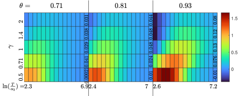
We fix and the priors . We vary , or equivalently taking the unit-free expression. We vary in a log-scaled range of .
5.2.1 Comparison with the bound
In [10], we showed the numerical inversions of LTs behave badly for large . Therefore, we sample the Monte-Carlo BB as follows. For each parameter grid, we simulate realizations of renewal processes with renewal process likelihood with IET density defined in (3.2). Let be the number of events for -th realization. We sum , only for realizations where all IETs or when . Then divide the summation by to get . Limit of space precludes derivation of the above sampling method.
We simulate the renewal processes conveniently by repeatedly generating IETs by inverse transform sampling until the next event time exceeds . In simulations, we observe that for the largest , the smallest , happening when , while the largest happening when .
We plot the sets of against and in the heat map in Fig. 1. We expect as . From Fig. 1, we have the following observations. (a) for large as expected. (b) The BB reaches its asymptotics faster for small and for away from , i.e. when class and are easier to distinguish. (c) We have to sample realizations to estimate reasonably well. However, the asymptotic expression is straightforward and much easier to interpret.
5.2.2 Comparison with the error probability
We have demonstrated our theorem by comparing with . However, one would also be interested in whether the error probability also has power decay like the bound. Hence, we simulate realizations of renewal processes for each class and carry out likelihood classification to sample the Monte-Carlo error probability .
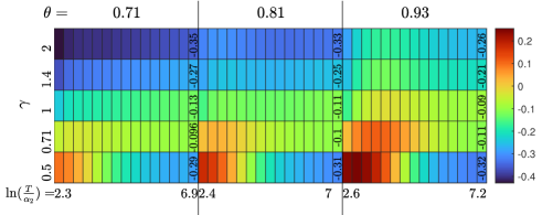
In simulations, for the largest , the smallest error probability happening when , while the largest error probability happening when .
We plot the heatmap of against and in Fig. 2. is an asymptotic relative discrepancy between the true error decay profile and the BB decay profile. If also has power decay, we expect constant as ; Fig. 2 confirms such property. We also have the following observations. (a) For small (or ), some because the asymptotic BB does not necessarily bound the error probability for small . However, the empirical BB does (see [10]). (b) For , has smaller absolute values for larger . This indicates that bounds the error decay profile better when and are closer. But for , the conclusion is the converse. (c) For fixed , bounds the error decay profile best for . (d) For , has not converged even with our largest observation time ; we need even longer observation time and thus also more realizations to sample the error probability decay profile. However, our asymptotic BB result is simple and takes almost no time to calculate.
6 Conclusions
In this paper, we developed, for the first time, the asymptotic approximation , of the Bhattacharyya bound (BB) for classifying renewal processes with heavy-tailed inter-event time distributions, based on Laplace transform analysis. We found that the BB has near power decay, indicating that the heavy-tailed renewal processes are harder to classify than the regular renewal processes whose BB decays exponentially. In the simulation studies, we compared with both the empirical BB and the empirical error probability .
In the future, we will consider more general classification settings, such as the ‘plugged-in’ likelihoods, subexponential distributions, and multiclass classification.
Appendix. Proof of the Main Theorem
Here, we prove Theorem 3. Under A1 and by Lemma 1, we have
| (A.1) |
We prove Theorem 3 in three steps, based on the value of .
Step 1: The asymptotic relation (4.1) is a direct application of the KT theorem.
Result 1: The relation (4.1) holds when .
Proof. For , the relation (A.1) and Theorem 2 give Then, note that . We have as . Now use Theorem 2 again to get (4.1).
Step 2: This case is not straightforward since (a) and (b) in Theorem 2 do not imply each other when . Thus, instead, we analyze the LT of . The LT exists on since is bounded by a polynomial with finite power. We need the following lemmas.
Lemma A: Let be slowly varying and locally bounded on and at . Then, at , where is slowly varying.
Proof. This is a generalization of [18, Proposition 1.5.9a]. The proof is simple and thus omitted.
Lemma B: , where is the density function whose survivor function is and is given in (3.2).
Proof. Use the hazard relations (2.1) to find .
Result 2: The relation (4.1) holds when .
Proof. Introduce . Then its LT . We have . So we examine and . First, is the LT of and , as , as . Now use Lemma A and Theorem 2 to get , as , as , where is slowly varying due to Lemma A and is the LT of . Then, due to Lemma B, we have for real , . This indicates that for ,
where is slowly varying and so we conclude by Lemma 1.
We thus find that dominates , so that , as , as , as , as needed.
Step 3: The KT theorem does not cover this case. We now need to analyze the LT of , where the integer satisfies
The LT also exists by the same arguments above. In this case, we need more results about the non-dominating LT terms. Let be the -th derivative of . The following lemmas hold.
Lemma C: For all integers , . (cf. [18, Proposition 1.5.10])
Lemma D: For all integers , .
Proof. It suffices to consider . The inequalities follow from Lemma B and Lemma C.
Result 3: The relation (4.1) holds when .
Proof. We need to discuss two cases.
First, for , let . Its LT has the term , and all other terms have finite limits as due to Lemma C and Lemma D. Then following the same as in the proof of Result 1 gives the quoted result.
Now consider and . We need to examine its LT terms with and , which are possibly infinite as . Following parallel steps from the proof of Result 2, using integral by parts to get, for , . We can also get that is slowly varying but . Then, we have that is slowly varying. However, the only term containing is , so it still dominates. The result then also follows easily.
Now Results 1-3 finally prove Theorem 3.
References
- [1] W. Bialek, R. R. Van Steveninck, F. Rieke, and D. Warland, Spikes: Exploring the Neural Code. MIT press, 1997.
- [2] P. Tankov and R. Cont, Financial Modelling with Jump Processes. Boca Raton: Chapman and Hall/CRC, 2004.
- [3] K. Zhou, H. Zha, and L. Song, “Learning social infectivity in sparse low-rank networks using multi-dimensional hawkes processes,” Journal of Machine Learning Research, vol. 31, pp. 641–649, 2013.
- [4] T. C. D. Shi, L. Shi, Event-Based State Estimation: A Stochastic Perspective,. New York: Springer, 2015.
- [5] M. Taniguchi, Asymptotic Theory of Statistical Inference for Time Series, ser. Springer series in statistics. New York: Springer-Verlag, 2000.
- [6] M. Lukasik, P. K. Srijith, D. Vu, K. Bontcheva, A. Zubiaga, and T. Cohn, “Hawkes processes for continuous time sequence classification: an application to rumour stance classification in Twitter,” in Proceedings of the 54th Annual Meeting of the Association for Computational Linguistics, Berlin, Germany, 2016, pp. 393–398.
- [7] J. Victor and K. Purpura, “Metric-space analysis of spike trains: Theory, algorithms and application,” Network: Computation in Neural Systems, vol. 8, no. 2, pp. 127–164, 1997.
- [8] A. Cholaquidis, L. Forzani, P. Llop, and L. Moreno, “On the classification problem for Poisson point processes,” Journal of Multivariate Analysis, vol. 153, 2015.
- [9] J. Mateu, F. Schoenberg, D. M. Diez, J. A. Gonzalez, and W. Lu, “On measures of dissimilarity between point patterns: Classification based on prototypes and multidimensional scaling,” Biometrical Journal, vol. 57, pp. 340–358, 2015.
- [10] X. Rong and V. Solo, “On the error rate for classifying point processes,” in 2021 60th IEEE Conference on Decision and Control (CDC), Austin, TX, USA, 2021, pp. 120–125.
- [11] M. Pawlak, M. Pabian, and D. Rzepka, “Asymptotically optimal nonparametric classification rules for spike train data,” in IEEE International Conference on Acoustics, Speech and Signal Processing, Rhodes Island, Greece, 2023, pp. 1–5.
- [12] ——, “Bayes risk consistency of nonparametric classification rules for spike trains data,” arXiv:2308.04796[cs.IT], 2023.
- [13] X. Rong and V. Solo, “Asymptotic error rates for point process classification,” arXiv:2403.12531[math.ST], 2024.
- [14] A. Clauset, C. R. Shalizi, and M. E. J. Newman, “Power-law distributions in empirical data,” SIAM Review, vol. 51, no. 4, pp. 661–703, 2009.
- [15] D. Daley and D. Vere-Jones, An Introduction to the Theory of Point Processes, 2nd ed. New York: Springer, 2003, vol. 1.
- [16] W. Feller, An Introduction to Probability Theory and its Applications. New York: J. Wiley, 1988, vol. 2.
- [17] S. Foss, D. Korshunov, and S. Zachary, An Introduction to Heavy-Tailed and Subexponential Distributions. Springer, 2011, vol. 6.
- [18] N. H. Bingham, C. M. Goldie, and J. L. Teugels, Regular Variation, ser. Encyclopedia of Mathematics and its Applications. Cambridge University Press, 1987.
- [19] J. Korevaar, Tauberian Theory: A Century of Developments. Berlin: Springer, 2004.