Clustering by Mining Density Distributions and Splitting Manifold Structure

Abstract

Spectral clustering requires the time-consuming decomposition of the Laplacian matrix of the similarity graph, thus limiting its applicability to large datasets. To improve the efficiency of spectral clustering, a top-down approach was recently proposed, which first divides the data into several micro-clusters (granular-balls), then splits these micro-clusters when they are not “compact”, and finally uses these micro-clusters as nodes to construct a similarity graph for more efficient spectral clustering. However, this top-down approach is challenging to adapt to unevenly distributed or structurally complex data. This is because constructing micro-clusters as a rough ball struggles to capture the shape and structure of data in a local range, and the simplistic splitting rule that solely targets “compactness” is susceptible to noise and variations in data density and leads to micro-clusters with varying shapes, making it challenging to accurately measure the similarity between them. To resolve these issues, this paper first proposes to start from local structures to obtain micro-clusters, such that the complex structural information inside local neighborhoods is well captured by them. Moreover, by noting that Euclidean distance is more suitable for convex sets, this paper further proposes a data splitting rule that couples local density and data manifold structures, so that the similarities of the obtained micro-clusters can be easily characterized. A novel similarity measure between micro-clusters is then proposed for the final spectral clustering. A series of experiments based on synthetic and real-world datasets demonstrate that the proposed method has better adaptability to structurally complex data than granular-ball based methods.

Introduction

Clustering is an unsupervised learning method aiming to reveal the intrinsic distribution characteristics of data by dividing the dataset into several non-overlapping clusters. It has wide applications in various fields such as computer vision (Tron et al. 2017), language processing (Zhang, Wang, and Shang 2023), and bioinformatics (Cheng and Ma 2022).

Spectral Clustering is a representative graph partition clustering algorithm, the core idea of which is to (approximately) minimize a cut loss of partitioning a similarity graph of data by removing some edges. It has attracted wide attention due to its exceptionally good performance in handling non-convex shaped clusters (von Luxburg 2007; Chen et al. 2011; He et al. 2019).

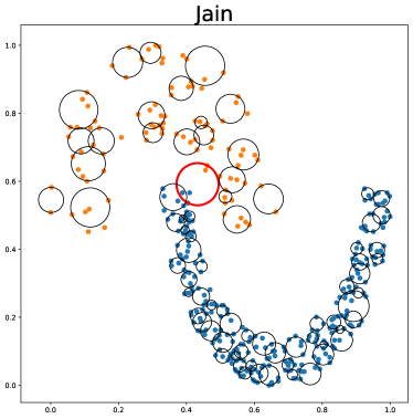
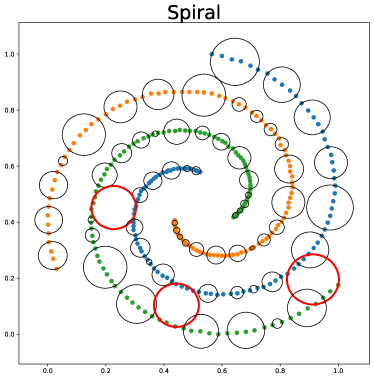
Figure 1: Illustration of errors (red circles) in granular-balls.

Spectral Clustering involves the spectral decomposition of the Laplacian matrix of a similarity graph, which has a prohibitively high complexity of $\mathcal{O}(n^{3})$ ($n$ represents the number of nodes in the graph) for large datasets. To improve the scalability, researchers have considered performing approximate spectral decomposition (Vladymyrov and Carreira-Perpiñán 2016), representing similarity between data approximately with anchors (Cai and Chen 2015; Huang et al. 2020), and constructing more sparse similarity graphs (Wu et al. 2018). These methods have different advantages and disadvantages, e.g., approximate decomposition needs to balance between efficiency and accuracy, and anchor-based ones are very sensitive to anchor numbers and positions. There is also research trying to fuse these directions (Yang et al. 2023).

Recently, Xie et al. (2023) proposed a new method called GBSC that progressively splits the data into micro-clusters (granular-balls) in a top-down manner, to obtain a coarse-grained representation of the original data, and then performs Spectral Clustering on balls representing several similar data points to reduce the size of the similarity graph. As each point is represented by a granular-ball, the overall structural information of data would be better captured than using the sampled anchors that is subject to missing the selection of some important anchors. This makes the granular-ball based approach very promising.

However, as it heavily relies on the quality of balls and the accuracy of the similarity measure between the balls, GBSC has two significant deficiencies for data of complex structures. Firstly, the splitting rule could produce low quality balls for complex data, because the rule only targets more “compact” balls and is based on a global view of data and a top-down manner. For example, in Fig. 1, when generating granular-balls from two clusters with significant density differences or manifold structure, some boundary points from different clusters are incorrectly grouped into the same granular-ball. Secondly, a granular-ball might contain data points distributed on a non-convex shape when the dataset is complex, and thus the Euclidean-based similarity between balls might no longer be appropriate.

To address these issues, this paper proposes another approach to represent data in a more coarse granularity. It first tries to capture more detailed local structural information of data by constructing micro-clusters from an estimation of data densities. Then it follows a more sophisticated splitting rule that also considers the convexity of data (called manifold curvature) to improve the quality of micro-clusters. The more convex distribution of data in micro-clusters also makes the design of similarity measure more straightforward and thus the final Spectral Clustering more effective.

The contributions of this paper are as follows:

• We propose a coarse-grained data representation scheme that combines local density estimation and convex splitting of local manifolds that is exploited to improve Spectral Clustering.

• Compared to granular-balls, the complex structures of data are better captured by extracting local density features to form a coarse-grained representation of data.

• Manifold curvature is introduced to split micro-clusters into more convex ones, which results in easier characterization of the intrinsic similarities between micro-clusters.

The rest of the paper is organized as follows. We first introduce the related work and review how granular-balls are generated, and then discuss the motivation and the framework of our algorithm, followed by experimental evaluations of the algorithm.

Related Work

The improvement and acceleration of Spectral Clustering has always been a focus in the field. Earlier, researchers explored numerical computation methods to accelerate spectral decomposition, e.g., the Nyström method (Fowlkes et al. 2004) efficiently approximates the spectral decomposition of a large Laplacian matrix by sampling data points. Later research (Vladymyrov and Carreira-Perpiñán 2016; Macgregor 2023) improved the sampling strategy and the representation ability to increase stability and reduce approximation error. However, these algorithms face the issue of balancing efficiency and approximation accuracy, and sampling-based schemes also have the problem of instability.

Another direction is to use anchors to characterize data, where the similarity between points are approximated using the similarity between point and anchors. Since the similarity graph between point and anchors is a bipartite graph, the spectral decomposition can be more efficient by working on a smaller matrix. For example, Cai and Chen (2015) performed K-means to obtain anchor points and constructed a sparsified bipartite graph between data points and these anchors by keeping only the connections of several nearest anchors for each point. Huang et al. (2020) further improved computational efficiency by first applying K-means on randomly sampled points to obtain anchors, then constructing a bipartite graph via fast approximate nearest neighbors, and finally performing transfer-cut on the bipartite graph for efficient spectral decomposition. There are also works (Gao et al. 2024; Nie et al. 2024) on combining anchors with the optimization process to increase efficiency.

Sparse similarity graphs can also be used to accelerate Spectral Clustering. For example, the SCRB method (Wu et al. 2018) used random binning features to generate inner products that approximate the similarity matrix of data, and employed singular value decomposition of large sparse matrices to improve the efficiency of spectral decomposition. The RESKM (Yang et al. 2023) framework tried to ensemble multiple strategies for more efficient Spectral Clustering.

Using micro-clusters to represent a group of data points was also a promising direction to reduce the size of data used for Spectral Clustering. The KASP method (Yan, Huang, and Jordan 2009) used K-means to group data points into micro-clusters and performed Spectral Clustering on the centers of these micro-clusters to reduce the size of similarity graph. The GBSC method (Xie et al. 2023) is a new and more sophisticated way to group data points into micro-clusters, by splitting the micro-clusters in a top-down manner to obtain a coarse-grained representation of the data, aiming for more compact micro-clusters. This method is combined with Spectral Clustering to achieve final clustering, while it can be combined with other clustering methods (Cheng et al. 2023) as well, demonstrating promising prospects. However, this top-down manner for a coarse-grained representation can result in micro-clusters of low quality which can distort the final clustering result. Therefore, this paper proposes a new micro-cluster construction strategy based on local structures, and also optimizes the splitting strategy to make the micro-clusters more convex and with high purity, to align with the needs of Spectral Clustering.

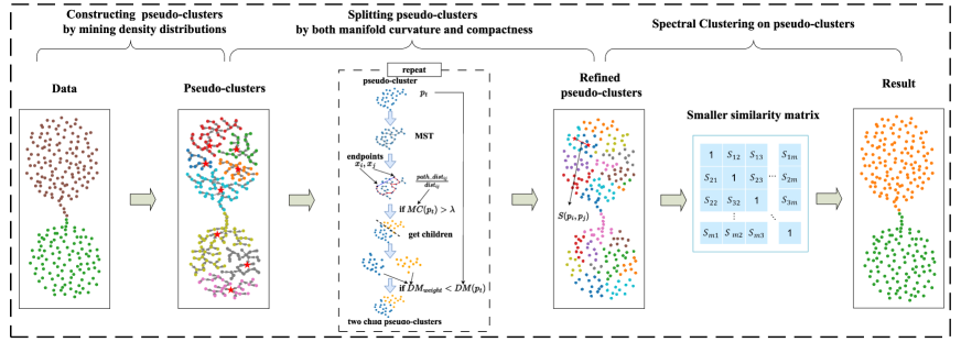
Figure 2: The framework of the proposed MDMSC algorithm.

Granular-Ball Generation

Given a dataset $X=\{x_{1},...,x_{n}\}$ $(x_{i}\in\mathbb{R}^{d})$, the target of GBSC (Xie et al. 2023) is to use a set of granular-balls as micro-clusters to cover the dataset, such that each data point belongs to a single granular-ball. A granular-ball is just an $d$ dimensional ball while the radius of the balls can vary from each other.

Specifically, suppose $GB_{j}$ is a granular-ball covering the $m$ data points $\{x_{i_{1}},\ldots,x_{i_{m}}\}\subseteq X$, then the center $c_{j}$ and the radius of $GB_{j}$ are determined as $c_{j}=\frac{1}{m}\sum_{s=1}^{m}x_{i_{s}}$ and $r_{j}=\max_{s}(\begin{Vmatrix}x_{i_{s}}-c_{j}\end{Vmatrix})$, where $||\cdot||$ denotes the $\ell_{2}$ norm. Note that if the radius of the granular-ball is large then the “granularity” is coarse and the clustering on the balls would be fast while much structural information would be lost; otherwise, the “granularity” is fine but clustering would be slow. Therefore, generating granular-balls needs to balance granularity and the quality of the balls.

In GBSC, the quality of a granular-ball $GB_{j}$ is defined as

$$DM_{j}=\frac{1}{m}\sum_{s=1}^{m}\|x_{i_{s}}-c_{j}\|.$$ (1)

$DM_{j}$ actually measures the “compactness” of the points within $GB_{j}$, where a smaller value of $DM_{j}$ means that the distance between the points is mostly small.

The generation of granular-balls in a top-down manner work as follows. First, a granular-ball $GB_{A}$ covering the entire dataset is generated. Then, two farthest points in $p_{1}$ and $p_{2}$ are selected, and the points in $GB_{A}$ are assigned to $p_{1}$ if they are closer to $p_{1}$ than to $p_{2}$. Two children balls $GB_{A_{1}}$ and $GB_{A_{2}}$ are then generated using the two subsets of points.

The core splitting strategy in GBSC is that if the weighted quality of the children balls is higher than that of the parent ball. Suppose $GB_{j_{1}}$ and $GB_{j_{2}}$ are the two children balls of $GB_{j}$, covering $m_{1}$ and $m_{2}$ points, respectively. Then the weighted quality of the children balls is

$$DM_{weight}=\frac{m_{1}}{m}DM_{j_{1}}+\frac{m_{2}}{m}DM_{j_{2}}.$$ (2)

For corner cases, GBSC also provides other splitting strategies including the restrictions on the number of points and the radius of a ball (see (Xie et al. 2023)). The above splitting process is repeated to generate final granular-balls until no more split can happen.

Algorithm

The splitting scheme of GBSC is performed in a top-down manner, and it does not consider local information, which can lead to incorrect splitting of local structures and thus affect the clustering performance.

To address these issues, we propose an improved algorithm MDMSC that initially partitions the dataset into multiple pseudo-clusters, instead of granular-balls, based on the density distribution of the data points, and then further split the pseudo-clusters based on structural characteristics. This approach aims to better capture the local features of the dataset and improve the clustering performance on complex datasets.

MDMSC consists of three stages: constructing pseudo-clusters as micro-clusters, splitting pseudo-clusters, and performing spectral clustering based on the similarity of the final pseudo-clusters. The algorithm framework is illustrated in Fig. 2.

Constructing Pseudo-Clusters

For each point $x_{i}$ in a dataset $X\in P^{n\times d}$, let $N_{k}(x_{i})$ be the set of the $k$ nearest neighbors of $x_{i}$ (excluding $x_{i}$ itself).

Before defining pseudo-clusters, we need to first define density and leader.

Definition 1.

The density $\rho(x_{i})$ of a point $x_{i}$, is defined as

$$\rho(x_{i})=\sum_{j=1}^{k}\exp(-dist_{ij}^{2}),$$ (3)

where $dist_{ij}$ refers to the Euclidean distance between point $x_{i}$ and its neighbor $x_{j}$.

The leader of each point $x_{i}$, denoted as $\mathsf{leader}(x_{i})$, is defined as the nearest higher-density point of $x_{i}$.

Definition 2.

The leader of a point $x_{i}$ is

$$\mathsf{leader}(x_{i})=\left\{\begin{array}[]{ll}\mathop{\text{argmin}}\limits_{x_{j}\in\mathcal{H}(x_{i})}{dist_{ij}}&\text{if $\mathcal{H}(x_{i})\neq\emptyset$}\\ \text{None}&\text{otherwise}\end{array}\right.$$ (4)

where the set $\mathcal{H}(x_{i})=\{x_{j}\mid x_{j}\in N_{k}(x_{i}),\rho(x_{j})>\rho(x_{i})\}$. Points without a leader are called core points, and the set of core points is denoted as $\mathsf{core}=\{x_{i}\mid\mathsf{leader}(x_{i})=\text{None}\}$.

Definition 3 (Pseudo-cluster).

Let $G=(X,E)$ be a directed graph, where $(x_{i},x_{j})\in E$ if $x_{j}$ is the leader of $x_{i}$. A pseudo-cluster is a connected component of $G$.

Pseudo-clusters are actually a local tree structure, where its root is a core point. By considering density distributions, a local tree structure has high purity and can thus better reflect local structures of data than granular-balls.

Intuitively, by connecting each point $x_{i}$ to its leader $\mathsf{leader}(x_{i})$, multiple disjoint pseudo-clusters are formed, with each pseudo-cluster being defined by the unique core point within the pseudo-cluster. Algorithm 1 shows the steps of constructing pseudo-clusters.

Fig. 3 illustrates the pseudo-clusters of Jain with $k=10$ and Spiral with $k=4$. It can be seen that pseudo-clusters better reflects the local characteristics of the dataset, and the problem of a granular-ball in Fig. 1 containing points from different clusters has been rectified.

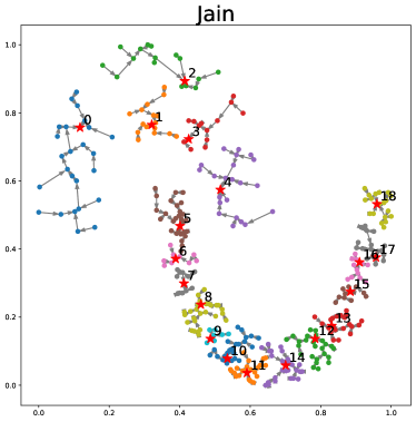
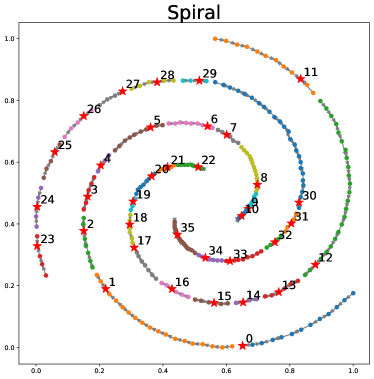
Figure 3: Illustration of pseudo-clusters and their complex structures.

Algorithm 1 Constructing pseudo-clusters

0:  Dataset X, and the number of nearest neighbors $k$.

0:  Pseudo-clusters $\mathsf{pseudo}\_\mathsf{clusters}$.

1:  for each $x_{i}\in X$ do

2:     Calculate $N_{k}(x_{i})$;

3:     Calculate $\rho(x_{i})$;

4:  end for

5:  $\mathsf{core}\leftarrow\emptyset$;

6:  for each $x_{i}\in X$ do

7:     Calculate $\mathsf{leader}(x_{i})$;

8:     if $\mathsf{leader}(x_{i})$ = None then

9:         $\mathsf{core}\leftarrow\mathsf{core}\cup\{x_{i}\}$;

10:     end if

11:     Connect $x_{i}$ and $\mathsf{leader}(x_{i})$;

12:  end for

13:  Identify $\mathsf{pseudo}\_\mathsf{clusters}$ as connected components;

14:  return $\mathsf{pseudo}\_\mathsf{clusters}$

Splitting Pseudo-Clusters

Although the pseudo-clusters reflect the basic distribution of the data, these pseudo-clusters may be too coarse for the entire dataset. Additionally, pseudo-clusters have various shapes and structures, many of which are non-convex, which makes measuring the similarity between pseudo-clusters difficult.

On the left side of Fig. 3, the pseudo-clusters of numbers 0, 1, 2, 3, and 8 exhibit non-convex structures and complex shapes, and the distance between these pseudo-clusters and others can not be easily measured with Euclidean based distances. For example, for pseudo-cluster 2, although its core point is close to pseudo-cluster 1, the points in the left part of it is far away. The situation is similar on the other side.

To address this issue, we need to split the pseudo-clusters into simpler convex structures. We introduce the measurement of manifold curvature to better determine if a pseudo-cluster is too “curved”.

Definition 4 (Manifold curvature).

Suppose $p_{t}$ is a pseudo-cluster, and $T(p_{t})$ is a minimum spanning tree (MST) of the complete weighted graph for the points in $p_{t}$, where the weights of the edges are the Euclidean distances between the points. The manifold curvature of a pseudo-cluster $p_{t}$ is

$$MC(p_{t})=\frac{path\_dist_{ij}}{dist_{ij}}\ (x_{i},x_{j}=\mathsf{endpoints}(p_{t})),$$ (5)

where $path\_dist$ is the shortest path distance between points on $T(p_{t})$, and $\mathsf{endpoints}(p_{t})=\operatorname{argmax}_{x_{i},x_{j}\in p_{t}}path\_dist_{ij}$.

Intuitively, in a pseudo-cluster, the shortest path distance reflects the geodesic distance between points, while the Euclidean distance represents the “direct” distance between them. Thus, we define the manifold curvature as the ratio of the shortest path distance to the Euclidean distance between the endpoints. The larger the ratio is, the more “curved” the pseudo-cluster will be. When the ratio approaches 1, the data will be nearly convex.

By splitting pseudo-clusters under the measurement of manifold curvature, we can ensure that the pseudo-clusters have stronger convexity, making the consideration of pseudo-cluster compactness more reasonable and also beneficial for capturing the intrinsic similarities.

To determine whether a pseudo-cluster $p_{t}$ should be split, we consider both the manifold curvature and the compactness of the original pseudo-cluster and its child pseudo-clusters according to Eq. 1 and Eq. 2. In particular, if $MC(p_{t})\geq\lambda$ and $DM_{weight}<DM(p_{t})$, then $p_{t}$ will be split. In order to avoid too small pseudo-clusters, we also require $p_{t}$ should contain a minimum number $\beta$ of points, as in (Xie et al. 2023).

When a pseudo-cluster needs to be split, its two endpoints $\mathsf{endpoints}(p_{t})$ will be used to construct the new child pseudo-clusters, where the other points in $p_{t}$ are assigned to the new pseudo-clusters based on proximity to the endpoints. The process will be repeated until none of the pseudo-clusters can be split.

Algorithm 2 MDMSC

0:  Dataset $X$, the number of nearest neighbors $k$, the manifold curvature threshold $\lambda$, and the mimum size of pseudo-cluster $\beta$.

0:  Final clustering labels.

1:  Get $\mathsf{pseudo}\_\mathsf{clusters}$ by Algorithm 1;

2:  for each $p_{t}\in\mathsf{pseudo}\_\mathsf{clusters}$ do

3:     Generate a complete undirected graph $G(p_{t})$;

4:     Generate an MST $T(p_{t})$ from $G(p_{t})$;

5:     for $x_{i},x_{j}\in p_{t}$ do

6:        Calculate $path\_dist_{ij}$ on $T(p_{t})$;

7:     end for

8:  end for

9:  while $\exists p_{t}$ s.t. $MC(p_{t})>\lambda$ and $DM_{weight}<DM(p_{t})$ and $|p_{t}|>\beta$ do

10:     Split $p_{t}$ into $p_{t_{1}}$ and $p_{t_{2}}$ and add them to $\mathsf{pseudo}\_\mathsf{clusters}$;

11:  end while

12:  Calculate similarity matrix $S$;

13:  Perform Spectral Clustering on the $S$ to obtain final clustering results.

Clustering Pseudo-Clusters

After obtaining the final pseudo-clusters, the next step is to establish similarity between pseudo-clusters and ultimately perform clustering through graph partitioning Here, we employ spectral clustering on pseudo-clusters.

Since the pseudo-clusters are approximately convex now, it is straightforward to use Euclidean distance to evaluate their similarity, as follows.

Definition 5 (Similarity).

The similarity of two pseudo-clusters $p_{i}$ and $p_{j}$ is

$$S(p_{i},p_{j})=\frac{|\mathsf{SNN}(p_{i},p_{j})|}{1+c\_dist(p_{i},p_{j})},$$ (6)

where $\mathsf{SNN}(p_{i},p_{j})=\cup_{x\in p_{i}}N_{k}(x)\cap\cup_{x\in p_{j}}N_{k}(x)$ is the shared nearest neighbors of $p_{i}$ and $p_{j}$, and $c\_dist(p_{i},p_{j})$ is the Euclidean distance between the centroids of $p_{i}$ and $p_{j}$. A centroid of $p_{i}$ is $\frac{1}{m_{i}}\sum_{x\in p_{i}}x$, which is not necessarily a core point.

Subsequently, we perform Spectral Clustering on the similarity matrix of the pseudo-clusters. Points within the same pseudo-cluster will be assigned the same cluster label. The full steps of the proposed algorithm MDMSC is given in Algorithm 2.

Time Complexity

Suppose the dataset $X$ has $n$ samples with the dimensionality of $d$, the final number of pseudo-clusters is $m$, and the number of nearest neighbors is $k$. In Algorithm 1, the time complexity for finding k-nearest neighbors using the KD-tree method is $\mathcal{O}((k+n)\log n)$, the time complexity for calculating density is $\mathcal{O}(kn)$, and the time complexity for finding the leader point of a data point is $\mathcal{O}(kn)$.

In Algorithm 2, suppose the number of samples in each pseudo-cluster is $n_{i}$, for each pseudo-cluster, the time complexity for creating a complete graph is $\mathcal{O}(n_{i}^{2})$, for obtaining the minimum spanning tree from the complete graph using Kruskal’s algorithm is $\mathcal{O}(n_{i}^{2}\log n_{i})$, and for calculating the shortest path distances between any two points in the pseudo-cluster using Dijkstra’s algorithm is $\mathcal{O}(n_{i}^{2}\log n_{i})$. The total time complexity for splitting all existing pseudo-clusters once is $\sum_{i}\mathcal{O}(n_{i}^{2}\log n_{i})$, where $\sum_{i}n_{i}=n$. The time complexity for spectral clustering is $\mathcal{O}(m^{3})$.

Actually, $\sum_{i}\mathcal{O}(n_{i}^{2}\log n_{i})$ is bounded by $\mathcal{O}(nn_{*}\log n_{*})$, where $n_{*}$ is the maximum of $n_{i}$, as shown in the following theorem (see supplementary material for proof). Therefore, the overall time complexity of the algorithm is thus $\mathcal{O}(nn_{*}(\log n_{*})^{2}+m^{3})$.

Theorem 1.

Suppose there are $l$ pseudo-clusters. Let $n=\sum_{i=1}^{l}n_{i}$, where $n_{i}\geq 1$ is the number of points in a pseudo-cluster $p_{i}$. Then $\sum_{i}n_{i}^{2}\log n_{i}=\mathcal{O}(nn_{*}\log{n_{*}})$, where $n_{*}$ is the maximum of $n_{i}$.

Experiments

Experimental Setup

We used three evaluation metrics: ARI (Steinley 2004), NMI (Xu, Liu, and Gong 2003), and ACC (Yang et al. 2010) for clustering analysis. Since the proposed algorithm is based on local density peaks and pseudo-cluster splitting followed by spectral clustering, we selected the following eight comparison algorithms: GBSC (Xie et al. 2023), GB-DP (Cheng et al. 2023), LDP-MST (Cheng et al. 2021), USPEC (Huang et al. 2020), SC (Shi and Malik 2000), DPC (Rodriguez and Laio 2014), DEMOS (Guan et al. 2023), and DPC-DBFN (Lotfi, Moradi, and Beigy 2020).

For MDMSC, we searched for $k$ in the range of 2 to 50 and for $\beta$ in $\{8,16\}$, and the threshold $\lambda$ was set to $1.5$. The implementation details of other algorithms are provided in the supplementary material.

Dataset	#Instance	#Attributes	#Clusters
border	840	892	3
mfea-fac	2000	216	10
Kdd9	1280	41	3
landsatEW	6435	36	6
balance-scale	625	4	3
pengleukEW	72	7070	2
Pendigits	10992	16	10
energy-y2	766	8	3
optical_test	1797	62	10
soybean_test	376	35	18
car	1728	6	4
semeionEW	1593	256	10
vote	435	16	2

Table 1: Real-world datasets.

In terms of datasets, we used 4 synthetic datasets and 13 real-world datasets (Table 1). All datasets were normalized, and the results were averaged over 10 runs.

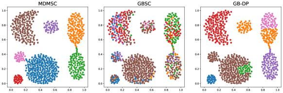
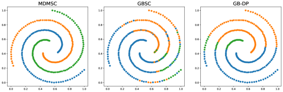
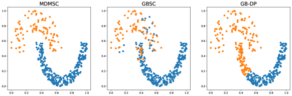
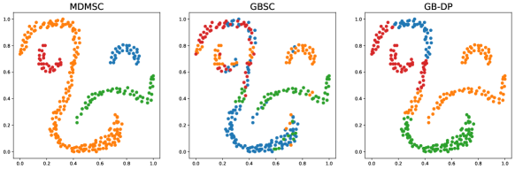
Figure 4: Visualizations on synthetic datasets.

Visualizations on Synthetic Datasets

We present visualizations of several datasets with obvious manifold structures in Fig. 4, where MDMSC performs well, while GBSC and GB-DP misclassify points within the same cluster. For example, GBSC misclassifies many isolated points into incorrect clusters due to the granular-ball splitting process and its simplistic similarity measure. On the other hand, MDMSC, by leveraging local density features and considering manifold curvature, effectively captures complex shapes and manifold structures.

Dataset		MDMSC	GBSC	GB-DP	LDP-MST	USPEC	SC	DPC	DEMOS	DPC-DBFN
border	ARI	19.54	0.01	16.70	1.18	17.35	17.48	8.73	14.20	2.83
	NMI	18.59	0.34	15.17	1.89	16.15	15.58	10.92	14.66	6.10
	ACC	56.67	44.39	49.76	45.00	53.46	51.90	49.52	52.50	45.59
mfea-fac	ARI	86.28	24.92	39.78	61.50	84.57	85.57	59.85	75.58	48.80
	NMI	87.54	42.58	58.79	72.41	86.39	87.31	74.43	82.57	69.11
	ACC	93.45	41.30	61.90	72.15	92.56	93.00	65.85	87.30	59.10
Kdd9	ARI	96.53	5.67	84.93	86.08	70.71	52.16	0.05	NA	3.02
	NMI	96.09	7.96	85.98	85.79	73.08	62.55	0.36	NA	13.75
	ACC	97.97	41.67	94.53	95.00	86.55	73.85	38.83	NA	46.56
landsatEW	ARI	56.45	49.17	34.48	50.01	58.36	47.23	46.18	NA	4.68
	NMI	63.50	56.53	47.45	59.83	65.16	60.42	56.06	NA	10.40
	ACC	70.16	67.61	55.63	64.21	70.50	63.66	71.75	NA	30.58
balance-scale	ARI	24.60	5.25	10.31	0.91	11.10	13.57	15.07	NA	11.14
	NMI	22.66	5.44	8.91	6.63	9.33	12.15	11.73	NA	10.42
	ACC	60.16	51.70	52.48	49.92	51.94	54.24	54.40	NA	54.40
pengleukEW	ARI	35.85	2.96	23.79	32.90	29.75	26.63	10.52	26.00	15.95
	NMI	25.07	5.95	17.13	24.06	21.96	18.95	14.39	16.98	10.73
	ACC	80.56	58.61	75.00	79.16	77.78	76.39	70.83	76.38	70.83
Pendigits	ARI	77.81	42.62	51.91	70.11	71.05	76.24	63.50	70.53	49.91
	NMI	84.85	59.72	67.51	81.66	81.52	83.73	75.41	80.75	67.67
	ACC	88.08	57.17	63.05	78.02	82.98	87.17	75.63	84.18	64.55
energy-y2	ARI	70.65	4.57	69.17	70.58	35.24	70.58	55.17	45.58	65.29
	NMI	66.44	5.55	68.97	66.40	47.02	66.40	62.13	58.11	66.67
	ACC	80.86	51.07	74.09	80.73	55.95	80.73	65.76	49.86	71.61
optical_test	ARI	84.08	28.70	32.52	56.37	80.84	81.47	72.25	82.27	-0.06
	NMI	90.13	51.58	59.44	75.04	88.06	89.91	83.41	87.90	0.83
	ACC	89.43	52.08	55.15	65.77	86.69	87.82	78.69	89.14	10.51
soybean_test	ARI	43.04	29.26	31.26	39.89	39.11	46.22	32.72	31.30	35.13
	NMI	75.08	59.03	65.55	67.21	74.81	69.46	64.65	59.82	58.29
	ACC	64.10	44.55	42.82	53.98	60.61	56.41	46.01	44.95	50.80
car	ARI	40.44	-3.08	4.90	11.40	17.19	17.79	15.90	9.16	14.46
	NMI	28.51	5.28	11.13	32.40	24.57	25.04	30.47	15.73	10.36
	ACC	69.44	57.25	35.94	55.55	47.39	47.96	51.56	46.81	61.57
semeionEW	ARI	52.62	0.53	23.28	26.79	48.34	44.81	19.63	33.19	26.03
	NMI	67.45	5.85	42.15	52.15	64.66	64.29	35.20	55.53	42.59
	ACC	68.30	13.21	41.68	47.70	62.82	58.59	36.97	45.26	39.30
vote	ARI	57.10	-0.83	53.67	20.57	0.37	55.72	53.00	NA	45.07
	NMI	49.93	8.32	45.98	24.44	0.31	48.40	45.95	NA	33.92
	ACC	87.82	55.08	86.67	72.87	61.61	87.36	86.44	NA	83.67

Table 2: Results on real-world datasets (%).

Results on Real-World Datasets

Table 2 shows the results (bold means best) of our algorithm and the other eight comparison algorithms on real-world datasets. MDMSC achieves the best performance on most datasets. For example, on the high-dimensional dataset pengleukEW, MDMSC significantly outperforms most comparison algorithms. We attribute this to the consideration of manifold curvature, allowing it to effectively handle complex high-dimensional datasets. Additionally, on the large-scale dataset Pendigits, our algorithm also shows superior performance, demonstrating its capability to effectively handle large-scale datasets by partitioning pseudo-clusters. Although our algorithm does not always achieve the best results on a few datasets like landsatEW and soybean_test, its performance is very close to the optimal ones. This indicates that our algorithm possesses strong adaptability and effectiveness across a wide range of application scenarios.

We also performed Friedman test and subsequent Nemenyi test on the ACC results. Friedman test showed that there exists significant differences ($p<0.05$) between the results and Nemenyi test confirmed that our algorithm significantly outperforms all of the other algorithms: $CD=2.10$ and the rank differences of MDMSC with other algorithms are all larger than $2.10$.

Ablation Study

To demonstrate the effectiveness of each component of our algorithm, we conducted ablation studies on 7 real-world datasets. The best results are presented in Table 3 by tuning hyperparameters. The columns $a$, $b$, and $c$ represent the following different settings, respectively:

1. Directly uses the whole dataset as the initial pseudo-cluster, without using Algorithm 1.

2. Does not further split the pseudo-clusters.

3. Only uses compactness to split the pseudo-clusters.

The results indicate that the performance of the algorithm decreases when a specific component is removed. Setting $a$ demonstrates that extracting local density features helps characterize the data distribution. Settings $b$ and $c$ show that considering manifold curvature is beneficial for the quality of pseudo-clusters.

Dataset	MDMSC	$a$	$b$	$c$
mfea-fac	86.28	71.28	71.72	84.40
Kdd9	96.53	84.93	84.93	96.53
balance-scale	24.60	14.40	19.61	22.46
pengleukEW	35.85	29.61	-5.84	23.79
optical_test	84.08	63.56	78.11	81.53
semeionEW	52.62	34.90	46.57	48.12
vote	57.10	54.34	53.00	53.00

Table 3: Ablation study results (%).

Robustness Analysis

Fig. 5 evaluates the performance variation of the algorithm under different hyperparameter settings, we tested it on multiple datasets. shows the ARI variations of our algorithm, SC, and DPC-DBFN algorithms on datasets optical_test, Pendigits, Kdd9, and mfea-fac. The results indicate that our algorithm experiences larger fluctuations with smaller $k$ values on the Pendigits and Kdd9 datasets, but the ARI values stabilize as $k$ increases. Furthermore, our algorithm is relatively stable on the optical_test and mfeafac datasets. This suggests that our algorithm exhibits a certain degree of robustness to changes in $k$ values and maintains high performance across most datasets.

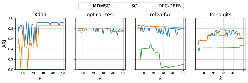
Figure 5: Impacts of $k$ on clustering performance.

Running Time

Fig. 6 compares the running time and ACC of our algorithm with GBSC. The proposed MDMSC has shorter run time than GBSC on 7 out of 13 datasets and similar run time on most of the other datasets, and on all of these datasets, MDMSC has higher ACC than GBSC. The reason for the slower cases is that we make use of more complex micro-clusters to represent data and the splitting rule is also more sophisticated, and it is actually worthy in most of the cases.

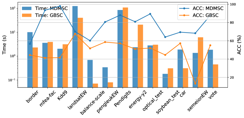
Figure 6: Time and ACC comparison.

Conclusion

The paper proposes a new approach to represent data in a coarse granularity that can accelerate and improve the performance of Spectral Clustering. Specifically, the approach can discover micro-clusters based on local density distributions of data, and introduces the concept of manifold curvature of micro-clusters to help split them into more convex ones. In this way, the approach provides better representation of data and simplifies the characterization of the similarities, resulting in better performance in subsequent Spectral Clustering. Evaluations on 4 synthetic datasets and 13 real-world datasets, against relevant state-of-the-art algorithms, show that the proposed algorithm performs best on most datasets. The ablation experiments also demonstrated the effectiveness of the proposed components.

Despite the impressive performance of the proposed algorithm in the experiments, there is still room for improvement and optimization. Future work will attempt to introduce more efficient computational techniques, such as parallel and distributed computing, to further enhance the computational speed of the algorithm, especially when handling ultra-large-scale datasets. Additionally, one can consider developing adaptive hyperparameter optimization methods for this approach, and can also consider to combine it with other clustering methods.

References

- Cai and Chen (2015) Cai, D.; and Chen, X. 2015. Large Scale Spectral Clustering Via Landmark-Based Sparse Representation. IEEE Trans. Cybern., 45(8): 1669–1680.
- Chen et al. (2011) Chen, W.; Song, Y.; Bai, H.; Lin, C.; and Chang, E. Y. 2011. Parallel Spectral Clustering in Distributed Systems. IEEE Trans. Pattern Anal. Mach. Intell., 33(3): 568–586.
- Cheng et al. (2023) Cheng, D.; Li, Y.; Xia, S.; Wang, G.; Huang, J.; and Zhang, S. 2023. A fast granular-ball-based density peaks clustering algorithm for large-scale data. IEEE Trans. Neural Networks Learn. Syst, 1–14.
- Cheng et al. (2021) Cheng, D.; Zhu, Q.; Huang, J.; Wu, Q.; and Yang, L. 2021. Clustering with Local Density Peaks-Based Minimum Spanning Tree. IEEE Trans. Knowl. Data Eng., 33(2): 374–387.
- Cheng and Ma (2022) Cheng, Y.; and Ma, X. 2022. scGAC: a graph attentional architecture for clustering single-cell RNA-seq data. Bioinform., 38(8): 2187–2193.
- Fowlkes et al. (2004) Fowlkes, C. C.; Belongie, S. J.; Chung, F. R. K.; and Malik, J. 2004. Spectral Grouping Using the Nyström Method. IEEE Trans. Pattern Anal. Mach. Intell., 26(2): 214–225.
- Gao et al. (2024) Gao, C.; Chen, W.; Nie, F.; Yu, W.; and Wang, Z. 2024. Spectral clustering with linear embedding: A discrete clustering method for large-scale data. Pattern Recognit., 151: 110396.
- Guan et al. (2023) Guan, J.; Li, S.; Chen, X.; He, X.; and Chen, J. 2023. DEMOS: Clustering by Pruning a Density-Boosting Cluster Tree of Density Mounts. IEEE Trans. Knowl. Data Eng., 35(10): 10814–10830.
- He et al. (2019) He, L.; Ray, N.; Guan, Y.; and Zhang, H. 2019. Fast Large-Scale Spectral Clustering via Explicit Feature Mapping. IEEE Trans. Cybern., 49(3): 1058–1071.
- Huang et al. (2020) Huang, D.; Wang, C.; Wu, J.; Lai, J.; and Kwoh, C. 2020. Ultra-Scalable Spectral Clustering and Ensemble Clustering. IEEE Trans. Knowl. Data Eng., 32(6): 1212–1226.
- Lotfi, Moradi, and Beigy (2020) Lotfi, A.; Moradi, P.; and Beigy, H. 2020. Density peaks clustering based on density backbone and fuzzy neighborhood. Pattern Recognit., 107: 107449.
- Macgregor (2023) Macgregor, P. 2023. Fast and Simple Spectral Clustering in Theory and Practice. In NeurIPS, 34410–34425.
- Nie et al. (2024) Nie, F.; Xue, J.; Yu, W.; and Li, X. 2024. Fast Clustering With Anchor Guidance. IEEE Trans. Pattern Anal. Mach. Intell., 46(4): 1898–1912.
- Rodriguez and Laio (2014) Rodriguez, A.; and Laio, A. 2014. Clustering by fast search and find of density peaks. Science, 344(6191): 1492–1496.
- Shi and Malik (2000) Shi, J.; and Malik, J. 2000. Normalized Cuts and Image Segmentation. IEEE Trans. Pattern Anal. Mach. Intell., 22(8): 888–905.
- Steinley (2004) Steinley, D. 2004. Properties of the hubert-arable adjusted rand index. Psychological Methods, 9(3): 386.
- Tron et al. (2017) Tron, R.; Zhou, X.; Esteves, C.; and Daniilidis, K. 2017. Fast Multi-image Matching via Density-Based Clustering. In ICCV, 4077–4086.
- Vladymyrov and Carreira-Perpiñán (2016) Vladymyrov, M.; and Carreira-Perpiñán, M. Á. 2016. The Variational Nystrom method for large-scale spectral problems. In ICML, volume 48, 211–220.
- von Luxburg (2007) von Luxburg, U. 2007. A tutorial on spectral clustering. Stat. Comput., 17(4): 395–416.
- Wu et al. (2018) Wu, L.; Chen, P.; Yen, I. E.; Xu, F.; Xia, Y.; and Aggarwal, C. C. 2018. Scalable Spectral Clustering Using Random Binning Features. In SIGKDD, 2506–2515.
- Xie et al. (2023) Xie, J.; Kong, W.; Xia, S.; Wang, G.; and Gao, X. 2023. An Efficient Spectral Clustering Algorithm Based on Granular-Ball. IEEE Trans. Knowl. Data Eng., 35(9): 9743–9753.
- Xu, Liu, and Gong (2003) Xu, W.; Liu, X.; and Gong, Y. 2003. Document clustering based on non-negative matrix factorization. In SIGIR, 267–273.
- Yan, Huang, and Jordan (2009) Yan, D.; Huang, L.; and Jordan, M. I. 2009. Fast approximate spectral clustering. In SIGKDD, 907–916.
- Yang et al. (2023) Yang, G.; Deng, S.; Chen, X.; Chen, C.; Yang, Y.; Gong, Z.; and Hao, Z. 2023. RESKM: A General Framework to Accelerate Large-Scale Spectral Clustering. Pattern Recognit., 137: 109275.
- Yang et al. (2010) Yang, Y.; Xu, D.; Nie, F.; Yan, S.; and Zhuang, Y. 2010. Image Clustering Using Local Discriminant Models and Global Integration. IEEE Trans. Image Process., 19(10): 2761–2773.
- Zhang, Wang, and Shang (2023) Zhang, Y.; Wang, Z.; and Shang, J. 2023. ClusterLLM: Large Language Models as a Guide for Text Clustering. In EMNLP, 13903–13920.