Achieving the Tightest Relaxation of Sigmoids for Formal Verification
Abstract
In the field of formal verification, Neural Networks (NNs) are typically reformulated into equivalent mathematical programs which are optimized over. To overcome the inherent non-convexity of these reformulations, convex relaxations of nonlinear activation functions are typically utilized. Common relaxations (i.e., static linear cuts) of “S-shaped” activation functions, however, can be overly loose, slowing down the overall verification process. In this paper, we derive tuneable hyperplanes which upper and lower bound the sigmoid activation function. When tuned in the dual space, these affine bounds smoothly rotate around the nonlinear manifold of the sigmoid activation function. This approach, termed -sig, allows us to tractably incorporate the tightest possible, element-wise convex relaxation of the sigmoid activation function into a formal verification framework. We embed these relaxations inside of large verification tasks and compare their performance to LiRPA and -CROWN, a state-of-the-art verification duo.
Introduction
Formal verification has an ever-widening spectrum of important uses, including mathematical proof validation (Trinh et al. 2024), adversarially robust classification (Zhang et al. 2022a), data-driven controller reachability analysis (Everett 2021), performance guarantees for surrogate models of the electric power grid (Chevalier and Chatzivasileiadis 2024), and more (Urban and Miné 2021). The formal verification of Neural Networks (NNs), in particular, has seen a flurry of recent research activity. Pushed by the international Verification of Neural Networks Competition (VNN-Comp), NN verification technologies have scaled rapidly in recent years (Brix et al. 2023b, a). Competitors have exploited, and synergistically spurred, the development of highly successful verification algorithms, e.g., -CROWN (Wang et al. 2021; Lyu et al. 2019), Multi-Neuron Guided Branch-and-Bound (Ferrari et al. 2022), DeepPoly (Singh et al. 2019), etc. The winningest methods emerging from VNN-Comp serve as the leading bellwethers for state-of-the-art within the NN verification community.
Despite these advances, verification technologies cannot yet scale to Large Language Model (LLM) sized systems (Sun et al. 2024). Nonlinear, non-ReLU activation functions present one of the key computational obstacles which prevents scaling. While these activation functions can be attacked with spatial Branch-&-Bound (B&B) approaches (Shi et al. 2024), authors in (Wu et al. 2023) note that “existing verifiers cannot tightly approximate S-shaped activations.” The sigmoid activation is one such S-shaped activation function which is challenging to deal with. Given its close relationship to the ubiquitous softmax function (Wei et al. 2023), which is embedded in modern transformer layers (Ildiz et al. 2024), efficient verification over the sigmoid activation function would help boost verification speeds and generally help extend verification technology applicability.
Our contributions. Given the ongoing computational challenge of verifying over NNs containing sigmoid activation fucntions, our contributions follow:
-
1.
We derive an explicit mapping between the linear slope and y-intercept point of a tangent line which tightly bounds a sigmoid. This differentiable, tunable mapping is embedded into a verification framework to yield the tightest possible element-wise relaxation of the sigmoid.
-
2.
We propose a “backward” NN evaluation routine which dynamically detects if a sigmoid should be upper or lower bounded at each step of a gradient-based solve.
-
3.
To ensure feasible projection in the dual space, we design a sequential quadratic program which efficiently pre-computes maximum slope bounds of all tunable slopes.
Many verification algorithms exploit element-wise convex relaxation of nonlinear activation functions, resulting in convex solution spaces (Salman et al. 2020). The stacking up of tightening dual variables within a dualized problem reformulation, as in -CROWN, can lead to a formally nonconvex mathematical program. Similarly, the verification formulation which we present in this paper is nonconvex, but it globally lower bounds the true verification solution. Authors in (Bunel et al. 2020) have shown that spurious local minima in nonconvex problems containing “staged convexity” are very rare, and they even design perturbation-based approaches to avoid them. In this paper, we use a gradient-based approach to solve a formally nonconvex problem, but solutions smoothly converge to what appears to be a global maximum.
Related Works
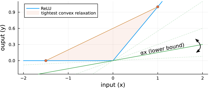
To iteratively tighten relaxed ReLU-based NNs, the architects of -CROWN (Xu et al. 2021) use the “optimizable” linear relaxation demonstrated in Fig. 1. In this approach, the parameter is tuned to achieve a maximally tight lower bound on the verification problem. Authors in (Salman et al. 2020) showed variables to be equivalent to the dual variables of an associated linear program (LP)-relaxed verification problem. (Wang et al. 2021) applied the -CROWN approach within a B&B context, introducing new split-constraint dual variables to be optimized over in the dual space. More recently, (Shi et al. 2024) developed a general framework (GenBaB) to perform B&B over a wide class of nonlinear activations, including sigmoid, tanh, sine, GeLU, and bilinear functions. The authors utilize pre-optimized branching points in order to choose linear cuts which statically bound portions of the activation functions. Critically, they also incorporate optimizable linear relaxations of the bilinear, sine, and GeLU activation functions using -like tunable parameters.
Verification over “S-shaped” activation functions is considered in (Wu et al. 2023), where the authors use sequential identification of counterexamples in the relaxed search space to iteratively tighten the activation relaxations. Authors in (Zhang et al. 2022b) propose a verification routine which incorporates the provably tightest linear approximation of sigmoid-based NNs. Notably, the approach uses static (i.e., non-tunable) linear approximations, improving upon other works whose sigmoid relaxations minimize relaxation areas (Henriksen and Lomuscio 2020) or use parallel upper and lower bounding lines (Wu and Zhang 2021). While existing approaches have designed advanced cut selection procedures for sigmoid activation functions, and even embedded these procedures within B&B, there exists no explicitly optimizable, maximally tight linear relaxation strategy for sigmoid activation functions.
Formal Verification Framework
Let be the input to an -layer NN mapping . A scalar verification metric function, , wraps around the NN to generate the verification function . This metric is defined such that the NN’s performance is verified if , , can be proved:
| (1) |
In this NN, is the layer linear transformation, with as the input, and is the associated nonlinear activation. In this paper, exclusively represents the sigmoid activation function:
| (2) |
where the gradient of the sigmoid is . As in (Wang et al. 2021), the region can be described as an norm ball constraint on the input via . To solve (1) to global optimality (or, at least, to prove ), many recent approaches have utilized () convex relaxation of activation functions coupled with () spatial (Shi et al. 2024) and discrete (Wang et al. 2021) Branch-and-Bound (B&B) strategies. B&B iteratively toggles activation function statuses, yielding tighter and tighter solutions, in pursuit of the problem’s true lower bound. In this paper, we exclusively consider the so-called root node relaxation of (1), i.e., the first, and generally loosest, B&B relaxation, where all activation functions are simultaneously relaxed. We denote the root node relaxation of as , where
| (3) |
is guaranteed, assuming valid relaxations are applied. While is an easier problem to solve, (Salman et al. 2020) showed that verification over relaxed NNs can face a “convex relaxation barrier” problem; essentially, even tight relaxations are sometimes not strong enough to yield conclusive verification results. In this paper, we seek to find the tightest possible relaxation of the sigmoid activation function.
Sigmoid Activation Function Relaxation
In order to convexly bound the activation function, (Xu et al. 2021) famously replaced the tight “triangle” LP-relaxation of an unstable neuron with a tunable lower bound, , as illustrated in Fig. 1. This was then iteratively maximized over in the dual space to achieve the tightest lower bound of the relaxed NN. At each gradient step, the value of was feasibly clipped to , such that was always maintained.
In the same spirit, we seek to bound the sigmoid activation function with tunable affine expressions via
| (4) |
where , , , and are maximized over in the dual space to find the tightest lower bound on the NN relaxation. Analogous to the bound from (Xu et al. 2021), however, we must ensure that the numerical values of , , and , always correspond to, respectively, valid lower and upper bounds on the sigmoid activation function.
Definition 1.
In this paper,
-
•
is called an “affine lower bound”, while
-
•
is called an “affine upper bound”.
In order to derive the slope and intercept terms which yield maximally tight convex relaxation of the sigmoid function, we consider the point at which the associated rotating bound intersects with the sigmoid at some tangent point (the upper and lower subscripts are dropped for notational convenience). We encode the intersection (5a) and tangent (5b) point relations via
| (5a) | ||||
| (5b) | ||||
where is the gradient of the sigmoid. The system of (5) represents two equations and three unknowns. In order to maximize over the and variables independent of the primal variable , it is advantageous to eliminate entirely. Interestingly, the solution for , written strictly in terms of , has a closed form solution (see appendix for derivation). This solution represents a main result from this paper, and it is given by
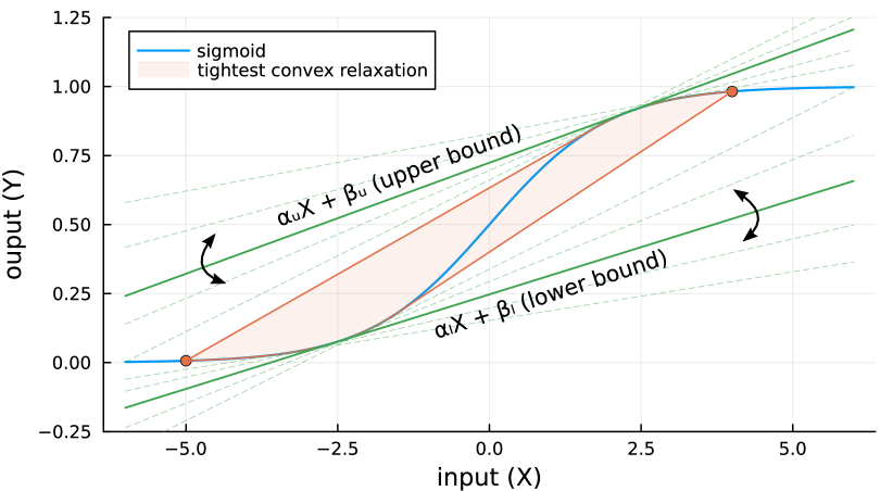
In (6), the terms are negative for the upper bounds, and positive for the lower bounds, as stated in the appendix. Associated affine bounds are plotted in Fig. 2. As depicted, these bounds are capable of yielding the tightest possible convex relaxation of the sigmoid activation function. Denoting (6) by , we define a set of valid values:
| (7) |
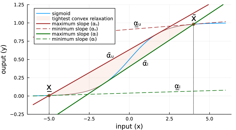
The minimum and maximum allowable slope values, and , are predetermined for every sigmoid activation function. Nominally, , since , and , since . However, tighter slopes generally exist, based on the sigmoid’s minimum and maximum input bounds and . Fig. 3 illustrates a typical situation, where there are distinct slope bounds. In this figure, the minimum slopes (dashed lines) are simply computed as the gradients at the minimum and maximum inputs:
| (8) | ||||
| (9) |
The maximum bounding slopes and , however, are computed as the lines which intersect the sigmoid at two points: the bounded input anchor points ( and ), and a corresponding tangent point. The parallelized calculation of these slopes is a pre-processing step involving sequential quadratic formulate iterations, and the associated procedures are discussed in the appendix.
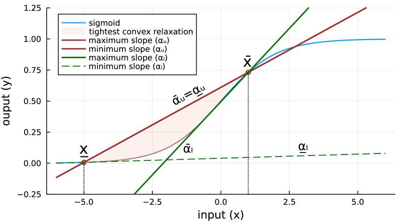
Fig. 4 illustrates an alternative situation, where the maximum and minimum affine upper bound slopes are equal111Depending on the values of and , this can also happen to the affine lower bounds: . However, due to the nonlinearity of the sigmoid, and cannot occur simultaneously, unless , which is a degenerate case.: . This occurs when the tangent slope at can be “raised up” such that the corresponding affine bound eventually intersects with . Defining , we have two possibilities:
| (10a) | ||||
| (10b) | ||||
Similarly, in the lower affine bound case,
| (11a) | ||||
| (11b) | ||||
In either case, equal slopes can be directly computed as
| (12) |
Backward Bound Propagation
To efficiently minimize , as in (3), we utilize the backward bound propagation procedure employed in, e.g., (Wang et al. 2021). In applying this procedure, however, we utilize a sequential backward evaluation step in order to dynamically detect if a sigmoid function should be upper, or lower, bounded by the affine bound in (6). Consider, for example, the simple problem
| (13) |
where is some cost vector. To achieve minimum cost,
-
•
if , then should lower bound the sigmoid;
-
•
if , then should upper bound the sigmoid.
This procedure is sequentially applied as we move backward through the NN layers. The coefficients in front of each layer, however, will be a function of the numerical values, which will be changing at each gradient step during the verification solve. In the appendix, we define a NN mapping (20), and then we sequentially move backward through this mapping in (21), inferring the sign of the coefficients in front of each affine bound term.
Dual Verification
Using the affine relaxed version of the NN mapping in (20), we may start with input to sequentially replace all intermediate primal variables:
| (14a) | ||||
| (14b) | ||||
The associated minimization problem over this relaxed verification problem is given by
| (15a) | ||||
| (15b) | ||||
where the dual norm (Wang et al. 2021; Chevalier, Murzakhanov, and Chatzivasileiadis 2024) has been used to transform the norm constraint into a norm objective term. Any valid (i.e., feasible) set of , parameters will yield a valid lower bound for the relaxed verification problem. To achieve the tightest lower bound, we may maximize over the feasible set of , :
| (16) |
While are not dual variables in the traditional sense, they are responsible for actively constraining the primal space, so we we refer to (16) as a dual problem.
While (16) can be solved via projected gradient ascent, we may alternatively use in order to eliminate the variable entirely. Initial testing shows that eliminating , and then backpropagating through , is more effective than equality projecting feasible, via (6), at each step. The updated formulation is given via
| (17) |
Projected gradient-based solution routine
We use a projected gradient routine in order to solve (17) and enforce . Sigmoid functions may need to be upper bounded via (29), and then lower bounded via (30), as numerical values of evolve. To overcome this challenge, at each step of our numerical routine, we reverse propagate compute the sign vector , from (21), for each layer. Since this vector tells us if the sigmoid function should be upper or lower bounded, we embed corresponding elements of this vector inside of (6), replacing the terms. At the activation function of each NN layer, the corresponding slope and sign elements are feasibly related via
| (18) |
With this parameterization embedded inside of (17), we backpropagate through the objective function and take a gradient step with . Next, we clip all values of to remain between and , depending on whether the corresponding is acting like an upper or lower affine bound. The full gradient-based verification routine for a sigmoid-based NN is given in Alg 1, which we refer to as -sig. The bounds , for each activation function are treated as inputs.
Input: , for each activation function
Output: : solution to (17)
Test Results
In order to test the effectiveness of -sig and Alg. 1, we optimized over a range of randomly generated sigmoid-based NNs in two separate experiments. All NNs consisted of four dense layers with sigmoid activation functions, followed by a dense linear layer. We considered NNs containing 5, 10, 50, 100, 500, and 1000 neurons per layer. For each NN size, we generated and verified over 5 independent NN instantiations. The posed verification problem sought to minimize the sum of all outputs (i.e., the vector from (20a) was set to the vector of all ones), and we assumed an allowable infinity norm perturbation of (i.e., ). To generate initial loose activation function bounds for all NN layers, we applied vanilla interval bound propagation via (39), as reviewed in the appendix. We note that tighter bounds could potentially be achieved via IBP + backward mode LiRPA (Xu et al. 2020), but we chose to utilize weaker IBP-based bounds to initialize -sig in order to highlight its effectiveness without strong initial activation function bounds.
In each test, we took 300 projected gradient steps in pursuit of solving (17). We then benchmarked our results against -CROWN + auto-LiRPA (Xu et al. 2021, 2020). In order to fairly compare, we increased the default -CROWN iteration count by 3-fold, to 300 iterations. To avoid an early exit from CROWN (i.e., due to a successfully proved bound), we set the VNN-LIB (Ferrari et al. 2022) verification metric to an arbitrarily high value (i.e., prove ). In order to compare the bounds proved via our -sig in Alg. 1 vs -CROWN, we defined :
| (19) |
where represents the percent improvement or decline of our bound relative to -CROWN (positive means -sig provides a tighter bound than -CROWN, while negative means the bound in looser). -sig was built in Julia, and all code is provided as supplementary material.
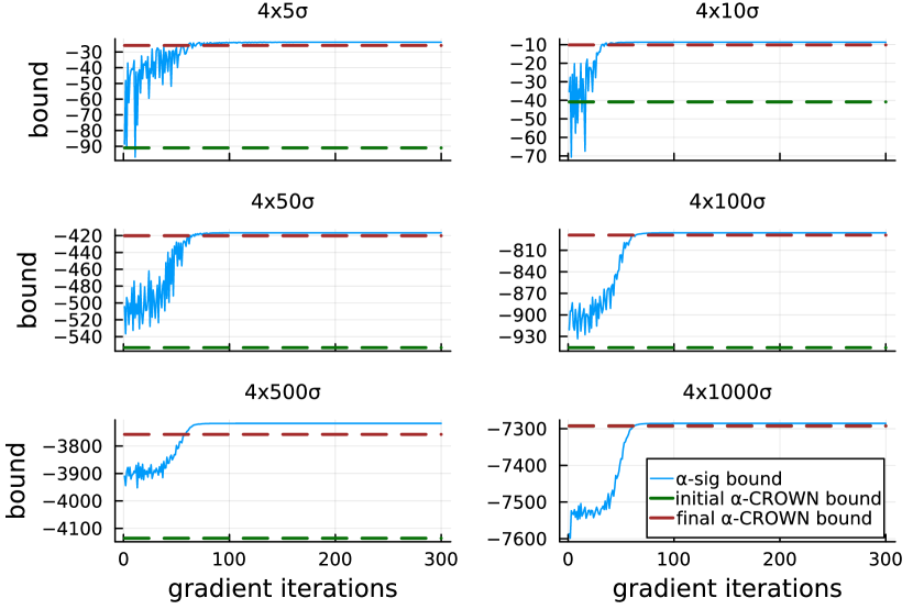
Experiment 1: Varying weight distributions. Normally distributed weight and bias parameters tend to yield NNs whose sigmoid activation functions are always stuck on or off. In order to avoid this, we we initialized all NN weights and biases via and , where represents the model index; thus, in this experiment, the weight parameter variances for each NN model progressively shrank (for a given model size). Results associated with this test are given in Table 1: in this table, the values through represent bound comparisons, à la (19), across five independently generated models (five for each NN size). Clearly, -sig tended to provide marginally tighter bounds than -CROWN. Across all six NN sizes, the bound progressions for -sig are illustrated in Fig. 5. In this figure, initial CROWN and fully optimized -CROWN bounds are superimposed for reference.
In the upper-right portion of Table 1, -CROWN outperformed -sig. The reason why is apparent and interesting: in our experiments, -sig was initialized with fairly loose IBP-based primal bounds , (see input to Alg. 1). As NN models shrink in size and weight parameter variances drop, auto-LiRPA’s proclivity for primal bound solving seems to overtake -sig’s optimal tightening of the sigmoid activation function. The benefit of -sig, however, is also in its speed. As demonstrated in Table 2, -sig can be up to two orders of magnitude faster222One of the trial times was removed due to CROWN error: “Pre-activation bounds are too loose for BoundSigmoid”. than -CROWN, while still yielding better bounds in many cases.
| NN Size | |||||
|---|---|---|---|---|---|
| +8.02 | -18.9 | -6.1 | -21.2 | -31.8 | |
| +14.6 | -7.23 | -28.1 | -26.4 | -24.0 | |
| +0.83 | +0.51 | +0.23 | -4.25 | -9.63 | |
| +0.40 | +0.34 | +0.04 | -0.52 | -1.60 | |
| +1.06 | +0.13 | +0.14 | +0.10 | +0.03 | |
| +0.09 | +0.81 | +0.11 | +0.11 | +0.06 |
| NN Size | -CROWN | -sig | -sig speedup |
|---|---|---|---|
| 37.41 sec | 0.10 sec | 360.4x | |
| 37.77 sec | 0.105 sec | 358.4x | |
| 38.33 sec | 0.17 sec | 223.1x | |
| 37.90 sec | 0.40 sec | 95.1x | |
| 53.42 sec | 2.65 sec | 20.2x | |
| 82.90 sec | 9.98 sec | 8.3x |
Experiment 2: Consistent weight distributions. In this test, we initialized all NN weights and biases with consistent distributions: and . Results from across five randomly initialized models are shown in Table 3. In contrast to the first experiment, -sig was able to reliably outperform -CROWN. In this case, the larger weight parameter variances seemed to cause inherently looser primal bounds, meaning -CROWN’s advantage over -sig was lessened.
| NN Size | |||||
|---|---|---|---|---|---|
| -7.30 | +17.9 | -32.99 | -8.12 | -0.37 | |
| +4.6 | +28.1 | -1.31 | +2.29 | -2.66 | |
| +1.26 | +0.49 | +0.64 | +1.21 | +0.95 | |
| +0.47 | +0.51 | +0.65 | +0.70 | +0.57 | |
| +0.99 | +0.98 | +1.02 | +0.97 | +0.98 | |
| +0.13 | +0.19 | +0.09 | +0.12 | +0.12 |
Discussion and Conclusion
Verifying over NNs containing S-shaped activation functions is inherently challenging. In this paper, we presented an explicit, differentiable mapping between the slope and y-intercept of an affine expression which tangentially bounds a sigmoid function. By optimizing over this bound’s parameters in the dual space, our proposed convex relaxation of the sigmoid is maximally tight (i.e., a tighter element-wise relaxation of the sigmoid activation function does not exist). As explored in the test results section, however, our ability to fully exploit this tightness hinges on having good primal bounds , for all activation functions. For example, given the bounds , , our approach collapses to a useless box constraint.
Even with relatively loose IBP-based activation function bounds, however, our proposed verification routine “-sig” is able to () marginally outperform -CROWN in terms of bound tightness, and () substantially outperform it in terms of computational efficiency. Future work will attempt to marry LiRPA/CROWN’s excellent proclivity for activation function bounding with -sig’s element-wise activation function tightening prowess. Future work will also extend the approach presented in this paper to other S-shaped activation functions, along with the multi-variate softmax function.
Appendix A APPENDICES
Appendix B Neural Network Mapping and Relaxation
The NN mapping, whose output is transformed by a verification metric , is stated below. At each sigmoid activation function, we also state the corresponding affine relaxation, where diagonalizes an vector into a diagonal matrix:
| (20a) | ||||
| (20b) | ||||
| (20c) | ||||
| (20d) | ||||
| (20e) | ||||
| (20f) | ||||
| (20g) | ||||
| (20h) | ||||
We may now relax the sigmoid activation functions, replacing them with their affine bounds. To determine if each scalar , pair are chosen to be an upper bound or a lower bound, we need to determine the coefficient in front of the corresponding activation function. To do this, we move backward through the NN, defining vectors of sign values corresponding to the signs of the entries in the argument:
| (21a) | ||||
| (21b) | ||||
| (21c) | ||||
| (21d) | ||||
Appendix C Slope and Intercept Relation Derivation
Starting from (5b), the sigmoid derivative can be written via . Setting this equal to the upper affine bound slope, we have
| (22a) | ||||
| (22b) | ||||
Multiplying through by the expanded right-side denominator, we may solve for the primal variable explicitly:
| (23) | ||||
| (24) | ||||
| (25) | ||||
| (26) |
Since , the solution for is non-unique, which is an inherent consequence of the symmetry of the sigmoid function, where exactly two points in the sigmoid manifold will map to the same slope. Notably, however, the affine upper bound will map to positive solutions of , i.e., in the region where the sigmoid function is concave, and the affine lower bound will map to negative values of , i.e., in the region where the sigmoid function is convex:
| (27) | ||||
| (28) |
Reorganizing the intersection equation (5a), such that , we may plug the primal solutions (27)-(28) in for . This yields explicit expressions for the intercept points (, ) as functions of the slopes (, ):
| (29) | ||||
| (30) |
Appendix D Computing Maximum Slope Limits
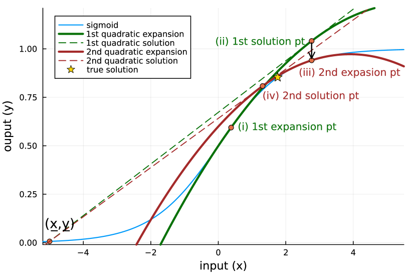
In order to compute the maximum slope values and , as depicted in Fig. 3, we use a sequential numerical routine which iteratively solves a quadratic expansion of the associated problem. Consider the following system of equations, with unknown variables , , and (intercept point):
| anchor point | (31) | ||||
| (32) | |||||
| (33) |
where the known “anchor point” is depicted in Fig. 6. Despite its similarity to (5), this system does not have a closed-form solution (i.e., it will result in a single nonlinear equation, similar to (6), but with replaced by an expression for ). In order to efficiently solve this system of equations, we perform a single quadratic expansion of the sigmoid activation function (Agarwal et al. 2022):
| (34) |
where , etc., is used for notational simplicity. Collecting like powers of , the quadratic expansion yields
The updated system of equations is now quadratic:
| anchor point | (35) | ||||
| approx intersection | (36) | ||||
| (37) |
In this system, we may eliminate the and terms by setting and , which yields . Plugging these into (36), a single quadratic equation emerges:
We reorganize these terms into a standard quadratic form:
| (38) |
where coefficients , , are written as functions of the expansion point . We use the quadratic formula to analytically solve (38). Multiple iterations of () updating the coefficients and then () re-solving (38) via quadratic formula yields rapidly converging solutions to the original system (31)-(33). Due to the analytical exactness of the quadratic formula, this routine converges faster than Newton iterations at a similar computational expense. Two iterations of this routine are depicted in Fig. 6, where the second solution falls very close to the true solution (which future iterations converge to). Once the solution is found, we recover via . The procedure is applied to find the maximum upper affine bound slope in Fig. 6; an identical procedure is applied to find the maximum lower affine bound slope.
Appendix E Interval Bound Propagation
Appendix F Acknowledgments
References
- Agarwal et al. (2022) Agarwal, A.; Pandey, A.; Bandele, N. T.; and Pileggi, L. 2022. Generalized Smooth Functions for Modeling Steady-State Response of Controls in Transmission and Distribution. Electric Power Systems Research, 213: 108657.
- Brix et al. (2023a) Brix, C.; Bak, S.; Liu, C.; and Johnson, T. T. 2023a. The Fourth International Verification of Neural Networks Competition (VNN-COMP 2023): Summary and Results. arXiv:2312.16760.
- Brix et al. (2023b) Brix, C.; Müller, M. N.; Bak, S.; Johnson, T. T.; and Liu, C. 2023b. First Three Years of the International Verification of Neural Networks Competition (VNN-COMP). arXiv:2301.05815.
- Bunel et al. (2020) Bunel, R.; Hinder, O.; Bhojanapalli, S.; Krishnamurthy; and Dvijotham. 2020. An efficient nonconvex reformulation of stagewise convex optimization problems. arXiv:2010.14322.
- Chevalier and Chatzivasileiadis (2024) Chevalier, S.; and Chatzivasileiadis, S. 2024. Global Performance Guarantees for Neural Network Models of AC Power Flow. arXiv:2211.07125.
- Chevalier, Murzakhanov, and Chatzivasileiadis (2024) Chevalier, S.; Murzakhanov, I.; and Chatzivasileiadis, S. 2024. GPU-Accelerated Verification of Machine Learning Models for Power Systems. Hawaii International Conference on System Sciences.
- Everett (2021) Everett, M. 2021. Neural network verification in control. In 2021 60th IEEE Conference on Decision and Control (CDC), 6326–6340. IEEE.
- Ferrari et al. (2022) Ferrari, C.; Muller, M. N.; Jovanovic, N.; and Vechev, M. 2022. Complete verification via multi-neuron relaxation guided branch-and-bound. arXiv preprint arXiv:2205.00263.
- Gowal et al. (2019) Gowal, S.; Dvijotham, K.; Stanforth, R.; Bunel, R.; Qin, C.; Uesato, J.; Arandjelovic, R.; Mann, T.; and Kohli, P. 2019. On the Effectiveness of Interval Bound Propagation for Training Verifiably Robust Models. arXiv:1810.12715.
- Henriksen and Lomuscio (2020) Henriksen, P.; and Lomuscio, A. 2020. Efficient neural network verification via adaptive refinement and adversarial search. In ECAI 2020, 2513–2520. IOS Press.
- Ildiz et al. (2024) Ildiz, M. E.; Huang, Y.; Li, Y.; Rawat, A. S.; and Oymak, S. 2024. From Self-Attention to Markov Models: Unveiling the Dynamics of Generative Transformers. arXiv:2402.13512.
- Lyu et al. (2019) Lyu, Z.; Ko, C.-Y.; Kong, Z.; Wong, N.; Lin, D.; and Daniel, L. 2019. Fastened CROWN: Tightened Neural Network Robustness Certificates. arXiv:1912.00574.
- Salman et al. (2020) Salman, H.; Yang, G.; Zhang, H.; Hsieh, C.-J.; and Zhang, P. 2020. A Convex Relaxation Barrier to Tight Robustness Verification of Neural Networks. arXiv:1902.08722.
- Shi et al. (2024) Shi, Z.; Jin, Q.; Kolter, Z.; Jana, S.; Hsieh, C.-J.; and Zhang, H. 2024. Neural Network Verification with Branch-and-Bound for General Nonlinearities. arXiv:2405.21063.
- Singh et al. (2019) Singh, G.; Gehr, T.; Püschel, M.; and Vechev, M. 2019. An abstract domain for certifying neural networks. Proceedings of the ACM on Programming Languages, 3(POPL): 1–30.
- Sun et al. (2024) Sun, L.; Huang, Y.; Wang, H.; Wu, S.; Zhang, Q.; Li, Y.; Gao, C.; Huang, Y.; Lyu, W.; Zhang, Y.; Li, X.; Liu, Z.; Liu, Y.; Wang, Y.; Zhang, Z.; Vidgen, B.; Kailkhura, B.; Xiong, C.; Xiao, C.; Li, C.; Xing, E.; Huang, F.; Liu, H.; Ji, H.; Wang, H.; Zhang, H.; Yao, H.; Kellis, M.; Zitnik, M.; Jiang, M.; Bansal, M.; Zou, J.; Pei, J.; Liu, J.; Gao, J.; Han, J.; Zhao, J.; Tang, J.; Wang, J.; Vanschoren, J.; Mitchell, J.; Shu, K.; Xu, K.; Chang, K.-W.; He, L.; Huang, L.; Backes, M.; Gong, N. Z.; Yu, P. S.; Chen, P.-Y.; Gu, Q.; Xu, R.; Ying, R.; Ji, S.; Jana, S.; Chen, T.; Liu, T.; Zhou, T.; Wang, W.; Li, X.; Zhang, X.; Wang, X.; Xie, X.; Chen, X.; Wang, X.; Liu, Y.; Ye, Y.; Cao, Y.; Chen, Y.; and Zhao, Y. 2024. TrustLLM: Trustworthiness in Large Language Models. arXiv:2401.05561.
- Trinh et al. (2024) Trinh, T. H.; Wu, Y.; Le, Q. V.; He, H.; and Luong, T. 2024. Solving olympiad geometry without human demonstrations. Nature, 625(7995): 476–482.
- Urban and Miné (2021) Urban, C.; and Miné, A. 2021. A Review of Formal Methods applied to Machine Learning. arXiv:2104.02466.
- Wang et al. (2021) Wang, S.; Zhang, H.; Xu, K.; Lin, X.; Jana, S.; Hsieh, C.-J.; and Kolter, J. Z. 2021. Beta-crown: Efficient bound propagation with per-neuron split constraints for neural network robustness verification. Advances in Neural Information Processing Systems, 34: 29909–29921.
- Wei et al. (2023) Wei, D.; Wu, H.; Wu, M.; Chen, P.-Y.; Barrett, C.; and Farchi, E. 2023. Convex Bounds on the Softmax Function with Applications to Robustness Verification. arXiv:2303.01713.
- Wu et al. (2023) Wu, H.; Tagomori, T.; Robey, A.; Yang, F.; Matni, N.; Pappas, G.; Hassani, H.; Pasareanu, C.; and Barrett, C. 2023. Toward Certified Robustness Against Real-World Distribution Shifts. In 2023 IEEE Conference on Secure and Trustworthy Machine Learning (SaTML), 537–553.
- Wu and Zhang (2021) Wu, Y.; and Zhang, M. 2021. Tightening Robustness Verification of Convolutional Neural Networks with Fine-Grained Linear Approximation. Proceedings of the AAAI Conference on Artificial Intelligence, 35(13): 11674–11681.
- Xu et al. (2020) Xu, K.; Shi, Z.; Zhang, H.; Wang, Y.; Chang, K.-W.; Huang, M.; Kailkhura, B.; Lin, X.; and Hsieh, C.-J. 2020. Automatic Perturbation Analysis for Scalable Certified Robustness and Beyond. arXiv:2002.12920.
- Xu et al. (2021) Xu, K.; Zhang, H.; Wang, S.; Wang, Y.; Jana, S.; Lin, X.; and Hsieh, C.-J. 2021. Fast and Complete: Enabling Complete Neural Network Verification with Rapid and Massively Parallel Incomplete Verifiers. In International Conference on Learning Representations.
- Zhang et al. (2022a) Zhang, H.; Wang, S.; Xu, K.; Wang, Y.; Jana, S.; Hsieh, C.-J.; and Kolter, Z. 2022a. A Branch and Bound Framework for Stronger Adversarial Attacks of ReLU Networks. In Chaudhuri, K.; Jegelka, S.; Song, L.; Szepesvari, C.; Niu, G.; and Sabato, S., eds., Proceedings of the 39th International Conference on Machine Learning, volume 162 of Proceedings of Machine Learning Research, 26591–26604. PMLR.
- Zhang et al. (2022b) Zhang, Z.; Wu, Y.; Liu, S.; Liu, J.; and Zhang, M. 2022b. Provably Tightest Linear Approximation for Robustness Verification of Sigmoid-like Neural Networks. arXiv:2208.09872.