On a fundamental difference between Bayesian and frequentist approaches to robustness

Abstract

Heavy-tailed models are often used as a way to gain robustness against outliers in Bayesian analyses. On the other side, in frequentist analyses, M-estimators are often employed. In this paper, the two approaches are reconciled by considering M-estimators as maximum likelihood estimators of heavy-tailed models. We realize that, even from this perspective, there is a fundamental difference in that frequentists do not require these heavy-tailed models to be proper. It is shown what the difference between improper and proper heavy-tailed models can be in terms of estimation results through two real-data analyses based on linear regression. The findings of this paper make us ponder on the use of improper heavy-tailed data models in Bayesian analyses, an approach which is seen to fit within the generalized Bayesian framework of Bissiri et al. (2016) when combined with proper prior distributions yielding proper (generalized) posterior distributions.

¹Department of Mathematics and Statistics, Université de Montréal.

²Department of Mathematics, Université du Québec à Montréal.

Keywords: heavy-tailed distributions, M-estimators, outliers, regression.

1 Introduction

Let us assume that we have access to a data set of the form $\{\mathbf{x}_{i},y_{i}\}_{i=1}^{n}$, where $\mathbf{x}_{1},\ldots,\mathbf{x}_{n}\in\operatorname{\mathbb{R}}^{p}$ are $n\in\operatorname{\mathbb{N}}$ vectors of explanatory-variable data points and $y_{1},\ldots,y_{n}\in\operatorname{\mathbb{R}}$ are $n$ observations of a dependent variable, $p$ being a positive integer. Let us assume that one is interested in modelling the dependent variable through its relationship with the explanatory variables, and therefore in using a regression model.

It is often the case that the data set used for model estimation is contaminated by outliers (i.e., erroneous or extreme data points). Suppose that there exists a trend in the bulk of the data (i.e., the non-outliers), and that the model is used to capture this trend. We define an outlier as a couple $(\mathbf{x}_{i},y_{i})$ whose components are incompatible with this trend. It is thus not necessary that either component, $\mathbf{x}_{i}$ or $y_{i}$, be extreme (in the sense of being large in norm); rather, it is the combination of this $\mathbf{x}_{i}$ with that $y_{i}$ that makes the couple an outlier.

Typical regression models are not robust against outliers, meaning that a difference in trends in the bulk of the data and the outliers yields skewed inference and predictions. A canonical example of such non-robust models is a linear regression with normal errors for which maximum likelihood estimation of the regression coefficients corresponds to ordinary least squares (OLS). Often, Bayesians identify the cause of the robustness problem by analysing the model and directly adapt the latter to the potential presence of outliers. With normal linear regression, the cause of the problem is the exponential decay of the tails which creates a conflict between the outliers and the model (O’Hagan and Pericchi, 2012). Instead, a Student’s $t$ distribution is often assumed given that its heavier tails (partially) resolve this conflict by increasing the likelihood of outliers (West, 1984; Gagnon and Hayashi, 2023). A reason why the Student’s $t$ distribution is the preferred heavy-tailed alternative to the normal is that the densities are similar, except for the tail decay. This implies that in the absence of outliers, the Student’s $t$ model leads to inference similar to that with the normal model, which is a desirable property often referred to as efficiency in a robustness context. Ideally, robust approaches act automatically as practitioners would and exclude outliers when they are far enough apart and there is no doubt as to whether they really are outliers (West, 1984). An approach that has this property is said to be wholly robust. Such an approach, together with a density similar to the normal (except for the tail decay), imply that the robust model leads to similar estimation results as with the normal when the outliers are far enough, but where the estimation of the normal model in this case is based on the data set without the outliers. Another feature of the best robust approaches — those that demonstrate both efficiency and whole robustness — is their ability to gradually diminish the impact of observations when artificially moved away from the bulk of the data. This feature allows for a certain influence of moderately far observations, reflecting uncertainty about the nature of these observations in a grey zone (outliers versus non-outliers).

Throughout the years it has been found that, even tough heavy, the tails of the Student’s $t$ probability density function (PDF) are not heavy enough to reach whole robustness in the context of linear regression (Gagnon and Hayashi, 2023). The log-Pareto-tailed normal (LPTN), a PDF introduced in Desgagné (2015), has been shown to have sufficiently heavy tails to achieve whole robustness (Gagnon et al., 2020). The central part of this continuous PDF coincides with that of the standard normal and the tails are log-Pareto, meaning that they behave like $(1/|z|)(1/\log|z|)^{\lambda}$ with $\lambda>1$, hence its name. The LPTN PDF belongs to a family of PDFs introduced in Desgagné (2015) which are referred to as log-regularly varying. The level of tail heaviness is somewhat extreme because the tails are heavier than any Student’s $t$ distribution (with any degrees of freedom), and if we were to set $\lambda=1$, which can be seen as a way to gain further in tail heaviness, we would obtain a density function which is not integrable and thus improper.

On the frequentist side, instead of directly modifying the model to gain robustness, robust estimators are often derived through a modification of the log-likelihood function or its derivative. In the context of normal linear regression for instance, the source of the robustness problem is identified as the quadratic function applied to the residuals in the log-likelihood function which significantly increases the impact of outliers. This quadratic function is replaced by one that grows less rapidly. When the modification is regarding the log-likelihood function, the approach yields what is referred to as an M-estimator (Huber, 1964).

The rationale behind both frequentist and Bayesian approaches is the same, and in some cases there exists a perfect connection between the approaches (Gagnon and Wang, 2024). For instance, in linear regression, the Huber M-estimator (Huber, 1973) can be seen as the maximum likelihood estimator of a model where the PDF of the errors has tails with the same decay as those of the Laplace PDF; thus the tails are heavier than those of the normal PDF. There is, however, a fundamental difference between the frequentist and Bayesian approaches to robustness. On one side, the modified log-likelihood function (in the context of M-estimation) is not required to correspond to a proper model. For instance, Tukey’s biweight M-estimator (Beaton and Tukey, 1974) does not correspond to a proper model as the modified log-likelihood function is constant beyond a threshold, thus yielding an improper distribution. On the other side, Bayesians (typically) require the model to be proper and are thus limited in tail heaviness of the PDF they use. In this paper, we demonstrate that this fundamental difference between the frequentist and Bayesian approaches may lead to significantly different estimation results, where the Bayesian results are more influenced by the presence of outliers, even when using the super heavy-tailed LPTN PDF. We focus on linear regression for explanations and examples, but it is clear that the aforementioned fundamental difference between the frequentist and Bayesian approaches to robustness exists and has consequences beyond the context of linear regression.

The findings of this paper make us realize that a way to further reconcile the Bayesian and frequentist approaches would be to accept the use of improper heavy-tailed data models in Bayesian analyses, while using in return proper prior distributions in order to obtain proper posterior distributions. This fits within the generalized Bayesian framework of Bissiri et al. (2016) under which it is acknowledged that models like linear regression are plausibly misspecified; the likelihood function is thus replaced by a loss function in a (generalized) posterior distribution. If one does not find the use of improper data models acceptable, then one could question the use of M-estimators such as Tukey’s biweight.

The classic frequentist robust approaches in the context of linear regression are arguably those mentioned above, namely the Huber and Tukey’s biweight M-estimators. On the Bayesian side, the Student’s $t$ model is the classic approach. We present results for the LPTN model which is seen as similar to the Student’s $t$ model, but with heavier tails. We evaluate a spectrum of tail decay by trying different values for $\lambda$, and in particular, values close to 1, representing the properness limit of the LPTN model. When the M-estimators are considered as maximum likelihood estimators of (possibly improper) heavy-tailed models, the four approaches just mentioned all fall under the same category: heavy-tailed alternatives to the standard normal. The main difference is in the tail decay, from exponential to an absence of decay which is the most extreme type. The focus in this paper is on this classic category of approaches to robustness.

In Figure 1, we present a first example of difference between Bayesian and frequentist robust estimation. In Figure 1 (a), we show estimation results for the simple linear regression, based on the shock data set accessible via the R package RobStatTM. This data set is about an experiment conducted on rats to evaluate the average time to go through a shuttlebox depending on the number of electric shocks dispensed. Visually, we observe that Tukey’s biweight M-estimation offers a better fit, in the sense that the line passes through the majority of the data points (which can be considered as the non-outliers); OLS estimation and Bayesian LPTN model estimation are quite influenced by the outliers. In this example, the level of outlier contamination is severe for the ratio of the number of data points to the number of unknown parameters. Even though the LPTN model has the whole robustness property, the latter is an asymptotic property. Therefore, when outliers are far, but not extremely far, there can be a significant difference between the posterior distribution that excludes the outliers and the one that does not. In such a situation, Tukey’s biweight M-estimator may be less influenced by the outliers due to the shape of its modified log-likelihood function. The influence of the outliers or any data point can be deduced from the assigned weight in the estimation; a formal definition of the weight function is given in Section 2. In Figure 1 (b), we present the weight assigned to each data point by Tukey’s biweight M-estimator and the Bayesian LPTN one. Note that the OLS estimator assigns a weight of 1 to all the data points.

$\begin{array}[]{cc}\includegraphics[width=216.81pt]{Fig_scatter_ex_1.pdf}&\includegraphics[width=216.81pt]{Fig_weights_ex_1.pdf}\cr\textbf{(a) }&\textbf{(b)}\end{array}$

Figure 1: (a) Estimation of a simple linear regression based on the shock data set using OLS and Tukey’s biweight M-estimator, as well as the maximum a posteriori estimate of a Bayesian LPTN model. (b) Weight assigned to each data point by Tukey’s biweight M-estimator and the Bayesian LPTN one.

We now present how the rest of the paper is organized. In Section 2, we provide an overview of M-estimators and Bayesian heavy-tailed models, which will allow to make more precise what have been discussed above. In particular, we present M-estimators as maximum likelihood estimators of (possibly improper) heavy-tailed models. Also, we explain how improper heavy-tailed data models could be used in (generalized) Bayesian analyses and how they could yield estimation results such as those obtained with Tukey’s biweight M-estimator. In Section 3, we show that the example about the shock data set above is not unique. We provide another real-data example where the same phenomenon as in Figure 1 is observed. This time the model is more complex as the number of covariates is larger, but the situation is similar in the sense that the outlier contamination is again severe for the ratio of the number of data points to the number of unknown parameters.

Note that in the example of the shock data set, Student’s $t$ models with degrees of freedom around 1 allow to obtain similar estimation results to Tukey’s biweight M-estimator. This is somewhat unexpected as the Student’s $t$ PDF as a faster tail decay than the LPTN PDF. In the example of Section 3, it is however not the case and the estimation results with the LPTN model are less influenced by the presence of outliers (yet, the influence is significant, again contrarily as with Tukey’s biweight M-estimator). Between the Student’s $t$ and LPTN models, the difference in tail decay can be seen as being slight, but there is also a slight difference in density shape. The LPTN PDF exactly matching the standard normal on the central part, it decreases faster than the standard normal for a short interval at the beginning of the tails after which it goes above, a consequence of the continuity of the LPTN density with a constraint of integrating to 1. The Student’s $t$ model is constructed otherwise with a density that becomes flatter when decreasing the degrees of freedom. The insensitivity of the estimation results with Student’s $t$ models in the example of the shock data set made us realize that, if we could slightly flatten the LPTN PDF, we may end up with insensitivity in this example with this model as well. We managed to achieve this by going beyond the constraint $\lambda>1$ and setting $\lambda=1$ but changing nothing else in the model, thus yielding an improper density.

2 Overview of frequentist and Bayesian robust approaches

2.1 M-estimators

In linear regression, it is assumed that $y_{1},\ldots,y_{n}$ are realizations of $n$ random variables $Y_{1},\ldots,Y_{n}$ defined through the following model:

$$Y_{i}=\mathbf{x}_{i}^{T}\bm{\beta}+\sigma\varepsilon_{i},\quad i=1,\ldots,n,$$ (1)

where $\bm{\beta}:=(\beta_{1},\ldots,\beta_{p})^{T}\in\operatorname{\mathbb{R}}^{p}$ is a vector of regression coefficients, $\sigma>0$ is a scale parameter and $\varepsilon_{1},\ldots,\varepsilon_{n}\in\operatorname{\mathbb{R}}$ are standardized errors. In an homoscedastic model, it is assumed that $\varepsilon_{1},\ldots,\varepsilon_{n}$ are independent and identically distributed (IID) random variables, each having a PDF denoted by $f$.

The log-likelihood function is given by

$$\ell(\bm{\beta},\sigma):=-n\log\sigma+\sum_{i=1}^{n}\log f\left(\frac{y_{i}-\mathbf{x}_{i}^{T}\bm{\beta}}{\sigma}\right).$$ (2)

When $f$ is a standard normal PDF, we have $f(\varepsilon)=g(\varepsilon)/m$ with $g(\varepsilon)=\exp(-\epsilon^{2}/2)$ and $m=\sqrt{2\pi}$, the normalizing constant. The quadratic term resulting from $-\log g$ produces particularly extreme values when some residuals $y_{i}-\mathbf{x}_{i}^{T}\bm{\beta}$ are extreme, which is the case for outliers when the log-likelihood function is evaluated at parameter values reflecting the trend in the bulk of the data. To alleviate the impact and thus the sensitivity to outliers, the quadratic function is replaced in M-estimation. We can view this approach as replacing the function $g$. From the new function $g$, we can identify a log-likelihood function as in (2) and consider M-estimation as maximum likelihood estimation of the model in (1), but with this new function $g$. When this function is integrable, $g$ is equivalent to a PDF $f$, up to a normalizing constant $m$. When it is not integrable and $m$ is thus not well defined, we will still consider that (1) with this function $g$ is a model, but an improper one. Note that, from an M-estimation perspective, this is not a problem as the estimation procedure corresponds to the maximization of (2) with $m$ omitted.

The Huber M-estimator results from setting

$$-\log g(\varepsilon)=\left\{\begin{array}[]{lcc}\varepsilon^{2}/2&\text{ if }&|\varepsilon|\leq k,\cr k|\varepsilon|-k^{2}/2&\text{ if }&|\varepsilon|>k,\cr\end{array}\right.$$

with $k$ a tuning parameter controlling the tradeoff between robustness and efficiency. M-estimation in this case can thus be viewed as maximum likelihood estimation of the model in (1) with $f$ as follows:

$$f(\varepsilon)=\frac{g(\varepsilon)}{m}=\left\{\begin{array}[]{lcc}\exp(-\varepsilon^{2}/2)/m&\text{ if }&|\varepsilon|\leq k,\cr\exp(-k|\varepsilon|-k^{2}/2)/m&\text{ if }&|\varepsilon|>k,\cr\end{array}\right.$$

where $m=2\mathrm{e}^{-k^{2}/2}/k+\sqrt{2\pi}(2\Phi(k)-1)$, $\Phi$ being the cumulative distribution function of a standard normal. An advantage of Huber M-estimation is that the resulting function $\ell$ (with the same form as in (2)) is concave and smooth, like with the normal errors, which is a desirable property for optimization purposes. A disadvantage is that the growth of $-\log g$ is still rapid, implying sensitivity to outliers.

Tukey’s biweight M-estimator comes with a gain on one side, but a loss on the other. It results from setting

$$-\log g(\varepsilon)=\left\{\begin{array}[]{lcc}1-(1-(\varepsilon/k)^{2})^{3}&\text{ if }&|\varepsilon|\leq k,\cr 1&\text{ if }&|\varepsilon|>k,\cr\end{array}\right.$$ (5)

where we used the same notation $k$ as with the Huber M-estimator given that this tuning parameter plays the same role here. The function $-\log g$ in (5) has appealing properties. It is similar to the quadratic function on the central part (but it operates on a different scale), while being constant on the extremities and being smooth; see Section A.2 for a figure. However, the resulting function $\ell$ is not concave.

The fact that it is constant on the extremities implies that $m$ is not well defined in this case as $g$ is not integrable. With the function $g$ in (5), $g(\varepsilon)=\exp(-1)$ whenever $|\varepsilon|>k$, implying that this density assigns the same measure $\int_{I}g(\varepsilon)\,\mathrm{d}\varepsilon$ to all intervals $I$ of same length, regardless of the distance to the origin, as long as the condition $|\varepsilon|>k$ is satisfied for all points in the intervals. Viewing probability distributions as measures, this characteristic of Tukey’s biweight M-estimator allows to gain understanding regarding its behaviour, even if it is associated to an improper model. Regarding now the function to optimize, with a similar form as in (2), we have that

$$g\left(\frac{y_{i}-\mathbf{x}_{i}^{T}\bm{\beta}}{\sigma}\right)=\exp(-1),$$

when $|y_{i}-\mathbf{x}_{i}^{T}\bm{\beta}|/\sigma>k$. Therefore, $g((y_{i}-\mathbf{x}_{i}^{T}\bm{\beta})/\sigma)$ acts as a constant and does not actually vary as a function of $\bm{\beta}$ and $\sigma$, as long as $|y_{i}-\mathbf{x}_{i}^{T}\bm{\beta}|/\sigma>k$, which is expected for outliers when the function is evaluated at parameter values reflecting the trend in the bulk of the data. This is in contrast with the LPTN PDF which does vary, but less and less for increasing values of $|y_{i}-\mathbf{x}_{i}^{T}\bm{\beta}|/\sigma$, as seen in the next sub-section.

The weight function, denoted by $W$, provides similar information about an M-estimator. It is defined as follows: $W(\varepsilon)=\psi(\varepsilon)/\varepsilon$ when $\varepsilon\neq 0$ and $W(\varepsilon)=\psi^{\prime}(0)$ when $\varepsilon=0$, with $\psi$ being the derivative of $-\log g$ (up to a multiplicative constant); see Section 2 of Maronna et al. (2019). The derivative of the function in (2) involves terms like $\psi((y_{i}-\mathbf{x}_{i}^{T}\bm{\beta})/\sigma)$. If $f$ was a standard normal PDF, $\psi$ would be the identity function. To connect the derivative of the function in (2) associated to an M-estimator with that of the normal model, we write

$$\psi\left(\frac{y_{i}-\mathbf{x}_{i}^{T}\bm{\beta}}{\sigma}\right)=\frac{y_{i}-\mathbf{x}_{i}^{T}\bm{\beta}}{\sigma}\frac{\psi\left(\frac{y_{i}-\mathbf{x}_{i}^{T}\bm{\beta}}{\sigma}\right)}{\frac{y_{i}-\mathbf{x}_{i}^{T}\bm{\beta}}{\sigma}},$$

when $(y_{i}-\mathbf{x}_{i}^{T}\bm{\beta})/\sigma\neq 0$. The weight function $W$ thus corresponds to the weight assigned to a standardized residual $(y_{i}-\mathbf{x}_{i}^{T}\bm{\beta})/\sigma$ (or, equivalently, to a data point) in the estimating equation. With Tukey’s biweight M-estimator, we have that $W(\varepsilon)=\left(1-(\varepsilon/k)^{2}\right)^{2}\mathds{1}(|\varepsilon|\leq k)$, where $\mathds{1}$ is the indicator function. This function indicates that a weight of 0 is assigned to a data point when $|y_{i}-\mathbf{x}_{i}^{T}\bm{\beta}|/\sigma>k$, which is consistent with what has been discussed in the previous paragraph. In contrast, with the Huber M-estimator, $W(\varepsilon)=\min\{1,k/|\varepsilon|\}$, and if we view maximum likelihood estimation of the LPTN model as M-estimation, we obtain that

$$W(\varepsilon)=\left\{\begin{array}[]{lcc}1&\text{ if }&|\varepsilon|\leq\tau,\cr\frac{1}{\varepsilon^{2}}+\frac{\lambda}{\varepsilon^{2}\log|\varepsilon|}&\text{ if }&|\varepsilon|>\tau.\end{array}\right.$$

The formal definition of the LPTN model is presented in Section 2.2.

2.2 Bayesian heavy-tailed models

In Bayesian linear regression, the model is like in (1), with the difference that the unknown parameters $\bm{\beta}$ and $\sigma$ are considered random. We thus need to assume a dependence structure among all the random variables, that is $\bm{\beta}$, $\sigma$ and $\varepsilon_{1},\ldots,\varepsilon_{n}$. As typically done, additionally to the IID assumption on $\varepsilon_{1},\ldots,\varepsilon_{n}$, we assume that these latter random variables are independent of $(\bm{\beta},\sigma)$. Therefore, $Y_{1},\ldots,Y_{n}$ are conditionally independent (given $\bm{\beta}$ and $\sigma$), and the conditional PDF of $Y_{i}$ can be written in terms of that of $\varepsilon_{i}$, that is $f$. The conditional PDF of $(Y_{1},\ldots,Y_{n})$ corresponds to the likelihood function and the latter is multiplied by the prior density of the parameters in the posterior density. Let us denote the prior density by $\pi$. In a proper probabilistic model, $\pi$ is a PDF. It is common that Bayesians accept the use of improper prior densities, which are typically used to reduce the impact of the prior on the posterior. Jeffreys priors, for instance, have this objective. In the context of linear regression, the Jeffreys prior corresponds to $\pi(\bm{\beta},\sigma)\propto 1/\sigma$. The numerical results of Sections 1 and 3 have been obtained using $\pi(\bm{\beta},\sigma)\propto 1$ so that the maximum a posteriori (MAP) estimate corresponds to the maximizer of (2), as with Tukey’s biweight M-estimator for instance, the only difference being in the function $g$ used. Maximizing (2) corresponds to maximum likelihood estimation which can also be viewed as M-estimation of the normal model when $-\log g(\varepsilon)\neq\varepsilon^{2}/2$. From this point of view, the functions $\psi$ and $W$ can be derived as described at the end of Section 2.1.

As in Section 2.1, $f$ is set to be the standard normal PDF in Bayesian normal linear regression. As mentioned in Section 1, the robustness problems of this model are caused by the exponential decay of the normal PDF. When the likelihood function is evaluated at parameter values reflecting the trend in the bulk of the data, the light tails penalize heavily those values for the outliers, diminishing significantly the likelihood-function value. The analogous phenomenon arises when the likelihood function is evaluated at parameter values reflecting the trend in the outliers: those values are heavily penalized for the bulk of the data. All that makes parameter values between those aforementioned more plausible, representing an undesirable compromise.

The idea of using heavy-tailed distributions comes, among others, from these considerations. A natural candidate is the Student’s $t$ distribution given its resemblance to the normal one. However, as mentioned in Section 1, it does not allow to reach whole robustness (and the reason will be made clear below). The LPTN distribution does and also has a PDF similar to the normal one. We now present this PDF and explain why it allows to reach whole robustness. While being a desirable property, whole robustness is, however, not a guarantee of insensitivity to outliers, as seen in Figure 1. We next explain how improper heavy-tailed data models could be used in (generalized) Bayesian analyses as a potential approach to gain robustness.

The LPTN PDF has an hyperparameter $\rho\in(2\Phi(1)-1,1)\approx(0.6827,1)$ and is given by

$$f(\varepsilon)=\left\{\begin{array}[]{lcc}\varphi(\varepsilon)&\text{ if }&|\varepsilon|\leq\tau,\cr\varphi(\tau)\,\frac{\tau}{|\varepsilon|}\left(\frac{\log\tau}{\log|\varepsilon|}\right)^{\lambda}&\text{ if }&|\varepsilon|>\tau,\cr\end{array}\right.$$ (8)

where $\tau>1$ and $\lambda>1$ are functions of $\rho$ with

$$\tau=\Phi^{-1}((1+\rho)/2):=\{\tau:\mathbb{P}(-\tau\leq Z\leq\tau)=\rho\,\text{ for }\,Z\,\sim\,\mathcal{N}(0,1)\},$$

$$\lambda=1+2(1-\rho)^{-1}\varphi(\tau)\,\tau\log(\tau),$$

$\varphi$ being the PDF of a standard normal distribution. The hyperparameter $\rho$ controls the tradeoff between robustness and efficiency. The results shown in Figure 1 were obtained with $\rho=0.9$, which is considered as a value allowing to reach a good tradeoff (Gagnon et al., 2020). By choosing $\rho$ close to the lower bound of the admissible values, that is $2\Phi(1)-1$, we obtain a PDF with $\lambda$ close to 1, which is the limit in terms of tail heaviness of that model. The results regarding the shock data set with such a $\rho$ are not significantly different from those with $\rho=0.9$. Note that, if we consider $\rho$ as a parameter of the model, like $\bm{\beta}$ and $\sigma$, a value close to $0.9$ maximizes the posterior density.

The whole robustness property is seen to hold in an asymptotic regime where outliers move further and further away from the bulk of the data. Mathematically, this regime is represented by considering that outliers move away from the bulk of the data along particular paths (see, e.g., Gagnon et al. (2020), Hamura et al. (2022), Gagnon and Hayashi (2023) and Hamura et al. (2024)). More precisely, it is considered that outliers $(\mathbf{x}_{i},y_{i})$ are such that $y_{i}\rightarrow\pm\infty$ with $\mathbf{x}_{i}$ being kept fixed (but perhaps extreme). Under this regime, asymptotic results are derived, meaning that, for the outlying data points with fixed $\mathbf{x}_{i}$ (but perhaps extreme), there exist large enough $|y_{i}|$ values such that the results hold approximately. When $f$ is set to an LPTN, we have that, for any fixed $\bm{\beta}$, $\sigma$ and $\rho$ (which implies that $\tau$ and $\lambda$ are also fixed),

$$\lim_{y_{i}\rightarrow\pm\infty}\frac{\frac{1}{\sigma}f\left(\frac{y_{i}-\mathbf{x}_{i}^{T}\bm{\beta}}{\sigma}\right)}{f(y_{i})}=\lim_{y_{i}\rightarrow\pm\infty}\frac{|y_{i}|}{|y_{i}-\mathbf{x}_{i}^{T}\bm{\beta}|}\left(\frac{\log|y_{i}|}{\log(|y_{i}-\mathbf{x}_{i}^{T}\bm{\beta}|/\sigma)}\right)^{\lambda}=1.$$ (9)

This result suggests that the PDF term of an outlier in the likelihood function or the posterior density behaves in the limit like $f(y_{i})$. When considering $\rho$ as an hyperparameter and thus fixed, $f(y_{i})$ acts as a constant in these functions (of $\bm{\beta}$ and $\sigma$). It is thus expected that outliers are wholly excluded of these functions when normalized; a result is proved in Gagnon et al. (2020). We see that the reason why the limit (9) holds for the PDF in (8) is the combination of the power $1$ of the term $1/|\varepsilon|$ with the log term. We thus understand that if the power was larger than $1$, as with the Student’s $t$ PDF, the limit would not be 1 but would instead depend on $\sigma$. Given that the latter acts as a constant when varying $\bm{\beta}$ but not when varying $\sigma$, we say of the Student’s $t$ model that it is partially robust.

The speed at which the terms in (9) converges to 1 dictates how far the outliers need to be in order to be effectively ignored. In Section 2.1, we connected Tukey’s biweight M-estimator to a density for which a ratio like that in (9) does not converge to 1 but is instead equal to 1 when $|y_{i}|$ is beyond a threshold (for fixed $\bm{\beta}$ and $\sigma$). The tail behaviour is thus significantly different and indicates that outliers need to be less far in order to be effectively ignored, allowing for an explanation of the difference between the estimation results shown in Figure 1. Recall also the difference in terms of weight functions, as seen at the end of Section 2.1. The function $W$ associated to the LPTN model can be derived from $\psi$, as also seen at the end of Section 2.1; the function $\psi$ associated to the LPTN model is presented in Appendix A along with similar information about the Huber and Tukey’s biweight M-estimators and the Student’s $t$ model.

A way to obtain similar estimation results to that of Tukey’s biweight M-estimator, but from a Bayesian perspective, would be to accept the use of improper heavy-tailed data models. In the case of linear regression, it would mean to accept the use of an improper density $f$, in the same way the use of improper prior densities are commonly accepted. It would mean defining the posterior density as

$$\pi(\bm{\beta},\sigma\mid\mathbf{y}):=\frac{\pi(\bm{\beta},\sigma)\prod_{i=1}^{n}\frac{1}{\sigma}f\left(\frac{y_{i}-\mathbf{x}_{i}^{T}\bm{\beta}}{\sigma}\right)}{\int_{0}^{\infty}\int_{\operatorname{\mathbb{R}}^{p}}\pi(\bm{\beta},\sigma)\prod_{i=1}^{n}\frac{1}{\sigma}f\left(\frac{y_{i}-\mathbf{x}_{i}^{T}\bm{\beta}}{\sigma}\right)\,\mathrm{d}\bm{\beta}\,\mathrm{d}\sigma},$$ (10)

where $f$ is an improper density, but where it would be required to use a proper prior density in this case to have a finite denominator yielding a proper and well-defined posterior density. Note that $\mathbf{y}=(y_{1},\ldots,y_{n})^{T}$ and we consider the vectors $\mathbf{x}_{1},\ldots,\mathbf{x}_{n}$ as fixed and known, that is not as realizations of random variables, contrarily to $y_{1},\ldots,y_{n}$. We thus consider the posterior distribution as conditional on the latter only. Note also that $f$ in such a model would play the role of $g$ in Section 2.1. If $f$ is bounded, such as the function $g$ associated to Tukey’s biweight M-estimator in (5), the denominator in (10) is finite when the prior distribution on $(\bm{\beta},\sigma)$ is the following common one (Raftery et al., 1997; Gagnon, 2023): the conditional distribution of $\bm{\beta}$ given $\sigma$ is a normal with a mean of $\mu_{\bm{\beta}}\in\operatorname{\mathbb{R}}^{p}$ and a covariance matrix of $\sigma^{2}\bm{\Sigma}_{\bm{\beta}}$, and the distribution of $\sigma^{2}$ is an inverse-gamma. Such a posterior distribution fits within the definition of generalized Bayesian posterior distribution of Bissiri et al. (2016) and could be used for inference on the model parameters. The MAP estimate based on (10) would correspond to the maximizer of $\ell$ with a form as in (2) to which we add $\log\pi$. Therefore, if we set $f$ to $g$ in (5), and the prior supports values obtained with Tukey’s biweight M-estimator, we would obtain similar estimation results as with the latter. Note that the maximization of $\ell+\log\pi$ corresponds to (frequentist) penalized maximum likelihood estimation. An advantage of (generalized) Bayesian inference is that we have direct access to uncertainty quantification through the (generalized) posterior distribution. However, this generalized Bayesian framework does not provide direct access to prediction as the data model is improper.

3 Reserve estimation: analysis of data in Taylor and Ashe (1983)

In this section, we provide a second example of estimation difference between Bayesian and frequentist robust methods where the Bayesian estimation is more influenced by the presence of outliers. The data set is that presented in Verrall (1991), which takes the form of a development triangle constructed from data provided in Taylor and Ashe (1983). A development triangle is a way to present insurance claims by year the accidents occurred (the lines in the triangle) and the number of years between the accidents and the payments (the columns in the triangle). There may be time between accidents and payments because accidents are not reported immediately and there may be outstanding claims at the end of a given year.

Let us consider for example that the first line in such a triangle corresponds to 2011 and that there are 10 lines. The number in the first line first column is regarding accidents that occurred in 2011 and corresponds to the amount paid for some of these accidents during the same year the accidents occurred, that is 2011. The number in the first line second column is again regarding accidents that occurred in 2011 but corresponds to the amount paid for some of these accidents during the year following the accident year, that is 2012. And so on. We will use AY to represent the variable accident year, and DY (development year) to represent the variable number of years between the accidents and the payments.

Let us say that we are at the end of 2020 in our example. Only a part of the triangle has been observed: the upper left part. To establish financial reserve for accidents that occurred but for which amounts will be paid in the future, insurance companies make predictions for the part of the triangle that is unobserved: the lower right part. Given that the data in the triangle are positive and right skewed, a linear regression is often assumed with the dependent variable being the log of the variable amount paid and the explanatory variables being AY and DY (Frees, 2010, Chapter 19). In such a model, the explanatory variables are considered categorical to model non-linear relationships between the dependent variable and the explanatory variables. In the data set presented in Verrall (1991), each explanatory variable has 10 categories, implying that the model has 20 parameters (19 regression coefficients and an error scale parameter). The number of observations is 55.

Let us now discuss estimation results. The sum of the absolute differences between the coefficients estimated with Tukey’s biweight M-estimator and those estimated with the Bayesian LPTN model is $0.79$. To evaluate the magnitude of this difference, the same sum, but calculated between the coefficients estimated with Tukey’s biweight M-estimator and those estimated with OLS, is $1.09$. The estimations results for the LPTN model were produced with $\rho=0.88$, which is the value that maximizes the posterior density and is among the values that produce coefficient estimates that are the closest to Tukey’s biweight M-estimates.

We understood that the difference between Tukey’s biweight M-estimation and the Bayesian LPTN estimation is due to more pronounced influence of the outliers on the latter. Indeed, we identified two outliers and, for each approach, we compare the estimation results obtained with and without the outliers. There is a slight difference with Tukey’s biweight M-estimation but, with Bayesian LPTN estimation, the difference is significant. The outlier detection was based on an analysis of the standardized residuals computed with Tukey’s biweight estimates. These standardized residuals are presented in Figure 2 against fitted values, along with the versions computed with the Bayesian LPTN and OLS estimates.

$\begin{array}[]{ccc}\vspace{-2mm}\includegraphics[width=147.4292pt]{Fig_residuals_bisquare.pdf}&\includegraphics[width=147.4292pt]{Fig_residuals_LPTN.pdf}&\includegraphics[width=147.4292pt]{Fig_residuals_OLS.pdf}\cr\textbf{(a) Tukey's biweight M-estimation}&\textbf{(b) Bayesian LPTN estimation}&\textbf{(c) OLS estimation}\end{array}$

Figure 2: Standardized residuals against fitted values computed from (a) Tukey’s biweight estimates, (b) Bayesian LPTN estimates, and (c) OLS estimates.

In Figure 2 (a), we observe that, with Tukey’s biweight estimates, the standardized residuals of the non-outlying observations appear overall better dispersed than in the two other cases. In Figure 2 (a)-(b), we observe a significant difference between the residuals of the observation with $\textsf{AY}=2$ and $\textsf{DY}=5$. This is a consequence of a more significant impact of the outlier on the Bayesian LPTN estimation than on Tukey’s biweight M-estimation. The absolute difference between the coefficient estimates associated with $\textsf{DY}=5$ is the largest and is $0.18$. The exponential of the estimated coefficient is $1.31$ with Tukey’s biweight M-estimation and $1.09$ with the Bayesian LPTN estimation, suggesting a significant difference in terms of predictions for the variable amount paid (recall that the dependent variable in the model is a log transformation of this variable). Again, to obtain a Bayesian estimation similar to Tukey’s biweight M-estimation, one could employ the approach described at the end of Section 2.2 if one accepts the use of an improper density $f$ in the model in (1).

Appendix A Informations about M-estimators and Bayesian models

A.1 Huber M-estimator

For the Huber M-estimator, we have that

$$\varrho(\varepsilon):=-2\log g(\varepsilon)=\left\{\begin{array}[]{lcc}\varepsilon^{2}&\text{ if }&|\varepsilon|\leq k,\cr 2k|\varepsilon|-k^{2}&\text{ if }&|\varepsilon|>k,\cr\end{array}\right.$$

$$\psi(\varepsilon)=\varrho^{\prime}(\varepsilon)/2=\left\{\begin{array}[]{lcc}\varepsilon&\text{ if }&|\varepsilon|\leq k,\cr k\,\text{sgn}(\varepsilon)&\text{ if }&|\varepsilon|>k,\cr\end{array}\right.$$

where $\text{sgn}(\,\cdot\,)$ is the sign function, and

$$W(\varepsilon)=\min\{1,k/|\varepsilon|\},$$

$W$ being defined as

$$W(\varepsilon)=\left\{\begin{array}[]{lcc}\psi(\varepsilon)/\varepsilon&\text{ if }&\varepsilon\neq 0,\cr\psi^{\prime}(0)&\text{ if }&\varepsilon=0.\cr\end{array}\right.$$

In Figure 3, we present a comparison between the quadratic function and the $\varrho$ function associated to the Huber M-estimator.

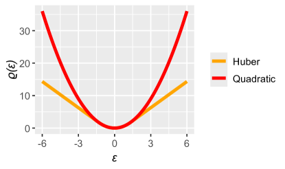
Figure 3: $\varrho$ as a function of $\varepsilon$ when $\varrho$ is the quadratic function and the $\varrho$ function associated to the Huber M-estimator with $k=1.345$.

If we interpret this M-estimator as the maximum likelihood estimator of an heavy-tailed model, we have that

$$f(\varepsilon)=\frac{g(\varepsilon)}{m}=\left\{\begin{array}[]{lcc}\exp(-\varepsilon^{2}/2)/m&\text{ if }&|\varepsilon|\leq k,\cr\exp(-k|\varepsilon|-k^{2}/2)/m&\text{ if }&|\varepsilon|>k,\cr\end{array}\right.$$

where $m=2\mathrm{e}^{-k^{2}/2}/k+\sqrt{2\pi}(2\Phi(k)-1)$.

A.2 Tukey’s biweight M-estimator

For Tukey’s biweight M-estimator, we have that

$$\varrho(\varepsilon)=-\log g(\varepsilon)=\left\{\begin{array}[]{lcc}1-(1-(\varepsilon/k)^{2})^{3}&\text{ if }&|\varepsilon|\leq k,\cr 1&\text{ if }&|\varepsilon|>k,\end{array}\right.$$

$$\psi(\varepsilon)=k^{2}\varrho^{\prime}(\varepsilon)/6=\varepsilon\left(1-(\varepsilon/k)^{2}\right)^{2}\mathds{1}(|\varepsilon|\leq k),$$

and

$$W(\varepsilon)=\left(1-(\varepsilon/k)^{2}\right)^{2}\mathds{1}(|\varepsilon|\leq k).$$

In Figure 4, we present the $\varrho$ function associated to Tukey’s biweight M-estimator. We do not present the quadratic function because the $\varrho$ function associated to Tukey’s biweight M-estimator operates on a different scale.

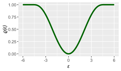
Figure 4: $\varrho$ as a function of $\varepsilon$ when $\varrho$ is the function associated to Tukey’s biweight M-estimator with $k=4.685$.

As mentioned in Section 2.1, the M-estimator can be interpreted as the maximum likelihood estimator of an heavy-tailed model, but in this case the model is improper and only the function $g$ can be identified:

$$g(\varepsilon)=\left\{\begin{array}[]{lcc}\exp\left(-1+(1-(\varepsilon/k)^{2})^{3}\right)&\text{ if }&|\varepsilon|\leq k,\cr\exp(-1)&\text{ if }&|\varepsilon|>k.\end{array}\right.$$

A.3 Student’s $t$ model

For Student’s $t$ model, we have that

$$f(\varepsilon)=\frac{\Gamma\left(\frac{\nu+1}{2}\right)}{\sqrt{\pi\nu}\,\Gamma\left(\frac{\nu}{2}\right)}\left(1+\frac{\varepsilon^{2}}{\nu}\right)^{-\frac{\nu+1}{2}}=\frac{1}{m}\left(1+\frac{\varepsilon^{2}}{\nu}\right)^{-\frac{\nu+1}{2}},\quad\varepsilon\in\operatorname{\mathbb{R}},$$

where $\Gamma$ is the gamma function, $\nu>0$ represents the degrees of freedom.

We can view maximum likelihood estimation of the model as M-estimation of the normal model. From this perspective, we have that

$$\varrho(\varepsilon)=-2\log g(\varepsilon)=(\nu+1)\log\left(1+\varepsilon^{2}/\nu\right),$$

$$\psi(\varepsilon)=\frac{\nu}{2(\nu+1)}\,\varrho^{\prime}(\varepsilon)=\frac{\varepsilon}{1+\varepsilon^{2}/\nu},$$

and

$$W(\varepsilon)=\frac{1}{1+\varepsilon^{2}/\nu}.$$

In Figure 5, we present a comparison between the quadratic function and the $\varrho$ function associated to Student’s $t$ model.

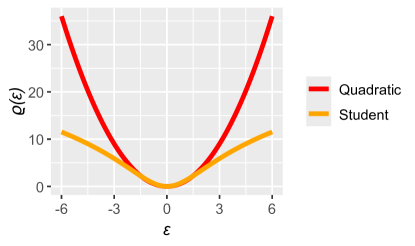
Figure 5: $\varrho$ as a function of $\varepsilon$ when $\varrho$ is the quadratic function and the $\varrho$ function associated to Student’s $t$ model with $\nu=4$.

A.4 LPTN model

For the LPTN model, we have that

$$f(\varepsilon)=\left\{\begin{array}[]{lcc}\varphi(\varepsilon)&\text{ if }&|\varepsilon|\leq\tau,\cr\varphi(\tau)\,\frac{\tau}{|\varepsilon|}\left(\frac{\log\tau}{\log|\varepsilon|}\right)^{\lambda}&\text{ if }&|\varepsilon|>\tau.\end{array}\right.$$

We can view maximum likelihood estimation of the model as M-estimation of the normal model. From this perspective, we have that

$$\varrho(\varepsilon) =-2(\log g(\varepsilon)-\log m+(1/2)\log(2\pi))$$

$$=-2(\log f(\varepsilon)+(1/2)\log(2\pi))$$

$$=\left\{\begin{array}[]{lcc}\varepsilon^{2}&\text{ if }&|\varepsilon|\leq\tau,\cr\tau^{2}-2\log(\tau)+2\log|\varepsilon|-2\lambda\log(\log\tau)+2\lambda\log(\log|\varepsilon|)&\text{ if }&|\varepsilon|>\tau,\end{array}\right.$$

$$\psi(\varepsilon)=\varrho^{\prime}(\varepsilon)/2=\left\{\begin{array}[]{lcc}\varepsilon&\text{ if }&|\varepsilon|\leq\tau,\cr\frac{1}{\varepsilon}+\frac{\lambda}{\varepsilon\log|\varepsilon|}&\text{ if }&|\varepsilon|>\tau,\end{array}\right.$$

and

$$W(\varepsilon)=\left\{\begin{array}[]{lcc}1&\text{ if }&|\varepsilon|\leq\tau,\cr\frac{1}{\varepsilon^{2}}+\frac{\lambda}{\varepsilon^{2}\log|\varepsilon|}&\text{ if }&|\varepsilon|>\tau.\end{array}\right.$$

In Figure 6, we present a comparison between the quadratic function and the $\varrho$ function associated to the LPTN model.

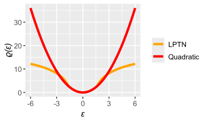
Figure 6: $\varrho$ as a function of $\varepsilon$ when $\varrho$ is the quadratic function and the $\varrho$ function associated to the LPTN model with $\rho=0.9$.

References

- Beaton and Tukey (1974) Beaton, A. E. and Tukey, J. W. (1974) The fitting of power series, meaning polynomials, illustrated on band-spectroscopic data. Technometrics, 16, 147–185.
- Bissiri et al. (2016) Bissiri, P. G., Holmes, C. C. and Walker, S. G. (2016) A general framework for updating belief distributions. J. R. Stat. Soc. Ser. B. Stat. Methodol., 78, 1103–1130.
- Desgagné (2015) Desgagné, A. (2015) Robustness to outliers in location–scale parameter model using log-regularly varying distributions. Ann. Statist., 43, 1568–1595.
- Frees (2010) Frees, E. W. (2010) Regression modeling with actuarial and financial applications. Cambridge University Press.
- Gagnon (2023) Gagnon, P. (2023) Robustness against conflicting prior information in regression. Bayesian Anal., 18, 841 – 864.
- Gagnon et al. (2020) Gagnon, P., Desgagné, A. and Bédard, M. (2020) A new Bayesian approach to robustness against outliers in linear regression. Bayesian Anal., 15, 389–414.
- Gagnon and Hayashi (2023) Gagnon, P. and Hayashi, Y. (2023) Theoretical properties of Bayesian Student- linear regression. Statist. Probab. Lett., 193 (February), 1–8.
- Gagnon and Wang (2024) Gagnon, P. and Wang, Y. (2024) Robust heavy-tailed versions of generalized linear models with applications in actuarial science. Comput. Statist. Data Anal., 194 (June), 1–16.
- Hamura et al. (2022) Hamura, Y., Irie, K. and Sugasawa, S. (2022) Log-regularly varying scale mixture of normals for robust regression. Comput. Statist. Data Anal., 173, 107517.
- Hamura et al. (2024) — (2024) Posterior robustness with milder conditions: Contamination models revisited. Statist. Probab. Lett., 210 (July), 1–5.
- Huber (1964) Huber, P. J. (1964) Robust estimation of a location parameter. The Annals of Mathematical Statistics, 35, 73–101.
- Huber (1973) — (1973) Robust regression: asymptotics, conjectures and Monte Carlo. Ann. Statist., 799–821.
- Maronna et al. (2019) Maronna, R. A., Martin, R. D., Yohai, V. J. and Salibián-Barrera, M. (2019) Robust statistics: Theory and methods (with R). John Wiley & Sons.
- O’Hagan and Pericchi (2012) O’Hagan, A. and Pericchi, L. (2012) Bayesian heavy-tailed models and conflict resolution: A review. Braz. J. Probab. Stat., 26, 372–401.
- Raftery et al. (1997) Raftery, A. E., Madigan, D. and Hoeting, J. A. (1997) Bayesian model averaging for linear regression models. J. Amer. Statist. Assoc., 92, 179–191.
- Taylor and Ashe (1983) Taylor, G. C. and Ashe, F. R. (1983) Second moments of estimates of outstanding claims. J. Econometrics, 23, 37–61.
- Verrall (1991) Verrall, R. (1991) On the estimation of reserves from loglinear models. Insurance Math. Econom., 10, 75–80.
- West (1984) West, M. (1984) Outlier models and prior distributions in Bayesian linear regression. J. R. Stat. Soc. Ser. B. Stat. Methodol., 46, 431–439.