Observation of the symmetry-protected signature of 3-body interactions
Abstract
Identifying and characterizing multi-body interactions in quantum processes remains a significant challenge. This is partly because 2-body interactions can produce an arbitrary time evolution, a fundamental fact often called the universality of 2-local gates in the context of quantum computing. However, when an unknown Hamiltonian respects a U(1) symmetry such as charge or particle number conservation, N-body interactions exhibit a distinct symmetry-protected signature known as the N-body phase, which fewer-body interactions cannot mimic. We develop and demonstrate an efficient technique for the detection of 3-body interactions despite the presence of unknown 2-body interactions. This technique, which takes advantage of GHZ states for phase estimation, requires probing the unitary evolution and measuring its determinant in a small subspace that scales linearly with the system size, making it an efficient approach.
Recent developments in quantum information science have revealed various new possibilities for generating and controlling multi-body interactions [1, 2, 3, 4, 5]. However, while such interactions can be a powerful resource in quantum computing, characterizing and identifying them also pose new challenges for standard approaches in this field. Therefore, developing new methods for detecting and learning such interactions is a timely and important goal for the field of quantum metrology and Hamiltonian learning [6, 7, 8, 9]. Multi-body interactions appear in natural physical processes and may exist fundamentally, as seen in quantum chromodynamics, or emerge within effective theories when certain degrees of freedom or subspaces are integrated out [10]. Given the successful use of quantum metrology techniques for enhancing sensor signal-to-noise such as the detection of gravitational waves in the LIGO/VIRGO experiments [11, 12], it is natural to consider the use of such techniques for detecting other elusive physical phenomena such as 3-body interactions.
A no-go theorem– Do dynamics under 3-body interactions have any distinct signatures that cannot be reproduced by 2-body interactions, making them directly detectable? As an example, consider a system with qubits interacting under a general Hamiltonian
| (1) |
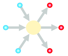
where can be decomposed as a sum of 2-local interactions, i.e., those that act non-trivially only on, at most, a pair of qubits, and denote Pauli operator on qubit . As a concrete example, one may assume contains a time-dependent XY interaction between nearest-neighbor qubits on a chain, as well as time-dependent single-qubit and fields. The Hamiltonian may describe, e.g., a spin chain or the interaction between the internal degrees of freedom of particles that interact through a scattering process (See Fig. 1).
Suppose we can prepare the system in arbitrary initial states which then evolve under the Hamiltonian from time to . By performing such experiments can we
obtain any information about the hypothetical 3-body term ? It turns out that the answer is negative.
Theorem:
Consider a unitary process described by an unknown Hamiltonian in the form of Eq.(1) for a fixed total time . Suppose one can prepare arbitrary initial states and perform arbitrary measurements on the final state, and repeat this arbitrarily many times. Unless one has further information about the term corresponding to the 2-body interactions in this Hamiltonian, it is impossible to detect the presence of 3-body interactions , or to obtain any information about their strengths .
This no-go theorem is an immediate corollary of the universality of 2-qubit gates, which is one of the cornerstones of quantum computing [13, 14]: By choosing different input states and output measurements, the only information that can be obtained about the Hamiltonian is limited to what can be inferred from the unitary operator , where denotes the time-ordered integral and we take . However, 2-body interactions in the Hamiltonian can synthesize any arbitrary unitary transformation. Therefore, adding three-body interactions does not extend the set of realizable unitaries, and thus their presence cannot be detected.
On the other hand, perhaps surprisingly, it has been recently shown that in the presence of symmetries, this no-go theorem can be violated [3]. That is, 3-body interactions have certain signatures that are protected by the symmetry of the time evolution and cannot be reproduced by 2-body interactions. Based on this observation, Ref.[3] proposes a method for detecting the locality of interactions. However, as explained below, this method requires probing the unknown unitary in the entire Hilbert space, rendering it inefficient for large systems.
In this article, we introduce a new symmetry-protected signature of 3-body interactions, denoted by the phase , and develop a method for efficient measurement of this quantity. Furthermore, we perform an experiment that measures this quantity on trapped atomic ion qubits, directly detecting the presence of 3-body interactions. A key component of our scheme, which enables efficient detection of 3-body interactions is the use of Greenberger–Horne–Zeilinger (GHZ) states [15]. Hence, our work reveals a novel application of GHZ states in the context of quantum sensing and Hamiltonian learning.
Main results
An observable phase protected by symmetry– Consider qubits evolving under Hamiltonian from time to . Assume the Hamiltonian respects the U(1) symmetry corresponding to rotations around the -axis, or equivalently, it commutes with . The unitary time evolution generated under this Hamiltonian can then be decomposed as
| (2) |
where is the component of the unitary in the subspace with “excitations”, or the eigen-subspace of with eigenvalue (also, known as the subspace with the Hamming weight ). The U(1) symmetry implies that the number of excitations is conserved under unitary , which explains the above block-diagonal form. For any such unitary, we define the phase
| (3) |
where
is the phase of the determinant of unitary . Note that since sectors are one-dimensional, and .
As we prove in Methods, the phase has the following properties: First, if the U(1)-invariant Hamiltonian only contains 2-qubit interactions, then is an integer multiple of . Therefore, indicates the presence of interactions that couple more than 2 qubits together. In particular, for Hamiltonian in Eq.(1), assuming the two-body interactions in Hamiltonian are U(1)-invariant, we show that
| (4) |
where we have defined the phase . By measuring the phase and assuming the coefficients are time-independent, we can measure the net 3-body term , up to an integer multiple of . Hence, we can uniquely determine either by measuring for a sufficiently short time , or, alternatively, by measuring the phase for a few different values of time . Also, if the interactions are translationally or permutationally invariant, this allows us to determine .
Beyond this example, for a general U(1)-invariant Hamiltonian in the Supplementay Material we establish the following remarkable identity:
| (5) |
Here, the summation is over odd integers and for , the operator , where the summation is over satisfying 111For instance, for and qubits operator and , respectively.. It follows that by adding the -body interaction acting on distinct qubits to the Hamiltonian , the phase remains unchanged for even , whereas for odd it changes linearly as
This, in particular, implies Eq.(4). It is also worth noting that the phase is additive in time. That is, by repeating the unitary sequentially times, which realizes the unitary , the corresponding phase transforms as , which can be useful for amplifying this phase if 3-body interactions are weak.
It is interesting to compare this approach with the original proposed scheme [3] based on the notion of -body phases
| (6) |
where integer is the eigenvalue of
in the sector with excitations. Note that while each -body phase depends on all , and therefore its measurement requires probing the unitary in an exponentially large Hilbert space, to determine , one only needs to probe the system in the -dimensional subspace corresponding to the sectors with , and excitations. However, this extra exponential cost of measuring -body phases comes with additional information about the locality of interactions: is only sensitive to -body interactions, i.e., unless , by
adding the -body interaction to the Hamiltonian, the -body phase remains unchanged.
It is also worth noting that in the special case of Hamiltonians in the form of Eq.(1) that only contain up to 3-body interactions,
comparing Eq.(5) and Eq.(6), we find .
The measurement scheme– Next, we introduce a method for measuring the phase . Each phase is not observable individually, because it transforms non-trivially under the global phase transformation . To overcome this and find an efficient way of measuring , we rewrite Eq.(3) as
| (7) |
Now each of the three phases , , and remains invariant under the above global phase transformation and can be experimentally measured as we demonstrate below.
First, is the relative phase between the fully occupied state and the vacuum state . Thanks to the ability to prepare the GHZ state
| (8) |
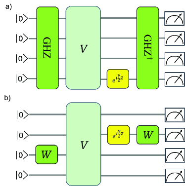
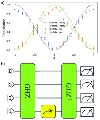
which is the equal superposition of these two states, this phase is directly observable via the standard phase sensing methods. Namely, by running the circuit (a) of Fig. 2, we measure the probability
| (9) |
for a few different values of , which uniquely determines the phase .
Next, consider the phase , which can be interpreted as the total phases obtained by single-excitation states relative to the vacuum state . Of course, standard process tomography allows the determination of , up to a global phase. However, in this way, we will not be able to detect the desired relative phase because sensing that phase requires the interference between the 0 and 1 excitation states. To achieve this, we use the circuit (b) in Fig. 2 to measure the probability
| (10) |
where and denotes the Hadamard gate on qubit . Here, are the absolute value (phase) of the matrix element
| (11) |
for , where is the state with a single excitation at qubit . Hence, by repeating this measurement for a few different values of , we can determine matrix elements . The determinant of this matrix determines the phase .
Finally, the phase , which can be interpreted as
the total phase obtained by the single-hole states relative to the fully occupied state , can be measured in a similar fashion using the circuit in Fig. 2b, except in this case all qubits should be initialized in state . Combining these three phases using Eq.(7), we find the value of , via different measurement settings.
The experiment– We perform the experiment on 5 qubits within a 7-ion programmable trapped ion quantum computer, with all-to-all connectivity, individual addressing, and efficient state readout of all qubits [16, 17, 18] (see Methods for more details). In particular, we use hyperfine qubits of 171Yb+ ions, with single-qubit gate fidelity of 99.6(2)% and two-qubit gate fidelity ranges from 99.3(1)% to 98.7(2)% for the qubit pairs used in this work (the fidelities are not corrected for state preparation and measurement [SPAM] errors estimated to be about 0.3%).
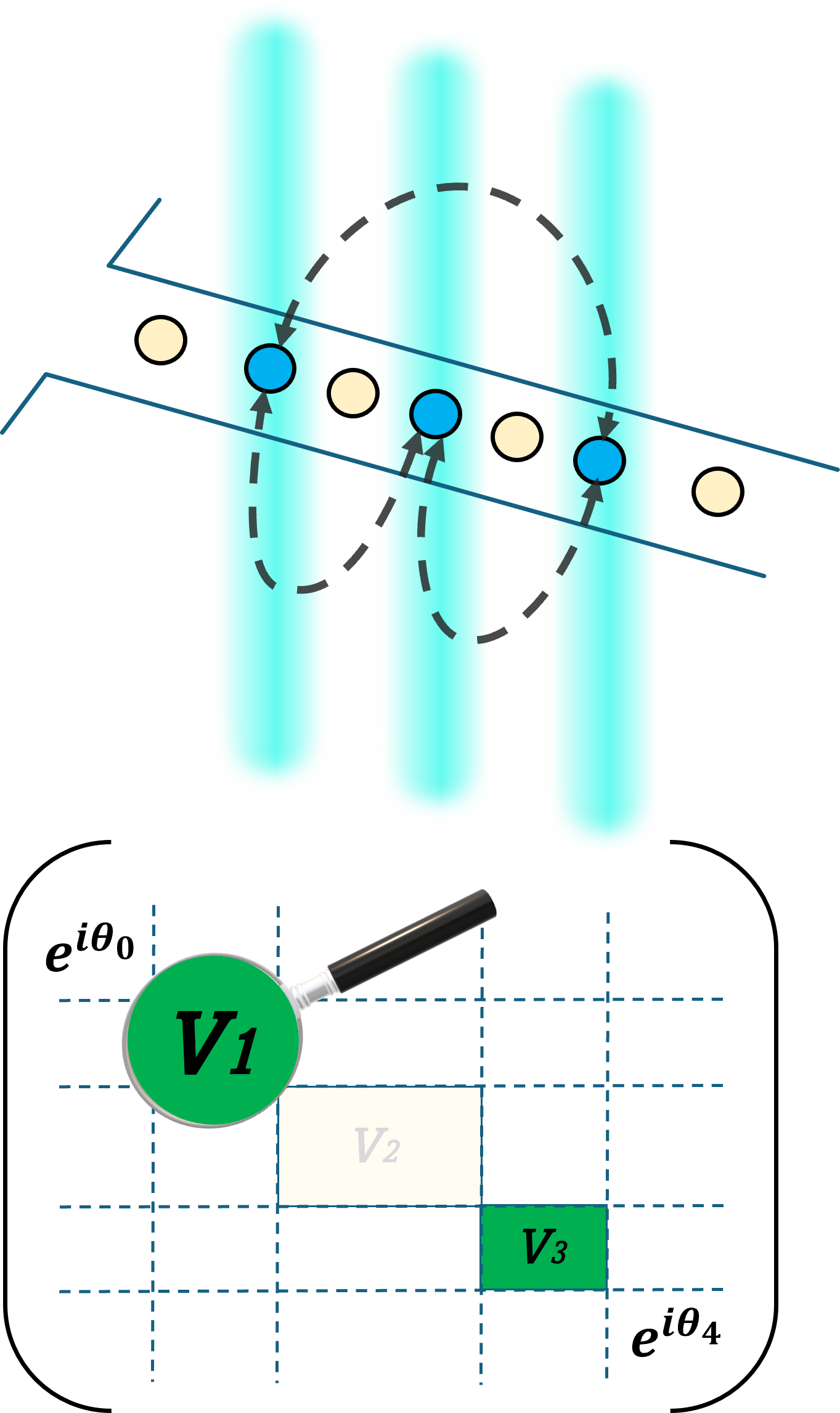
The ions are arranged in a linear chain, equidistantly spaced, and individually addressed with tightly focused beams passing through a multi-channel AOM, as depicted in the schematic of Fig. 3. The geometry of the individual addressing beams is perpendicular to the plane of the ion chain, enabling the addressing of transverse modes. With such capability, the system can implement universal gates for any qubit or pair of qubits. The native two-qubit gates are Mølmer-Sørensen or Ising operations between arbitrary pairs of qubits [19].
We employ automated calibration of single- or two-qubit gates and execute the large number of circuits required in the experiment with a periodic evaluation of the system’s performance. Namely, we utilize a software-hardware API [20] alongside an automated calibration procedure within the hardware coding environment. This API optimizes and transpiles gate-level circuits into pulse sequences, then submits these sequences to an integrated hardware control system - ARTIQ (Advanced Real-Time Infrastructure for Quantum Physics) [21]. ARTIQ manages the coordination of the hardware system to execute the pulse sequences and performs auto-calibrations as needed. By adhering to a software-hardware co-design principle, we enhance circuit execution efficiency and resilience to hardware interruptions, facilitating the handling of a large number of circuits with high performance.
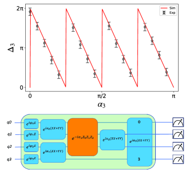
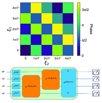
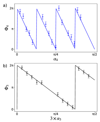
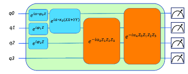
Measuring – To demonstrate this method we utilize a setup with four qubits on a trapped-ion quantum simulator (See Fig. 4). In addition to one- and two-qubit U(1)-invariant unitaries, the unknown unitary also contains the three-qubit unitary for . The two-qubit gates exchange excitations between qubits, which means the realized U(1)-invariant unitary is not diagonal in the computational basis. The phase for this circuit can be calculated from Eq.(1) to be (Note that any circuit can be interpreted as a time-dependent Hamiltonian evolution).
Then, to experimentally measure , we measure the three phases in Eq.(7)
using the circuits in Fig. 2. The plot in Fig. 4 compares the outcome of the experiment with the theoretical prediction in Eq.(4). This plot clearly shows a
distinctive feature of : it oscillates eight times faster than . Remarkably, for measuring the phase we do not need to probe the 6D subspace with excitations. We also check that the phase does not change by varying 1-qubit and 2-qubit U(1)-invariant gates (see Methods).
Additivity of – Another crucial feature of the phase is additivity: according to Eq.(4) all 3-body interactions have equal contributions in the phase . To experimentally verify this we consider the unitary in the following form changed
| (12) |
on a system with qubits, where , and are random 2-local U(1)-invariant unitaries, namely , and for random values of . As it is shown in Fig. 5, by varying the 3-body interaction strength and , we experimentally verify the additivity of the phase . Specifically, we demonstrate that , which follows from Eq.(4).
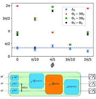
Measuring -body phases– In the last experimental setup, we measure the -body phases in Eq.(6), which unlike allows us to distinguish -body interactions, with different . However, this requires performing full tomography by probing all sectors of unitary .
In this experiment, we consider a system with qubits evolving under the unitary
| (13) |
where and are random one- and two-qubit U(1)-invariant unitaries. To simplify the experiment and presentation, rather than varying and independently, we choose a particular ratio, namely . This can be interpreted as the unitary corresponding to the Hamiltonian plus one- and two-qubit U(1)-invariant terms. Fig. 6 presents the corresponding 3-body and 4-body phases, and . As expected from Eq.(6), both and oscillate times faster than and , respectively.
To perform the process tomography on , we use a technique that takes advantage of the U(1) symmetry of this unitary.
On a system with qubits, this symmetry implies that, instead of real parameters, to specify the unitary we need to determine [22] (For the present experiment this means real numbers instead of ). Therefore, to take advantage of the symmetry constraints, rather than the standard
tomography protocols which ignore this structure, we utilize a different technique. Namely, we use variants of the circuit (b) in Fig. 2, with more Hadamard gates at the input and output, which allows the creation of more excitations.
Discussion
We introduced a new method for observing the symmetry-protected signature of 3-body interactions and performed the first-ever experiment demonstrating its measurement, enabling the direct detection of 3-body interactions. Our experiment was conducted on a trapped ion QC with an average 2-qubit gate error of 1. The possibility of such direct detection of 3-body interactions was recently revealed in [3]. While the original method proposed in [3] requires full process tomography, the new scheme introduced in this paper only probes a subspace that scales linearly with the number of qubits. To achieve this, we take advantage of GHZ states, which allow us to directly measure the relative phase between the vacuum and fully occupied states. Without GHZ states, the presence of 3-body interactions can still be detected, although the efficiency will generally be lower. For instance, in Methods, we introduce a different scheme that does not use GHZ states; however, it requires probing the system in the subspace with 1, 2, and 3 excitations, whose total dimension scales as . This alternative scheme can be useful when preparing GHZ states is challenging, e.g., when the excitations are massive.
Methods
I Path-independent observable phases protected by symmetry
The phase introduced in Eq. (3) is an example of a general formalism introduced in Ref. [3] for constructing path-independent phases under symmetric Hamiltonians. In the following, first, we review this formalism and then study the properties of phase . Finally, in Sec. I.4, we introduce another family of such phases, which provides an alternative approach for detecting 3-body interactions.
I.1 Review: The formalism of the symmetry-protected path-independent phases
Consider a system with qubits with the total Hilbert space . Let be the projector to the eigen-subspace of with eigenvalue , i.e., the subspace with excitations. Suppose this system evolves under U(1)-invariant Hamiltonian , which realizes the unitary . Then, U(1) symmetry implies that and decompose as and , where and are are components of and in the subspace with excitations, respectively. Furthermore,
| (14a) | ||||
| (14b) | ||||
Next, recall that for any pair of operators and , , which implies
| (15) |
Defining , i.e., the phase of , we conclude that for any set of integers ,
| (16) |
where . Note that is defined only mod . Therefore, the phase is well-defined only when coefficients are integers. The above argument, in particular, means that if Hamiltonians and generate the same unitary , then
| (17) |
If operator is traceless then remains invariant under a global phase transformation for any . This can be seen, e.g., using the fact that if Hamiltonian realizes , then Hamiltonian realizes . For traceless operator , remains invariant under this transformation. Then, the second equality in Eq.(16) implies that the phase remains invariant.
In summary, for any traceless operator with integer eigenvalues , the phase defined in Eq.(16) is an observable quantity. As we see next, by measuring this phase we can obtain information about the locality of the Hamiltonian .
As an example, recall the definition of operators in [3]: Operator is defined to be the identity operator on qubits, and for
| (18) |
where the summation is over that satisfy . Operators decomposes as
| (19) |
where eigenvalues
| (20) |
are all integers [3]. Ref.[3] defines the -body phase associated to the time evolution generated by the U(1)-invariant Hamiltonian , as
| (21) |
where . As explained before, by adding the -body interaction acting on distinct qubits to the Hamiltonian , remains unchanged for all , except . Therefore, by measuring we can detect -body interactions. See also [5] for the extension of this formalism to the case of SU(2) symmetry.
I.2 Localization in frequency and spatial domains
The above property of operators and the corresponding phases means that they provide sharp information about the locality of interactions. However, because for each integer the corresponding integers are typically non-zero, to measure -body phase , we need to probe the entire Hilbert space, i.e., sectors with arbitrary excitation numbers .
The operators and projectors are two different orthogonal bases, with respect to the Hilbert-Schmidt inner product, for the same operator space. That is, and
and
for all . Hence, Eq.(19) describes a change of basis from one orthogonal basis to another. Furthermore, while the basis defines a sharp notion of locality, the basis defines a sharp notion of the number of excitations (charge, or Hamming weight) in the system. The fact that integers are typically non-zero, means that each element of the basis has support on many elements of the basis . In this sense, the transformation defined by Eq.(19) is analogous to the Fourier transform, and the relation between and bases is analogous to the Fourier uncertainty relation.
As we explain next, from this point of view the phase , and the phases defined in Sec.I.4, correspond to operators that are partially localized in both spatial and frequency (charge) domains (See Fig. 7).
I.3 as a path-independent phase
Suppose in Eq.(16), we choose to be the operator
| (22) |
which has integer eigenvalues and is traceless. Then, applying Eq.(16) we find that
| (23) | ||||
To understand properties of the phase , in Appendix A we find the decomposition of operator in terms of operators. Namely, we show that
| (24) |
where the summation is over odd integers in the interval (See the middle part of Fig. 7 for a schematic representation of this equation). Putting this into Eq.(23) immediately implies Eq.(5). Furthermore, in the special case of Hamiltonians that can be decomposed as a sum of 3-body interactions, such as Hamiltonian in Eq.(1), we have for . Moreover, for distinct ,
This implies that for the time evolution under Hamiltonian in Eq.(1), we have
which proves Eq.(4). In this case
| (25) |
I.4 An alternative approach for detecting 3-body interactions
As we saw before, to measure the phase one needs to probe the subspaces with excitations. We saw that this can be achieved efficiently, provided that one can prepare GHZ states that contain superposition of states with and excitations. However, for some applications, preparing such a superposition might be unfeasible (e.g., when the excitations are massive).
For such applications, here we introduce another family of path-independent phases, which can be measured by probing the system in the sectors with excitations. Indeed, we introduce a more general formalism that allows us to detect -body interactions by probing the sectors with excitations.
For , define the phase
| (26) | ||||
where operator
| (27) |
This definition, in particular, means that operators are linearly independent, and form a basis for the operator space
| (28) |
Note that only depends on . For instance, for , we find
For the special case of qubits, we have
| (29) |
which implies .
The crucial property of operators , which is proven in the Supplementary Material, is the following: For all we have
| (30a) | ||||
| (30b) | ||||
The bottom part of Fig. 7 presents a schematic representation of Eq.(30) and Eq.(27). In particular, except , which corresponds to , the rest of operators are traceless, which means are experimentally observable. Note that according to Eq.(26), to measure , we only need to probe sectors with excitations.
Furthermore, applying this equation, in Appendix B, we show that
Lemma 1.
Suppose operator can be written as a sum of -local terms. Then,
| (31) |
and for .
This lemma implies that for U(1)-invariant Hamiltonian in the form of Eq.(1),
| (32) |
More generally, consider the Hamiltonian
| (33) |
where is an unknown U(1)-invariant Hamiltonians that does not contain -body interactions, i.e., can be decomposed as the sum of -local U(1)-invariant terms. For this Hamiltonian, we obtain
| (34) |
Further details and error analysis for the experiment
Trapped Ion Quantum Computer: We decompose the transverse modes of seven 171Yb+ ions and estimate the effect of noise and drifts on the gates [23]. This analysis is followed by constructing segmented optical pulses tailored for the entangling gates to ensure their robustness. Gate duration and pulse shaping are adjusted for individual ion pairs to minimize coupling to motion at the end of the gate pulse sequence.
The two-qubit gates fidelity measurement technique is outlined in [17]. A single-qubit gate is a composite SK1 pulse [24]. For SPAM measurement, we prepare qubits in the (dark) and (bright) states, then perform a Poisson fit to the histograms corresponding to these two states. The resulting SPAM is 0.27(4)%.
Circuit Design and Optimization: For all circuits, commuting single-qubit rotations and two-qubit XX(/4) gates are merged to minimize the circuit size. However, while the unitary operator is still subject to optimization, its content is not merged with the external circuit elements and is treated as a ‘black box’. The 3-body and 4-body unitaries and are realized using standard methods for implementing Pauli Hamiltonians, via a sequence of CNOTs [25].
Post-Processing and Statistical Error: Data presented in the main text are the result of several post-processing steps. First, we extract the population from the raw histograms for different values of . Then we perform fitting to extract observable phases. The next step is a construction of the total phases corresponding to 3- or 4-body interaction following Eq.(3) or Eq.(6), respectively.
Fig. 8 demonstrates the outcomes of the phase estimation experiment for measuring , with 4-qubit GHZ state. Specifically, we measure the population at for two distinct interaction strengths of the 3-body interaction, and . For each interaction strength, we vary (see Eq.(9)), then we perform fitting with a sinusoidal function to obtain the contrasts and ensure the correct measurement of the phase offset. According to Eq.(9), the measured phase offset determines the phase (A similar technique is used to determine the phase via Eq.(10)). In this particular example, we measure referenced in Eq.(9). We use a similar procedure followed by Eq.(10) to measure the rest of the observable phases.
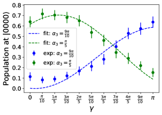
We use a statistical bootstrapping method [26] to estimate uncertainties by 1000 expectation values with each value evaluated based on a 150-shot histogram randomly resampled from the original 300-shot readout. The error bars indicate 2 from the bootstrap distribution.
Noise Model: We examine hardware error sources by directly measuring errors and simulating hardware output using the Qiskit platform [27]. We describe a two-qubit gate error in the - and -bases. For all ion pairs used in this work, the errors measured in the -basis are in the range from 0.28(5) to 0.85(4), whereas errors in the -basis are in the range from 0.01(1) to 0.04(1). The dominant noise in this model is incoherent (Pauli) error.
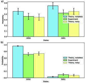
We compare output histograms to noiseless theoretical histograms, all corresponding to 300 shots. As an illustrative example, we select an experiment employing GHZ state on 4 qubits, which is often considered as the most sensitive state to noise. In Fig. 9, parts (a) and (b) correspond to two different experiments, where in (a) and , and in (b) and . To simplify the presentation, we consider probabilities only for states and , which are the only states with non-zero probability in the absence of noise (In Fig. 9 this is illustrated as ‘Theory, noiseless’).
We introduce independent single-qubit Pauli errors, according to the above noise model. The results are depicted in Fig. 9 as ‘Theory, noisy’. We apply the same error model across all qubits, assuming errors within experimentally measured ranges. With the considered noise model, one can see a good match between noisy theoretical prediction (Fig. 9, ‘Theory, noisy’) and experimental results (Fig. 9, ‘Experiment’). We compute the 1-norm of the probability vector space difference between the experiment and noisy simulation to demonstrate the agreement for the rest of the binary state subspace. The measured values do not exceed 0.05.
GHZ parity benchmark: We conduct a GHZ interference experiment to evaluate the performance of our system. When utilizing GHZ states, errors in individual qubits have a cascading effect, impacting the overall performance. Hence, such experiments provide a powerful method for benchmarking the system. Fig. 10 (b) presents a schematic of the circuit employed for these measurements, and Fig. 10 (a) displays the corresponding GHZ parity fringe observed across four qubits. We perform regular system calibrations to achieve this contrast level throughout the experiment.
Insensitivity of with respect to 1- and 2- body Interactions: In Fig. 11 we present the outcome of a 3-qubit experiment to verify that is indeed independent of one- and two-body interactions. The horizontal axis determines the phase of a single-qubit gate and two-qubit . We check that while the three phases , and all vary non-trivially with , as expected from our theoretical results, the phase does not depend on .
Circuits for and measurement:In Fig. 6 we presented the results of measuring the phases and for the 4-qubit unitary realized by the circuit in Fig. 12. As expected from Eq.(6), we observe that varying single- and two-qubit gates do not affect the measured or phases.
Acknowledgements
This work is supported by the DOE Quantum Systems Accelerator (DE-FOA-0002253), the NSF STAQ Program (PHY-1818914), the NSF QLCI grant OMA-2120757, the Army Research Office (W911NF-21-1-0005), as well as NSF grants Phy-2046195 and FET-2106448.
References
- Katz et al. [2023a] O. Katz, M. Cetina, and C. Monroe, Programmable n-body interactions with trapped ions, PRX Quantum 4, 030311 (2023a).
- Katz et al. [2023b] O. Katz, L. Feng, A. Risinger, C. Monroe, and M. Cetina, Demonstration of three-and four-body interactions between trapped-ion spins, Nature Physics 19, 1452 (2023b).
- Marvian [2022] I. Marvian, Restrictions on realizable unitary operations imposed by symmetry and locality, Nature Physics 18, 283 (2022).
- Alhambra [2022] Á. M. Alhambra, Forbidden by symmetry, Nature Physics 18, 235 (2022).
- Marvian et al. [2024] I. Marvian, H. Liu, and A. Hulse, Rotationally invariant circuits: Universality with the exchange interaction and two ancilla qubits, Physical Review Letters 132, 130201 (2024).
- V. Giovannetti, S. Lloyd, and L. Maccone [2004] V. Giovannetti, S. Lloyd, and L. Maccone, Quantum-enhanced measurements: Beating the standard quantum limit, 306, 1330 (2004).
- Giovannetti et al. [2011] V. Giovannetti, S. Lloyd, and L. Maccone, Advances in quantum metrology, Nature Photonics 5, 222 (2011).
- Degen et al. [2017] C. L. Degen, F. Reinhard, and P. Cappellaro, Quantum sensing, Reviews of modern physics 89, 035002 (2017).
- Huang et al. [2023] H.-Y. Huang, Y. Tong, D. Fang, and Y. Su, Learning many-body hamiltonians with heisenberg-limited scaling, Physical Review Letters 130, 200403 (2023).
- Hammer et al. [2013] H.-W. Hammer, A. Nogga, and A. Schwenk, Colloquium: Three-body forces: From cold atoms to nuclei, Reviews of modern physics 85, 197 (2013).
- Tse et al. [2019] M. e. Tse, H. Yu, N. Kijbunchoo, A. Fernandez-Galiana, P. Dupej, L. Barsotti, C. Blair, D. Brown, S. Dwyer, A. Effler, et al., Quantum-enhanced advanced ligo detectors in the era of gravitational-wave astronomy, Physical Review Letters 123, 231107 (2019).
- Acernese et al. [2019] F. Acernese, M. Agathos, L. Aiello, A. Allocca, A. Amato, S. Ansoldi, S. Antier, M. Arène, N. Arnaud, S. Ascenzi, et al., Increasing the astrophysical reach of the advanced virgo detector via the application of squeezed vacuum states of light, Physical review letters 123, 231108 (2019).
- DiVincenzo [1995] D. P. DiVincenzo, Two-bit gates are universal for quantum computation, Physical Review A 51, 1015 (1995).
- Lloyd [1995] S. Lloyd, Almost any quantum logic gate is universal, Physical Review Letters 75, 346 (1995).
- Greenberger et al. [1989] D. M. Greenberger, M. A. Horne, and A. Zeilinger, Going beyond bell’s theorem, in Bell’s theorem, quantum theory and conceptions of the universe (Springer, 1989) pp. 69–72.
- Nam et al. [2020] Y. Nam, J. Chen, N. Pisenti, and et al., Ground-state energy estimation of the water molecule on a trapped-ion quantum computer, npj Quantum Information 6, 10.1038/s41534-020-0259-3 (2020).
- Egan et al. [2021] L. Egan, D. Debroy, C. Noel, and et al., Fault-tolerant control of an error-corrected qubit, Nature 598, 10.1038/s41586-021-03928-y (2021).
- Cetina et al. [2022] M. Cetina, L. Egan, C. Noel, M. Goldman, D. Biswas, A. Risinger, D. Zhu, and C. Monroe, Control of transverse motion for quantum gates on individually addressed atomic qubits, PRX Quantum 3, 010334 (2022).
- Srensen and Mlmer [1999] A. Srensen and K. Mlmer, Quantum Computation with Ions in Thermal Motion, Phys. Rev. Lett. 82, 1971 (1999).
- Wang et al. [2024] Q. Wang, L. Zhukas, Q. Miao, A. S. Dalvi, P. J. Love, C. Monroe, F. T. Chong, and G. S. Ravi, Demonstration of a cafqa-bootstrapped variational quantum eigensolver on a trapped-ion quantum computer, arXiv preprint arXiv:2408.06482 (2024).
- Bourdeauducq et al. [2016] S. Bourdeauducq, R. Jördens, P. Zotov, J. Britton, D. Slichter, D. Leibrandt, D. Allcock, A. Hankin, F. Kermarrec, Y. Sionneau, R. Srinivas, T. R. Tan, and J. Bohnet, Artiq 1.0 (2016).
- Bai and Marvian [2023] G. Bai and I. Marvian, Synthesis of energy-conserving quantum circuits with xy interaction, arXiv preprint arXiv:2309.11051 (2023).
- Wu et al. [2018] Y. Wu, S.-T. Wang, and L.-M. Duan, Noise analysis for high-fidelity quantum entangling gates in an anharmonic linear paul trap, Phys. Rev. A 97, 062325 (2018).
- Brown et al. [2004] K. R. Brown, A. W. Harrow, and I. L. Chuang, Arbitrarily accurate composite pulse sequences, Phys. Rev. A 70, 052318 (2004).
- Nielsen [2001] M. Nielsen, Universal quantum computation using only projective measurement, quantum memory, and preparation of the 0 state (2001), quant-ph/0108020 .
- Efron and Tibshirani [1994] B. Efron and R. Tibshirani, An Introduction to the Bootstrap (Chapman and Hall/CRC, New York, 1994).
- Javadi-Abhari et al. [2024] A. Javadi-Abhari, M. Treinish, K. Krsulich, C. J. Wood, J. Lishman, J. Gacon, S. Martiel, P. D. Nation, L. S. Bishop, A. W. Cross, B. R. Johnson, and J. M. Gambetta, Quantum computing with Qiskit (2024), arXiv:2405.08810 [quant-ph] .
oneΔ
oneΔ
oneΔ
Supplementary Material:
Observation of the symmetry-protected signature of 3-body interactions
Appendix A Properties of phase (Proof of Eq.(5))
In this Appendix, we prove Eq.(5). To prove this equation it is useful to remember some properties of operators
| (35) |
where the eigenvalues
| (36) |
are all integers. It can be easily seen that , i.e., under applying Pauli on all qubits the -excitation sector is transformed to -hole sector. Furthermore, since is decomposed as a sum of tensor products of Pauli operators, we find . This, in particular, implies
| (37) |
Operators are linearly independent and satisfy the orthogonality relation
| (38) |
It follows that the subspace spanned by is equal to the subspace spanned by operators . This subspace has dimension . This is indeed the subspace of operators that commute with U(1)-invariant Hamiltonians.
Any operator has a decomposition as
| (39) |
with the property that
| (40) |
Applying this decomposition to operator , we find that
| (41) |
Using the facts that and , we find that
| (42) |
which implies for even .
Appendix B An alternative approach for detecting 3-body interactions (Properties of phase and operator )
We prove that for all , it holds that
| (52) |
The proof is presented at the end of this section. For , the left-hand side of this equation becomes
| (53) |
which means except the rest of are traceless.
For , the right-hand side of Eq.(52) is equal to
| (54) |
The left-hand side, on the other hand, becomes
| (55) |
where is the smallest value of for which is non-zero. Comparing the two sides, we can immediately see that
| (56a) | ||||
| (56b) | ||||
Next, using this identity we prove lemma 1.
It is also worth noting that by taking derivatives with respect to of both sides of Eq.(52), at , this equation implies
| (57) |
B.1 Proof of lemma 1
First, using Eq.(39) we find
| (58) |
Since is a linear combination of operators, Eq.(40) implies . Therefore, we find
| (59) | ||||
| (60) |
where to get the second line we have used the assumption that can be written as a sum of -local terms, and therefore it is orthogonal to operator for . Applying Eq.(56), we find that for , , and for
| (61) | ||||
| (62) | ||||
| (63) | ||||
| (64) |
This proves lemma 1.
B.2 Proof of Eq.(52)
First, using the Euler formula , we find
| (65) | ||||
| (66) | ||||
| (67) |
This implies that
| (68) |
Next, we use the fact that
| (69) |
and
| (70) |
This implies
| (71) | ||||
| (72) | ||||
| (73) | ||||
| (74) | ||||
| (75) |
In summary, we found
| (76) | ||||
| (77) | ||||
| (78) |
Comparing this with Eq.(68) ,we find
| (79) |
or, equivalently,
| (80) |