Price Competition Under A Consider-Then-Choose Model With Lexicographic Choice

Abstract

The sorting and filtering capabilities offered by modern e-commerce platforms significantly impact customers’ purchase decisions, as well as the resulting prices set by competing sellers on these platforms. Motivated by this practical reality, we study price competition under a flexible choice model: Consider-then-Choose with Lexicographic Choice (CLC). In this model, a customer first forms a consideration set of sellers based on (i) her willingness-to-pay and (ii) an arbitrary set of criteria on items’ non-price attributes; she then chooses the highest-ranked item according to a lexicographic ranking in which items with better performance on more important attributes are ranked higher. We provide a structural characterization of equilibria in the resulting game of price competition, and derive an economically interpretable condition, which we call gradient dominance, under which equilibria can be computed efficiently. For this subclass of CLC models, we prove that distributed gradient-based pricing dynamics converge to the set of equilibria. Extensive numerical experiments show robustness of our theoretical findings when gradient dominance does not hold.

1 Introduction

The rise of the e-commerce platform economy has introduced fundamental changes to the environment in which sellers price their goods and services. In particular, the supply diversity available on these platforms has impacted customer behavior in two important, related ways:

1. Customers are now faced with the burden of choice, with a plethora of seller offerings differing across a range of attributes such as price, quality, and popularity.

2. Limited in time and information, customers increasingly rely on platforms’ sorting and filtering functionalities to search for offerings (Ansari and Mela,, 2003; Granka et al.,, 2004; Joachims et al.,, 2005; Ghose and Yang,, 2009; Gao et al.,, 2022), and often resort to “fast and frugal” decision-making heuristics to make a final selection (Kohli and Jedidi,, 2007; Bansal and Maglaras,, 2009; Gallego et al.,, 2023).

The goal of this paper is to study equilibrium pricing outcomes that arise on e-commerce platforms as a result of these salient features of customer behavior. Tractably predicting market outcomes in these environments is important for platform operators, who can use the resulting insights to guide design decisions. For instance, platform operators can use predicted outcomes to design more effective search functionalities; they can use these predictions to monitor anomalies and identify potential collusion between sellers; in the case of equilibrium multiplicity, they can find ways to nudge sellers in the direction of welfare-optimal equilibria. However, the complexity of these environments emerging from product diversity, customer preference diversity, and platform design makes analyzing outcomes of price competition particularly challenging. This complexity further exacerbates the basic concern that computing equilibria is notoriously hard, even in discrete two-player games (Daskalakis et al.,, 2009). Hence, predicting market outcomes in these intricate environments requires models of price competition that achieve two conflicting objectives: (i) they must be flexible enough to capture platform-mediated customer choice behavior on these platforms, and (ii) they must be conducive to tractable equilibrium computation and analysis.

Toward attaining these objectives, we consider a model of purchase behavior that is specifically tailored to capture customers’ response to platforms’ filtering and sorting capabilities, and that generalizes lexicographic choice, a decision-making heuristic for multi-attribute choice that has been extensively studied and empirically validated in the behavioral economics and marketing literature (Alexis et al.,, 1968; Fishburn,, 1974; Parkinson and Reilly,, 1979; Kohli and Jedidi,, 2007; Jedidi and Kohli,, 2008; Kohli et al.,, 2019). In this model — which we call Consider-then-Choose with Lexicographic Choice — customer decision-making is composed of two phases. The first phase, which models the use of platforms’ filtering capabilities, involves the formation of a consideration set of options. In this phase, customers narrow down the set of feasible options by specifying (i) desirable non-price features (e.g., brand, rating range, size and specifications, etc.) and (ii) an upper bound on the price, reflecting their budget or maximum willingness-to-pay. The second phase involves the selection from this set according to the lexicographic choice heuristic. Specifically, customers have heterogeneous preference orderings over item attributes (e.g., price, quality, number of reviews), capturing which attributes they consider more important than others, and a (weak) ranking of items along each attribute. They first rank items with respect to their most preferred attribute, and choose the most desirable product according to that attribute. If they are indifferent amongst multiple products within this attribute-specific ranking, they evaluate the topmost products according to their second-most preferred attribute, choosing the top product for that attribute, and so on.

The CLC model generalizes the basic lexicographic choice heuristic by incorporating the consideration phase in customers’ decision-making process. In addition to naturally modeling platforms’ filtering functionalities, the notion that customers form a consideration set before choosing from a large range of options has also been empirically validated in the literature. Indeed, consider-then-choose models have been studied in areas spanning marketing, behavioral economics, and operations management (Jagabathula and Rusmevichientong,, 2017; Aouad et al.,, 2021; Jagabathula et al.,, 2020). The consideration phase moreover addresses a weakness of the vanilla lexicographic heuristic, illustrated by the following example. Consider for instance a setting in which there are two items defined by price and average rating, with one item priced at $99 with a 2-star average rating, and one item priced at $100 with a 5-star average rating. Under the basic lexicographic preference model, all customers who place higher importance on price over rating would choose the $99 item. In practice, however, the choice of a drastically lower-quality item with only a marginally better price may be difficult to justify, even if the customer places a higher importance on price. The consideration phase addresses this weakness by allowing customers to specify acceptable ranges of different attributes (e.g., quality), for the formation of their consideration set. Once such guardrails on the acceptability of choices is specified, it becomes much more reasonable for the customer to resort to the simple lexicographic choice heuristic to make her final purchase decision. In the example above, the lower-rated item may simply not be included in the consideration set, despite its lower price, because its quality is lower than what is acceptable to the customer.

In addition to the strong empirical foundations of its two phases, the CLC class encompasses several anecdotally reported purchase behaviors. One prominent example is the “Best-I-Can-Afford” (BICA) model, in which items are defined by two attributes, price and quality, and customers have heterogeneous budgets (or willingness-to-pay) for the item. Customers only include items within their budget in their consideration set, and subsequently choose the highest-quality item in this consideration set (breaking any ties according to price, and then arbitrarily). Such behavior is common among quality-sensitive customers, as well as delegated purchasers (such as customers who can claim the purchase as a business expense). Example 1.1 below illustrates that the CLC model encompasses a wide range of behaviors, in addition to BICA.

Example 1.1.

Consider a set of third-party sellers listing athletic T-shirts for women, with attributes $\{\texttt{brand},\texttt{average rating},\texttt{number of reviews},\texttt{price}\}$. The brand attribute takes values in the set $\{\texttt{Nike},\texttt{Adidas},\texttt{Puma}\}$; each T-shirt has an average rating in $[0,5]$; and the number of reviews is in $\mathbb{N}$. The following three customers belong to the CLC class:

• A price-sensitive customer. This customer is willing to pay at most $25 and requires an average rating of at least 3. Of all such items, the customer chooses the cheapest one. If there are many lowest-priced items, she chooses the one with the highest rating, and breaks final ties by number of reviews.

• A quality-sensitive customer. This customer is willing to pay at most $80 and requires an average rating of at least 4.5 with at least 100 reviews. Of all such items, she chooses the one with the highest average rating, breaking ties according to the number of reviews, followed by price.

• A loyal customer. This customer is willing to pay $100 and only considers Nike products. Of all such products, she purchases the highest rated one, breaking ties according to the number of reviews, followed by price.

The CLC model is a compelling candidate for our goal of studying price equilibria in these environments, given the heterogeneity of purchase behaviors it captures, and its clear correspondence to platform search functionalities. However, the wide heterogeneity of behaviors it subsumes makes the analysis of these outcomes seem a priori challenging. Given this, we seek to answer the following research questions: Is equilibrium computation tractable under CLC choice? Do there exist mechanisms by which predicted equilibria naturally arise on these platforms, where pricing is inherently decentralized and algorithmic?

1.1 Main contributions

Our first main finding is that for any CLC model, a unifying property emerges in the resulting game of price competition that has important implications for tractability of equilibrium computation. Under this property, which we call the pseudo-competitive property, the revenue of any seller, given other sellers’ prices, is invariant under changes to any strictly lower competing price, as long as this price remains strictly lower (Theorem 4.5). This property can easily be seen to hold in the most well-known model of price competition, Bertrand competition (Bertrand,, 1883), which belongs to the CLC class. In this latter model, customers always purchase the lowest-priced item; hence, the revenue of a seller is identically zero as long as another seller prices strictly below this first seller, irrespective of the actual price of the lower-priced seller. Our key insight is that the pseudo-competitive property is satisfied for any CLC choice model (or mixtures therof).

We use this fact to show that any equilibrium outcome has a sequential-move structure, despite the fact that it is a simultaneous-move game. In particular, we show that any local Nash equilibrium (a generalization of the notion of pure-strategy Nash equilibrium well-suited for algorithmic pricing (Ratliff et al.,, 2016)) corresponds to an ordering over sellers and a corresponding sequence of locally-optimal undercutting prices (Theorem 4.7). Under mild regularity conditions, this characterization provides a tractable procedure for computing all local Nash equilibria (and hence, all pure-strategy Nash equilibria) (Corollary 4.8), when the number of sellers is small. In contrast, as noted above, equilibrium computation is generally hard, even for the simple case of two-player matrix games (Daskalakis et al.,, 2009).

Although our structural result enables tractable equilibrium computation when the number of sellers is small, it fails to shed light on when an equilibrium is guaranteed to exist. Moreover, it shows that determining existence for general CLC models has an unavoidable factorial dependence on the number of sellers. We however identify a sufficient condition — gradient dominance — under which a local Nash equilibrium is guaranteed to exist, and equilibrium computation has polynomial dependence on the number of sellers (Proposition 4.9). This condition models settings in which certain sellers have a competitive advantage along a non-price attribute (e.g., quality), and holds under practical special cases of CLC choice, prominently including BICA behavior.

While these results are useful from the platform’s perspective, the question remains of how such LNE arise in practice (assuming they exist) remains, since sellers operating on platforms only observe their own revenue, and not their competitors’. We first investigate this question theoretically, under the gradient dominance assumption. We show that sellers using simple local price updates (formalized via distributed gradient ascent, see Algorithm 1) indeed converge to a local Nash equilibrium under mild additional regularity conditions (Theorem 5.1). We then investigate the robustness of this phenomenon numerically, and observe that for a wide range of CLC models in which customers choose based on price and rating, but in which gradient dominance may not hold, price dynamics frequently converge to a LNE. This observation is robust to more practical implementations of gradient-driven update schemes (e.g., asynchronous updates, zeroth order feedback), as well as to the limited inclusion of customers who make their purchase decisions according to the multinomial logit choice model.

Overall, our work demonstrates that the CLC choice model is able to capture a variety of practical purchase behaviors on e-commerce platforms, explicitly modeling customer search and selection, all the while (i) enabling the tractable analysis of equilibrium pricing outcomes and (ii) supporting natural distributed mechanisms for the emergence of equilibria. While the goal of this paper is not to advocate for this model to replace well-established random utility maximization models, we view it as a valuable addition to platforms’ modeling toolkits.

1.2 Paper organization

We survey relevant literature in Section 2. In Section 3 we formalize the CLC choice model, and characterize the structure of equilibria under this model in Section 4. We subsequently investigate convergence of gradient-based pricing algorithms numerically and in theory in Section 5. Unless specified, the proofs of all results are included in the appendix.

2 Related work

Our work relates to a wide range of customer choice models studied in the literature and their impact on competitive outcomes. We discuss the relevant literature below.

Lexicographic preference models. As noted above, lexicographic preferences have been extensively studied within the behavioral economics and marketing literature; see Fishburn, (1974) for an excellent survey of earlier work.

Lexicographic choice is a special case of boundedly rational behavior, the existence of which was first posited by Herbert Simon in his Nobel Prize winning work (Simon,, 1955, 1956). It is a noncompensatory rule, wherein individuals fail to evaluate fine-grained trade-offs when faced with multiple alternatives, due in part to negative emotions associated with high cognitive load (Luce et al.,, 1997; Drolet and Frances Luce,, 2004). In the empirical literature, Payne, (1976) found that, though utility-maximizing decision rules were more likely to be used in two-alternative situations, as the number of alternatives increased, subjects used non-rationalizable heuristics to eliminate some of the available alternatives as quickly as possible. Hogarth and Karelaia, (2005) showed that simple trade-off-avoiding strategies can be remarkably effective in yielding the same choices as linear multi-attribute models that explicitly account for trade-offs for binary-valued attributes. More recently, Jagabathula and Rusmevichientong, (2019) analyzed weekly sales transactions of consumer packaged goods for grocery and drug store chains for 47 markets across the United States, and found that random utility maximization (RUM) models did not yield acceptable predictive performance for a number of goods such as coffee, yogurt, and milk; they suggest that going beyond rational choice models is necessary to obtain acceptable predictive performance for these goods.

Of the many noncompensatory rules proposed in the literature, we focus on the lexicographic model due to its applicability to the existing sorting functionalities on e-commerce platforms. Prominent works that find empirical evidence of lexicographic choice include Slovic, (1975). In a laboratory experiment, participants were asked to choose between two gift packages of cash and coupons that they had decided were equal in value a week earlier, in addition to indicating whether they considered cash or coupons to be more important. Instead of choosing the two gift packages with equal probability — as a utility maximization model would have found — 88% of participants chose the alternative that was higher on the attribute they found more important (typically, cash). Within retail settings, studies have found that lexicographic models can perform as well as common utility maximization models in predicting customers’ purchase decisions. For instance, for women’s clothing Alexis et al., (1968) found that a lexicographic order over criteria such as type, size, color and style, comfort and fit, and price tends to be used in decision-making, with the first piece of clothing acceptable on all counts being purchased. Parkinson and Reilly, (1979) similarly found this to hold for toothpaste and deodorant; Kohli and Jedidi, (2007); Jedidi and Kohli, (2008); Kohli et al., (2019) and Yee et al., (2007) have all found evidence of lexicographic choice rules for electronics purchases (e.g., smartphones, tablets, computers, and television sets). Harris et al., (2018) also recently found strong evidence of the use of a lexicographic decision rule among smokers deciding between two types of cigarette packages. From a theoretical perspective, of note is Kohli and Jedidi, (2007), who obtain necessary and sufficient conditions under which a linear utility function represents a lexicographic decision rule.

A number of works have considered the problem of inferring lexicographic choice rules from data (Schmitt et al.,, 2006; Kohli and Jedidi,, 2007; Jedidi and Kohli,, 2008; Yaman et al.,, 2008; Liu and Truszczynski,, 2015; Bräuning et al.,, 2017; Kohli et al.,, 2019; Hüyük et al.,, 2022). From the platform’s perspective, predicting equilibrium outcomes would first require the estimation of the underlying lexicographic rule; existing methods can thus be used for this task. We highlight that our results on convergence of gradient-based methods imply that sellers can be model-agnostic when setting prices; relying on local information via the use of, e.g., A/B tests suffices to converge to a local optimum.

Despite its prominence in the computer science and marketing literature, the use of lexicographic models in the operations literature remains rather limited, with a few exceptions. Soberman and Sadoulet, (2007) study how political campaign budgets affect advertising strategies, and assume that voters’ decisions are represented by a lexicographic rule with two attributes, valence (i.e., inherent attractiveness of candidate) and party position, with valence being the more important attribute. Bansal and Maglaras, (2009) study the product design problem of a monopolist when customers purchase the cheapest product above a quality floor (note that this is a special case of CLC choice). Stamatopoulos et al., (2019) study dynamic pricing as a means of managing inventory costs when strategic consumers can time their purchases. They assume individuals exhibit lexicographic preferences over price and wait times: a customer always prefers to wait for a better price, but given the same price she prefers to purchase earlier rather than later. To the best of our knowledge, we are the first to study price competition under lexicographic choice.

Consider-then-choose models. The first stage of CLC choice uses the now widely accepted consider-then-choose heuristic in assortment optimization. As discussed for lexicographic choice, the consider-then-choose model was inspired by the finding that people often utilize simple decision-making heuristics to narrow their options (Howard and Sheth,, 1969; Gigerenzer and Selten,, 2002) and lessen the cognitive burden of making multi-alternative decisions (Tversky and Kahneman,, 1974). Numerous empirical studies have supported this notion. Hauser’s seminal work in this area demonstrated that consideration sets could significantly explain variation in customers’ choice decisions (Hauser,, 1978). Subsequent research has supported the observation that two-stage decision models that combine consideration set formation followed by choice typically yield more accurate predictions (Swait and Ben-Akiva,, 1987; Roberts and Lattin,, 1991; Lynch et al.,, 1991; Roberts and Lattin,, 1997). There also exists an extensive body of literature focused on rational agent models that justify consideration sets. In such models, screening heuristics have been shown to be rational under search costs (Hauser and Wernerfelt,, 1990) and constraints of limited time and knowledge (Roberts and Lattin,, 1991; Gigerenzer and Goldstein,, 1996). Consideration sets are of high relevance in the platform economy since their formation is enabled by the filtering functionalities offered by most platforms.

Consider-then-choose models have been used to great success in assortment optimization. On the estimation front, Jagabathula et al., (2024) show how consider-then-choose models can be estimated from sufficiently rich choice data despite the fact that consideration sets are unobservable. On the decision-making front, these have been proposed as compelling alternatives to standard RUM models for improved computational tractability, in addition to being more capable of handling customer preference heterogeneity (Aouad et al.,, 2021). Jagabathula and Rusmevichientong, (2017) make a similar observation by considering assortment optimization and pricing under a consider-then-choose model where the consideration set formation is predicated on a price ceiling in the first stage, and the selection of the item is made according to an exogenously given preference list. They show that under mild assumptions on how prices impact the distribution of product rankings, the joint assortment planning and pricing problem becomes tractable. Our findings align with these in obtaining tractability and the ability to capture preference heterogeneity in the analysis of price competition by assuming that customers’ preference lists are created lexicographically.

Sequential search models. In the past two decades, a large body of work has identified the sequential nature of customer search on platforms: given a set of ranked search results, customers largely browse products one by one, top to (potentially) bottom (Ansari and Mela,, 2003; Granka et al.,, 2004; Joachims et al.,, 2005; Ghose and Yang,, 2009). As a result, boundedly rational sequential search procedures (of which CLC choice is a special case) have attracted attention in the operations literature of late. For instance, Chen et al., (2021) consider a retailer’s joint assortment and ranking problem when customers with randomly drawn patience levels examine products sequentially, and purchase the first examined product deemed satisfactory. The probability with which a product is satisfactory is independent of all other products; if a customer has previously examined a product, she no longer considers it in her decision to purchase the currently examined item. This assumption is referred to as the no-revisit assumption, and implies that, even if the product used to be in the customer’s consideration set, if it is not currently then the customer will not use it as a point of comparison with her current consideration set. The no-revisit assumption is implicit in CLC choice, since a product that is not considered topmost along an attribute considered early on will never be considered again. It is precisely why customers do not evaluate trade-offs under our model. Gao et al., (2022) similarly make this assumption for the problem of monopolist pricing under a general Cascade Click model, and provide an excellent survey of works in empirical marketing and behavioral economics that rely on this modeling assumption. Our work differs from these papers since they consider a monopolist’s problem. We, on the other hand, are interested in analyzing equilibrium outcomes of price competition between sellers on an e-commerce platform. Moreover, these models assume that the monopolist uses a single ranking as a lever, to be viewed by all customers. CLC choice models the reality that there are many ways in which customers may sort and filter search results, and explicitly models this heterogeneity.

The theoretical economics literature has shown that sequential search procedures can arise when utility-maximizing customers explicitly incorporate search costs in decision-making (Weitzman,, 1979; Chen and He,, 2011; Athey and Ellison,, 2011; Salant,, 2011; Board and Pycia,, 2014). Hence, search costs have been used as a way to explain price disperson in competitive environments (Stigler,, 1961); see Anderson and Renault, (2018) for an excellent survey. As pointed out by Choi et al., (2018), much of the existing work confines itself to simple settings (e.g., symmetric duopoly environments, homogeneous consumers), given the complexity of incorporating endogenous search. Rather than attempting to derive lexicographic choice as an equilibrium response to sellers’ pricing strategies, our modeling approach is aligned with the operations literature, which treats customer behavior as exogenous. Such an approach is practical in fast-paced algorithmic pricing environments where it is challenging for customers to anticipate prices set by sellers firms before inspection. Moreover, in doing so we are able to incorporate a wide range of preferences.

Price competition under linear and attraction demand models. Compared to the economics literature, our work is more closely related to studies of price competition under exogenous models of customer behavior; see Vives, (1999) and Gallego et al., (2006) for excellent surveys. By and large, this literature seeks to characterize conditions for existence and uniqueness of pure-strategy Nash equilibria under the assumption that customers are utility-maximizing. Seminal works include Topkis, (1979) and Milgrom and Roberts, (1990), who respectively show existence of equilibria in supermodular games and monotone transformations thereof. Caplin and Nalebuff, (1991) derive separate sufficient conditions on customers’ utility functions for existence and uniqueness of equilibria among differentiated products.

A considerable focus in subsequent literature has been on logit-based choice models. Anderson et al., (1992) and Bernstein and Federgruen, (2004) established existence and uniqueness of equilibria under the MNL model with a single customer class under symmetric and asymmetric firms, respectively. Gallego et al., (2006) show existence and uniqueness in a Bertrand oligopoly for an attraction demand model with convex costs; they moreover show linear convergence to the unique equilibrium under a tâtonnement scheme. Gallego and Wang, (2014) and Aksoy-Pierson et al., (2013) later on characterize Nash equilibria under nested logit choice and mixed MNL demand under mild conditions, respectively.

Equilibrium convergence in repeated price competition under gradient-based methods. Our work joins a small line of papers that study convergence of simple gradient-based schemes in games of repeated price competition. Such schemes have attracted significant attention due to their simplicity and their widespread use in industry. Cooper et al., (2015) analyze price dynamics when two sellers estimate parameters of the underlying linear demand model without explicitly incorporating competition, and identify conditions under which sellers’ prices converge to (i) the Nash equilibrium, (ii) the cooperative solution which maximizes their joint revenue, or (iii) limit points that are neither of the two. For duopolistic price competition with linear demand and reference effects, Golrezaei et al., (2020) show that sellers running Online Mirror Descent with decreasing stepsizes converge to a stable Nash equilibrium, a solution concept tailored to reference prices. Most recently, Goyal et al., (2023) leveraged the tâtonnement scheme of Gallego et al., (2006) to show that under unknown MNL demand, sellers running a version of stochastic online gradient descent in the space of aggregated logit parameters converge to the unique Nash equilibrium.

For more general games, it is well-known that gradient-based methods can fail to converge (Mertikopoulos et al.,, 2018). The first positive result in this regard was that of Rosen, (1965), who showed that under a condition termed diagonal strict concavity (DSC), a Nash equilibrium exists and is unique; moreover, distributed gradient dynamics converge to the Nash outcome. More recently, Bravo et al., (2018) showed that under diagonal strict concavity, no-regret learning based on mirror descent almost surely converges to the unique Nash equilibrium. In the same vein, Mertikopoulos and Zhou, (2019) defined the notion of variationally stable equilibrium that attracts gradient-based dynamics in games that may not satisfy DSC.

We note that none of these regularity conditions are assumed hold in our model; in fact, revenue functions may even be discontinuous under CLC choice. So, while convergence to the pure-strategy Nash equilibrium is a natural desideratum when this equilibrium exists and is unique, in settings such as ours where sellers’ revenue curves are ill-behaved and exhibit potentially many strict local maxima, one need not expect convergence of gradient methods to these outcomes (analogous to gradient methods only converging to local optima in monopolist settings). Our setup thus requires us to expand our solution concept to local Nash equilibria, as opposed to pure-strategy Nash equilibria.

3 Model

We consider a game of price competition in which $N$ sellers, denoted by $\mathcal{N}\mathrel{\mathop{\mathchar 58\relax}}=\{1,\ldots,N\}$, each offering a specific item for sale, are faced with a unit mass of customers, each seeking to purchase a single item. Each item has a price set by its seller, as well as a set of $K$ non-price attributes, denoted by $\mathcal{A}\mathrel{\mathop{\mathchar 58\relax}}=\{1,\ldots,K\}$. We use $0$ to denote the price attribute and let $\bar{\mathcal{A}}\mathrel{\mathop{\mathchar 58\relax}}=\{0,1,\ldots,K\}$ be the set of all attributes. Attribute $k\in\bar{\mathcal{A}}$ is associated with a set $\mathcal{V}^{k}$ of possible values; we allow $\mathcal{V}^{k}$, for $k\in\mathcal{A}$, to be arbitrary, and assume that $\mathcal{V}^{0}=[0,\bar{v}]$ for some finite $\bar{v}>0$ for the price attribute. For $i\in\mathcal{N}$ and $k\in\bar{\mathcal{A}}$, let $v^{k}_{i}\in\mathcal{V}^{k}$ denote the value of attribute $k$ of the item sold by seller $i$ (also referred to as item $i$).

Each customer $c$ has a strict ranking $\succ_{c}$ over attributes in $\bar{\mathcal{A}}$, representing attributes’ relative importance to the customer. Moreover, for each attribute $k\in\bar{\mathcal{A}}$, the customer has a weak preference relationship $\succsim^{k}_{c}$ over elements of $\mathcal{V}^{k}$. In particular, for any $v\neq v^{\prime}$, $v\succ^{k}_{c}v^{\prime}$ denotes that customer $c$ prefers value $v$ over $v^{\prime}$ for attribute $k$, and $v\sim^{k}_{c}v^{\prime}$ denotes that $c$ is indifferent between $v$ and $v^{\prime}$. If $v=v^{\prime}$, we assume $v\sim^{k}_{c}v^{\prime}$. This preference relation is transitive, i.e., if $v$ is (weakly) preferred to $v^{\prime}$, and $v^{\prime}$ is (weakly) preferred to $v^{\prime\prime}$, then $v$ is (weakly) preferred to $v^{\prime\prime}$. The preference relationship for any non-price attribute may vary arbitrarily across customers; however, all customers prefer a lower price. Formally, for all $c$, $p<p^{\prime}\iff p\succ^{0}_{c}p^{\prime}$, and $p=p^{\prime}\iff p\sim^{0}_{c}p^{\prime}$.

The choice model we consider is partially defined by the lexicographic heuristic (Fishburn,, 1974).

Definition 3.1 (Lexicographic preferences).

Customer $c$ lexicographically prefers item $i$ to item $j$ if there exists an attribute $k$ such that:

1. $c$ is indifferent between $i$ and $j$ for all attributes considered more important than $k$:

   $$v_{i}^{k^{\prime}}\sim^{k^{\prime}}_{c}v_{j}^{k^{\prime}}\quad\forall\ k^{\prime}\text{ s.t. }k^{\prime}\succ_{c}k.$$

2. $i$ is preferred to $j$ on attribute $k$, i.e., $v_{i}^{k}\succ_{c}^{k}v_{j}^{k}.$

If no such $k$ exists, then the customer is indifferent between the two items.

The lexicographic preference relation is transitive; thus, given any subset of items, it induces a weak preference ordering over the items. This results in a top set of items that the customer prefers over all others.

Remark 3.2.

The indifference relation $\sim^{k}_{c}$ for any non-price attribute $k$ allows a customer to be indifferent between different values for that attribute, which is a practical modeling feature. For instance, it allows customers to be indifferent between ratings so long as, e.g., the difference in rating is less than 0.25. It is, however, important for our results that customers are not indifferent between different prices.

Having defined lexicographic preferences, we now provide a complete description of CLC choice.

Definition 3.3 (Consider-then-Choose with Lexicographic Choice).

Under the Consider-then-Choose with Lexicographic Choice (CLC) model, customer $c$ makes her purchase decision in two stages:

1. Consideration set formation. The customer forms a consideration set $\mathcal{N}_{c}\subseteq\mathcal{N}$ of sellers according to (i) an arbitrary set of criteria on items’ non-price attributes and (ii) an upper bound $w_{c}\in\mathbb{R}_{\geq 0}$ on the price of the item representing her willingness-to-pay, where we assume $w_{c}\leq\bar{v}$. Formally, let $\mathcal{X}_{c}=(-\infty,w_{c}]$ and $\mathcal{Y}_{c}\subseteq\mathcal{V}^{1}\times\mathcal{V}^{2}\times\ldots\times\mathcal{V}^{K}$. Then,

   $$\mathcal{N}_{c}=\{i\in\mathcal{N}\mathrel{\mathop{\mathchar 58\relax}}(v^{0}_{i},v^{1}_{i},\ldots,v^{K}_{i})\in\mathcal{X}_{c}\times\mathcal{Y}_{c}\}.$$

   If $\mathcal{N}_{c}$ is the empty set, then the customer leaves the platform without purchasing an item.

2. Lexicographic choice. The customer forms a lexicographic preference ordering of items in $\mathcal{N}_{c}$ according to Definition 3.1 and chooses the top-ranked item. If there are multiple such items, ties are broken using an arbitrary customer-specific preference ordering over items.

Remark 3.4.

The tie-breaking rule specified above can be embedded in the lexicographic choice framework by introducing a new dummy attribute that is the index of the seller, preferences over which are strict and correspond to a customer’s tie-breaking order. This dummy attribute is considered to be the least important attribute by everyone, and is only resorted to in the case of indifferences. Hence, it is without loss of generality to assume that any non-empty consideration set is a singleton. We make this assumption from this point on, and say that the customer chose based on $k$ if $k$ was the first attribute according to which the customer strictly preferred the chosen item.

For ease of notation, in the rest of the paper we denote the value of the price attribute of item $i$ as $p_{i}$ instead of $v^{0}_{i}$. Abusing notation, we denote the set of possible prices by $\mathcal{V}$ instead of $\mathcal{V}^{0}$, and let $\mathcal{V}^{N}$ be the space of all possibles prices set by the $N$ sellers. Let $\mathcal{G}$ denote the joint probability distribution from which the primitives of customers’ choice process (i.e., the ordering over attributes $\succ_{c}$, the preference relations for each attribute $(\succ_{c}^{k};k\in\{0,\ldots,K\})$, the willingness-to-pay $w_{c}$, and the subset of admissible non-price attribute values $\mathcal{Y}_{c}$) are drawn. Given a price vector $\mathbf{p}=(p_{1},\ldots,p_{N})$, $\mathcal{G}$ specifies the expected demand $D_{i}(\mathbf{p})$, and thus the expected revenue $R_{i}(\mathbf{p})=p_{i}D_{i}(\mathbf{p})$ of seller $i\in\mathcal{N}$. Abusing notation, we often denote $R_{i}(\mathbf{p})$ and $D_{i}(\mathbf{p})$ as $R_{i}(p_{i},\mathbf{p}_{-i})$ and $D_{i}(p_{i},\mathbf{p}_{-i})$, respectively, when we wish to focus on the dependence of these quantities on seller $i$’s price. Finally, in all examples that follow, we assume that customers’ distribution of willingness-to-pay conditioned on the remaining primitives has a Lipschitz continuous probability density function.

We conclude the section by providing concrete examples of CLC choice.

Special cases. The CLC model includes the following important special cases of customer behavior:

• “Best-I-Can-Afford” (BICA) customers: These customers choose the highest-quality item whose price is at most their willingness-to-pay, breaking ties according to price (and then arbitrarily). Such behavior is anecdotally reported amongst quality-sensitive customers and delegated purchasers with a budget (e.g., for business expenses). It has moreover been studied within the context of advertising markets, where internet advertisers are modeled as budgeted value maximizers (Wilkens et al.,, 2016; Balseiro et al.,, 2021; Golrezaei and Sahoo,, 2024).

• “Cheapest-I-Can-Tolerate” (CICT) customers: These customers choose the cheapest item whose quality exceeds an acceptable threshold, breaking ties according to quality (and then arbitrarily). Such behavior is commonly reported amongst price-sensitive customers. An extreme version is the case where there is no lower threshold on quality, in which case the customers simply choose the overall cheapest item. This is the model assumed in the classical Bertrand model of price competition (Bertrand,, 1883). (We refer to this extreme special case as greedy behavior in the rest of the paper.)

• Loyal customers: These customers only include a single seller in their consideration set, and purchase from this seller as long as the price of the item is below their willingness-to-pay.

• Satisficers: Similar to the model considered in Gallego et al., (2023), these customers determine an acceptable set of items in the consideration phase, and choose an item from this set arbitrarily. This is equivalent to having a strict, customer-specific ranking of sellers along the “identity” attribute, and choosing the highest-ranked seller according to this attribute in the lexicographic choice phase.

4 Structure and computation of equilibria

In this section we analyze price equilibria under CLC choice. We first introduce the equilibrium concept and subsequently study its computational tractability. Finally, we gain insights into the structure of equilibria for important special cases of the CLC class.

4.1 Equilibrium concept

A standard solution concept in the analysis of price competition is the pure-strategy Nash equilibrium (Gallego et al.,, 2006; Allon et al.,, 2011), wherein no seller has an incentive to deviate from its price, holding other sellers’ prices fixed. Given the generality of our model, obtaining unified, closed-form insights into equilibria seems a priori unlikely. Indeed, Proposition 4.1 shows a diversity of possible outcomes in the CLC class. We defer its proof to Appendix A.1.

Proposition 4.1.

There exist instances of CLC choice for which (i) an equilibrium does not exist, (ii) an equilibrium exists and is unique, and (iii) multiple equilibria exist.

Proposition 4.1 shows that the game induced by CLC choice does not uniformly inherit the properties that are typically used to establish existence and uniqueness of price equilibria, e.g., supermodularity (Topkis,, 1979). Indeed, sellers’ revenue functions need not be continuous under CLC choice, and may exhibit multiple strict local minima (as is the case when customers are satisficers, see Figure 1). Hence, our focus in the majority of this section will be on the numerical computation of equilibria. Moreover, given the fact that revenue functions under CLC choice need not be unimodal, we consider a generalization of the standard notion of a pure-strategy Nash, referred to in the literature as the local Nash equilibrium (LNE) (Ratliff et al.,, 2016). We formally define this solution concept below. For any subset $\mathcal{U}\subseteq\mathbb{R}$, let $\overline{\mathcal{U}}$ denote its closure.

Definition 4.2 (Local Nash Equilibrium).

A vector of prices $\mathbf{p}=(p_{1},\cdots,p_{N})$, with $p_{i}\in\mathcal{V}$ for $i\in\mathcal{N}$, is a local Nash equilibrium (LNE) if there exist open neighborhoods $\mathcal{U}_{i}\subseteq\mathbb{R}$ for $i\in\mathcal{N}$, such that (i) $p_{i}\in\mathcal{U}_{i}$, and (ii) $p_{i}\in{\arg\max_{p\in\overline{\mathcal{U}}_{i}}R_{i}(p,\mathbf{p}_{-i})}$ for all $i\in\mathcal{N}$.

Informally, a price vector constitutes a LNE if each price is a “local” best response (i.e., a local maximum of the seller’s revenue curve) to all other sellers’ prices. Observe that any pure-strategy Nash equilibrium is a LNE. Since sellers’ prices are global best responses under this former solution concept, we alternatively refer to these as global Nash equilibria (GNE).

Note that LNE need not exist under CLC choice. This is the case, for instance, in a duopoly where the population is a mixture of greedy and an arbitrarily small mass of loyal customers who only purchase from one of the sellers, as described in the proof of Proposition 4.1.

Remark 4.3.

Our focus in this paper is on LNE as they are the natural analogs of local optima in monopolistic settings. In such settings, when the revenue function is globally non-convex, local optima become the point of focus both for structural analysis, as well as convergence of gradient-based methods, which we study in Section 5. Moreover, LNE have previously been identified as possible attractors of gradient methods in games (Ratliff et al.,, 2016).

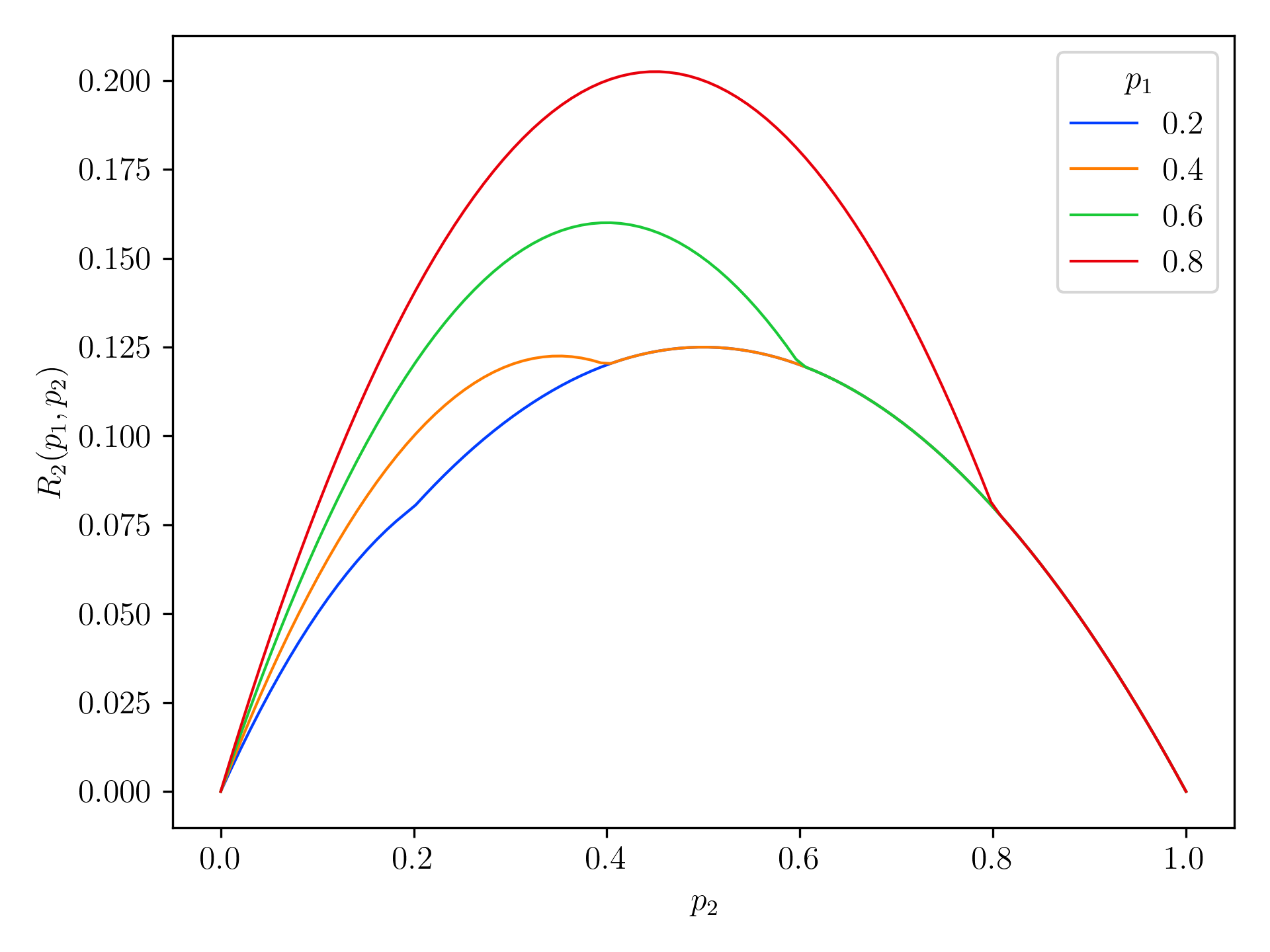
Figure 1: Plot of $R_{2}(p_{1},p_{2})$, for different values of $p_{1}$, when customers satisfice in a duopoly. Here we assume an equal proportion of customers prefer seller 1 to seller 2 (and vice versa), and $w_{c}\sim\textup{Unif}[0,1]$. This induces a revenue function $R_{2}(p_{1},p_{2})=p_{2}\left(\frac{1}{2}(1-p_{2})+\frac{1}{2}(p_{1}-p_{2})^{+}\right)$ for seller 2. Observe that $R_{2}(p_{1},p_{2})$ is nonsmooth. Moreover, for $p_{1}=0.4$, it has two local maxima: one at 0.5 and one at 0.35.

4.2 Structural characterization of local Nash equilibria

Having defined our main solution concept, we now turn to the question of tractably computing LNE under CLC choice. The following property, which we call the pseudo-competitive property, drives the majority of our results. Under this property, the revenue of a seller priced at $p$ remains unchanged if any seller pricing below $p$ changes its price to $p^{\prime}<p$. We define some additional notation to formalize this. Given price vector $\mathbf{p}$ and price $x$, let $\mathcal{S}_{\mathbf{p}}(x)=\left\{i\in\mathcal{N}\mathrel{\mathop{\mathchar 58\relax}}\,p_{i}\geq x\right\}$ be the set of sellers whose price is at least $x$. For $\mathcal{S}\subseteq\mathcal{N}$, $\mathbf{p}^{\mathcal{S}}$ denotes the price vector in which the prices of all sellers in $\mathcal{S}$ are preserved, and those in $\mathcal{N}\setminus\mathcal{S}$ are set to $0$.

Definition 4.4 (Pseudo-Competitive Property).

The pseudo-competitive property holds if, for all $i\in\mathcal{N}$, and $\mathbf{p}$, $\mathbf{p}^{\prime}\in\mathcal{V}^{N}$ such that:

1. $\mathcal{S}_{\mathbf{p}}(p_{i})=\mathcal{S}_{\mathbf{p}^{\prime}}(p_{i})$, i.e., the same set of sellers price weakly above $p_{i}$ in $\mathbf{p}$ and $\mathbf{p}^{\prime}$, and

2. $p_{j}=p^{\prime}_{j}$ for all $j\in\mathcal{S}_{\mathbf{p}}(p_{i})$, i.e., these higher-priced sellers set the same prices in $\mathbf{p}$ and $\mathbf{p}^{\prime}$,

we have that $R_{i}(\mathbf{p})=R_{i}(\mathbf{p}^{\prime})$.

Our first main result establishes that the revenue functions arising from the CLC choice model satisfy this property. We defer its proof to Appendix A.2.

Theorem 4.5.

The pseudo-competitive property holds under any CLC choice model.

Having established this fact, we next define the notion of a valid price-order pair that will be used for our main structural result. For any subset $\mathcal{S}\subseteq\mathcal{N}$, we let $p^{\min}(\mathcal{S})=\min\{p_{j};j\in\mathcal{S}\}$ denote the lowest price amongst sellers in $\mathcal{S}$, where we adopt the convention that $p^{\min}(\phi)=\bar{v}$. For $i\in\mathcal{N}$, $\mathcal{S}\subseteq\mathcal{N}\setminus\{i\}$, the undercutting interval or undercutting region of seller $i$ relative to $\mathcal{S}$ refers to the interval $[0,p^{\min}(\mathcal{S})]$. We refer to $R_{i}(p,\mathbf{p}_{-i}^{\mathcal{S}})$ in the undercutting region $[0,p^{\min}(\mathcal{S})]$ as the undercutting revenue curve of seller $i$ relative to $\mathcal{S}$ (where the prices of all sellers not in $\mathcal{S}$ are set to $0$).

Definition 4.6 (Valid order-price pair).

A valid order-price pair (VOP) is a tuple $(\pi,\mathbf{p})$ consisting of an ordering of sellers $\pi\mathrel{\mathop{\mathchar 58\relax}}[N]\rightarrow\mathcal{N}$ (i.e., $\pi(i)$ is the seller in rank $i$), and prices $\mathbf{p}\in\mathcal{V}^{N}$ such that:

1. $0\leq p_{\pi(N)}\leq p_{\pi(N-1)}\leq\cdots\leq p_{\pi(1)}\leq\bar{v}$.

2. Let $\mathcal{S}_{1}$ be the empty set, denoted by $\phi$, and for $i\in\{2,\cdots,N\}$, let $\mathcal{S}_{i}=\{\pi(j)\mathrel{\mathop{\mathchar 58\relax}}j<i\}$ denote the sellers ranked higher than $i$ in $\pi$. For all $i$, $p_{\pi(i)}$ is a local maximum of $R_{\pi(i)}(p,\mathbf{p}^{\mathcal{S}_{i}}_{-\pi(i)})$ in the undercutting interval $[0,p^{\min}(\mathcal{S}_{i})]$. We call these prices valid with respect to $\pi$.

Computationally, a valid order-price pair is more tractable than a LNE. In particular, for any ordering of sellers, the corresponding valid prices can be determined by sequentially solving (according to the ordering) $N$ constrained single-agent optimization problems up to local optimality. Each optimization problem corresponds to a rank in the ordering where the correspondingly ranked seller computes its undercutting best response to the prices of sellers higher in the ordering, assuming that all other sellers ranked lower set their prices to be $0$. Our main structural result shows that any LNE under CLC choice must be a VOP.

Theorem 4.7.

Under CLC choice, a price vector $\mathbf{p}$ is a LNE only if it belongs to a VOP.

In order to prove Theorem 4.7, we argue that, in any LNE, the local optimality of a seller’s price is preserved if any subset of sellers pricing weakly lower in that LNE reduced their price to 0. When sellers’ prices are distinct, this fact is implied by the pseudo-competitive property, i.e., a seller’s revenue is not impacted by the prices of strictly lower-priced sellers. The non-trivial aspect of the result is in showing that it holds even in LNE where sellers set equal prices, in which case the pseudo-competitive property fails to yield any meaningful implications (as it only pertains to strictly lower price changes). The result in this case leverages the structure of CLC choice. We defer its formal proof to Appendix A.3.

Theorem 4.7 has important implications for equilibrium computation under CLC choice. To elaborate further, we introduce a mild assumption of sellers’ undercutting revenue curves. For $i\in\mathcal{N}$, and $\mathbf{p}_{-i}\in\mathcal{V}^{N-1}$, $g_{i}(p_{i},\mathbf{p}_{-i})=\partial R_{i}(p,\mathbf{p}_{-i})/\partial p\big{|}_{p=p_{i}}$ is the partial derivative of $R_{i}(p,\mathbf{p}_{-i})$ with respect to $i$’s price. Similarly, for all $i\in\mathcal{N}$, $\mathcal{S}\subseteq\mathcal{N}\setminus\{i\}$ and $\mathbf{p}_{-i}\in\mathcal{V}^{N-1}$, such that $p^{\min}(\mathcal{S})>0$, we define $g_{i}(p_{i},\mathbf{p}_{-i}^{\mathcal{S}})=\partial R_{i}(p,\mathbf{p}_{-i}^{\mathcal{S}})/\partial p\big{|}_{p=p_{i}}$. We assume that this partial derivative exists for all $p_{i}\in[0,p^{\min}(\mathcal{S}))$, and make the following assumption.

Assumption 1 (Unimodality of undercutting revenue curves).

For all $i\in\mathcal{N}$, $\mathcal{S}\subseteq\mathcal{N}\setminus\{i\}$ and $\mathbf{p}_{-i}\in\mathcal{V}^{N-1}$, such that $p^{\min}(\mathcal{S})>0$, $R_{i}(p,\mathbf{p}_{-i}^{\mathcal{S}})$ is unimodal in the undercutting region, i.e., if $g_{i}(p,\mathbf{p}_{-i}^{\mathcal{S}})\leq 0$ for some $p\in[0,p^{\min}(\mathcal{S}))$, then $g_{i}(p^{\prime},\mathbf{p}_{-i}^{\mathcal{S}})<0$ for all $p^{\prime}\in(p,p^{\min}(\mathcal{S}))$.

1 enforces the mild condition that if a local optimum exists in the undercutting region for a seller, it must be unique. (Note that we assume unimodality of the revenue curve of a seller only in the undercutting region relative to the prices of the set of sellers $\mathcal{S}$. This assumption still allows for multiple local optima over $[0,\bar{v}]$.) We present examples for which 1 holds in Section 4.2.1.

Under 1, Theorem 4.7 implies that enumerating all LNE (and thus GNE) is computationally tractable when the number of sellers is small. (In contrast, computing GNE is generally intractable, even in two-player bimatrix games (Daskalakis et al.,, 2009).) This is because one can compute all valid order-price pairs, each of which requires solving a sequence of unimodal optimization problems, and then performing a computationally easy check for whether each of these is a LNE (or a GNE). We formalize this in Corollary 4.8, deferring its proof to Appendix A.4.

Corollary 4.8.

Under Assumption 1, there exists a computational procedure that:

1. finds all LNE, or determines that none exists, in $\textup{O}(N\cdot N!)$ undercutting best response computations;

2. finds all GNE, or determines that none exists, in $\textup{O}(N^{2}\cdot N!)$ undercutting best response computations.

Moreover, each of the undercutting best response computations in these procedures is a single-dimensional unimodal maximization problem.

The factorial dependence on the number of sellers in our procedure results from the exhaustive search over all seller orderings and the corresponding valid prices (if they exist). This dependence is inevitable in the worst case, even if the goal is to find a single LNE/GNE. This is because there could be exactly one LNE corresponding to an ordering that is a priori unknown, and which may take $O(N!)$ iterations to discover. Moreover, in the case where a LNE does not exist, an exhaustive search over all orderings is unavoidable to discover this. Hence, in the remainder of this section we turn to the task of finding sufficient conditions on the CLC class such that (i) a LNE is guaranteed to exist, and (ii) computing a LNE is polynomial in $N$. We present such a condition in 2.

Assumption 2 (Gradient dominance).

For two sellers $i,j\in\mathcal{N}$, seller $i$ gradient-dominates seller $j$ if for all $\mathbf{p}_{-\{i,j\}}\in\mathcal{V}^{N-2}$, and $p\in(0,\bar{v})$:

$$g_{i}(p_{i}=p,p_{j}=0,\mathbf{p}_{-\{i,j\}}) >\lim_{q\uparrow p}g_{j}(p_{i}=p,p_{j}=q,\mathbf{p}_{-\{i,j\}}).$$ (1)

Under gradient dominance, either $i$ gradient-dominates $j$ or $j$ gradient-dominates $i$, for all $i,j\in\mathcal{N}$.

We say that weak gradient dominance holds if this inequality holds for all price vectors in which a seller setting a positive price makes strictly positive revenue. (We call such price vectors non-trivial.)

At a high level, gradient dominance models settings in which one seller has a competitive strength relative to another due to, e.g., quality differences. We defer examples of CLC models for which gradient dominance holds to Section 4.2.1, and establish the connection between gradient dominance and existence and tractability of LNE in Proposition 4.9, whose proof we defer to Appendix A.5.

Proposition 4.9.

Under Assumptions 1 and 2, there exists a LNE $\mathbf{p}^{*}$ in which all prices are distinct, with $p_{i}^{*}>p_{j}^{*}$ for all sellers $i,j$ such that $i$ gradient-dominates $j$. Moreover, there exists a procedure that computes such a LNE in $O(N^{2})$ iterations, assuming knowledge of the gradient dominance relation for every pair of sellers.

We next present special cases of the CLC class for which gradient dominance holds, in particular highlighting the connection between gradient dominance and the strength of a seller along a non-price attribute.

4.2.1 Gradient Dominance: Special Cases

We first show that gradient dominance weakly holds under Best-I-Can-Afford behavior, allowing us to leverage Proposition 4.9 to characterize all non-trivial LNE for this special case. Recall, under BICA behavior, the customer chooses the highest-quality seller whose price is at most her willingness-to-pay. Let $q_{i}$ denote the quality of seller $i$, for $i\in\mathcal{N}$.

Proposition 4.10.

Under BICA behavior, for any two sellers $i,j\in\mathcal{N}$ with qualities $q_{i}>q_{j}$, seller $i$ weakly gradient-dominates seller $j$. Moreover, if all sellers’ qualities are distinct and customers’ willingness-to-pay distribution has a monotone hazard rate (MHR), there exists a unique non-trivial LNE in which sellers’ prices are strictly increasing in their respective qualities.

We defer the proof of Proposition 4.10 to Appendix A.6.1. While gradient dominance (weakly) holds for budgeted, purely quality-sensitive customers, we anticipate that it is robust to the presence of a limited number of price-sensitive customers. To formalize this intuition, we derive general sufficient conditions (i.e., beyond BICA behavior) for gradient dominance to hold in a duopoly.

For any customer $c$, let $\overline{\mathcal{N}}_{c}$ denote the consideration set formed without accounting for the willingness-to-pay constraint, i.e., $\overline{\mathcal{N}}_{c}=\{i\in\mathcal{N}\mathrel{\mathop{\mathchar 58\relax}}(v^{1}_{i},\ldots,v^{K}_{i})\in\mathcal{Y}_{c}\}.$ For $i,j\in\mathcal{N}$, we use $\overline{\lambda}_{{i}\succ{j}}$ to denote the probability that a customer strictly prefers $i$ to $j$ due to a non-price attribute ranked higher than price, conditional on the event $\overline{\mathcal{N}}_{c}=\{1,2\}$.

Proposition 4.11.

Consider a duopoly in which customers’ willingness-to-pay distribution is independent of all other CLC choice primitives, and has a monotone hazard rate. Then, seller $i$ gradient-dominates seller $j$ if and only if the following hold:

1. Non-price attribute dominance of seller $i$:

   $$\overline{\lambda}_{{i}\succ{j}}\mathbb{P}\left(\overline{\mathcal{N}}_{c}=\{1,2\}\right)+\mathbb{P}\left(\overline{\mathcal{N}}_{c}=\{i\}\right)>\left(1-\overline{\lambda}_{{i}\succ{j}}\right)\mathbb{P}\left(\overline{\mathcal{N}}_{c}=\{1,2\}\right)+\mathbb{P}\left(\overline{\mathcal{N}}_{c}=\{j\}\right)$$

2. Relative competitiveness of seller $j$:

   $$\left(1-\overline{\lambda}_{{i}\succ{j}}\right)\mathbb{P}\left(\overline{\mathcal{N}}_{c}=\{1,2\}\right)+\mathbb{P}\left(\overline{\mathcal{N}}_{c}=\{j\}\right)\geq\mathbb{P}\left(\overline{\mathcal{N}}_{c}=\{i\}\right)$$

Under these two conditions, there exists a LNE in which $p_{i}^{*}>p_{j}^{*}$.

Hence, we obtain robustness of gradient dominance to price-sensitive customers for BICA choice in Corollary 4.12 below. For notational convenience we assume that $q_{1}>q_{2}$.

Corollary 4.12.

Consider a duopoly composed of a mixture of BICA and greedy customers, with common willingness-to-pay distribution with monotone hazard rate. Then, seller 1 gradient-dominates seller 2 if strictly more than half of the customer population is of BICA type. In this case, there exists a LNE in which $p_{1}^{*}>p_{2}^{*}$.

We provide some intuition as to how the two conditions in Proposition 4.11 yield gradient dominance, deferring its proof to Appendix A.6.2. Condition 1 ensures that $i$ does not have a large incentive to undercut seller $j$ (i.e., that $i$ is “dominant” in the market). This occurs if more customers prefer $i$ to $j$ based on the following criteria: either only $i$ satisfies the non-price attribute criteria in the filtering phase, or $i$ beats $j$ on a non-price attribute ranked higher than price. Condition 2, on the other hand, ensures that not too many customers choose $i$ regardless of $p_{j}$. This guarantees that $j$ has an incentive to undercut $i$, and occurs if there are more customers who prefer $j$ to $i$ than customers for whom only $i$ survives the non-price filter.

Remark 4.13.

Distinctness of prices in equilibrium may seem particularly surprising given the fact that, under CLC choice, all customers prefer lower-priced items once they arrive at the price attribute in the selection phase. The above examples, however, recover the well-established intuition that quality sensitivity of customers plays a strong role in different prices arising in equilibrium. On the other hand, when the customer population is largely price-sensitive, gradient dominance likely fails to hold, and one would expect $\epsilon$-undercutting to be optimal for sellers, which would then lead to a price war. It is worth noting, however, that equal pricing at 0 cannot be a LNE if any positive mass of customers chooses based on a non-price attribute ranked higher than price (since a seller always stands to gain by setting a strictly positive price).

4.2.2 Non-equivalence of LNE and VOPs

Given Theorem 4.7, a natural question that arises is whether a VOP is necessarily a LNE. By the pseudo-competitive property, if all prices in a VOP are distinct, the corresponding price vector is necessarily a LNE. The issue then arises for VOPs in which two sellers price equally. To see this, consider a VOP $(\pi,\mathbf{p})$ in which two sellers $\pi(i)$ and $\pi(i+1)$ price equally. For this VOP to be a LNE, it must be the case that the local optimality of $p_{\pi(i)}$ is not perturbed when $\pi(i+1)$ raises its price from 0 to $p_{\pi(i)}$. Proposition 4.14 establishes that there exist settings for which this local optimality may indeed be perturbed; as a result, the converse of Theorem 4.7 does not hold in general. We defer its proof to Appendix A.7.

Proposition 4.14.

There exist instances of CLC choice for which a VOP is not a LNE.

5 Algorithmic price competition

For a platform that has access fine-grained customer choice data, it may be possible to estimate a CLC choice model and compute the resulting price equilibria using the insights derived in Section 4. However, since individual sellers on platforms do not have access to such data in general, the question of whether and how LNE arise in practice remains. In this section, we investigate whether natural price-update dynamics converge to a LNE under such cases. Having established existence of LNE under gradient dominance, we first theoretically study convergence for this subclass of choice models. We subsequently investigate robustness of our findings via extensive numerical experiments.

5.1 Convergence of distributed gradient ascent dynamics under gradient dominance

We analyze the distributed gradient ascent (GA) algorithm (Boyd and Vandenberghe,, 2004), formally presented in Appendix B.1. In this algorithm, at each timestep sellers take a step in the direction of the partial gradient of their respective revenue functions (assuming all other prices are fixed).

Additional notation and assumptions. For $i\in\mathcal{N}$, recall that $g_{i}(p_{i},\mathbf{p}_{-i})=\partial R_{i}(p,\mathbf{p}_{-i})/\partial p\big{|}_{p=p_{i}}$ denotes the partial derivative of $R_{i}(p,\mathbf{p}_{-i})$, assuming it exists. For $\mathcal{S}\subseteq\mathcal{N}\setminus\{i\}$, we denote by $p_{i}^{*}(\mathbf{p}_{-i}^{\mathcal{S}})\in\arg\max_{p\in[0,p^{\min}(\mathcal{S}))}R_{i}(p,\mathbf{p}_{-i}^{\mathcal{S}})$ an optimal price of seller $i$ in the open undercutting region relative to the set of sellers $\mathcal{S}$. When we say that $p_{i}^{*}(\mathbf{p}_{-i}^{\mathcal{S}})$ exists, we mean that the supremum is attained at $p_{i}^{*}(\mathbf{p}_{-i}^{\mathcal{S}})$. If the supremum is not attained, we use the convention that $p_{i}^{*}(\mathbf{p}_{-i}^{\mathcal{S}})=\infty$. Finally, we say that a price vector $\mathbf{p}$ is aligned with ordering $\pi$ if $p_{\pi(1)}>p_{\pi(2)}>\ldots>p_{\pi(N)}$. We will often abuse notation and let $\pi(1\mathrel{\mathop{\mathchar 58\relax}}l)$ denote the set of sellers in rank $1$ to $l$ for $l\in[N]$. We additionally let $\pi(1\mathrel{\mathop{\mathchar 58\relax}}0)$ be the empty set $\phi$, and define $p_{\pi(0)}=\bar{v}$. The following assumptions are required for our convergence result.

Assumption 3 (Regularity of undercutting revenue curves).

The following holds for all $i\in\mathcal{N}$, $\mathcal{S}\subseteq\mathcal{N}\setminus\{i\}$ and $\mathbf{p}_{-i}\in\mathcal{V}^{N-1}$.

1. Uniform boundedness of partial gradients: There exists a finite constant $G>0$ such that $|g_{i}(p,\mathbf{p}_{-i})|\leq G$ for all $p\in\mathbb{R}$.

2. Smoothness: $g_{i}(p,\mathbf{p}_{-i}^{\mathcal{S}})$ is continuous for all $p\in[0,p^{\min}(\mathcal{S}))$. Moreover, for all $i\in\mathcal{N}$, if $\mathbf{p}$ and $\mathbf{q}$ are aligned with the same ordering, there exists $L>0$ such that $|g_{i}(\mathbf{p})-g_{i}(\mathbf{q})|\leq L\|\mathbf{p}-\mathbf{q}\|_{1}.$

3. Strong unimodality: There exists a finite constant $K>0$ such that

   $$|g_{i}(p,\mathbf{p}_{-i}^{\mathcal{S}})|\geq K|p-\min\{p_{i}^{*}(\mathbf{p}_{-i}^{\mathcal{S}}),p^{\min}(\mathcal{S})\}|\quad\forall\,p\in[0,p^{\min}(\mathcal{S})).$$ (2)

4. No vanishing gradient below a partial VOP: Consider any ordering $\pi$, rank $l\in[N]$, and partial valid-order price pair $(\pi,\mathbf{p})$ that satisfies:

   $$p_{\pi(l^{\prime})}\mathrel{\mathop{\mathchar 58\relax}}=\arg\max_{0\leq p\leq p_{\pi(l^{\prime}-1)}}R_{\pi(l^{\prime})}(p,\mathbf{p}_{-\pi(l^{\prime})}^{\pi(1\mathrel{\mathop{\mathchar 58\relax}}l^{\prime}-1)})\quad\textrm{for }l^{\prime}\in\{1,\ldots,l\}.$$

   If the supremum is not attained in the problem $\sup_{0\leq p<p_{\pi(l)}}R_{\pi(l+1)}(p,\mathbf{p}_{-\pi(l+1)}^{\pi(1\mathrel{\mathop{\mathchar 58\relax}}l)})$, then

   $$\lim_{p\uparrow p_{\pi(l)}}g_{\pi(l+1)}(p,\mathbf{p}_{-\pi(l+1)}^{\pi(1\mathrel{\mathop{\mathchar 58\relax}}l)})>0.$$ (3)

Conditions 1 to 3 in 3 are common in much of the optimization literature on the convergence of gradient ascent and its variants (see, e.g., Broadie et al., (2011)). One can verify that these conditions hold as long as customers’ willingness-to-pay distribution conditioned on the other primitives of CLC choice has a Lipschitz continuous probability density function and a monotone hazard rate.

Condition 4 states that, if a seller’s supremum isn’t attained when all higher-priced sellers are at their respective local optima, its gradient does not vanish on approaching the next higher-priced seller from below. We claim that such an occurrence would be pathological, thus making this condition mild. To see this, we provide an example wherein a seller’s gradient does vanish at a partial VOP. Consider a duopoly in which customers only include one of two sellers in their consideration set, and purchase the item if their preferred seller’s price is below their willingness-to-pay. In this case, if the willingness-to-pay distribution is MHR and identical for all customers, then the sellers’ optimal price is unique and identical. As a result, the gradient of any seller’s revenue curve as its price approaches its competitor’s optimal price from below vanishes. More generally, one would expect Condition 4 to fail to hold in settings for which two sellers do not compete over the same market share, but their respective customer pools have otherwise identical choice primitives.

With these assumptions in hand, we state our convergence result.

Theorem 5.1.

Under Assumptions 2 and 3, a LNE with distinct prices exists. If moreover the learning rate schedule under distributed GA (Algorithm 1) is such that $\lim_{T\to\infty}\sum_{t=1}^{T}\eta_{t}^{2}<\infty$ and $\lim_{T\to\infty}\sum_{t=1}^{T}\eta_{t}=\infty$, sellers’ prices converge almost surely to a LNE.

We provide a proof sketch of Theorem 5.1, deferring its formal proof to Appendix B.2.

Proof sketch..

Existence of a LNE $\mathbf{p}^{*}$ in which sellers price distinctly follows from Proposition 4.9, since strong unimodality (Condition 3 in 3) implies 1. Let $\pi$ denote the ordering with which $\mathbf{p}^{*}$ is aligned.

Suppose first that sellers’ prices are aligned with $\pi$ for a large enough timestep. Since sellers’ revenue curves are invariant under strictly lower price changes, by Theorem 4.5, 3 implies that sellers will hierarchically converge to their respective undercutting optima.

Suppose now that the prices are aligned with an ordering $\pi^{\prime}\neq\pi$ for which a seller’s undercutting optimum is not attained. By Condition 5 of Assumption 3, this seller’s gradient doesn’t vanish as it approaches the boundary of its undercutting region. As a result, it will overtake the next higher price, thus ensuring that sellers exit out of this ordering.

Gradient dominance finally ensures that, when the stepsize is small enough, once the price dynamics exit an ordering, they cannot subsequently re-enter that ordering. Since the number of orderings is finite, they must eventually enter an ordering in which all sellers attain their undercutting optima. Hence, distributed GA eventually converges to a LNE. ∎

Theorem 5.1 establishes that, not only does gradient dominance guarantee existence of a LNE, but it also guarantees convergence to LNE under distributed gradient-based pricing (when coupled with standard regularity conditions on the individual revenue curves). In conjunction with the discussion of the practical validity of this condition in Section 4, this suggests that for CLC models in which a significant proportion of customers are quality-sensitive (e.g., BICA), one can expect frequent convergence to an equilibrium. We study this numerically in the following section.

5.2 Empirical analysis of gradient-driven price-update dynamics

Motivated by the fact that price and rating are two of the main attributes used for purchase decisions on e-commerce platforms, we consider price competition amongst $N\in\{2,\cdots,5\}$ sellers who differ on these two attributes. Given $N$, we assume that the quality of seller $i\in[N]$ is $q_{i}=i/N$.

Choice model. We assume that customers are either loyal or non-loyal. Loyal customers purchase from the seller to whom they are loyal as long as its price is at most their willingness-to-pay. Non-loyal customers are one of two types: quality-sensitive (QS) or price-sensitive (PS). QS and PS customers both form their consideration set based on a maximum willingness-to-pay and a minimum rating floor. However, they differ in the lexicographic choice phase: QS customers choose the highest-rated item in their consideration set, breaking ties based on price; PS customers, on the other hand, choose the cheapest item in their consideration set, breaking ties based on rating. QS and PS customers respectively generalize the BICA and CICT customers presented in Section 3.

We consider three settings for the distribution over these model primitives:

• Setting A: Customers are loyal, PS, or QS with an equal probability of $1/3$. A loyal customer is loyal to seller $i$ with probability $1/N$. The willingness-to-pay and rating floor for each customer (where applicable) is drawn independently from a $\textrm{Beta}(\alpha,\beta)$ distribution.

• Setting B: A customer is loyal with probability $1/3$ and non-loyal with probability $2/3$. A loyal customer is loyal to seller $i$ with probability $2i/(N(N+1))$, capturing the fact that higher-rated sellers have more loyal customers. The willingness-to-pay of a loyal customer is drawn from a $\textrm{Beta}(\alpha,\beta)$ distribution. Conditional on being non-loyal, the willingness-to-pay, rating floor, and probability of the customer being QS are all equal, and drawn from a $\textrm{Beta}(\alpha,\beta)$ distribution. This captures the reality that willingness-to-pay and quality sensitivity for non-loyal customers may be correlated, i.e., a higher willingness-to-pay may indicate a higher quality floor and a higher propensity to be quality-sensitive.

• Setting C: Same as Setting B, except that there are no loyal customers: all customers are non-loyal with probability $1$, with the same parameters.

Price dynamics. Sellers deploy distributed gradient-driven pricing schemes over a fixed time horizon $T=10^{4}\cdot N$. At the beginning of the horizon, we generate an initial set of prices independently and uniformly in $[0,1]$. To model the reality that sellers make price updates asynchronously, we choose a seller uniformly at random in each period to price experiment and subsequently make a price update. We assume that sellers implement the classical Kiefer-Wolfowitz algorithm for function optimization with zero-order feedback (Kiefer et al.,, 1952). Specifically, the chosen seller in each timestep observes a batch of $10^{3}$ customers, and randomly sets one of two prices for each customer in the batch: one above and one below its current incumbent price. The seller then estimates the gradient given the average revenue at each price and updates its incumbent price by taking a gradient-scaled step. Letting $c_{\tau}$ and $a_{\tau}$ respectively denote the finite difference width for gradient estimation and stepsize after $\tau$ updates, we let $c_{\tau}=1/\log\tau$ and $a_{\tau}=1/\tau$.

Observe that if the price trajectories converge to distinct prices under such a gradient-based pricing scheme, then it must be a LNE. We say that a price trajectory has converged if (i) for each seller, the difference between the maximum and minimum prices set in the last $10^{3}$ updates is within $1\%$ of the empirical average of the past $10^{3}$ prices, and (ii) the ordering of all prices remains unchanged in the last $10^{3}$ periods. If only (ii) is satisfied after $T$ periods, we say that the trajectory is order-convergent. When the price trajectory is only order-convergent, we expect prices to eventually converge due to the pseudo-competitive property, by the same arguments as those provided in the proof sketch of Theorem 5.1.

(a) Setting A

$(\alpha,\beta)$	$N$	C	OC
(1, 1)	2	100	100
(1, 1)	3	97	100
(1, 1)	4	97	100
(1, 1)	5	94	99
(0.5, 0.5)	2	100	100
(0.5, 0.5)	3	98	100
(0.5, 0.5)	4	93	100
(0.5, 0.5)	5	93	100
(2, 2)	2	100	100
(2, 2)	3	98	100
(2, 2)	4	91	100
(2, 2)	5	91	100
(2, 4)	2	99	100
(2, 4)	3	95	99
(2, 4)	4	91	100
(2, 4)	5	80	100
(4, 2)	2	98	100
(4, 2)	3	90	100
(4, 2)	4	84	100
(4, 2)	5	72	100

(b) Setting B

$(\alpha,\beta)$	$N$	C	OC
(1, 1)	2	99	100
(1, 1)	3	96	100
(1, 1)	4	98	100
(1, 1)	5	97	100
(0.5, 0.5)	2	100	100
(0.5, 0.5)	3	99	99
(0.5, 0.5)	4	98	100
(0.5, 0.5)	5	95	99
(2, 2)	2	100	100
(2, 2)	3	99	100
(2, 2)	4	98	100
(2, 2)	5	95	99
(2, 4)	2	100	100
(2, 4)	3	100	100
(2, 4)	4	99	99
(2, 4)	5	92	99
(4, 2)	2	100	100
(4, 2)	3	97	100
(4, 2)	4	95	99
(4, 2)	5	89	99

(c) Setting C

$(\alpha,\beta)$	$N$	C	OC
(1, 1)	2	99	100
(1, 1)	3	98	100
(1, 1)	4	98	100
(1, 1)	5	96	99
(0.5, 0.5)	2	98	100
(0.5, 0.5)	3	100	100
(0.5, 0.5)	4	96	100
(0.5, 0.5)	5	96	99
(2, 2)	2	100	100
(2, 2)	3	97	100
(2, 2)	4	93	100
(2, 2)	5	97	100
(2, 4)	2	100	100
(2, 4)	3	97	100
(2, 4)	4	96	99
(2, 4)	5	93	99
(4, 2)	2	99	100
(4, 2)	3	96	100
(4, 2)	4	91	100
(4, 2)	5	83	100

(d) Setting D

$(\alpha,\beta)$	$N$	C	OC	E
(1, 1)	2	99	100	97
(1, 1)	3	97	100	96
(1, 1)	4	99	100	97
(1, 1)	5	99	100	95
(0.5, 0.5)	2	100	100	91
(0.5, 0.5)	3	98	100	96
(0.5, 0.5)	4	98	100	95
(0.5, 0.5)	5	96	100	93
(2, 2)	2	100	100	93
(2, 2)	3	97	99	93
(2, 2)	4	99	100	90
(2, 2)	5	95	100	94
(2, 4)	2	100	100	95
(2, 4)	3	99	100	95
(2, 4)	4	95	99	93
(2, 4)	5	91	99	87
(4, 2)	2	99	100	96
(4, 2)	3	96	99	93
(4, 2)	4	88	99	85
(4, 2)	5	85	100	78

Table 1: Number of convergent (C) and order-convergent (OC) trajectories out of 100 random initializations in each setting

Results. Table 1 shows the number of replications out of $100$ random draws of initial prices that result in price and order convergence for Settings A-C. (Setting D shows a final set of robustness results, discussed at the end of the section.) We observe that the price dynamics converge in the majority of settings, with at least 72 convergent trajectories out of 100 in the worst case over all parameters in Setting A, 89 in Setting B, and 83 in Setting C. If we consider order-convergent trajectories, the numbers further improve, with at least 99 order-convergent trajectories in the worst case across all settings. Overall, our results suggest that LNE are frequently learnable via distributed gradient-driven pricing, under CLC models of practical interest.

We include sample non-order-convergent price trajectories in Figure 2. Two of the trajectories show sellers entering undercutting price wars as their prices approach each other (sellers 2-3 in Figure 2(a), and sellers 1-2 in Figure 2(c)). These undercutting price wars are due to the existence of price-sensitive customers who choose the cheapest item in their consideration set. Indeed, if all customers are price-sensitive, the only equilibrium is once in which all sellers price at zero. Again, these results underscore the idea that convergence arises in part due to the existence of quality-sensitive and loyal customers, who counteract the incentive to enter a price war.

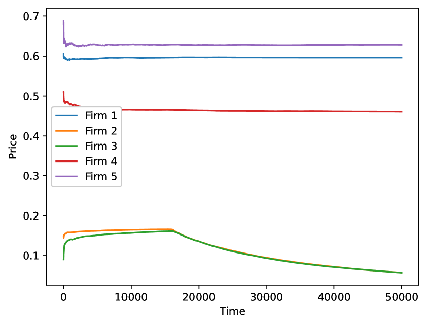
(a) Setting A: $\alpha=0.5,$ $\beta=0.5$

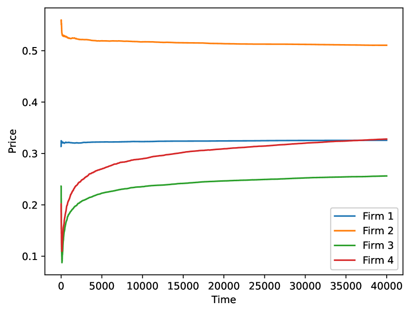
(b) Setting B: $\alpha=1,$ $\beta=1$

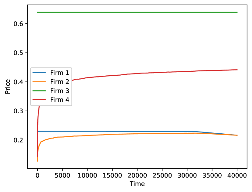
(c) Setting C: $\alpha=1,$ $\beta=1$

Figure 2: Sample non-convergent trajectories in Settings A-C

Robustness to non-CLC choice. We conclude our numerical experiments by investigating the robustness of these observations to non-CLC customers. Specifically, we modify Setting C such that 10% of customers behave according to the Multinomial Logit (MNL) choice model, with the remainder behaving as in Setting C. For an MNL customer, the utility of choosing a seller $i$ with rating $q$ and price $p$ is assumed to be $q-p+\epsilon$, where $\epsilon$ is an independent noise term with a Gumbel distribution with location parameter $0$ and scale parameter $1$. The customer chooses the seller with the highest utility. We refer to this setting as Setting D. We choose the same price initializations for each of the 100 trajectories for both Settings C and D, and study the impact of MNL customers both on convergence and on the limit points themselves.

Convergence results for Setting D are shown in Table 1. We obtain consistent convergence to a LNE (in at least 85 random draws, in the worst case), as well as order-convergence (in at least 99 draws, in the worst case). The column labeled “E” for Setting D shows the number of convergent trajectories such that (i) the corresponding trajectories in Setting C converge as well (we call these co-convergent trajectories), and (ii) the convergence point is within a tolerance of $10\%$ of the limit point under Setting C; this tolerance aligns with the fact that $10\%$ of the population is of the MNL type. We observe that trajectories under Settings C and D are almost always co-convergent, and that these convergence points are frequently close, with both conditions holding in at least 78 random draws, in the worst case. Overall, these observations suggest that our equilibrium insights are robust to the limited inclusion of well-studied utility-maximizing behaviors.

6 Conclusion

Motivated by the sorting and filtering capabilities of modern e-commerce platforms, we studied price competition under a hybrid model of customer behavior that tackles a two-fold objective: flexibly capturing sequential search and selection on these platforms, and being conducive to the tractable analysis of their induced equilibria. We identified two crucial properties, the pseudo-competitive property and gradient dominance, which render equilibria efficiently computable from the platform’s perspective, as well as efficiently learnable under distributed gradient-based dynamics. Overall, our work demonstrates that CLC is an attractive modeling framework for platforms to analyze and predict market outcomes.

While our work presents strong evidence for frequent convergence to local Nash equilibria of gradient-driven pricing, an interesting future direction would be to study equilibrium computation and learning past the gradient dominance condition. It would moreover be interesting to explore algorithms that provably yield convergence to other limit points of interest, such as global Nash equilibria (as opposed to local), and seller / customer surplus-maximizing prices.

Appendix A Section 4 Omitted Proofs

A.1 Proof of Proposition 4.1

Proof.

Consider first the special case of CLC choice in which all customers are greedy, i.e., they purchase from the cheapest seller, as long as their willingness-to-pay exceeds the price of the item. In this case, it is well-known that the unique equilibrium is one in which all sellers price at zero.

Consider now a duopoly wherein $1-\epsilon$ fraction of the population is greedy, and $\epsilon$ fraction is loyal, and only ever purchases from seller 1. Suppose moreover that the willingness-to-pay $w_{c}\sim\textup{Unif}[0,1]$. In this setting, no equilibrium exists. This follows from the fact that, for any strictly positive price $p$ set by seller 1, the best response of seller 2 is to set $p-\epsilon_{0}$, for arbitrarily small $\epsilon_{0}>0$ (i.e., the best response is not attained). However, it is never optimal for seller 1 to set a price of 0, given that $\epsilon$ fraction of customers will purchase its item at a strictly positive price.

Consider finally a duopoly in which customers are satisficers, with customers preferring seller 1 to seller 2 (and vice versa) with probability 1/2. Their willingness-to-pay for the item is drawn from the uniform distribution over $[0,1]$; they moreover purchase from the first seller for whom the price is (weakly) below their willingness-to-pay, inspecting sellers according to their preference. For this setting one can verify that there exist two equilibria, both defined by one seller pricing at 1/2, and the other pricing at 3/8. ∎

A.2 Proof of Theorem 4.5

Proof.

We argue this at the customer choice level. Consider a seller $i$ pricing at $p$ and suppose that a seller $j$ with $p_{j}<p$ changes its original price $p_{j}$ to some $p_{j}^{\prime}<p$. We show that this change does not impact whether or not seller $j$ is chosen by a customer; hence, it does not impact the revenue of seller $i$.

Note that the only customers who could possibly impact seller $i$’s revenue under this change are those for whom both $i$ and $j$ were in the consideration set when $j$ priced at $p_{j}$. To see this, consider first a customer who did not include $i$ in her consideration set under $p_{j}$. In this case, $i$ will continue to be excluded under $p_{j}^{\prime}$, and seller $i$ will continue to earn zero revenue from such a customer. Consider next a customer who included $i$ but not $j$ in her consideration set under $p_{j}$. Since $i$ was in the consideration set, the customer’s willingness-to-pay exceeds $p$, and $p_{j}$ as a result. Hence, $j$ must have been excluded due to a non-price attribute, and $j$ will continue to be excluded due to a non-price attribute under $p_{j}^{\prime}$. The choice outcome from the perspective of $i$ does not change in this case as well.

Consider finally customers who included both $i$ and $j$ in their consideration set under $p_{j}$. As argued above, since $i$ was in the consideration set under $p_{j}$, $w_{c}\geq p>p_{j}^{\prime}$, and thus both $i$ and $j$ remain in the consideration set under $p_{j}^{\prime}$. Now, under $j$’s old price, if the customer chose from the consideration set based on a non-price attribute ranked higher than price, she will continue to make the same choice under the new price. If she chose based on either the price attribute or some non-price attribute ranked lower than the price, then $i$ is not chosen before or after the price change, since its price is not the lowest in the consideration set under $p_{j}$ or $p_{j}^{\prime}$. In summary, the outcome of whether or not $i$ is chosen remains unchanged, which proves the result. ∎

A.3 Proof of Theorem 4.7

We first prove that the following property (which we refer to as cross-monotonicity) holds under CLC choice.

Proposition A.1.

Under CLC choice, for all $i\in\mathcal{N}$, $p_{i}\in\mathbb{R}$, $R_{i}(p_{i},\mathbf{p}_{-i})$ is non-decreasing in $\mathbf{p}_{-i}$, i.e., if $\mathbf{p}^{\prime}_{-i}\mathbf{\geq}\mathbf{p}_{-i}$ (component-wise), then $R_{i}(p_{i},\mathbf{p}^{\prime}_{-i})\geq R_{i}(p_{i},\mathbf{p}_{-i})$.

Proof.

Fix seller $i\in\mathcal{N}$, and suppose there exists a seller $j\in\mathcal{N}\setminus\{i\}$ that strictly increased its price to $p_{j}^{\prime}>p_{j}$. Note that this change only affects a customer $c$ such that $\{i,j\}\in\mathcal{N}_{c}$ for some $j\in\mathcal{S}$. Consider any customer $c$ for which this holds.

If $c$ had not chosen $i$ under $p_{j}$, then $i$’s revenue from $c$ is 0, and can only weakly increase after a price change of $j$. Thus, it suffices to argue that if $c$ chooses $i$, then they continue to choose $i$ after an increase in $p_{j}$, implying a weak increase in revenue for $i$.

If $c$ had previously chosen $i$ due to a non-price attribute ranked higher than price, then the price change of seller $j$ does not change her previous decision. Suppose now that $c$ chose $i$ based on either the price attribute, or an attribute ranked lower than the price. Then, it must be that $p_{i}\leq p_{j}<p_{j^{\prime}}$. In this case, even after the price increase in $p_{j}$, $c$ would continue to choose $i$. This is because the customer cannot choose $j$ after this change since $p_{i}<p_{j}^{\prime}$, and it cannot choose some other seller since if that were the case, then they would have chosen that seller under $p_{j}$ as well, contradicting the fact that $i$ was chosen under $p_{j}$. ∎

With this result in hand, we prove Theorem 4.7.

Proof of Theorem 4.7..

Suppose $\mathbf{p}$ is a LNE, and let $\pi$ denote an ordering induced by $\mathbf{p}$ (breaking ties arbitrarily).

Suppose first that all prices in $\mathbf{p}$ are distinct. Then, these prices are necessarily valid with respect to $\pi$ (i.e., $p_{\pi(i)}$ is a local optimum in the undercutting region of $\pi(i)$, for all $i$). This follows from the pseudo-competitive property: for any $i$, $R(p,\mathbf{p}_{-\pi(i)}^{\mathcal{S}_{i}})=R(p,\mathbf{p}_{-\pi(i)})$. Hence, the local optimality of a seller in the ordering is preserved even if the prices of lower-ranked sellers are reduced to $0$, implying the validity of these prices with respect to $\pi$.

Hence, it remains to consider the case where at least two prices in $\mathbf{p}$ are equal. Consider the first set of sellers with equal prices (i.e., those ranked highest in the ordering), and let $l$ denote the size of this set. We denote these sellers by $\{j_{0},\ldots,j_{l}\}$, with $j_{0},\ldots,j_{l}$ following the same order as $\pi$. By the same argument as the one used when all prices in $\mathbf{p}$ are distinct, the price of any seller ranked higher than $j_{0}$ is locally optimal with respect to $\mathbf{p}$. We argue that the local optimality of $p_{j_{0}}=\ldots=p_{j_{l}}$ is not perturbed.

Case 1: $p_{j_{0}}=p_{j_{1}}=\cdots=p_{j_{l}}=0.$

For any $j\in\{j_{0},\ldots,j_{l}\}$, $R_{j}(p_{j},\mathbf{p}_{-j})=R_{j}(p_{j},\mathbf{p}_{-j}^{S_{j}})=0$. Thus, if 0 is a local optimum for $j$ over $[0,\bar{v}]$, it is necessarily a local optimum over $j$’s relevant undercutting region.

Case 2: $p_{j_{0}}=p_{j_{1}}=\cdots=p_{j_{l}}>0.$

We will argue that $p_{j_{0}}$ is locally optimal over its relevant undercutting region if any $\mathcal{S}\subseteq\{j_{1},\cdots,j_{l}\}$ reduce their price to $0$. By symmetry, then, the same will hold true for any $j\in\{j_{0},\cdots,j_{l}\}$. Repeating this argument for the next set of equally priced sellers below $\{j_{0},\ldots,j_{l}\}$, until no equally priced sellers remain (or all sellers are priced at zero), we will obtain the theorem.

Lemma A.2 plays a key role in proving this claim. It establishes that sellers $j_{1},\ldots,j_{l}$ reducing their prices does not impact the expected revenue of $j_{0}$.

Lemma A.2.

$R_{j_{0}}(p,\mathbf{p}_{-j_{0}})=R_{j_{0}}(p,\mathbf{p}^{\prime}_{-j_{0}})$ for all $\mathbf{p}^{\prime}$ such that $p^{\prime}_{j_{i}}\leq p_{j_{i}}$, $i\in\{1,\ldots,l\}$.

Proof of Lemma A.2..

Consider the subset $\mathcal{S}\subseteq\{j_{1},\ldots,j_{l}\}$ for which $p_{j_{i}}^{\prime}<p_{j_{i}}$. As argued in the proof of Proposition A.1, for $j_{0}$ to be affected by this price decrease, it must be that there exists a customer $c$ such that $\{j_{0},j\}\subseteq\mathcal{N}_{c}$ for some $j\in\mathcal{S}$. For any such customer $c$, it moreover must have been that $j_{0}$ and $j$ were ranked equally on all attributes up until price, and that $c$ had chosen $j_{0}$ (else, $c$ chose $j$ both before and after the price change, resulting in no change in revenue for $j_{0}$).

Given this, since $j$ strictly decreased its price, all customers who chose $j_{0}$ based on an attribute $k$ ranked lower than price under $\mathbf{p}$, now choose $j$ under $\mathbf{p}^{\prime}$. We claim that this occurs for a measure 0 set of customers. To see this, suppose there existed $j\in\{j_{1},\ldots,j_{l}\}$ such that a strictly positive mass of customers chose $j_{0}$ over $j$ based on an attribute ranked lower than price. Then, $j$ would stand to gain a discrete mass of customers by infinitesimally undercutting $p_{j_{0}}$, thus contradicting the local optimality of $p_{j}=p_{j_{0}}$.

Since all but a measure 0 set of customers move their choice from $j_{0}$ to $j\in\mathcal{S}$ under this price change, the expected demand (and hence expected revenue) of $j_{0}$ is invariant to weakly lower price changes of $j_{1},\ldots,j_{l}$. ∎

We now leverage Lemma A.2 to show that $p_{j_{0}}$ remains locally optimal under any price vector $\mathbf{p}^{\prime}$ such that $p_{j_{i}}^{\prime}=0$ for some subset of sellers $\mathcal{S}\subseteq\{1,\ldots,l\}$. Lemma A.3 establishes that it is never optimal for $j_{0}$ to $\epsilon$-undercut its original price $p_{j_{0}}$ under $\mathbf{p}^{\prime}$.

Lemma A.3.

There exists $\epsilon_{0}>0$ such that, for all $0<\epsilon\leq\epsilon_{0}$, $R_{j_{0}}(p_{j_{0}}-\epsilon,\mathbf{p}^{\prime}_{-j_{0}})\leq R_{j_{0}}(p_{j_{0}},\mathbf{p}^{\prime}_{-j_{0}})$.

Proof of Lemma A.3..

By local optimality of $p_{j_{0}}$ under $\mathbf{p}$, there exists $\epsilon_{0}>0$ such that for $0<\epsilon\leq\epsilon_{0}$:

$$0 \leq R_{j_{0}}(p_{j_{0}},\mathbf{p}_{-j_{0}})-R_{j_{0}}(p_{j_{0}}-\epsilon,\mathbf{p}_{-j_{0}})$$ (4)

$$\leq R_{j_{0}}(p_{j_{0}},\mathbf{p}_{-j_{0}})-R_{j_{0}}(p_{j_{0}}-\epsilon,\mathbf{p}^{\prime}_{-j_{0}})$$ (5)

$$=R_{j_{0}}(p_{j_{0}},\mathbf{p}^{\prime}_{-j_{0}})-R_{j_{0}}(p_{j_{0}}-\epsilon,\mathbf{p}^{\prime}_{-j_{0}}).$$ (6)

Here, (5) follows from cross-monotonicity (Proposition A.1), and (6) follows from Lemma A.2. ∎

We conclude the proof by establishing that it is never optimal for $j_{0}$ to $\epsilon$-overcut $p_{j_{0}}$ under $\mathbf{p}^{\prime}$.

Lemma A.4.

There exists $\epsilon_{0}>0$ such that, for all $0<\epsilon\leq\epsilon_{0}$, $R_{j_{0}}(p_{j_{0}}+\epsilon,\mathbf{p}^{\prime}_{-j_{0}})\leq R_{j_{0}}(p_{j_{0}},\mathbf{p}^{\prime}_{-j_{0}})$.

Proof of Lemma A.4..

By local optimality of $p_{j_{0}}$ under $\mathbf{p}$, there exists $\epsilon_{0}>0$ such that, for all $0<\epsilon\leq\epsilon_{0}$:

$$0 \leq R_{j_{0}}(p_{j_{0}},\mathbf{p}_{-j_{0}})-R_{j_{0}}(p_{j_{0}}+\epsilon,\mathbf{p}_{-j_{0}})$$ (7)

$$=R_{j_{0}}(p_{j_{0}},\mathbf{p}_{-j_{0}})-R_{j_{0}}(p_{j_{0}}+\epsilon,\mathbf{p}^{\prime}_{-j_{0}})$$ (8)

$$=R_{j_{0}}(p_{j_{0}},\mathbf{p}^{\prime}_{-j_{0}})-R_{j_{0}}(p_{j_{0}}+\epsilon,\mathbf{p}^{\prime}_{-j_{0}}).$$ (9)

Here, (8) follows from the pseudo-competitive property, and (9) follows from Lemma A.2. Thus, increasing its price is not locally beneficial to $j_{0}$ under price vector $\mathbf{p}^{\prime}$. ∎

Putting Lemma A.3 and Lemma A.4 together, the local optimality of $p_{j_{0}}$ is preserved under any such $\mathbf{p}^{\prime}$. ∎

A.4 Proof of Corollary 4.8

For notational convenience, for $p\in\mathcal{V}$, we let $M_{i}(p)=R_{i}(p,\mathbf{p}^{\phi}_{-i})$). We refer to $M_{i}(\cdot)$ as the loyalist revenue curve, informally referring to the fact that it is the revenue obtained from customers who only purchase from $i$, regardless of other sellers’ prices.

Proof.

The proof is constructive. Let $\pi$ denote an arbitrary ordering over sellers.

Initialization. Fix an arbitrary $\pi$, mark it as inspected, and proceed to Phase 1 below.

Phase 1: Valid order-price pair computation. Compute the VOP associated with $\pi$ (see Definition 4.6). If a corresponding VOP exists, let $\mathbf{p}$ denote the resulting price vector, and proceed to Phase 2. Else, choose a new, uninspected ordering. Mark this new ordering as inspected, and go back to the beginning of Phase 1.

Phase 2: LNE / GNE verification. For $i\in[N]$, compute:

$$\max\left\{\sup_{p\in[p_{\pi(i)},p_{\pi(i-1})]}R_{\pi(i)}(p,\mathbf{p}_{-\pi(i)}),\sup_{p\in[p_{\pi(i+1)},p_{\pi(i)}]}R_{\pi(i)}(p,\mathbf{p}_{-\pi(i)})\right\}.$$

If this quantity strictly exceeds $R_{\pi(i)}(\mathbf{p})$ for some $i\in[N]$, then $\mathbf{p}$ is not a LNE (and hence, not a GNE); else, it is a LNE.

If $\mathbf{p}$ is a LNE, verify that it is a GNE by computing for $i\in[N]$, $j\in[N]\setminus\{i\}$

$$\begin{cases}\sup_{p\in[p_{\pi(j)},p_{\pi(j-1)}]}R_{\pi(i)}(p,\mathbf{p}_{-\pi(i)})\quad\text{if }j<i\text{ or }j>i+1\\ \sup_{p\in[p_{\pi(i+1)},p_{\pi(i-1)}]}R_{\pi(i)}(p,\mathbf{p}_{-\pi(i)})\quad\text{if }j=i+1.\end{cases}$$

If for $i\in[N]$, any of these revenues is strictly higher than $R_{\pi(i)}(\mathbf{p})$, then $\mathbf{p}$ is not a GNE; else, it is. Choose a new, uninspected ordering, mark it as inspected, and proceed to the beginning of Phase 1. If all $N!$ orderings have been traversed, either output all identified LNE/GNE, or return that none exists.

Correctness and termination. By the unimodality assumption, for each ordering $\pi$ there exists at most one VOP pair $(\pi,\mathbf{p})$. Hence, by Theorem 4.7, if a LNE exists, it must have been found in Phase 1. Since a GNE is a LNE, it must also have been found in Phase 1, if it exists. Phase 2 is a simple consistency check to see if the local optimum computed for each seller is locally / globally optimal with respect to $\mathbf{p}$.

We conclude the proof by giving an upper bound on the number of undercutting best-response computations required for the procedure to terminate. For each ordering (of which there are $N!$), at most $N$ undercutting best-response computations are performed during Phase 1. Verifying whether each of these VOPs is a LNE requires an additional two best-response computations per seller, per ordering. This yields the upper bound on the number of best-response computations to find all LNE, or to find that none exists.

The second GNE verification phase requires at most $N$ undercutting best-response computations per seller, for a given LNE. This then yields the $\textup{O}(N^{2})$ best-response computations across all sellers.

The bound in Part 2 of the statement follows from putting these two together. Namely, each ordering requires at most $N^{2}+N$ local best-response computations to check if the LNE is a GNE. Doing this for all $N!$ orderings give rise to an upper bound of $\textup{O}((N^{2}+N)N!)$ undercutting best-response computations. ∎

A.5 Proof of Proposition 4.9

We first introduce some useful terminology. If seller $i$ gradient-dominates seller $j$ and $p_{i}>p_{j}$, we say that sellers $i$ and $j$ are correctly ordered. Otherwise, $i$ and $j$ are said to be incorrectly ordered. The following fact emerges as a consequence of gradient dominance.

Lemma A.5.

Under gradient dominance, there exists an ordering $\pi$ such that, for all $\mathbf{p}\in\mathcal{V}^{N}$ aligned with $\pi$ such that $p_{\pi(N)}>0$ and all $l\in[N-1]$:

$$g_{\pi(l)}\left(p_{\pi(l)},\mathbf{p}_{-\pi(l)}^{\pi(1\mathrel{\mathop{\mathchar 58\relax}}l-1)}\right) >\lim_{p\uparrow p_{\pi(l)}}g_{\pi(l+1)}\left(p,\mathbf{p}_{-\pi(l+1)}^{\pi(1\mathrel{\mathop{\mathchar 58\relax}}l)}\right).$$ (10)

Proof.

The proof is constructive. Consider any ordering $\pi$ such that (10) does not hold, and let $l^{*}$ denote the first rank in the ordering such that $\exists\,\mathbf{p}\in\mathcal{V}^{N}$ such that

$$g_{\pi(l)}\left(p_{\pi(l)},\mathbf{p}_{-\pi(l)}^{\pi(1\mathrel{\mathop{\mathchar 58\relax}}l-1)}\right)\leq\lim_{p\uparrow p_{\pi(l)}}g_{\pi(l+1)}\left(p,\mathbf{p}_{-\pi(l+1)}^{\pi(1\mathrel{\mathop{\mathchar 58\relax}}l)}\right)$$,

with $p_{\pi(N)}>0$. By gradient dominance, then, $g_{\pi(l+1)}\left(p_{\pi(l+1)},\mathbf{p}_{-\pi(l+1)}^{\pi(1\mathrel{\mathop{\mathchar 58\relax}}l)}\right)>\lim_{p\uparrow p_{\pi(l+1)}}g_{\pi(l)}\left(p,\mathbf{p}_{-\pi(l)}^{\pi(1\mathrel{\mathop{\mathchar 58\relax}}l-1)}\right)$ for all $\mathbf{p}\in\mathcal{V}^{N}$ such that $p_{\pi(N)}>0$. Define $\pi^{\prime}$ that flips the two incorrectly ordered sellers, i.e.:

$$\begin{cases}\pi^{\prime}(l)&=\pi(l)\quad\forall\ l\in[N]\setminus\{l^{*},l^{*}+1\}\\ \pi^{\prime}(l^{*})&=\pi(l^{*}+1)\\ \pi^{\prime}(l^{*}+1)&=\pi(l^{*}).\end{cases}$$

Repeat this process with $\pi^{\prime}$, as long as there exist incorrectly ordered sellers in the newly generated ordering $\pi^{\prime}$. To see why this process must terminate with all sellers correctly ordered, note that, once two sellers have been swapped, by gradient dominance they will never be swapped again. Thus the algorithm never revisits the same ordering. Since there are finitely many orderings and, for each ordering, finitely many pairs to potentially swap, this algorithm must terminate in an ordering $\pi$ such that (10) holds. ∎

We use this fact to establish existence of LNE.

Proof of Proposition 4.9..

For $\mathcal{S}\subseteq\mathcal{N}\setminus\{i\}$, let $p_{i}^{*}(\mathbf{p}_{-i}^{\mathcal{S}})\in\arg\max_{p\in[0,p^{\min}(\mathcal{S}))}R_{i}(p,\mathbf{p}_{-i}^{\mathcal{S}})$ denote the unique optimal price of seller $i$ in the open undercutting region relative to the set of sellers $\mathcal{S}$. (Uniqueness follows from 1.)

We first argue that $p_{i}^{*}(\mathbf{p}_{-i}^{\mathcal{S}})\neq 0$, if it exists. Suppose for contradiction that $p_{i}^{*}(\mathbf{p}_{-i}^{\mathcal{S}})=0$. Since $R_{i}(0,\mathbf{p}_{-i}^{\mathcal{S}})=0$, the optimal revenue is $0$, which implies that $R_{i}(p,\mathbf{p}_{-i}^{\mathcal{S}})=0$ for all $p\in[0,p^{\min}(\mathcal{S})]$, contradicting the unimodality assumption. Thus, $p_{i}^{*}(\mathbf{p}_{-i}^{\mathcal{S}})\in(0,p^{\min}(\mathcal{S}))$, and $g_{i}(p_{i}^{*}(\mathbf{p}_{-i}^{\mathcal{S}}),\mathbf{p}_{-i}^{\mathcal{S}})=0$.

Now, let $\pi$ be such that (10) holds, and define $p^{*}_{\pi(1)}=\arg\max_{p}R_{\pi(1)}(p,\mathbf{p}^{\phi}_{-i})$. Using similar arguments as above, $p^{*}_{\pi(1)}\in(0,\bar{v})$, and $g_{\pi(1)}(p^{*}_{\pi(1)},\mathbf{p}_{-\pi(1)}^{\phi})=0$. By (10), we then have

$$\lim_{p\uparrow p_{\pi(1)}}g_{\pi(2)}\left(p,\mathbf{p}_{-\pi(2)}^{\pi(1)}\right)<g_{\pi(1)}(p_{\pi(1)}^{M},\mathbf{p}_{-\pi(1)}^{\phi})=0.$$

By 1, then, $R_{\pi(2)}(\cdot,\mathbf{p}_{-\pi(2)}^{\pi(1)})$ attains its unique maximum $p_{\pi(2)}^{*}$ in $(0,p_{\pi(1)}^{*})$, with
$g_{\pi(2)}\left(p_{\pi(2)}^{*},\mathbf{p}_{-\pi(2)}^{\pi(1)}\right)=0$. Iterating this argument for $l=3,\ldots,N$, we obtain that $\mathbf{p}^{*}$ is a VOP with distinct prices, and hence a LNE.

Note that finding an ordering $\pi$ such that seller $i$ is ranked above seller $j$ if and only if $i$ gradient-dominates $j$ requires $O(N^{2})$ comparisons. Given $\pi$, it suffices to find the aligned price vector $\mathbf{p}^{*}$, which can be done in $O(N)$ computations. ∎

A.6 Gradient dominance: Special cases

In the remainder of this section, we let $F$ denote the cumulative distribution function of customers’ willingness-to-pay, and $f$ the corresponding density. For ease of notation we define $\bar{F}(\cdot)=1-F(\cdot)$.

A.6.1 Proof of Proposition 4.10

Proof.

We first argue that weak gradient dominance holds.

Consider $\mathbf{p}$ such that $p_{i}>p_{j}$. We consider two cases.

Case 1: There exists $k\in\mathcal{N}\setminus\{i,j\}$ such that $q_{k}>q_{i}$ and $p_{k}\leq p_{i}$. This is a trivial price configuration since no customer chooses $i$ (anyone who can afford $p_{i}$ can also afford $p_{k}$, and will choose this higher-rated seller). Hence, for any such price vector seller $i$ has a revenue of zero.

Case 2: $p_{k}>p_{i}$ for all $k\in\mathcal{N}$ such that $q_{k}>q_{i}$. We have:

$$R_{i}(p_{i},p_{j},\mathbf{p}_{-\{i,j\}})=p_{i}\cdot\mathbb{P}\left(p_{i}\leq w_{c}<\min_{k\mathrel{\mathop{\mathchar 58\relax}}q_{k}>q_{i}}p_{k}\right)$$

$$\implies g_{i}(p_{i},p_{j},\mathbf{p}_{-\{i,j\}})=\mathbb{P}\left(p_{i}\leq w_{c}<\min_{k\mathrel{\mathop{\mathchar 58\relax}}q_{k}>q_{i}}p_{k}\right)-p_{i}f(p_{i}).$$

Similarly:

$$R_{j}(p_{i},p_{j},\mathbf{p}_{-\{i,j\}})=p_{j}\cdot\mathbb{P}\left(p_{j}\leq w_{c}<\min_{k\mathrel{\mathop{\mathchar 58\relax}}q_{k}>q_{j}}p_{k}\right)$$

$$\implies g_{j}(p_{i},p_{j},\mathbf{p}_{-\{i,j\}})=\mathbb{P}\left(p_{j}\leq w_{c}<\min_{k\mathrel{\mathop{\mathchar 58\relax}}q_{k}>q_{j}}p_{k}\right)-p_{j}f(p_{j}).$$ (11)

Hence, we obtain:

$$g_{i}(p_{i},p_{j},\mathbf{p}_{-\{i,j\}})-\lim_{p_{j}\uparrow p_{i}}g_{j}(p_{i},p_{j},\mathbf{p}_{-\{i,j\}})=\mathbb{P}\left(p_{i}\leq w_{c}<\min_{k\mathrel{\mathop{\mathchar 58\relax}}q_{k}>q_{i}}p_{k}\right)>0.$$

Consider now the ordering $\pi$ the ranks sellers in increasing order of quality, and note that this is the unique ordering that gives rise to a non-trivial price vector. We now argue that $\pi(i)$ attains its unique maximum in $(0,p_{\pi(i-1)})$, for any price vector $\mathbf{p}$ aligned with $\pi$. By (A.6.1):

$$g_{\pi(i)}(p,\mathbf{p}_{-\pi(i)})=\bar{F}(p)-\bar{F}(p_{\pi(i-1)})-pf(p).$$ (12)

Moreover, by the first-order condition:

$$p=\frac{\bar{F}(p)-\bar{F}(p_{\pi(i-1)})}{f(p)}.$$ (13)

For any interval over which $f(p)$ is non-decreasing, the right-hand side of (13) is decreasing, since $\bar{F}(p)-\bar{F}(p_{\pi(i-1)})$ is decreasing. For any interval over which $f(p)$ is decreasing, the right-hand side of (13) is decreasing, since $\frac{\bar{F}(p)}{f(p)}$ is non-increasing by the MHR assumption, and $-\frac{\bar{F}(p_{\pi(i-1)})}{f(p)}$ is decreasing. Hence, the solution to (13) is unique and attained in $(0,p_{\pi(i-1)})$, since any price in this interval yields strictly positive revenue.

Observe that the result does not follow immediately from Proposition 4.9, since unimodality and gradient dominance fail to hold for trivial price configurations in which a lower-quality seller prices above a high-quality seller. However, one can apply the proof of Proposition 4.9 to $\pi$, and we obtain the result. ∎

A.6.2 Proof of Proposition 4.11

Proof.

For ease of notation, we let $i=1,j=2$. To show that seller 1 gradient-dominates seller 2, it suffices to consider $\mathbf{p}$ such that $p_{1}>p_{2}$. We partition our analysis on the realization of $\overline{\mathcal{N}}_{c}$, and let $R_{k}(\mathbf{p}\mid\overline{\mathcal{N}}_{c})$ denote the expected revenue of seller $k\in\mathcal{N}$, given $\overline{\mathcal{N}}_{c}$.

Case 1: $\overline{\mathcal{N}}_{c}=\{1\}$. Then, $R_{1}(\mathbf{p}\mid\overline{\mathcal{N}}_{c})=p_{1}\bar{F}(p_{1})$, $R_{2}(\mathbf{p}\mid\overline{\mathcal{N}}_{c})=0.$

Case 2: $\overline{\mathcal{N}}_{c}=\{2\}$. Then, $R_{1}(\mathbf{p}\mid\overline{\mathcal{N}}_{c})=0,$ $R_{2}(\mathbf{p}\mid\overline{\mathcal{N}}_{c})=p_{2}\bar{F}(p_{2}).$

Case 3: $\overline{\mathcal{N}}_{c}=\{1,2\}$. Let $\overline{\lambda}_{{2}={1}}$ be the mass of customers who rank $2$ and $1$ equally on all attributes up until price, given $\overline{\mathcal{N}}_{c}=\{1,2\}$.

Since $p_{1}>p_{2}$, the only customers who purchase the item from seller 1 are customers who strictly preferred it based on a non-price attribute ranked higher than price, and for whom $w_{c}\geq p_{1}$. Hence:

$$R_{1}(\mathbf{p}\mid\overline{\mathcal{N}}_{c})=\overline{\lambda}_{{1}\succ{2}}p_{1}\bar{F}(p_{1}).$$

On the other hand, the customers who purchase the item from seller 2 are those who satisfy one of three conditions: (1) $w_{c}\geq p_{2}$, and seller 2 was strictly preferred to seller 1 on a non-price attribute ranked higher than price, (2) $w_{c}\geq p_{2}$, and seller 2 was ranked identically to seller 1 on all attributes up until price, (3) $p_{2}\leq w_{c}<p_{1}$, and seller 1 was strictly strictly preferred to seller 2 based on a non-price attributed ranked higher than price. Then:

$$R_{2}(\mathbf{p}\mid\overline{\mathcal{N}}_{c}) =p_{2}\left(\left(\bar{F}(p_{2})-\bar{F}(p_{1})\right)\overline{\lambda}_{{1}\succ{2}}+\bar{F}(p_{2})\left(\overline{\lambda}_{{2}\succ{1}}+\overline{\lambda}_{{2}={1}}\right)\right)=p_{2}\left(\bar{F}(p_{2})-\bar{F}(p_{1})\overline{\lambda}_{{1}\succ{2}}\right),$$

where the second equality follows from the fact that $\overline{\lambda}_{{1}\succ{2}}+\overline{\lambda}_{{2}\succ{1}}+\overline{\lambda}_{{2}={1}}=1$.

Putting these three cases together, we obtain the following:

$$R_{1}(\mathbf{p}) =p_{1}\bar{F}(p_{1})\left[\mathbb{P}\left(\overline{\mathcal{N}}_{c}=\{1\}\right)+\overline{\lambda}_{{1}\succ{2}}\mathbb{P}\left(\overline{\mathcal{N}}_{c}=\{1,2\}\right)\right]$$

$$\implies g_{1}(p_{1},p_{2}) =\left(\bar{F}(p_{1})-p_{1}f(p_{1})\right)\left(\mathbb{P}\left(\overline{\mathcal{N}}_{c}=\{1\}\right)+\overline{\lambda}_{{1}\succ{2}}\mathbb{P}\left(\overline{\mathcal{N}}_{c}=\{1,2\}\right)\right),$$ (14)

and

$$R_{2}(\mathbf{p}) =p_{2}\left[\bar{F}(p_{2})\mathbb{P}\left(\overline{\mathcal{N}}_{c}=\{2\}\right)+\mathbb{P}\left(\overline{\mathcal{N}}_{c}=\{1,2\}\right)\left(\bar{F}(p_{2})-\bar{F}(p_{1})\overline{\lambda}_{{1}\succ{2}}\right)\right]$$

$$=p_{2}\left[\bar{F}(p_{2})\left(\mathbb{P}\left(\overline{\mathcal{N}}_{c}=\{2\}\right)+\mathbb{P}\left(\overline{\mathcal{N}}_{c}=\{1,2\}\right)\right)-\bar{F}(p_{1})\overline{\lambda}_{{1}\succ{2}}\mathbb{P}\left(\overline{\mathcal{N}}_{c}=\{1,2\}\right)\right]$$ (15)

$$\implies g_{2}(p_{1},p_{2}) =\bar{F}(p_{2})\left(\mathbb{P}\left(\overline{\mathcal{N}}_{c}=\{2\}\right)+\mathbb{P}\left(\overline{\mathcal{N}}_{c}=\{1,2\}\right)\right)-\bar{F}(p_{1})\overline{\lambda}_{{1}\succ{2}}\mathbb{P}\left(\overline{\mathcal{N}}_{c}=\{1,2\}\right)$$

$$\quad-p_{2}f(p_{2})\left(\mathbb{P}\left(\overline{\mathcal{N}}_{c}=\{2\}\right)+\mathbb{P}\left(\overline{\mathcal{N}}_{c}=\{1,2\}\right)\right)$$

$$=\left(\bar{F}(p_{2})-p_{2}f(p_{2})\right)\left(\mathbb{P}\left(\overline{\mathcal{N}}_{c}=\{2\}\right)+\mathbb{P}\left(\overline{\mathcal{N}}_{c}=\{1,2\}\right)\right)$$

$$\qquad-\bar{F}(p_{1})\overline{\lambda}_{{1}\succ{2}}\mathbb{P}\left(\overline{\mathcal{N}}_{c}=\{1,2\}\right)$$ (16)

$$\implies\lim_{p_{2}\uparrow p_{1}}g_{2}(p_{1},p_{2}) =\left(\bar{F}(p_{1})-p_{1}f(p_{1})\right)\left(\mathbb{P}\left(\overline{\mathcal{N}}_{c}=\{2\}\right)+\mathbb{P}\left(\overline{\mathcal{N}}_{c}=\{1,2\}\right)\right)$$

$$\qquad-\bar{F}(p_{1})\overline{\lambda}_{{1}\succ{2}}\mathbb{P}\left(\overline{\mathcal{N}}_{c}=\{1,2\}\right)$$ (17)

Then:

$$g_{1}(p_{1},p_{2})-\lim_{p_{2}\uparrow p_{1}}g_{2}(p_{1},p_{2}) =\bar{F}(p_{1})\overline{\lambda}_{{1}\succ{2}}\mathbb{P}\left(\overline{\mathcal{N}}_{c}=\{1,2\}\right)$$

$$\quad+\left(\bar{F}(p_{1})-p_{1}f(p_{1})\right)\Bigg{(}\mathbb{P}\left(\overline{\mathcal{N}}_{c}=\{1\}\right)-\mathbb{P}\left(\overline{\mathcal{N}}_{c}=\{2\}\right)$$

$$\hskip 142.26378pt+(\overline{\lambda}_{{1}\succ{2}}-1)\mathbb{P}\left(\overline{\mathcal{N}}_{c}=\{1,2\}\right)\Bigg{)}.$$

Dividing by $\bar{F}(p_{1})$, we then have that, for all $p_{1}\in(0,\bar{v})$:

$$g_{1}(p_{1},p_{2})-\lim_{p_{2}\uparrow p_{1}}g_{2}(p_{1},p_{2})>0$$

$$\iff \overline{\lambda}_{{1}\succ{2}}\mathbb{P}\left(\overline{\mathcal{N}}_{c}=\{1,2\}\right)>\left(1-\frac{p_{1}f(p_{1})}{\bar{F}(p_{1})}\right)\Bigg{(}\mathbb{P}\left(\overline{\mathcal{N}}_{c}=\{2\}\right)-\mathbb{P}\left(\overline{\mathcal{N}}_{c}=\{1\}\right)$$

$$\hskip 284.52756pt+(1-\overline{\lambda}_{{1}\succ{2}})\mathbb{P}\left(\overline{\mathcal{N}}_{c}=\{1,2\}\right)\Bigg{)}.$$

Suppose first that $\mathbb{P}\left(\overline{\mathcal{N}}_{c}=\{2\}\right)-\mathbb{P}\left(\overline{\mathcal{N}}_{c}=\{1\}\right)+(1-\overline{\lambda}_{{1}\succ{2}})\mathbb{P}\left(\overline{\mathcal{N}}_{c}=\{1,2\}\right)\geq 0$. Since $F$ is MHR, $1-\frac{p_{1}f(p_{1})}{\bar{F}(p_{1})}$ is non-increasing. Thus, the maximum of the right-hand side is achieved at $p_{1}=0$. We must then have:

$$\overline{\lambda}_{{1}\succ{2}}\mathbb{P}\left(\overline{\mathcal{N}}_{c}=\{1,2\}\right)>\mathbb{P}\left(\overline{\mathcal{N}}_{c}=\{2\}\right)-\mathbb{P}\left(\overline{\mathcal{N}}_{c}=\{1\}\right)+(1-\overline{\lambda}_{{1}\succ{2}})\mathbb{P}\left(\overline{\mathcal{N}}_{c}=\{1,2\}\right)$$

for seller 1 to gradient-dominate seller 2.

Suppose now that $\mathbb{P}\left(\overline{\mathcal{N}}_{c}=\{2\}\right)-\mathbb{P}\left(\overline{\mathcal{N}}_{c}=\{1\}\right)+(1-\overline{\lambda}_{{1}\succ{2}})\mathbb{P}\left(\overline{\mathcal{N}}_{c}=\{1,2\}\right)<0$. Then, again by the MHR assumption, the supremum of the right-hand side is attained at $p_{1}=\bar{v}$, with

$$\lim_{p_{1}\uparrow\bar{v}}\left(1-\frac{p_{1}f(p_{1})}{\bar{F}(p_{1})}\right)\Bigg{(}\mathbb{P}\left(\overline{\mathcal{N}}_{c}=\{2\}\right)-\mathbb{P}\left(\overline{\mathcal{N}}_{c}=\{1\}\right)+(1-\overline{\lambda}_{{1}\succ{2}})\mathbb{P}\left(\overline{\mathcal{N}}_{c}=\{1,2\}\right)\Bigg{)}=+\infty.$$

Thus, there exist values of $p_{1}\in(0,\bar{v})$ for which $g_{1}(p_{1},p_{2})\leq\lim_{p_{2}\uparrow p_{1}}g_{2}(p_{1},p_{2})$, and seller 1 does not gradient-dominate seller 2.

To establish that there exists a LNE $\mathbf{p}^{*}$ under which $p_{1}^{*}>p_{2}^{*}$, it suffices to show that each seller’s undercutting revenue curve is unimodal for price vectors $\mathbf{p}$ such that $p_{1}>p_{2}$. Inspecting (A.6.2) and (16), unimodality follows from the MHR assumption. One can then use the same arguments as those used to established Proposition 4.9 for these price configurations and obtain the result. ∎

A.7 Proof of Proposition 4.14

Proof.

Consider two sellers selling an identical item, with the only attributes being price and brand. All customers form their consideration set $\mathcal{N}_{c}$ based only on whether their willingness-to-pay $w_{c}$ exceeds the item’s price. Moreover, customers are a mixture of loyal customers and greedy; they are partitioned equally into 3 types:

• Type 1 customers: rank brand over price and prefer seller 1 to seller 2;

• Type 2 customers: rank brand over price and prefer seller 2 to seller 1;

• Type 3 customers: rank price over brand and prefer seller 1 to seller 2.

Finally, suppose the willingness-to-pay $w_{c}$ of customer is independent of type, and $w_{c}\sim\textup{Unif}[0,1]$.

In this case, both sellers setting a price of $0.5$ is the only VOP in this game, corresponding to the ordering $\pi=(2,1)$. To see this, consider first the ordering $\pi=(1,2)$ in which seller 1 comes first, assuming seller 2 prices at 0. In this case, the best seller 1 can do is price at 0.5. This is obtained by optimizing only over Type 1 customers who have $w_{c}\sim\textup{Unif}[0,1]$, since Type 2 and Type 3 customers will both choose seller 2 at a price of 0. For any $p<0.5$, Type 2 and Type 3 customers choose seller 2; optimizing over these customers over $[0,0.5)$ yields an optimum of $0.5-\epsilon$ for seller 2, for arbitrarily small $\epsilon>0$. If seller 2 prices at 0.5, on the other hand, it loses all Type 3 customers. Hence, the supremum of seller 2’s undercutting revenue is not attained over $[0,0.5]$, and the valid order-price pair corresponding to $\pi=(1,2)$ does not exist.

Consider now the ordering where seller 2 comes first, assuming seller 1 prices at $0$, followed by seller 1 pricing in the undercutting region. In this case, the best seller 2 can do is to optimize over Type $2$ customers, since Type 1 and 3 customers always choose seller 1 when it prices at 0. Then, seller 2 sets a price of $0.5$. For any $p\leq 0.5$, Type 1 and Type 3 customers choose seller 1. Optimizing over these customers, seller 1 has a local optimum of 0.5 over its undercutting region.

This VOP is not a LNE since seller 2 stands to gain all Type 3 customers from seller 1 by marginally undercutting seller 1 and setting a price of $0.5-\epsilon$ for some small $\epsilon>0$, for the same reason as described above. Since the only VOP is not a LNE, Theorem 4.7 implies that there is no LNE in this game. ∎

Appendix B Section 5 Omitted Proofs

B.1 Formal description of Distributed Gradient Ascent dynamics

We present the distributed gradient ascent algorithm in Algorithm 1.

Convex set $\mathcal{V}$, time horizon $T$, learning rate schedule $(\eta_{t})_{0\leq t\leq T-1}$, initial price $\mathbf{p}_{0}\in\mathcal{V}$

Final price $\mathbf{p}_{T}$

for $t=0,\ldots,T-1$ do

     for $i\in\mathcal{N}$ do

         if $p_{i,t}\neq p_{j,t}$ for all $j\neq i$ then let $f_{i}(p_{i,t},\mathbf{p}_{-i,t})=g_{i}(p_{i,t},\mathbf{p}_{-i,t})$

         else

              Let $\mathcal{S}=\{j\in\mathcal{N}\setminus\{i\}\mathrel{\mathop{\mathchar 58\relax}}p_{i,t}=p_{j,t}\}$.

              Define

$$\underline{f}_{i}(p_{i,t},\mathbf{p}_{-i,t}) =\lim_{p_{i}\uparrow p_{i,t}}g_{i}(p_{i},p_{j}=p_{j,t}\,\forall\,j\in\mathcal{S},\mathbf{p}_{-\{{\mathcal{S}},i\},t}),\textrm{ and,}$$ (18)

$$\overline{f}_{i}(p_{i,t},\mathbf{p}_{-i,t}) =g_{i}(p_{i,t},p_{j}=0\,\forall\,j\in\mathcal{S},\mathbf{p}_{-\{{\mathcal{S}},i\},t}).$$ (19)

              Then choose $f_{i}(p_{i,t},p_{i,t})=\overline{f}_{i}(p_{i,t},\mathbf{p}_{-i,t})$ with probability $1/2$ and $f_{i}(p_{i,t},\mathbf{p}_{-i,t})=\underline{f}_{i}(p_{i,t},\mathbf{p}_{-i,t})$ with probability $1/2$.          

         $p_{i,t+1}=\left[p_{i,t}+\eta_{t}{f_{i}(p_{i,t},\mathbf{p}_{-i,t})}\right]_{\mathcal{V}}.$      

Algorithm 1 Distributed gradient ascent (GA)

B.2 Proof of Theorem 5.1

We introduce some terminology that will be used throughout the proof. If $\mathbf{p}$ is aligned with an ordering $\pi$ such that (10) holds, we say that $\mathbf{p}$ is in a right configuration. If $\mathbf{p}$ is strictly ordered but (10) does not hold, $\mathbf{p}$ is said to be in a wrong configuration. Finally, if there exist $i,j\in\mathcal{N}$ such that $p_{i}=p_{j}$, then $\mathbf{p}$ is in an equal configuration.

Theorem 5.1 follows from the following facts:

1. 2 and 3 imply that the LNE for which the prices are in a right configuration exists.

2. There exists $t^{*}_{1}$ such that, if sellers’ prices are in a right configuration at $t^{*}_{1}$, then they remain in a right configuration for all $t>t^{*}_{1}$ (Corollary B.3).

3. If there exists $t^{*}_{2}$ such that sellers’ prices are in the same strictly aligned configuration for all $t>t^{*}_{2}$, then the LNE aligned with the corresponding ordering exists, and sellers’ prices converge to this LNE (Lemma B.5).

We put these facts together to prove Theorem 5.1.

Proof of Theorem 5.1..

Existence of LNE follows from the fact that strong unimodality implies 1. Putting this together with 2 and applying Proposition 4.9, we obtain existence.

We now prove convergence to a LNE. Throughout the proof we assume that $t$ is large enough that $p_{i,t+1}=p_{i,t}+\eta_{t}g_{i}(p_{i,t},\mathbf{p}_{-i,t})$ for all $i\in\mathcal{N}$. This is without loss of generality, since by Lemma B.1 below, the partial gradients of sellers’ revenue functions point away from the boundaries of the decision space. We defer the straightforward proof of this fact to Appendix B.2.1.

Lemma B.1.

Under strong unimodality, the following holds:

1. if $p^{\min}(\mathcal{S})>0$, then $g_{i}(0,\mathbf{p}_{-i}^{\mathcal{S}})>0$;

2. if $p^{\min}(\mathcal{S})=\bar{v}$, then $\lim_{p\uparrow\bar{v}}g_{i}(p,\mathbf{p}_{-i}^{\mathcal{S}})<0$.

Consider $t>t^{*}_{1}$. We consider two cases.

Case 1: Sellers’ prices are in a right configuration at time $t$. By Corollary B.3, they remain in the right configuration for all $t^{\prime}>t$. Then, by Lemma B.5, the LNE for which sellers’ prices are in this right configuration exists, and they converge to this LNE.

Case 2: Sellers’ prices are in a wrong configuration at time $t$. In this case, either:

1. Sellers’ prices remain in this wrong configuration for all $t^{\prime}>t$. Then, by Lemma B.5 the LNE corresponding to this wrong configuration exists, and the sellers’ prices converge to this LNE.

2. There exist $t^{\prime}>t$ and $i,j\in\mathcal{N}$ such that $p_{i,t^{\prime}}<p_{j,t^{\prime}}$ and $p_{i,t^{\prime}+1}>p_{j,t^{\prime}+1}$. In this sub-case, either:

   1. $\mathbf{p}_{t^{\prime}+1}$ is in a right configuration, in which case we have established that sellers’ prices will remain in this right configuration and converge to the corresponding LNE.

   2. $\mathbf{p}_{t^{\prime}+1}$ is in another wrong configuration. Then, by Corollary B.4, $p_{i,t^{\prime\prime}}>p_{j,t^{\prime\prime}}$ for all $t^{\prime\prime}>t^{\prime}$. As a result, sellers will never re-enter the wrong configuration they just exited.

3. There exist $t^{\prime}>t$ and $i,j\in\mathcal{N}$ such that $p_{i,t^{\prime}}=p_{j,t^{\prime}}=\mathrel{\mathop{\mathchar 58\relax}}p$. Again, by Lemma B.2 it must be that seller $i$ gradient-dominates seller $j$. Due to the randomized gradient oracle at equality (see Algorithm 1), the following events occur with strictly positive probability:

   1. sellers $i$ and $j$ observe different gradients,

   2. $i$ observes $g_{i}(p_{i}=p,p_{j}=0,\mathbf{p}_{-\{i,j\},t}^{\mathcal{S}})$, and $j$ observes $\lim_{q\uparrow p}g_{j}(p_{i}=p,p_{j}=q,\mathbf{p}_{-\{i,j\},t}^{\mathcal{S}})$, for some $\mathcal{S}\subseteq\mathcal{N}\setminus\{i,j\}$.

   Thus, with probability 1 there exists $t^{\prime\prime}>t^{\prime}$ such that $p_{i,t^{\prime\prime}}\neq p_{j,t^{\prime\prime}}$, and one of three facts holds at $t^{\prime\prime}$:

   1. sellers’ prices are in a right configuration (Case 1),

   2. sellers’ prices are in a wrong configuration and remain in this wrong configuration (Case 2.1), or

   3. sellers $i$ and $j$ become correctly ordered, and will remain correctly ordered from then on (Case 2.2(b)).

Case 3: Sellers’ prices are in an equal configuration at time $t$. See Case 2.3.

Thus, in the worst case, sellers keep exiting and entering into successive wrong configurations. However, since there are finitely many configurations and sellers never re-enter a wrong configuration they have exited, it must be that sellers’ prices eventually enter a right configuration and converge to the corresponding LNE. ∎

We now show each of these key component results.

Lemma B.2.

There exists large enough $t^{*}_{1}\in\mathbb{N}$ such that, for all $i,j\in\mathcal{N}$, if sellers $i$ and $j$ are correctly ordered at time $t^{*}_{1}$, they remain correctly ordered for all $t\geq t^{*}_{1}$.

Proof.

Without loss of generality, suppose $i$ gradient-dominates $j$. Let $c>0$ be defined as follows:

$$c=\min\left\{g_{i}(p_{i}=p,p_{j}=0,\mathbf{p}_{-\{i,j\}}^{\mathcal{S}})-\lim_{q\uparrow p}g_{j}(p_{i}=p,p_{j}=q,\mathbf{p}_{-\{i,j\}}^{\mathcal{S}})\,\bigg{|}\,\mathcal{S}\subseteq\mathcal{N}\setminus\{i,j\},\mathbf{p}\in\mathcal{V}^{N}\right\}.$$

Fix $0<\delta<c/(2L)$. We first show that there exists large enough $t$ such that, if $|p_{i,t}-p_{j,t}|\geq\delta$, then $p_{i,t}>p_{j,t}\implies p_{i,t+1}>p_{j,t+1}$. We have:

$$p_{i,t+1}-p_{j,t+1} =\left(p_{i,t}+\eta_{t}g_{i}\left(p_{i,t},\mathbf{p}_{-i,t}\right)\right)-\left(p_{j,t}+\eta_{t}g_{j}(p_{j,t},\mathbf{p}_{-j,t})\right)$$

$$=p_{i,t}-p_{j,t}+\eta_{t}\left(g_{i}\left(p_{i,t},\mathbf{p}_{-i,t}\right)-g_{j}(p_{j,t},\mathbf{p}_{-j,t})\right)$$ (20)

$$\geq\delta-2G\eta_{t}>0$$

for large enough $t$, since $\eta_{t}$ is decreasing and $\lim_{t\to\infty}\eta_{t}=0$ by square-summability of $\eta_{t}$.

We now argue that, if $|p_{i,t}-p_{j,t}|<\delta$, then $p_{i,t}>p_{j,t}\implies p_{i,t+1}>p_{j,t+1}$. By smoothness, for all $\epsilon>0$ such that $(p_{i,t}-\epsilon,\mathbf{p}_{-j,t})$ is aligned with $\mathbf{p}_{t}$, $g_{j}(p_{j,t},\mathbf{p}_{-j,t})\leq g_{j}(p_{i,t}-\epsilon,\mathbf{p}_{-j,t})+L|p_{j,t}-(p_{i,t}-\epsilon)|.$ Using $|p_{i,t}-p_{j,t}|<\delta$ and taking the limit as $\epsilon$ approaches 0, we obtain $g_{j}(p_{j,t},\mathbf{p}_{-j,t})\leq\lim_{p\uparrow p_{i,t}}g_{j}(p,\mathbf{p}_{-j,t})+L\delta$. Plugging this into (B.2), we have:

$$p_{i,t+1}-p_{j,t+1} \geq(p_{i,t}-p_{j,t})+\eta_{t}\left(g_{i}\left(p_{i,t},\mathbf{p}_{-i,t}\right)-\lim_{p\uparrow p_{i,t}}g_{j}(p_{i,t},\mathbf{p}_{-j,t})-L\delta\right)$$

$$\geq(p_{i,t}-p_{j,t})+\eta_{t}\cdot c/2>p_{i,t}-p_{j,t}>0.$$

Taking $t^{*}_{1}=\min\{t\,\mid\,\delta-2G\eta_{t}>0\,\forall\,i,j\in\mathcal{N}\}$, we obtain the claim. ∎

The following corollaries emerge as a direct consequence of Lemma B.2.

Corollary B.3.

If $\mathbf{p}_{t}$ is in a right configuration for some $t\geq t_{1}^{*}$, then, for all $t^{\prime}>t$, $\mathbf{p}_{t^{\prime}}$ remains in this configuration.

Corollary B.4.

Fix $t\geq t_{1}^{*}$. If sellers $i$ and $j$ were incorrectly ordered at time $t$ but became correctly ordered at time $t+1$, then they remain correctly ordered for all $t^{\prime}\geq t+1$.

We now present our key lemma.

Lemma B.5.

Suppose there exists $t^{*}\in\mathbb{N}$ such that $\mathbf{p}_{t}$ is aligned with the same ordering $\pi$ for all $t>t^{*}$. Then, there exists a valid order-price pair to which $\pi$ belongs, and $\mathbf{p}_{t}$ converges to the corresponding LNE.

Proof.

Let $l^{*}$ be as follows:

$$l^{*}=\sup\left\{l\,\big{|}\,\exists\text{ a valid order-price pair }(\widetilde{\pi},\widetilde{\mathbf{p}})\text{ such that }\widetilde{\pi}(l^{\prime})=\pi(l^{\prime})\quad\,\forall\,l^{\prime}\leq l\right\}.$$

If $l^{*}$ fails to exist, we let $l^{*}=1$. We prove that $\lim\limits_{t\to\infty}p_{\pi(l^{\prime}),t}=\widetilde{p}_{\pi(l^{\prime})}$ for all $l^{\prime}\leq l^{*}$ by induction.

Base case: $l^{\prime}=1$. This simply follows from the fact that for all $t>t^{*}$, Firm $\pi(1)$’s revenue is independent of $\mathbf{p}_{-\pi(1),t}$, and thus firm $\pi(1)$ is simply running gradient ascent over $M_{i}(p)$, which under 3 converges to the unique maximizer $p_{\pi(1)}^{M}$ (Broadie et al.,, 2011).

Inductive step. Suppose $\lim\limits_{t\to\infty}p_{\pi(l^{\prime}),t}=\widetilde{p}_{\pi(l^{\prime})}$ for all $l^{\prime}\leq l$, with $l<l^{*}$. We first argue that $\sup_{p<p_{\pi(l)}}R_{\pi(l+1)}(p,\widetilde{\mathbf{p}}_{-\pi(l+1)}^{\pi(1\mathrel{\mathop{\mathchar 58\relax}}l)})$ is attained. By continuity of the partial gradients, Condition 4 of 3 implies there exists $c>0$ such that $\lim_{p\uparrow\widetilde{p}_{\pi(l)}}g_{\pi(l+1)}\left(p,\widetilde{\mathbf{p}}_{-\pi(l+1)}^{\pi(1\mathrel{\mathop{\mathchar 58\relax}}l)}\right)\geq c$.

Let $\delta>0$ be such that

$$\delta<\frac{1}{2}\min\left\{\frac{c}{2\left(1+clL/K+lL\right)},\min_{l^{\prime}<N}\left\{|\widetilde{p}_{\pi(l^{\prime})}-\widetilde{p}_{\pi(l^{\prime}+1)}|\right\}\right\}.$$ (21)

Define $t_{\delta}>t^{*}$ such that $|\widetilde{p}_{\pi(l^{\prime})}-p_{\pi(l^{\prime}),t}|<\delta$ for all $t>t_{\delta}$, $l^{\prime}\leq l$. Consider $t\geq t_{\delta}$, and suppose $p_{\pi(l+1),t}<\widetilde{p}_{\pi(l)}-\epsilon$, for $\epsilon\geq\frac{c+lL\delta}{K}$. Since $\mathbf{p}_{t}$ and $\widetilde{\mathbf{p}}$ are both aligned with $\pi$ for all $l^{\prime}\leq l$ and $t\geq t_{\delta}$, we have:

$$g_{\pi(l+1)}(p_{\pi(l+1),t},\mathbf{p}_{-\pi(l+1),t}^{\pi(1\mathrel{\mathop{\mathchar 58\relax}}l)})\geq g_{\pi(l+1)}(p_{\pi(l+1),t},\widetilde{\mathbf{p}}_{-\pi(l+1)}^{\pi(1\mathrel{\mathop{\mathchar 58\relax}}l)})-l\cdot L\cdot\delta \stackrel{{\scriptstyle(a)}}{{\geq}}K|p_{\pi(l+1),t}-\widetilde{p}_{\pi(l)}|-l\cdot L\cdot\delta$$

$$\geq K\epsilon-l\cdot L\cdot\delta\geq c,$$

where $(a)$ follows from strong unimodality.

Consider now the case where $p_{\pi(l+1),t}\geq\widetilde{p}_{\pi(l)}-\epsilon$, where $\epsilon<\frac{clL\delta}{K}$. Since $p_{\pi(l+1),t}<p_{\pi(l),t}<\widetilde{p}_{\pi(l)}+\delta$, we have $|p_{\pi(l+1),t}-\widetilde{p}_{\pi(l)}|\leq\max\{\delta,\frac{clL\delta}{K}\}$. Then, by smoothness and continuity:

$$g_{\pi(l+1)}(p_{\pi(l+1),t},\mathbf{p}_{-\pi(l+1),t}^{\pi(1\mathrel{\mathop{\mathchar 58\relax}}l)})\geq\lim_{p\uparrow\widetilde{p}_{\pi(l)}}g_{\pi(l+1)}(p,\widetilde{\mathbf{p}}_{-\pi(l+1)}^{\pi(1\mathrel{\mathop{\mathchar 58\relax}}l)})-\delta\left(\max\{1,\frac{clL}{K}\}+l\cdot L\right)\geq c/2.$$

By non-summability of $(\eta_{t})$, then, there exists $t^{\prime}>t_{\delta}$ such that $p_{\pi(l+1),t^{\prime}}>\widetilde{p}_{\pi(l)}+\delta>p_{\pi(l),t^{\prime}}$, a contradiction.

Having established that $\sup_{p<\widetilde{p}_{\pi(l)}}R_{\pi(l+1)}(p,\widetilde{\mathbf{p}}_{-\pi(l+1)}^{\pi(1\mathrel{\mathop{\mathchar 58\relax}}l)})$ is attained, we now prove $\lim\limits_{t\to\infty}p_{\pi(l+1),t}=\widetilde{p}_{\pi(l+1)}$. Let $d_{t}=(\widetilde{p}_{\pi(l+1)}-p_{\pi(l+1),t})^{2}$. We have:

$$d_{t+1} =d_{t}-2(\widetilde{p}_{\pi(l+1)}-p_{\pi(l+1),t})(p_{\pi(l+1),t+1}-p_{\pi(l+1),t})+(p_{\pi(l+1),t+1}-p_{\pi(l+1),t})^{2}$$

Plugging in the fact that $p_{\pi(l+1),t+1}=p_{\pi(l+1),t}+\eta_{t}g_{\pi(l+1)}(p_{\pi(l+1),t},\mathbf{p}_{-\pi(l+1),t})$, we obtain:

$$d_{t+1} =d_{t}-2\eta_{t}g_{\pi(l+1)}(p_{\pi(l+1),t},\mathbf{p}_{-\pi(l+1),t})(\widetilde{p}_{\pi(l+1)}-p_{\pi(l+1),t})+\eta_{t}^{2}g_{\pi(l+1)}(p_{\pi(l+1),t},\mathbf{p}_{-\pi(l+1),t})^{2}$$

$$\leq d_{t}-2\eta_{t}g_{\pi(l+1)}(p_{\pi(l+1),t},\mathbf{p}_{-\pi(l+1),t})(\widetilde{p}_{\pi(l+1)}-p_{\pi(l+1),t})+\eta_{t}^{2}G^{2}.$$ (22)

Fix $\epsilon>0$, and suppose $d_{t}\geq\epsilon$. We show that, for large enough $t$, $d_{t+1}<d_{t}-\gamma_{t}$, with $\gamma_{t}>0$ and $\lim_{T\to\infty}\sum_{t=1}^{T}\gamma_{t}=\infty$.

By the inductive hypothesis, $\lim\limits_{t\to\infty}p_{\pi(l^{\prime}),t}=\widetilde{p}_{{\pi}(l^{\prime})}$ for all $l^{\prime}\leq l$. Let $\delta>0$ be such that:

$$\delta<\frac{1}{2}\min\left\{\frac{K\epsilon}{lL\bar{v}}\,,\,\min_{l^{\prime}<N}|\widetilde{p}_{\pi(l^{\prime})}-\widetilde{p}_{\pi(l^{\prime}+1)}|,-\frac{1}{(l+1)L}\lim_{p\uparrow\widetilde{p}_{\pi(l)}}g_{\pi(l+1)}(p,\widetilde{\mathbf{p}}_{-\pi(l+1)}^{\pi(1\mathrel{\mathop{\mathchar 58\relax}}l)})\right\}.$$

(The fact that $\sup_{p<\widetilde{p}_{\pi(l)}}R_{\pi(l+1)}(p,\widetilde{\mathbf{p}}_{-\pi(l+1)}^{\pi(1\mathrel{\mathop{\mathchar 58\relax}}l)})$ is attained implies $\lim_{p\uparrow\widetilde{p}_{\pi(l)}}g_{\pi(l+1)}(p,\widetilde{\mathbf{p}}_{-\pi(l+1)}^{\pi(1\mathrel{\mathop{\mathchar 58\relax}}l)})=-c$, for some $c>0$, and thus $\delta$ necessarily exists.)

Let $t_{\delta}>t^{*}$ be such that, for all $t>t_{\delta}$: (i) $|p_{\pi(l^{\prime}),t}-\widetilde{p}_{{\pi}(l^{\prime})}|<\delta$ for all $l^{\prime}\leq l$, and (ii) $\eta_{t}<\delta/G$. (Such a $t$ exists by the summability assumptions.)

Lemma B.6 establishes that there exists $t^{\prime}>t_{\delta}$ such that, for all $t>t^{\prime}$, $p_{\pi(l+1),t}<\widetilde{p}_{\pi(l)}$. We formally state the lemma below, and defer its proof to the end of this section.

Lemma B.6.

Consider an ordering $\pi$ and rank $l\in[N]$, and the price vector $\widetilde{\mathbf{p}}$ defined as follows:

$$\begin{cases}\widetilde{p}_{\pi(1)}&\mathrel{\mathop{\mathchar 58\relax}}=\arg\max_{p}M_{\pi(1)}(p)\\ \widetilde{p}_{\pi(l^{\prime})}&\mathrel{\mathop{\mathchar 58\relax}}=\arg\max_{p<\widetilde{p}_{\pi(l^{\prime}-1)}}R_{\pi(l^{\prime})}(p,\widetilde{\mathbf{p}}_{-\pi(l^{\prime})}^{\pi(1\mathrel{\mathop{\mathchar 58\relax}}l^{\prime}-1)})\quad\textrm{for }l^{\prime}\in\{2,\ldots,l+1\}.\end{cases}$$

(That is, assume each of these local suprema is attained.) Let $\delta>0$ be such that

$$\delta<\frac{1}{2}\min\left\{\min_{l^{\prime}<l}|\widetilde{p}_{\pi(l^{\prime})}-\widetilde{p}_{\pi(l^{\prime}+1)}|,-\frac{1}{(l+1)L}\cdot\lim_{p\uparrow\widetilde{p}_{\pi(l)}}g_{\pi(l+1)}(p,\widetilde{\mathbf{p}}_{-\pi(l+1)}^{\pi(1\mathrel{\mathop{\mathchar 58\relax}}l)})\right\}.$$

Suppose moreover that there exists $t_{\delta}\in\mathbb{N}$ such that, for all $t>t_{\delta}$, (i) $\mathbf{p}_{t}$ is aligned with $\pi$, (ii) $|p_{\pi(l^{\prime}),t}-\widetilde{p}_{\pi(l^{\prime})}|<\delta$ for $l^{\prime}\leq l$, and (iii) $\eta_{t}<\delta/G$. Then, there exists $t^{\prime}>t_{\delta}$ such that $p_{\pi(l+1),t}<\widetilde{p}_{\pi(l)}$ for all $t>t^{\prime}$.

Thus, by strong unimodality:

$$g_{\pi(l+1)}(p_{\pi(l+1),t},\widetilde{\mathbf{p}}_{-\pi(l+1)}^{\pi(1\mathrel{\mathop{\mathchar 58\relax}}l)})(\widetilde{p}_{\pi(l+1)}-p_{\pi(l+1),t})\geq K(\widetilde{p}_{\pi(l+1)}-p_{\pi(l+1),t})^{2}\geq K\epsilon.$$

Re-arranging, we obtain:

$$-g_{\pi(l+1)}(p_{\pi(l+1),t},\widetilde{\mathbf{p}}_{-\pi(l+1)}^{\pi(1\mathrel{\mathop{\mathchar 58\relax}}l)})(\widetilde{p}_{\pi(l+1)}-p_{\pi(l+1),t})\leq-K\epsilon.$$ (23)

Since $\mathbf{p}_{t}$ and $\widetilde{\mathbf{p}}_{t}$ are aligned with the same ordering for $l^{\prime}\leq l$, and $p_{\pi(l+1),t}<\widetilde{p}_{\pi(l)}$, by smoothness we have that, for $t>t_{\delta}$:

$$g_{\pi(l+1)}(p_{\pi(l+1),t},\widetilde{\mathbf{p}}_{-\pi(l+1)}^{\pi(1\mathrel{\mathop{\mathchar 58\relax}}l)})-lL\delta\leq g_{\pi(l+1)}(p_{\pi(l+1),t},{\mathbf{p}}_{-\pi(l+1),t}^{\pi(1\mathrel{\mathop{\mathchar 58\relax}}l)})\leq g_{\pi(l+1)}(p_{\pi(l+1),t},\widetilde{\mathbf{p}}_{-\pi(l+1)}^{\pi(1\mathrel{\mathop{\mathchar 58\relax}}l)})+lL\delta.$$

Plugging this into (23):

$$-g_{\pi(l+1)}(p_{\pi(l+1),t},{\mathbf{p}}_{-\pi(l+1),t}^{\pi(1\mathrel{\mathop{\mathchar 58\relax}}l)})(\widetilde{p}_{\pi(l+1)}-p_{\pi(l+1),t})\leq-K\epsilon+lL\delta\bar{v}\leq-K\epsilon/2.$$

Thus, we obtain $d_{t+1}\leq d_{t}-\eta_{t}K\epsilon+\eta_{t}^{2}G^{2}$.

Let $\gamma_{t}=\eta_{t}K\epsilon-\eta_{t}^{2}G^{2}$. For large enough $t$, $\gamma_{t}>0$, and moreover $\sum_{t}\gamma_{t}=\infty$ by the summability assumptions on $(\eta_{t})$. Let $t_{\epsilon}=\min\left\{t\,\mid\,\gamma_{t}>0,t>t^{\prime}\right\}$.

We complete the proof by showing that there exists $t^{\prime}_{\epsilon}$ such that for all $t>t^{\prime}_{\epsilon}$, if $d_{t}<\epsilon$, then $d_{t+1}<2\epsilon$. We use the facts that $|g_{\pi(l+1)}(p_{\pi(l+1),t},\mathbf{p}_{-\pi(l+1),t})|\leq G$ and $|\widetilde{p}_{\pi(l+1)}-p_{\pi(l+1),t}|<\sqrt{\epsilon}$ and plug into (B.2), to obtain $d_{t+1}<\epsilon+2\eta_{t}G\sqrt{\epsilon}+\eta_{t}^{2}G^{2}<2\epsilon$ for large enough $t$, since $\eta_{t}$ is decreasing and $\lim\limits_{t\to\infty}\eta_{t}=0$ by the square-summability assumption.

Thus, for $t>\max\{t_{\epsilon},t^{\prime}_{\epsilon},t_{\delta}\}$, as long as $d_{t}\geq\epsilon$, $d_{t}$ strictly decreases by $\gamma_{t}$. Since $\sum_{t}\gamma_{t}=\infty$, there exists a point past which $d_{t}<\epsilon$. When this occurs, we have $d_{t+1}<2\epsilon$. Taking $\epsilon$ to be arbitrarily small we obtain convergence of $p_{\pi(l+1),t}$ to $\widetilde{p}_{\pi(l+1)}$. This completes the proof of the inductive step.

Rolling this argument out, we must have that $l^{*}=N$, and (i) the valid order-price pair to which $\pi$ belongs exists, and (ii) $\lim_{t\to\infty}p_{\pi(l),t}=\widetilde{p}_{\pi(l)}$ for all $l\in[N]$. ∎

We conclude with a proof of Lemma B.6.

Proof of Lemma B.6..

The proof is similar to that of Lemma B.2. By assumption, for all $t>t_{\delta}$, $p_{\pi(l+1),t}<p_{\pi(l),t}<\widetilde{p}_{\pi(l)}+\delta$. We consider two cases.

Case 1: $p_{\pi(l+1),t}\leq\widetilde{p}_{\pi(l)}-\delta$. As in the proof of Lemma B.2, we have:

$$p_{\pi(l+1),t+1}=p_{\pi(l+1),t}+\eta_{t}g_{\pi(l+1)}(p_{\pi(l+1),t},\mathbf{p}_{-\pi(l+1),t}^{\pi(1\mathrel{\mathop{\mathchar 58\relax}}l)})\leq p_{\pi(l+1),t}+\eta_{t}G\stackrel{{\scriptstyle(a)}}{{<}}p_{\pi(l+1),t}+\delta<\widetilde{p}_{\pi(l)},$$

where $(a)$ follows from the fact that $\eta_{t}<\delta/G$.

Case 2: $|{p}_{\pi(l+1),t}-\widetilde{p}_{\pi(l)}|<\delta$. We show that, for all $t>t_{\delta}$, $p_{\pi(l+1),t+1}\leq p_{\pi(l+1),t}-\gamma_{t}$, where $\gamma_{t}>0$ for all $t$ and $\sum_{t}\gamma_{t}=\infty$. If this holds, there exists $t^{\prime}>t_{\delta}$ such that $p_{\pi(l+1),t^{\prime}}<\widetilde{p}_{\pi(l)}-\delta$, and we are back in Case 1. We have:

$$p_{\pi(l+1),t+1} =p_{\pi(l+1),t}+\eta_{t}g_{\pi(l+1)}(p_{\pi(l+1),t},\mathbf{p}_{-\pi(l+1),t}^{\pi(1\mathrel{\mathop{\mathchar 58\relax}}l)})$$ (24)

$$\leq p_{\pi(l+1),t}+\eta_{t}\cdot\left(\lim_{p\uparrow\widetilde{p}_{\pi(l)}}g_{\pi(l+1)}(p,\widetilde{\mathbf{p}}_{-\pi(l+1)}^{\pi(1\mathrel{\mathop{\mathchar 58\relax}}l)})+(l+1)L\delta\right)$$

$$\leq p_{\pi(l+1),t}+\eta_{t}\cdot\frac{1}{2}\cdot\lim_{p\uparrow\widetilde{p}_{\pi(l)}}g_{\pi(l+1)}(p,\widetilde{\mathbf{p}}_{-\pi(l+1)}^{\pi(1\mathrel{\mathop{\mathchar 58\relax}}l)})$$ (25)

where (24) follows from the definition of $\delta$. Taking $\gamma_{t}=-\frac{1}{2}\eta_{t}\lim_{p\uparrow\widetilde{p}_{\pi(l)}}g_{\pi(l+1)}(p,\widetilde{\mathbf{p}}_{-\pi(l+1)}^{\pi(1\mathrel{\mathop{\mathchar 58\relax}}l)})$, we obtain $\gamma_{t}>0$ since $\lim_{p\uparrow\widetilde{p}_{\pi(l)}}g_{\pi(l+1)}(p,\widetilde{\mathbf{p}}_{-\pi(l+1)}^{\pi(1\mathrel{\mathop{\mathchar 58\relax}}l)})<0$ by the assumption that the supremum is attained. Moreover, $\sum_{t}\gamma_{t}=\infty$, by non-summability of $\eta_{t}$. ∎

B.2.1 Proof of Lemma B.1

Proof.

Strong unimodality implies that $p_{i}^{*}(\mathbf{p}_{-i}^{\mathcal{S}})$ is unique. We first argue that $p_{i}^{*}(\mathbf{p}_{-i}^{\mathcal{S}})\neq 0$. Suppose for contradiction that $p_{i}^{*}(\mathbf{p}_{-i}^{\mathcal{S}})=0$. This implies that the optimal revenue is $0$. Since the revenue is non-negative, this means that $i$ obtains zero revenue for all $p\in[0,p^{\min}(\mathcal{S}))$, contradicting strong unimodality. Thus $p_{i}^{*}(\mathbf{p}_{-i}^{\mathcal{S}})>0$, implying $\min\{p_{i}^{*}(\mathbf{p}_{-i}^{\mathcal{S}}),p^{\min}(\mathcal{S})\}>0$. The strong unimodality condition then implies that $g_{i}(0,\mathbf{p}_{-i}^{\mathcal{S}})>0$, thus showing the first claim.

We next turn to the second claim. We have already argued that $p_{i}^{*}(\mathbf{p}_{-i}^{S})\neq 0$. We now argue that $\bar{v}\notin\operatorname*{arg\,max}_{p\in[0,\bar{v}]}R_{i}(p,\mathbf{p}_{-i}^{S})$ if $p^{\min}(\mathcal{S})=\bar{v}$. Suppose again for contradiction that $\bar{v}\in\operatorname*{arg\,max}_{p\in[0,\bar{v}]}R_{i}(p,\mathbf{p}_{-i}^{S})$. Similarly, since $R_{i}(\bar{v},\mathbf{p}_{-i}^{S})=0$, this implies that seller $i$ obtains zero revenue for all $p\in[0,p^{\min}(\mathcal{S}))$, contradicting the strong unimodality of $R_{i}(p,\mathbf{p}_{-i}^{\phi})$ over $[0,\bar{v})$. Thus, $p_{i}^{*}(\mathbf{p}_{-i}^{\phi})\in(0,\bar{v})$. Since, $g_{i}(p_{i}^{*}(\mathbf{p}_{-i}^{\phi}),\mathbf{p}_{-i}^{\phi}))=0$, strong unimodality again implies the second result. ∎

References

- Aksoy-Pierson et al., (2013) Aksoy-Pierson, M., Allon, G., and Federgruen, A. (2013). Price competition under mixed multinomial logit demand functions. Management Science, 59(8):1817–1835.
- Alexis et al., (1968) Alexis, M., Haines, G. H., and Simon, L. (1968). Consumer information processing: The case of women’s clothing. Marketing and the New Science of Planning, 28:197–205.
- Allon et al., (2011) Allon, G., Federgruen, A., and Pierson, M. (2011). Price competition under multinomial logit demand functions with random coefficients. Harvard Business School.
- Anderson et al., (1992) Anderson, S. P., De Palma, A., and Thisse, J.-F. (1992). Discrete choice theory of product differentiation. MIT Press.
- Anderson and Renault, (2018) Anderson, S. P. and Renault, R. (2018). Firm pricing with consumer search. In Handbook of Game Theory and Industrial Organization, Volume II. Edward Elgar Publishing.
- Ansari and Mela, (2003) Ansari, A. and Mela, C. F. (2003). E-customization. Journal of Marketing Research, 40(2):131–145.
- Aouad et al., (2021) Aouad, A., Farias, V., and Levi, R. (2021). Assortment optimization under consider-then-choose choice models. Management Science, 67(6):3368–3386.
- Athey and Ellison, (2011) Athey, S. and Ellison, G. (2011). Position auctions with consumer search. The Quarterly Journal of Economics, 126(3):1213–1270.
- Balseiro et al., (2021) Balseiro, S. R., Deng, Y., Mao, J., Mirrokni, V. S., and Zuo, S. (2021). The landscape of auto-bidding auctions: Value versus utility maximization. In Proceedings of the 22nd ACM Conference on Economics and Computation, pages 132–133.
- Bansal and Maglaras, (2009) Bansal, M. and Maglaras, C. (2009). Product design in a market with satisficing customers. In Consumer-Driven Demand and Operations Management Models, pages 37–62. Springer.
- Bernstein and Federgruen, (2004) Bernstein, F. and Federgruen, A. (2004). A general equilibrium model for industries with price and service competition. Operations Research, 52(6):868–886.
- Bertrand, (1883) Bertrand, J. (1883). Théorie mathématique de la richesse sociale. Journal des savants, 67(1883):499–508.
- Board and Pycia, (2014) Board, S. and Pycia, M. (2014). Outside options and the failure of the coase conjecture. American Economic Review, 104(2):656–71.
- Boyd and Vandenberghe, (2004) Boyd, S. P. and Vandenberghe, L. (2004). Convex optimization. Cambridge university press.
- Bräuning et al., (2017) Bräuning, M., Hüllermeier, E., Keller, T., and Glaum, M. (2017). Lexicographic preferences for predictive modeling of human decision making: A new machine learning method with an application in accounting. European Journal of Operational Research, 258(1):295–306.
- Bravo et al., (2018) Bravo, M., Leslie, D., and Mertikopoulos, P. (2018). Bandit learning in concave n-person games. In Advances in Neural Information Processing Systems, pages 5661–5671.
- Broadie et al., (2011) Broadie, M., Cicek, D., and Zeevi, A. (2011). General bounds and finite-time improvement for the kiefer-wolfowitz stochastic approximation algorithm. Operations Research, 59(5):1211–1224.
- Caplin and Nalebuff, (1991) Caplin, A. and Nalebuff, B. (1991). Aggregation and imperfect competition: On the existence of equilibrium. Econometrica: Journal of the Econometric Society, pages 25–59.
- Chen et al., (2021) Chen, N., Li, A., and Yang, S. (2021). Revenue maximization and learning in products ranking. In Proceedings of the 22nd ACM Conference on Economics and Computation, pages 316–317.
- Chen and He, (2011) Chen, Y. and He, C. (2011). Paid placement: Advertising and search on the internet. The Economic Journal, 121(556):F309–F328.
- Choi et al., (2018) Choi, M., Dai, A. Y., and Kim, K. (2018). Consumer search and price competition. Econometrica, 86(4):1257–1281.
- Cooper et al., (2015) Cooper, W. L., Homem-de Mello, T., and Kleywegt, A. J. (2015). Learning and pricing with models that do not explicitly incorporate competition. Operations Research, 63(1):86–103.
- Daskalakis et al., (2009) Daskalakis, C., Goldberg, P. W., and Papadimitriou, C. H. (2009). The complexity of computing a nash equilibrium. SIAM Journal on Computing, 39(1):195–259.
- Drolet and Frances Luce, (2004) Drolet, A. and Frances Luce, M. (2004). The rationalizing effects of cognitive load on emotion-based trade-off avoidance. Journal of Consumer Research, 31(1):63–77.
- Fishburn, (1974) Fishburn, P. C. (1974). Exceptional paper—lexicographic orders, utilities and decision rules: A survey. Management Science, 20(11):1442–1471.
- Gallego et al., (2006) Gallego, G., Huh, W. T., Kang, W., and Phillips, R. (2006). Price competition with the attraction demand model: Existence of unique equilibrium and its stability. Manufacturing & Service Operations Management, 8(4):359–375.
- Gallego et al., (2023) Gallego, G., Iravani, M. M., and Talebian, M. (2023). Consumer surplus and seller profitability: Constrained assortment optimization with satisficers. Available at SSRN 4402472.
- Gallego and Wang, (2014) Gallego, G. and Wang, R. (2014). Multiproduct price optimization and competition under the nested logit model with product-differentiated price sensitivities. Operations Research, 62(2):450–461.
- Gao et al., (2022) Gao, X., Jasin, S., Najafi, S., and Zhang, H. (2022). Joint learning and optimization for multi-product pricing (and ranking) under a general cascade click model. Management Science, 68(10):7362–7382.
- Ghose and Yang, (2009) Ghose, A. and Yang, S. (2009). An empirical analysis of search engine advertising: Sponsored search in electronic markets. Management Science, 55(10):1605–1622.
- Gigerenzer and Goldstein, (1996) Gigerenzer, G. and Goldstein, D. G. (1996). Reasoning the fast and frugal way: models of bounded rationality. Psychological Review, 103(4):650.
- Gigerenzer and Selten, (2002) Gigerenzer, G. and Selten, R. (2002). Bounded rationality: The adaptive toolbox. MIT Press.
- Golrezaei et al., (2020) Golrezaei, N., Jaillet, P., and Liang, J. C. N. (2020). No-regret learning in price competitions under consumer reference effects. Advances in Neural Information Processing Systems, 33:21416–21427.
- Golrezaei and Sahoo, (2024) Golrezaei, N. and Sahoo, S. (2024). Bidding in uniform price auctions for value maximizing buyers. arXiv preprint arXiv:2406.03674.
- Goyal et al., (2023) Goyal, V., Li, S., and Mehrotra, S. (2023). Learning to price under competition for multinomial logit demand. Available at SSRN 4572453.
- Granka et al., (2004) Granka, L. A., Joachims, T., and Gay, G. (2004). Eye-tracking analysis of user behavior in www search. In Proceedings of the 27th Annual International ACM SIGIR conference on Research and Development in Information Retrieval, pages 478–479.
- Harris et al., (2018) Harris, J. E., Gerstenblüth, M., and Triunfo, P. (2018). Smokers’ rational lexicographic preferences for cigarette package warnings: A discrete choice experiment with eye tracking. Technical report, National Bureau of Economic Research.
- Hartline, (2013) Hartline, J. D. (2013). Mechanism design and approximation. Book draft. October, 122.
- Hauser, (1978) Hauser, J. R. (1978). Testing the accuracy, usefulness, and significance of probabilistic choice models: An information-theoretic approach. Operations Research, 26(3):406–421.
- Hauser and Wernerfelt, (1990) Hauser, J. R. and Wernerfelt, B. (1990). An evaluation cost model of consideration sets. Journal of consumer research, 16(4):393–408.
- Hogarth and Karelaia, (2005) Hogarth, R. M. and Karelaia, N. (2005). Simple models for multiattribute choice with many alternatives: When it does and does not pay to face trade-offs with binary attributes. Management Science, 51(12):1860–1872.
- Howard and Sheth, (1969) Howard, J. and Sheth, J. (1969). The Theory of Buyer Behavior. Major Issues in History. Wiley.
- Hüyük et al., (2022) Hüyük, A., Zame, W. R., and van der Schaar, M. (2022). Inferring lexicographically-ordered rewards from preferences. In Proceedings of the AAAI Conference on Artificial Intelligence, volume 36, pages 5737–5745.
- Jagabathula et al., (2020) Jagabathula, S., Mitrofanov, D., and Vulcano, G. (2020). Inferring consideration sets from sales transaction data. SSRN.
- Jagabathula et al., (2024) Jagabathula, S., Mitrofanov, D., and Vulcano, G. (2024). Demand estimation under uncertain consideration sets. Operations Research, 72(1):19–42.
- Jagabathula and Rusmevichientong, (2017) Jagabathula, S. and Rusmevichientong, P. (2017). A nonparametric joint assortment and price choice model. Management Science, 63(9):3128–3145.
- Jagabathula and Rusmevichientong, (2019) Jagabathula, S. and Rusmevichientong, P. (2019). The limit of rationality in choice modeling: Formulation, computation, and implications. Management Science, 65(5):2196–2215.
- Jedidi and Kohli, (2008) Jedidi, K. and Kohli, R. (2008). Inferring latent class lexicographic rules from choice data. Journal of Mathematical Psychology, 52(4):241–249.
- Joachims et al., (2005) Joachims, T., Granka, L., Pan, B., Hembrooke, H., and Gay, G. (2005). Accurately interpreting clickthrough data as implicit feedback. In Proceedings of the 28th Annual International ACM SIGIR Conference on Research and Development in Information Retrieval, pages 154–161.
- Kiefer et al., (1952) Kiefer, J., Wolfowitz, J., et al. (1952). Stochastic estimation of the maximum of a regression function. The Annals of Mathematical Statistics, 23(3):462–466.
- Kohli et al., (2019) Kohli, R., Boughanmi, K., and Kohli, V. (2019). Randomized algorithms for lexicographic inference. Operations Research, 67(2):357–375.
- Kohli and Jedidi, (2007) Kohli, R. and Jedidi, K. (2007). Representation and inference of lexicographic preference models and their variants. Marketing Science, 26(3):380–399.
- Liu and Truszczynski, (2015) Liu, X. and Truszczynski, M. (2015). Learning partial lexicographic preference trees over combinatorial domains. In Proceedings of the AAAI Conference on Artificial Intelligence, volume 29.
- Luce et al., (1997) Luce, M. F., Bettman, J. R., and Payne, J. W. (1997). Choice processing in emotionally difficult decisions. Journal of Experimental Psychology: Learning, Memory, and Cognition, 23(2):384.
- Lynch et al., (1991) Lynch, J. G., Alba, J., and Hutchinson, J. W. (1991). Memory and decision making. Handbook of Consumer Behavior, pages 1–9.
- Mertikopoulos et al., (2018) Mertikopoulos, P., Papadimitriou, C., and Piliouras, G. (2018). Cycles in adversarial regularized learning. In Proceedings of the Twenty-Ninth Annual ACM-SIAM Symposium on Discrete Algorithms, pages 2703–2717. SIAM.
- Mertikopoulos and Zhou, (2019) Mertikopoulos, P. and Zhou, Z. (2019). Learning in games with continuous action sets and unknown payoff functions. Mathematical Programming, 173(1-2):465–507.
- Milgrom and Roberts, (1990) Milgrom, P. and Roberts, J. (1990). Rationalizability, learning, and equilibrium in games with strategic complementarities. Econometrica: Journal of the Econometric Society, pages 1255–1277.
- Parkinson and Reilly, (1979) Parkinson, T. L. and Reilly, M. (1979). An information processing approach to evoked set formation. Advances in Consumer Research, 6(1).
- Payne, (1976) Payne, J. W. (1976). Task complexity and contingent processing in decision making: An information search and protocol analysis. Organizational Behavior and Human Performance, 16(2):366–387.
- Ratliff et al., (2016) Ratliff, L. J., Burden, S. A., and Sastry, S. S. (2016). On the characterization of local nash equilibria in continuous games. IEEE Transactions on Automatic Control, 61(8):2301–2307.
- Roberts and Lattin, (1991) Roberts, J. H. and Lattin, J. M. (1991). Development and testing of a model of consideration set composition. Journal of Marketing Research, 28(4):429–440.
- Roberts and Lattin, (1997) Roberts, J. H. and Lattin, J. M. (1997). Consideration: Review of research and prospects for future insights. Journal of Marketing Research, 34(3):406–410.
- Rosen, (1965) Rosen, J. B. (1965). Existence and uniqueness of equilibrium points for concave n-person games. Econometrica: Journal of the Econometric Society, pages 520–534.
- Salant, (2011) Salant, Y. (2011). Procedural analysis of choice rules with applications to bounded rationality. American Economic Review, 101(2):724–48.
- Schmitt et al., (2006) Schmitt, M., Martignon, L., and Ron, D. (2006). On the complexity of learning lexicographic strategies. Journal of Machine Learning Research, 7(1).
- Simon, (1955) Simon, H. A. (1955). A behavioral model of rational choice. The Quarterly Journal of Economics, 69(1):99–118.
- Simon, (1956) Simon, H. A. (1956). Rational choice and the structure of the environment. Psychological Review, 63(2):129.
- Slovic, (1975) Slovic, P. (1975). Choice between equally valued alternatives. Journal of Experimental Psychology: Human perception and performance, 1(3):280.
- Soberman and Sadoulet, (2007) Soberman, D. and Sadoulet, L. (2007). Campaign spending limits and political advertising. Management Science, 53(10):1521–1532.
- Stamatopoulos et al., (2019) Stamatopoulos, I., Chehrazi, N., and Bassamboo, A. (2019). Welfare implications of inventory-driven dynamic pricing. Management Science, 65(12):5741–5765.
- Stigler, (1961) Stigler, G. J. (1961). The economics of information. Journal of political economy, 69(3):213–225.
- Swait and Ben-Akiva, (1987) Swait, J. and Ben-Akiva, M. (1987). Incorporating random constraints in discrete models of choice set generation. Transportation Research Part B: Methodological, 21(2):91–102.
- Topkis, (1979) Topkis, D. M. (1979). Equilibrium points in nonzero-sum n-person submodular games. SIAM Journal on Control and Optimization, 17(6):773–787.
- Tversky and Kahneman, (1974) Tversky, A. and Kahneman, D. (1974). Judgment under uncertainty: Heuristics and biases: Biases in judgments reveal some heuristics of thinking under uncertainty. Science, 185(4157):1124–1131.
- Vives, (1999) Vives, X. (1999). Oligopoly pricing: old ideas and new tools. MIT Press (MA).
- Weitzman, (1979) Weitzman, M. L. (1979). Optimal search for the best alternative. Econometrica, 47(3):641–654.
- Wilkens et al., (2016) Wilkens, C. A., Cavallo, R., Niazadeh, R., and Taggart, S. (2016). Mechanism design for value maximizers. arXiv preprint arXiv:1607.04362.
- Yaman et al., (2008) Yaman, F., Walsh, T. J., Littman, M. L., and Desjardins, M. (2008). Democratic approximation of lexicographic preference models. In Proceedings of the 25th International Conference on Machine Learning, pages 1200–1207.
- Yee et al., (2007) Yee, M., Dahan, E., Hauser, J. R., and Orlin, J. (2007). Greedoid-based noncompensatory inference. Marketing Science, 26(4):532–549.