Constraining the Generalized Tolman-Oppenheimer-Volkoff (GTOV) equation with Bayesian analysis

Abstract

In this work, we constrain the values of the parameters of the Generalized Tolman-Oppenheimer-Volkoff (GTOV) equation through Bayesian inference. We use the mass and radius data from the Neutron Star Interior Composition Explorer (NICER) for PSR J0740+6620 and PSR J0030+0451, as well as the mass, radius, and dimensionless tidal deformability from the gravitational wave (GW) events GW190814 and GW170817. We use two distinct parameterizations of the extended non-linear Walecka model (eNLW) with and without hyperons. The GTOV employed for the study contains additional free parameters with different physical motivations. Two possible scenarios are considered in our analysis: conservative and speculative. In the first case, we take into account the most reliable neutron star (NS) data from NICER and the GW170817 event. In the second case, we consider the possibility that the compact object with a mass of $2.54M_{\odot}$ in the GW190814 event is an NS. Our findings show significant improvements in the physical quantities analyzed, leading to better agreement with the observational data compared to the results obtained using the TOV equation.

I Introduction

The study of NSs has experienced some important progress in recent years. A significant positive impact was achieved after the implementation of NICER  NICER on the International Space Station (ISS). One of the open problems in astrophysics is constructing a multipurpose equation of state (EoS) CompOSECoreTeam:2022ddl based on our knowledge of microphysics to serve as a foundation for applications in astrophysical simulations. To construct EoS that describes the current data and future observational advancements of compact objects requires an understanding of strongly interacting matter at high baryon densities governed by the quantum chromodynamics (QCD) theory which is yet to be fully understood. Nonetheless, the unset of data from NICER has contributed significantly to constraining the EoS, since it provides estimates for the mass and radius of pulsars PSR J0030+0451 riley2019nicer and PSR J0740+6620 riley2021nicer , simultaneously. This has formed the basis for reducing the EoS parameterizations in the literature raaijmakers2019nicer ; bogdanov2019constraining ; miller2019psr to a larger extent. Another important advancement in NS investigation is the detection of gravitational waves (GWs) from the merger of binary NSs. The main result is the GW detection in the GW170817 LIGOScientific:2017vwq event, which has been confirmed by multiple observatories in several wavelengths of the electromagnetic spectrum abbott2017gravitational ; abbott2017multi . In addition to imposing more constraints on the mass and radius of NS EoS, the GW detection led to the determination of the tidal deformability of the NSs that participated in the merger event, further restricting the EoS LIGOScientific:2018cki ; lourencco2019consistent ; lourencco2020consistent ; lopes2021hyperonic ; raaijmakers2020constraining ; raaijmakers2021constraints ; radice2018gw170817 ; malik2018gw170817 ; tews2018critical . Aside the binary NS merger event, the detection of merger events with at least one NS participating have also been reported in events GW190425 LIGOScientific:2020aai , GW200105 and GW200115 abbott2021observation .

Due to the high densities found in NSs, it is necessary to use the theory of General Relativity (GR) to appropriately describe these objects. GR is one of the most successful classical theories in history GR_tests , however, there is evidence that it may not be complete. Modifications arise mainly from Dark Energy copeland2006dynamics ; dark2016dark , Dark Matter bertone2018history , Inflation guth2000inflation , Large Scale Structure springel2006large , and an effective description of Quantum Gravity carlip2001quantum ; addazi2022quantum . These modifications are known as extended, modified, or alternative theories of gravity  Capozziello:2011et ; clifton2012modified ; sotiriou2010f ; olmo2020stellar ; shankaranarayanan2022modified . To date, several of these theories have been developed and tested in varied physical settings. In special, tests of these modified theories on NSs are of great interest due to the strong gravitational field of these objects olmo2020stellar ; Silva2014 ; Folomeev2018 ; paper2 ; paper1 ; mota2024neutron ; fabris_rastall ; silva2023 ; mota2019combined .

In Ref. Wojnar:2016bzk , concerning the parameterization of the TOV (PTOV), the authors showed that it is possible to study various classes of extended theories of gravity by considering an effective energy-momentum tensor, which can be seen as the energy-momentum tensor of the current EoS corrected by the effects of a geometric source. What we denote here as generalized TOV equations (“GTOV”) was proposed in clesio , and this generalization includes an additional free ad hoc parameter in the PTOV mass term: $\Gamma\sqrt{\rho}M$, where $\Gamma$ is the new parameter, $\rho$ is the energy density and $M$ is the mass. The addition of this new parameter attempts to solve the hyperon puzzle Chatterjee:2015pua in NSs. In Ref. gtovprd , the authors mapped the GTOV to the TOV in such a way as to include an anisotropic term and a modified energy density to the energy-momentum tensor. This mapping does not alter the results of the GTOV but it allows to calculate the mass-radius relation more straightforwardly. It also makes it easier to obtain the new equations to calculate the dimensionless tidal deformability with dependence on GTOV parameters.

Here we use Bayesian inference to find optimized values for the GTOV parameters in order to satisfy recent astrophysical constraints from GW detections and soft X-ray timing and spectroscopy, and using EoS parameterizations that have shown promising results in previous works. The big advantage of the approach adopted here, contrary to previous works on PTOV and GTOV Wojnar:2016bzk ; clesio ; gtovprd in which the authors had to limit themselves to vary only one or two parameters while keeping the others fixed, is that we can randomly vary all four parameters at the same time thousands of times and get a more complete view of their combined effect. Besides, in this work, we tried to optimize the parameters in such a way that we could satisfy at the same time both the constraints coming from the mass-radius relations and from the dimensionless tidal deformability of the neutron stars considered.

We have applied uniform priors and, inspired by results obtained in gtovprd , set the intervals. For the likelihood distribution, we used a Gaussian distribution with constraints taken from NICER and GW events - more details in section III. Additionally, we used four parameterizations of the eNLW, namely: Nl3$\omega\rho$, Nl3$\omega\rho$Y, El3$\omega\rho$, and El3$\omega\rho$Y, where Y stands for parameterizations with hyperons.

The paper is organized as follows. In Sec II we present the EoSs used in this work. In Sec III we briefly show the GTOV equations, the tidal deformability, and conditions for anisotropic stars. In Sec IV, we present the results and analysis. Finally, in Sec V the conclusions are shown.

II EoS Model for Neutron Star Matter

The nuclear EoS adopted in this work was based on the extended quantum hydrodynamics (QHD) model, which simulates the interaction between baryons through $\sigma\omega\rho$ mesons exchange. When hyperons are introduced, we include $\phi$ mesons with a hidden strangeness. The Lagrangian density is given by 2000csnp.book :

$$\mathcal{L}_{QHD} =\sum_{B}\bar{\psi}_{B}[\gamma^{\mu}(\mbox{i}\partial_{\mu}-g_{B\omega}\omega_{\mu}-g_{B\rho}\frac{1}{2}\vec{\tau}\cdot\vec{\rho}_{\mu})-(M_{B}-g_{B\sigma}\sigma)]\psi_{B}-U(\sigma)$$

$$+\frac{1}{2}(\partial_{\mu}\sigma\partial^{\mu}\sigma-m_{\sigma}^{2}\sigma^{2})-\frac{1}{4}\Omega^{\mu\nu}\Omega_{\mu\nu}+\frac{1}{2}m_{\omega}^{2}\omega_{\mu}\omega^{\mu}+\frac{1}{2}m_{\rho}^{2}\vec{\rho}_{\mu}\cdot\vec{\rho}^{\;\mu}-\frac{1}{4}\bf{P}^{\mu\nu}\cdot\bf{P}_{\mu\nu}.$$ (1)

Here, the summation index $B$ runs over all the baryon octet present in the system, $\psi_{B}$ represents the baryonic fields with their masses $M_{B}$ and $\vec{\tau}$ are the Pauli matrices. The $\sigma,\,\omega^{\mu}$ and $\rho^{\mu}$ are meson fields, while $m_{\sigma},\,m_{\omega}$ and $m_{\rho}$ are their corresponding masses. The $g_{Bi}$ (with $i=\sigma,\,\omega,\,\rho,\,{\rm or}\,\phi$) are the baryon-meson couplings that simulate the strong interaction. The self-interaction potential is expressed as

$$U(\sigma)=\frac{\kappa M_{N}(g_{\sigma}\sigma)^{3}}{3}+\frac{\tilde{\lambda}(g_{\sigma}\sigma)^{4}}{4},$$ (2)

where $\kappa$ and $\tilde{\lambda}$ are dimensionless coupling constants and $M_{N}$ is the nucleon mass Boguta:1977xi . Aside from the non-linear $\sigma\omega\rho$ mesons that mediate the baryonic degrees of freedom, we introduce an additional vector meson $\phi$ with a hidden strangeness that mediates the interactions among the hyperons without influencing the properties of symmetric nuclear matter. Consequently, we introduce an additional Lagrangian density

$$\mathcal{L}_{\phi}=g_{Y,\phi}\bar{\psi}_{Y}(\gamma^{\mu}\phi_{\mu})\psi_{Y}+\frac{1}{2}m_{\phi}^{2}\phi_{\mu}\phi^{\mu}-\frac{1}{4}\Phi^{\mu\nu}\Phi_{\mu\nu},$$ (3)

as presented in Lopes:2020rqn ; Lopes:2019shs ; Weissenborn:2011kb , which is important to obtain massive neutron stars. In addition, we introduce the $\omega$-$\rho$ coupling in a similar way as presented in Fattoyev:2010mx :

$$\mathcal{L}_{\omega\rho}=\Lambda_{\omega\rho}(g_{\rho}^{2}\vec{\rho^{\mu}}\cdot\vec{\rho_{\mu}})(g_{\omega}^{2}\omega^{\mu}\omega_{\mu}),$$ (4)

which is necessary to fix the symmetry energy slope ($L$) that significantly affects the radii and the tidal deformability of the stars Cavagnoli:2011ft ; Dexheimer:2018dhb .

We introduce leptons as free Fermi gas to obtain $\beta$-equilibrated charge-neutral stellar matter. The detailed calculation of $\beta$-equilibrium EoS for symmetric nuclear matter has been extensively studied in QHD formalism in the literature (see e.g. 2000csnp.book ; 1992RPPh…55.1855S ; Menezes:2021jmw ) and we do not intend to repeat them here. In the same vein, the calculation of the six nuclear parameters at the saturation density ($n_{0},~{}M_{N}^{*}/M_{N},~{}K,~{}S_{0},~{}L,~{}B/A$) can be verified in 2000csnp.book ; Cavagnoli:2011ft and the references therein. The pressure (P) and the energy density ($\varepsilon$) contributions that constitute the EoS of the system can be determined from the energy-momentum tensor ($T_{\mu\nu}$), yielding

$$\varepsilon=\langle T_{00}\rangle\quad{\rm and}\quad P=\dfrac{1}{3}\langle T_{jj}\rangle,$$ (5)

where $\langle T_{00}\rangle$ is the time component of the $T_{\mu\nu}$ trace, representing the energy density and $\langle T_{jj}\rangle$ is the spatial component of the $T_{\mu\nu}$ trace, representing pressure. The detailed calculations of the EoS have been widely documented in the literature and we do not intend to repeat them here, interested readers can find a review in Menezes:2021jmw (and references therein).

II.1 Coupling constraints

When hyperons are included in the stellar matter, it is important to determine the strength of the hyperon-meson coupling constants. Except for the $\Lambda^{0}$ coupling which is well known with a potential depth $U_{\Lambda}=-28~{}{\rm MeV}$, the coupling strength of the rest of the hyperons is calculated using different approaches in the literature. Some of the methods adopted are: the universal coupling PhysRevLett.67.2414 , fixed PhysRevC.85.065802 and nonfixed PhysRevC.89.025805 ; Weissenborn:2011kb ; PhysRevC.88.015802 potential depths, symmetry argument and non-symmetry arguments Lopes:2022vjx ; PhysRevC.84.065810 . We follow the formalism presented in Lopes:2013cpa also adopted in Lopes:2021zfe to study hyperonic neutron stars assuming that both the vector and scalar mesons are constrained through the SU(3) symmetry group PhysRevC.88.015802 ; deSwart:1963pdg giving rise to the hyperon-meson constraints:

$$\dfrac{g_{\Lambda\omega}}{g_{N\omega}}=\dfrac{4+2\alpha_{v}}{5+4\alpha_{v}},\quad\quad\dfrac{g_{\Sigma\omega}}{g_{N\omega}}=\dfrac{8-2\alpha_{v}}{5+4\alpha_{v}},\quad{\rm and}\quad\dfrac{g_{\Xi\omega}}{g_{N\omega}}=\dfrac{5-2\alpha_{v}}{5+4\alpha_{v}},$$ (6)

for hyperon and the $\omega$ meson couplings

$$\dfrac{g_{\Lambda\phi}}{g_{N\omega}}=\sqrt{2}\Bigg{(}\dfrac{2\alpha_{v}-5}{5+4\alpha_{v}}\Bigg{)},\quad\quad\dfrac{g_{\Sigma\phi}}{g_{N\omega}}=\sqrt{2}\Bigg{(}\dfrac{-2\alpha_{v}-1}{5+4\alpha_{v}}\Bigg{)},\quad{\rm and}\quad\dfrac{g_{\Xi\phi}}{g_{N\omega}}=\sqrt{2}\Bigg{(}\dfrac{-2\alpha_{v}-4}{5+4\alpha_{v}}\Bigg{)},$$ (7)

for hyperon and $\phi$ meson couplings

$$\dfrac{g_{\Lambda\rho}}{g_{N\rho}}=0,\quad\quad\dfrac{g_{\Sigma\rho}}{g_{N\rho}}=2\alpha_{v},\quad{\rm and}\quad\dfrac{g_{\Xi\rho}}{g_{N\rho}}=-(1-2\alpha_{v}),$$ (8)

for hyperon $\rho$ meson coupling and

$$\dfrac{g_{\Lambda\sigma}}{g_{N\sigma}}=\dfrac{10+6\alpha_{s}}{13+12\alpha_{s}}\quad\quad\dfrac{g_{\Sigma\sigma}}{g_{N\sigma}}=\dfrac{22-6\alpha_{s}}{13+12\alpha_{s}}\quad{\rm and}\quad\dfrac{g_{\Xi\sigma}}{g_{N\sigma}}=\dfrac{13-6\alpha_{s}}{13+12\alpha_{s}},$$ (9)

for hyperon and $\phi$ meson couplings. The current work is based on parameters: $\alpha_{v}=1$, $\alpha_{s}=1.582$, $U_{\Lambda}=-28\rm MeV$, $U_{\Sigma}=34\rm MeV$, and $U_{\Xi}=41\rm MeV$, with $U$ the potential depth and its subscripts represent the particle under consideration, that recovers the SU(6) parameterization for vector mesons RevModPhys.38.215 . We can infer from the work of RevModPhys.38.215 that the smaller the value of $\alpha_{v}$, the higher the maximum stellar mass. To obtain the corresponding value for $\alpha_{s}$ we use the $\Lambda^{0}$ potential depth which is well established in the literature. We used two sets of parameterizations for the QHD model, with and without hyperons, the so-called Nl3* (we refer to it as Nl3$\omega\rho$) and the modified Nl3* (we refer to it as the El3$\omega\rho$) as presented in Tab. 1. The masses of the baryon octet are: $M_{N}=939$ MeV, $M_{\Lambda}=1116$ MeV, $M_{\Sigma}=1193$ MeV, and $M_{\Xi}=1318$ MeV and the leptons masses are: $m_{e}=0.51$ MeV and $m_{\mu}=105.6$ MeV, where subscripts represent the type of particle under consideration.

Parameters	Constraint	Parameters	Value	Meson masses [MeV]
Nl3$\omega\rho$ parameterization
$g_{N\sigma}$	10.217	$n_{0}\,{\rm[fm}^{-3}]$	0.156	$m_{\sigma}=508.194$
$g_{N\omega}$	12.868	$M^{*}/M$	0.69	$m_{\omega}=782.501$
$g_{N\rho}$	12.868	$K\,[{\rm MeV}]$	256	$m_{\rho}=763$
$\kappa$	0.004138	$S_{0}[{\rm MeV}]$	31.2	$m_{\phi}=1020$
$\lambda$	-0.00390	$L\,[{\rm MeV}]$	74	–
$\Lambda_{\omega\rho}$	0.0185	$B/A\,[{\rm MeV}]$	16.2	–
$-$	$-$	$S(2n_{0})\,[{\rm MeV}]$	52.4	–
$-$	$-$	$p(2n_{0})\,[{\rm MeV}/{\rm fm^{3}}]$	16.4	–
El3$\omega\rho$ parameterization
$(g_{N\sigma}/m_{\sigma})^{2}$	12.108$\,[{\rm fm}^{2}]$	$n_{0}\,{\rm[fm}^{-3}]$	0.150	$m_{\sigma}=512$
$(g_{N\omega}/m_{\omega})$	7.132$\,[{\rm fm}^{2}]$	$M^{*}/M$	0.594	$m_{\omega}=783$
$(g_{N\rho}/m_{\rho})$	5.85$\,[{\rm fm}^{2}]$	$K\,[{\rm MeV}]$	258	$m_{\rho}=770$
$\kappa$	-30.1486	$S_{0}[{\rm MeV}]$	42	$m_{\phi}=1020$
$\lambda$	-10.8093	$L\,[{\rm MeV}]$	74	–
$\Lambda_{\omega\rho}$	0.045	$B/A\,[{\rm MeV}]$	16.31	–

Table 1: Nl3$\omega\rho$ and El3$\omega\rho$ parameterizations. The phenomenological constraints for the symmetric nuclear matter at saturation density were derived from Dutra:2014qga ; Oertel:2016bki ; Li:2021thg ; LIGOScientific:2018cki and Reed:2021nqk .

III Generalized Tolman-Oppenheimer-Volkoff Equation (GTOV)

In this section, we discuss the generalized hydrostatic equilibrium equations and show how to construct these modified expressions using the Einstein field equation with an effective anisotropic stress-energy tensor. Usual TOV equations extend the Newtonian hydrostatic equilibrium equation to include both special relativistic and general relativistic effects. In this sense, it can be inferred that modifications in general relativity would lead to extra terms in the TOV equations. Taking into account the compactness $C=GM/(Rc^{2})$ of a star, we are interested in NSs where $1/6<C<1/3$, i.e. compact objects Iyer_1985 . As a consequence, general relativistic corrections associated with the curvature of the spacetime or even effects of modified theories of gravity, are expected in this regime. Let us start by writing the GTOV in the following form with $(G=c=1)$ and $(+,-,-,-)$ signature

$$\frac{dP}{dr}=-\frac{(1+\alpha)(\varepsilon+\beta P)(M+4\chi\pi r^{3}P)}{r(r-2M)},$$ (10)

$$\frac{dM}{dr}=4\pi r^{2}(\varepsilon+\theta P)+\Gamma\sqrt{\varepsilon}M.$$ (11)

It is worth noting that the parameters $\alpha,\beta,\chi,\theta$ and $\Gamma$ in equations (10) and (11) generalize standard results in general relativity and have particular physical meaning. The term $\alpha$ can be associated with an effective gravitational coupling $G_{eff}=(1+\alpha)$, where $G_{eff}=1$ is the standard gravitational coupling. In this way, $\alpha$ can be seen as an effect of modified theories of gravity. In particular, for $f(R)$ gravity, $\alpha=1/3$ brax2008f . The Einstein-Hilbert action in $f(R)$ gravity is generalized to be a function of R, where $f(R)$ represents a function of the Ricci scalar (R). Specifically,$f(R)=R+\mu R^{n}$, with $\mu$ the constant parameter that controls the contribution of the higher-order term $R$.

The parameter $\beta$ is an effect of the inertial pressure while $\chi$ parametrizes the gravitational effects of pressure. $\theta$ takes into account possible changes in the mass function due to the gravitational effects of pressure. Regarding the parameter $\Gamma$, it was introduced in clesio to capture additional effects of the modified hydrostatic equilibrium equations. As we can see in Eq. (11), $\Gamma$ parametrizes a new coupling between energy density and the mass function. As expected, TOV in GR is recovered considering particular values for the parameters: $\alpha=0,\beta=1,\chi=1,\theta=0$ and $\Gamma=0$.

III.1 Connecting anisotropy in GR

Initially, GTOV was proposed as an ad hoc parameterization of the TOV clesio . It was recently discovered that the GTOV can be constructed considering an anisotropic stress-energy tensor in GR gtovprd . In this case, we consider the general expression for the anisotropic fluid defined by Arbanil2016 ; Garattini2016 ; Sharif2018 :

$$T_{\mu\nu}=Fg_{\mu\nu}+(F+\bar{\rho})U_{\mu}U_{\nu}+(P-F)N_{\mu}N_{\nu},$$ (12)

where $F$, $\bar{\rho}$ and $P$ are the transverse pressure, the energy density and the radial pressure of the fluid respectively. The vectors $U_{\mu}$ and $N_{\mu}$ represent respectively the four velocity and radial unit vector, defined by

$$U^{\mu}=\left(\frac{1}{\sqrt{B}},0,0,0\right),$$ (13)

$$N^{\mu}=\left(0,\frac{1}{\sqrt{A}},0,0\right),$$ (14)

and that obey the conditions: $U_{\nu}U^{\nu}=-1$, $N_{\nu}N^{\nu}=1$ and $U_{\nu}N^{\nu}=0$. Considering a spherically symmetric spacetime

$$ds^{2}=-Bdt^{2}+Adr^{2}+r^{2}(d\theta^{2}+\sin{\theta}^{2}d\phi^{2}),$$ (15)

where $A$ and $B$ are undetermined radial functions and the anisotropic stress–energy tensor, the Einstein field equations can be written as

$$-\frac{B}{r^{2}A}+\frac{B}{r^{2}}+\frac{A^{\prime}B}{rA^{2}}=8\pi B\bar{\rho},$$ (16)

$$-\frac{A}{r^{2}}+\frac{B^{\prime}}{rB}+\frac{1}{r^{2}}=8\pi AP,$$ (17)

$$-\frac{B^{\prime 2}r^{2}}{4AB^{2}}-\frac{A^{\prime}B^{\prime}r^{2}}{4A^{2}B}+\frac{B^{\prime\prime}r^{2}}{2AB}-\frac{A^{\prime}r}{2A^{2}}+\frac{B^{\prime}r}{2AB}=8\pi r^{2}F,$$ (18)

where the prime (^′) denotes the differentiation with respect to the radial coordinate. Standard manipulations of the equations (16), (17) and (18) taking into account the conservation equation for the fluid, give the result

$$P^{\prime}=-(P+\bar{\rho})\frac{M+4\pi r^{3}P}{r(r-2M)}-\frac{2}{r}\sigma,$$ (19)

and

$$M^{\prime}=4\pi\bar{\rho}r^{2}.$$ (20)

These expressions describe the hydrostatic equilibrium in the context of general relativity. The presence of anisotropy introduces the extra term $2\sigma/r$, where $\sigma$ is the anisotropy factor, and is defined as

$$\sigma\equiv P-F,$$ (21)

where $P$ is the radial pressure and $F$ is the transverse pressure. By defining the particular form of $\bar{\rho}$ and $\sigma$ in equations (19) and (20) as in gtovprd

$$\bar{\rho}=\rho+\theta P+\frac{\Gamma M\sqrt{\rho}}{4\pi r^{2}},$$ (22)

and

$$\sigma= \frac{\left(M+4\pi r^{3}P\right)(P(1+\theta)+\rho)\left[(\alpha+1)\left(\frac{(\chi-1)4\pi r^{3}P}{M+4\pi r^{3}P}+1\right)\left(\frac{P(\beta-\theta-1)}{P(1+\theta)+\rho}+1\right)-1\right]}{2(r-2M)}$$ (23)

$$-\frac{\Gamma M\sqrt{\rho}\left(M+4\pi r^{3}P\right)}{8\pi r^{2}(r-2M)},$$ (24)

we obtain the GTOV given by Equations (10) and (11). It should be noted that one specific choice for what is known as the generalized TOV (GTOV) Gokhroo:1994fbj ; Dev:2000gt in the literature is given by $P^{\prime}=-(P+\rho)\frac{M+4\pi r^{3}P}{r(r-2M)}-\frac{2}{r}\sigma,$ and $M^{\prime}=4\pi\rho r^{2}$ where negative sign in front of $\sigma$ depends on the definition of this term. Some articles use $\sigma\equiv F-P$. In the next sections, we discuss the effects of GTOV on the physical structure of NSs. It is important to note that we also used $\Gamma=0$ in the same way as the Ref. gtovprd , as we used the same GTOV parameter intervals in the priors.

For an anisotropic neutron star with a perfect fluid, the following conditions must be satisfied Estevez-Delgado:2018ydn ; Setiawan:2019ojj :

1. Inside the star we must have $F>0$, $P>0$ and $\rho>0$;

2. The gradient of $\rho$ and $P$ must be monotonically decreasing, $\frac{d\rho}{dr}<0$ , $\frac{dP}{dr}<0$ and the maximum value must be at the center;

3. Three conditions for the anisotropic fluid must be satisfied within the star: a) null energy ($\rho>0$), b) dominant energy ($\rho+P>0$, $\rho+F>0$), and c) strong energy ($\rho+P+2F>0$);

4. Both transverse and radial speeds of sound must be causal inside the star, i.e., 0 < $\frac{\partial P}{\partial\rho}<1$ and $0<\frac{\partial F}{\partial\rho}$ < 1, where $c_{s}^{2}(radial)=\frac{\partial P}{\partial\rho}$ and $c_{s}^{2}(transverse)=\frac{\partial F}{\partial\rho}$;

5. Both transverse and radial pressure must be the same at the center of the star, $P(0)=F(0)$.

III.2 Tidal deformability for anisotropic NS

For a binary system, the shape of each star is deformed due to the external field ($\epsilon_{ij}$) of its companion. Therefore, the stars develop a quadrupole moment ($Q_{ij}$). The quadrupole moment has a linear dependence on the tidal field ($\lambda$), which is given by,

$$Q_{ij}=-\lambda\epsilon_{ij}.$$ (25)

The dimensionless tidal deformability ($\Lambda$) is related with the dimensionless compactness parameter $C\equiv M/R$ as:

$$\Lambda\equiv\frac{\lambda}{M^{5}}\equiv\frac{2k_{2}}{3C^{5}}.$$ (26)

The tidal deformability parameter quantifies how easily the compact object – in our case, the NS-NS binary merger – is deformed when subject to an external field ($\epsilon_{ij}$). The higher the $\lambda$ value, the more deformable the compact object. The second order (quadrupole) Love number $k_{2}$ Hinderer:2007mb is found using the following expression:

$$k_{2}= \frac{8C^{5}}{5}(1-2C)^{2}\left[2-y+2C\left(y-1\right)\right]$$ (27)

$$\times\left\{2C\left[6-3y+3C\left(5y-8\right)\right]\right.$$

$$+4C^{3}\left[13-11y+C\left(3y-2\right)+2C^{2}\left(1+y\right)\right]$$

$$\left.+3(1-2C)^{2}\left[2-y+2C\left(y-1\right)\right]\log(1-2C)\right\}^{-1}.$$

To obtain the value of $y$, we must solve the following first-order differential equation together with the GTOV:

$$r\frac{dy}{dr}+y^{2}+yB_{1}+r^{2}B_{2}=0,$$ (28)

where

$$B_{1}=\frac{r-4\pi r^{3}(\bar{\rho}-P)}{r-2M},$$ (29)

and

$$B_{2}=\frac{4\pi r\left[4\bar{\rho}+8P+\frac{(\bar{\rho}+P)(1+d\bar{\rho}/dP)}{1-d\sigma/dP}-\frac{6}{4\pi r^{2}}+4\sigma\right]}{r-2M}-4\left[\frac{M+4\pi r^{3}P}{r^{2}(1-2M/r)}\right]^{2}.$$ (30)

The boundary condition to solve Eq. (28) at $r=0$ is given by $y(0)=2$. The isotropic case Postnikov:2010yn is recovered by setting $\sigma=0$, and $\bar{\rho}=\rho$. Further, the term $d\sigma/dP$ was obtained analytically. For the numerical derivation of $c_{s}^{2}(radial)$, we used central differences for the central values of the tabulated EoS and finite differences at the boundaries.

IV Results and Analysis

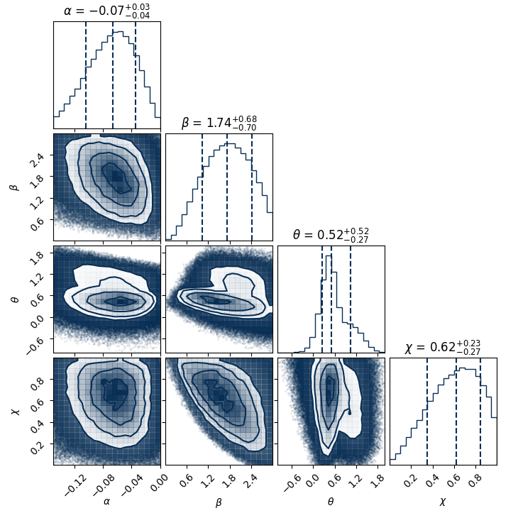
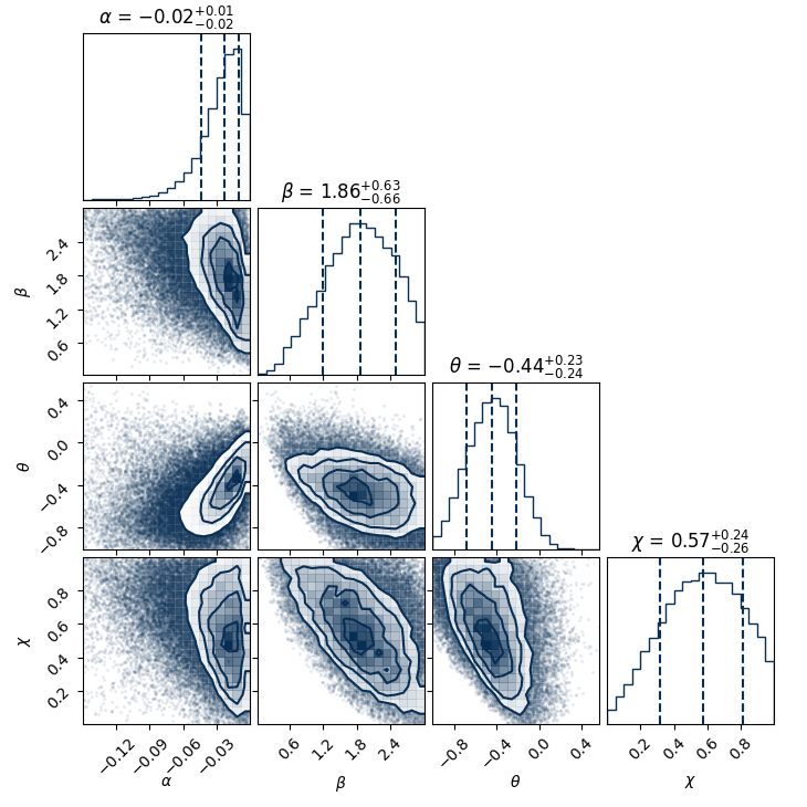
Figure 1: Corner plots showing the posterior distributions of the GTOV parameters for El3$\omega\rho$ model in the conservative scenario on the left and in the speculative scenario on the right.

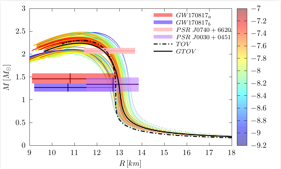
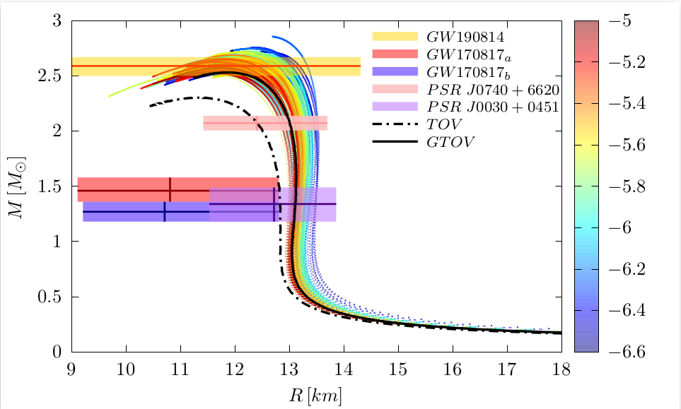
Figure 2: Mass-radius diagram for El3$\omega\rho$ model in the conservative scenario on the left and in the speculative scenario on the right.

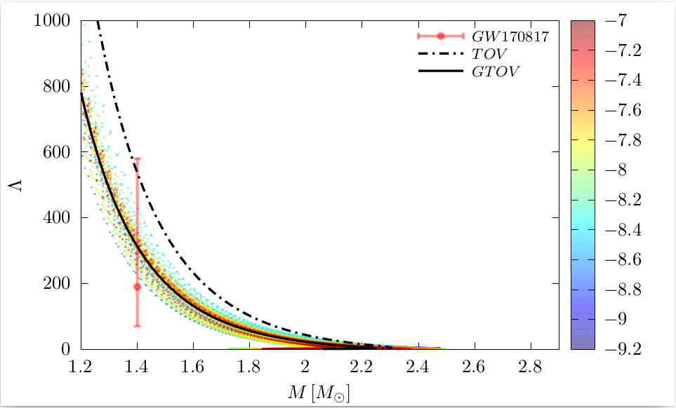
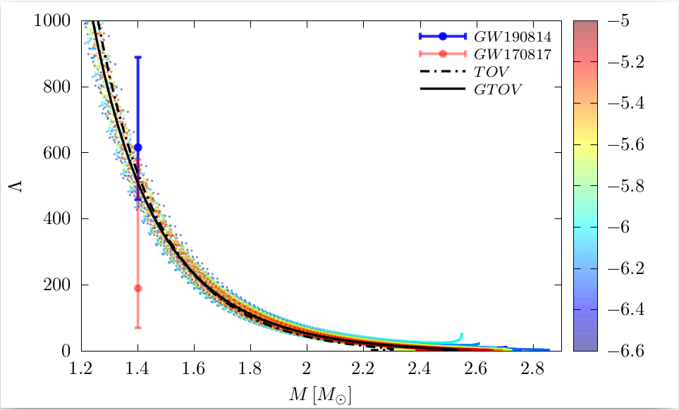
Figure 3: Tidal deformability as a function of the mass for El3$\omega\rho$ model in the conservative scenario on the left and in the speculative scenario on the right.

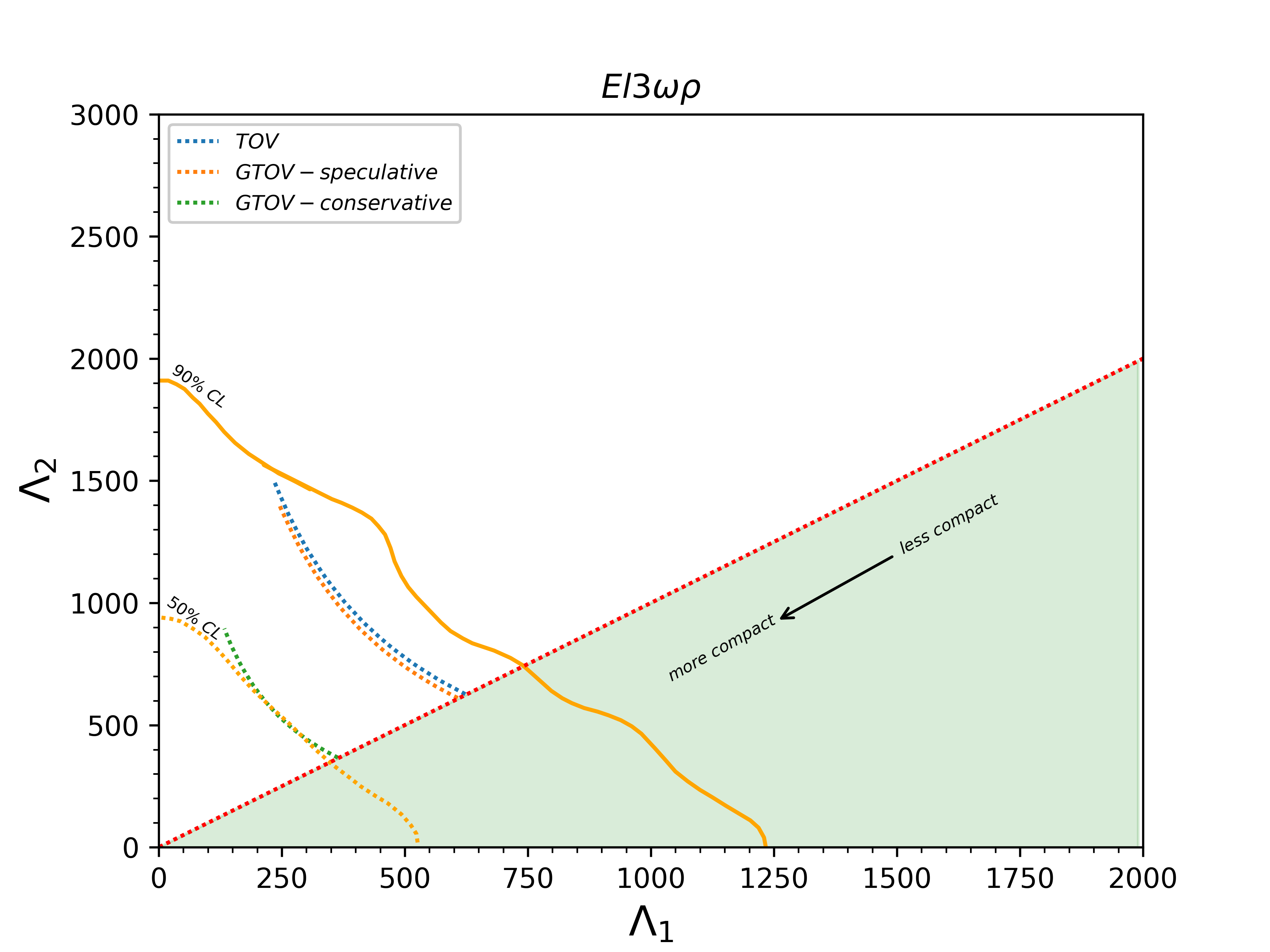
Figure 4: The dimensionless tidal deformabilities $\Lambda_{1}$ and $\Lambda_{2}$ for a binary NS system with El3$\omega\rho$ model and the same masses as in GW170817 event.

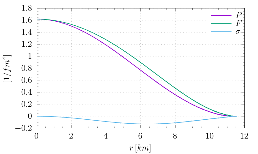
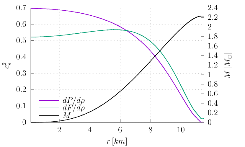
Figure 5: On the left we show the radial $P$ and transverse pressure $F$, and the anisotropy $\sigma$ as functions of the radius $r$. On the right we show the radial $(dP/d\rho)$ and transverse sound velocity $(dF/d\rho)$, and the mass $M$ as functions of the radius $r$. All plots are for a NS with central energy density $\rho_{c}=6\rho_{0}$ in the conservative scenario and for El3$\omega\rho$ model.

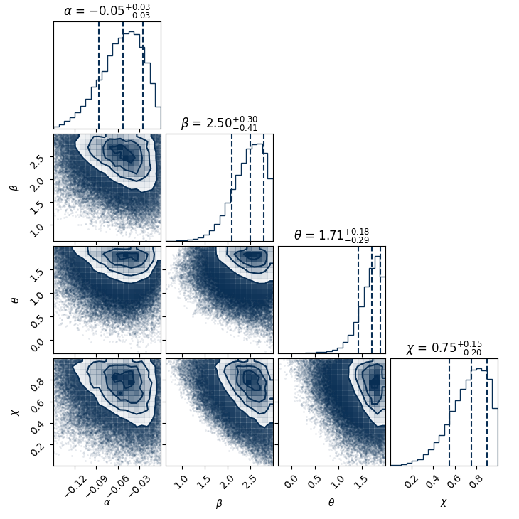
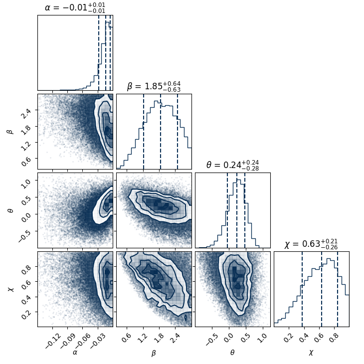
Figure 6: Corner plots showing the posterior distributions of the GTOV parameters for Nl3$\omega\rho$ model in the conservative scenario on the left and in the speculative scenario on the right.

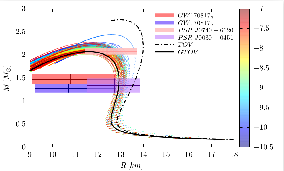
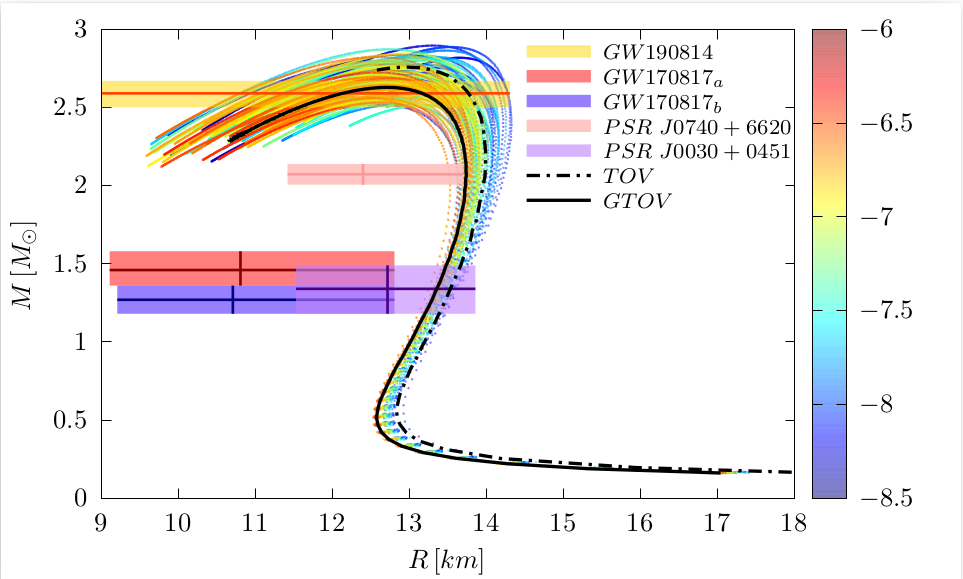
Figure 7: Mass-radius diagram for Nl3$\omega\rho$ model in the conservative scenario on the left and in the speculative scenario on the right.

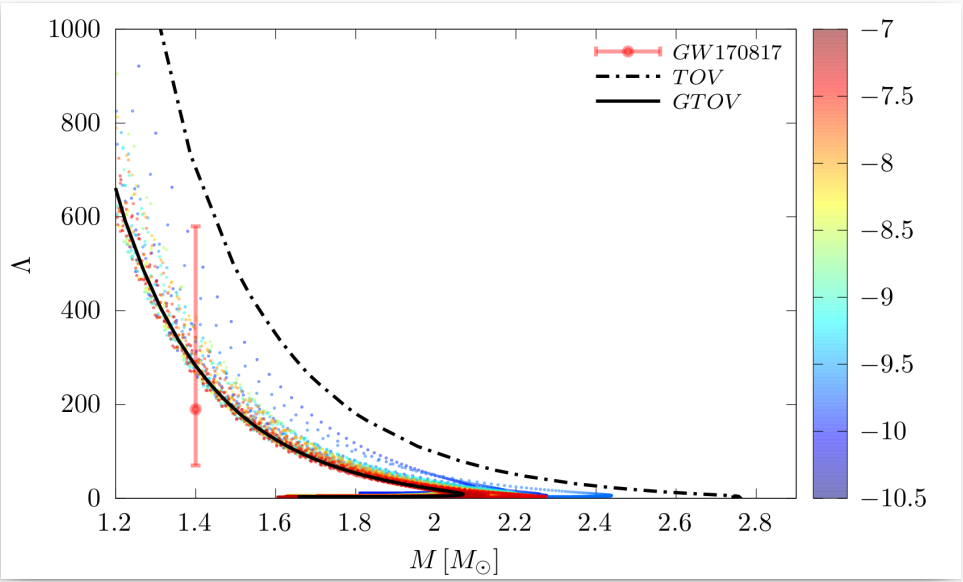
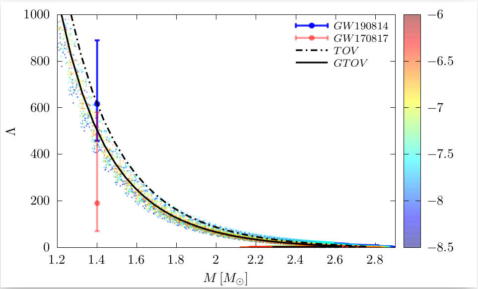
Figure 8: Tidal deformability as a function of the mass for Nl3$\omega\rho$ model in the conservative scenario on the left and in the speculative scenario on the right.

Figure 9: The dimensionless tidal deformabilities $\Lambda_{1}$ and $\Lambda_{2}$ for a binary NS system with Nl3$\omega\rho$ model and the same masses as in the GW170817 event.

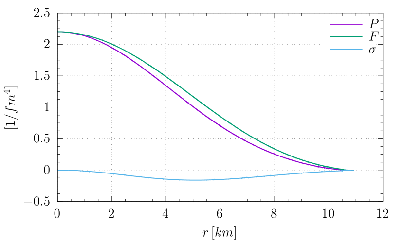
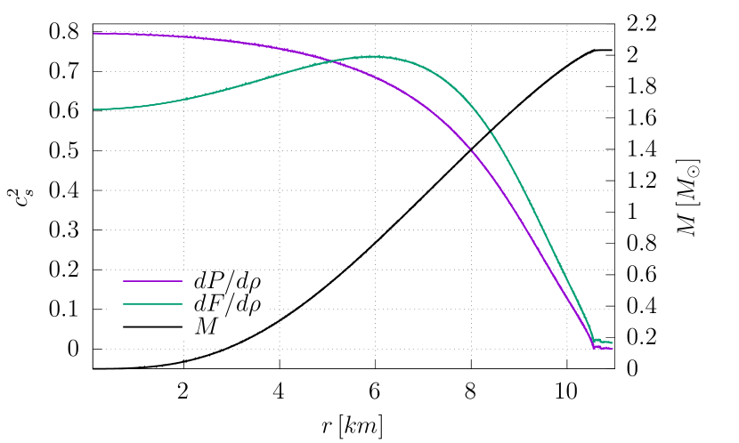
Figure 10: On the left we show the radial $P$ and transverse pressure $F$, and the anisotropy $\sigma$ as functions of the radius $r$. On the right we show the radial $(dP/d\rho)$ and transverse sound velocity $(dF/d\rho)$, and the mass $M$ as functions of the radius $r$. All plots are for a NS with central energy density $\rho_{c}=6\rho_{0}$ in the conservative scenario and for Nl3$\omega\rho$ model.

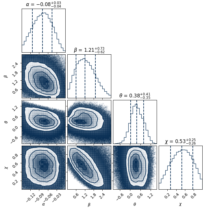
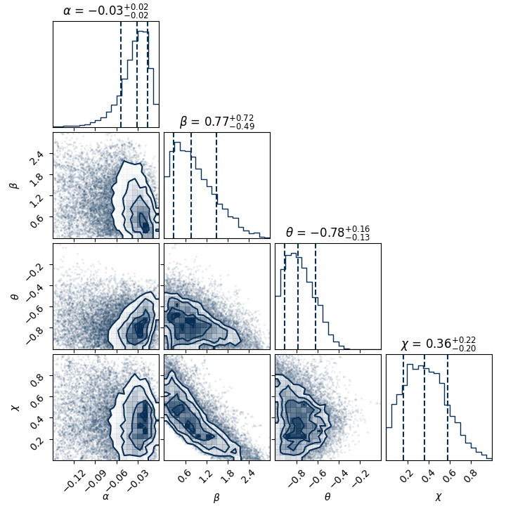
Figure 11: Corner plots showing the posterior distributions of the GTOV parameters for El3$\omega\rho$Y model in the conservative scenario on the left and in the speculative scenario on the right.

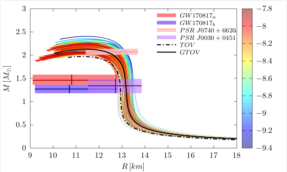
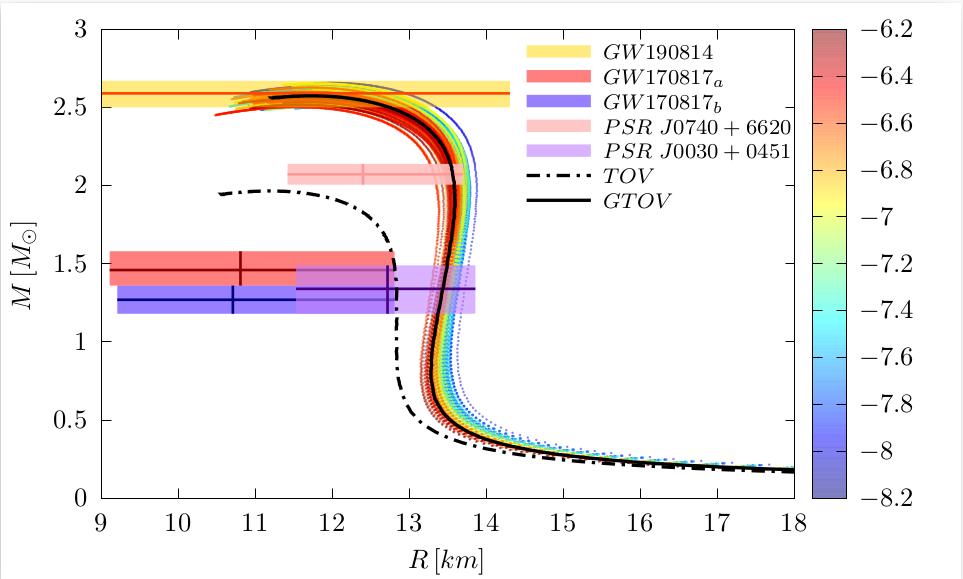
Figure 12: Mass-radius diagram for El3$\omega\rho$Y model in the conservative scenario on the left and in the speculative scenario on the right.

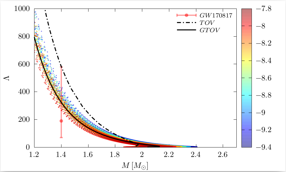
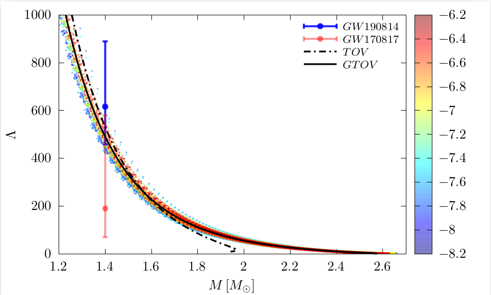
Figure 13: Tidal deformability as a function of the mass for El3$\omega\rho$Y model in the conservative scenario on the left and in the speculative scenario on the right.

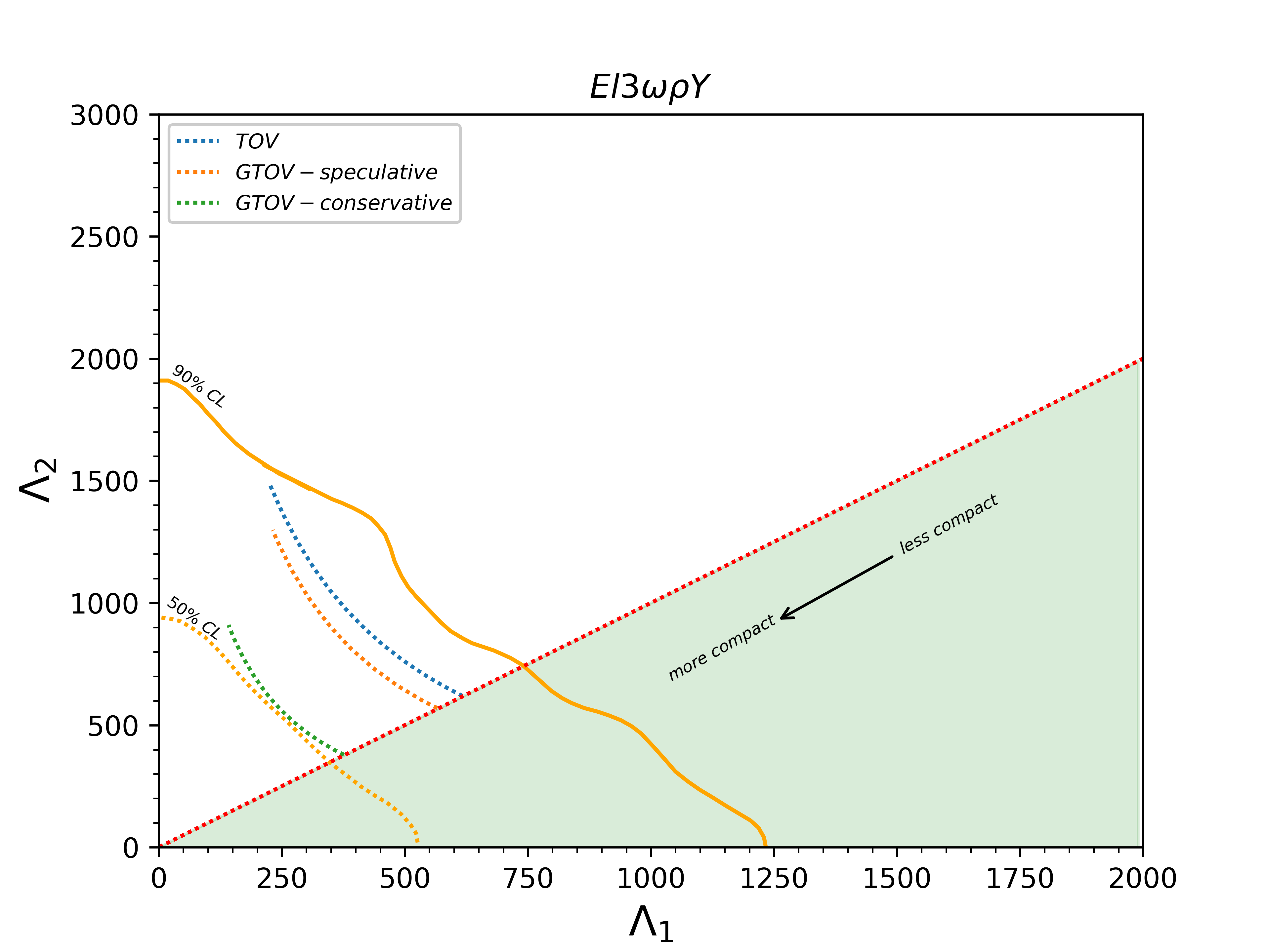
Figure 14: The dimensionless tidal deformabilities $\Lambda_{1}$ and $\Lambda_{2}$ for a binary NS system with El3$\omega\rho$Y model and the same masses as in the GW170817 event.

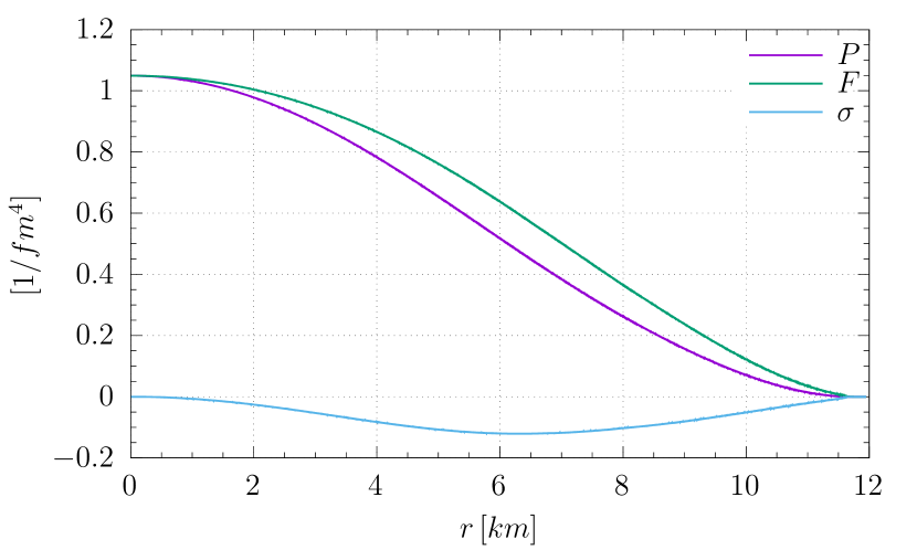
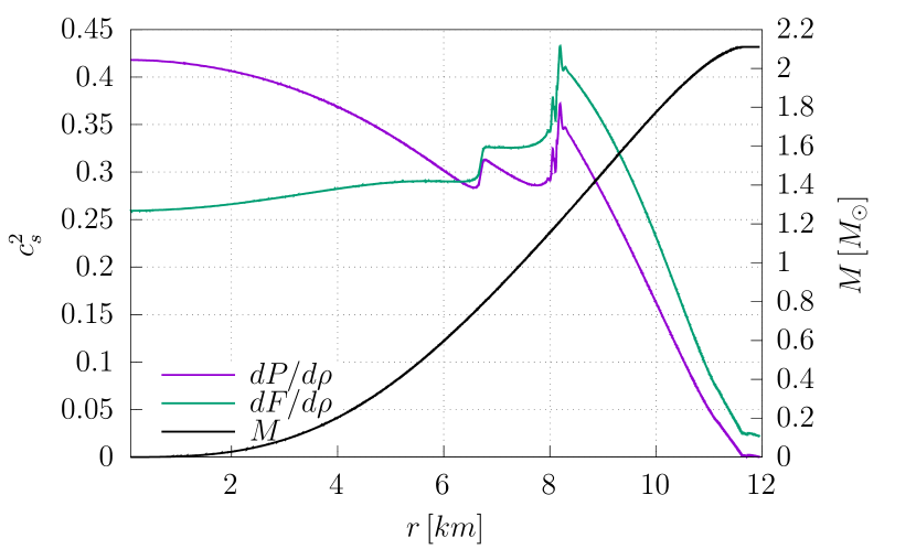
Figure 15: On the left we show the radial $P$ and transverse pressure $F$, and the anisotropy $\sigma$ as functions of the radius $r$. On the right we show the radial $(dP/d\rho)$ and transverse sound velocity $(dF/d\rho)$, and the mass $M$ as functions of the radius $r$. All plots are for a NS with central energy density $\rho_{c}=6\rho_{0}$ in the conservative scenario and for El3$\omega\rho$Y model.

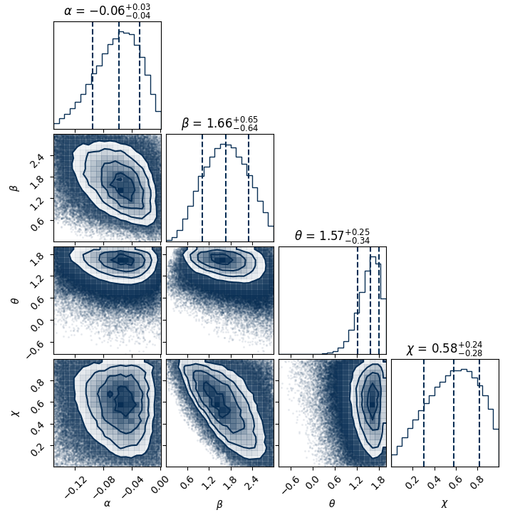
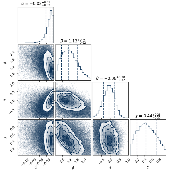
Figure 16: Corner plots showing the posterior distributions of the GTOV parameters for Nl3$\omega\rho$Y model in the conservative scenario on the left and in the speculative scenario on the right.

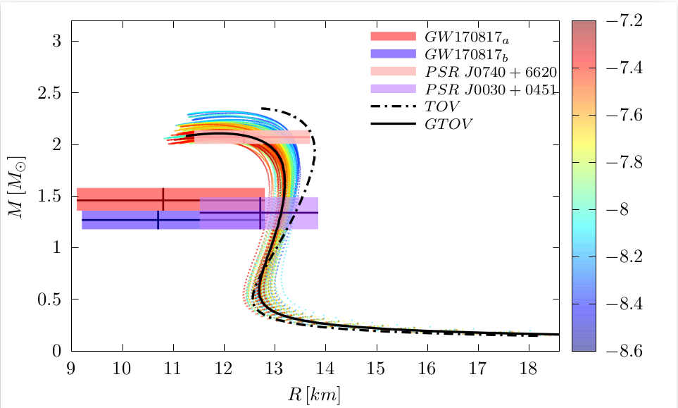
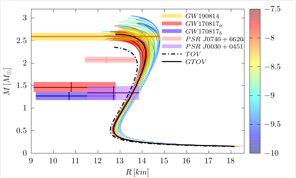
Figure 17: Mass-radius diagram for Nl3$\omega\rho$Y model in the conservative scenario on the left and in the speculative scenario on the right.

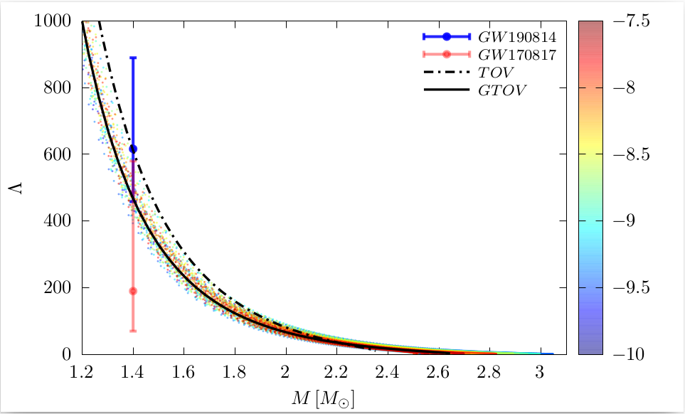
Figure 18: Tidal deformability as a function of the mass for Nl3$\omega\rho$Y model in the conservative scenario on the left and in the speculative scenario on the right.

Figure 19: The dimensionless tidal deformabilities $\Lambda_{1}$ and $\Lambda_{2}$ for a binary NS system with Nl3$\omega\rho$Y model and the same masses as in the GW170817 event.

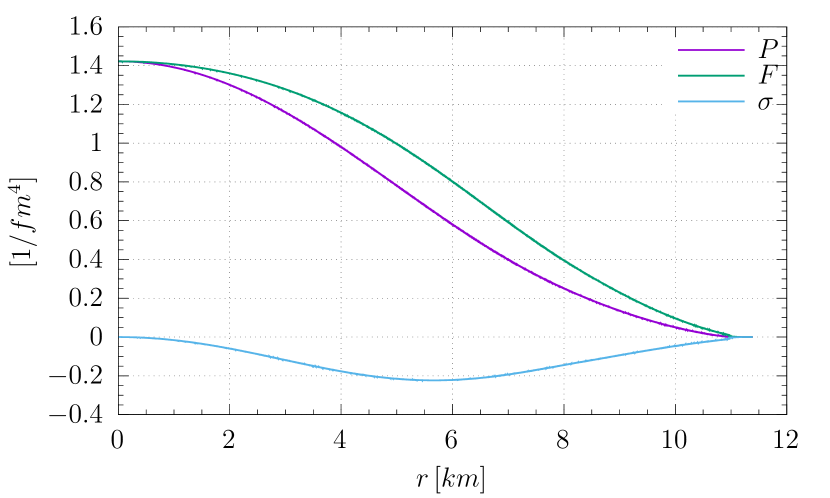
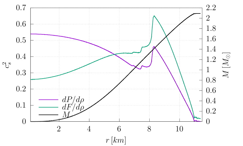
Figure 20: On the left we show the radial $P$ and transverse pressure $F$, and the anisotropy $\sigma$ as functions of the radius $r$. On the right we show the radial $(dP/d\rho)$ and transverse sound velocity $(dF/d\rho)$, and the mass $M$ as functions of the radius $r$. All plots are for a NS with central energy density $\rho_{c}=6\rho_{0}$ in the conservative scenario and for Nl3$\omega\rho$Y model.

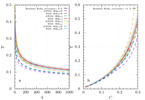
Figure 21: The dashed curves refer to GTOV solutions from each EoS parameterization, the dot-dashed curves to the TOV solution (isotropic case) also from each EoS parameterization, and the solid black line to the fit from Ref. Saes:2021fzr . These results are shown only for the conservative scenario. In the graph on the left, the only GTOV solution that approaches the error band is the one obtained from the parameterization Nl3$\omega\rho$. Meanwhile, in the graph on the right, all the GTOV solutions are within the error range for $0.05<C<0.2$, except for the parameterization El3$\omega\rho$, which diverges early.

In this section, we use Bayesian analysis to optimize the parameters $\alpha$, $\beta$, $\theta$ and $\chi$ from GTOV for the EoSs presented in Section II and assume two possible scenarios. In the first scenario, which we have called a conservative scenario, we try to optimize the GTOV parameters for the mass-radius obtained by NICER for the pulsars PSR J07740+6620 NANOGrav:2019jur and PSR J0030+0451 riley2019nicer , the mass-radius of the two NS in GW170817 event LIGOScientific:2017vwq ; LIGOScientific:2018cki ; abbott2019gwtc and the tidal deformability estimated for this event. In the second case, called speculative scenario, we consider the possibility that the compact object within the mass gap in event GW190814 LIGOScientific:2020zkf is an NS so we add its mass and tidal deformability as constraints to be fitted. In the speculative scenario, we look for values of deformability that satisfy the constraints from GW170817 and GW190814 at the same time. We assume a uniform prior for the GTOV parameters with the domain of the parameters being taken from the Rahmansyah A., et al. paper gtovprd , so that we have: $\alpha\in[-0.15,0.15]$, $\beta\in[0,3]$, $\theta\in[-1,2]$ and $\chi\in[0,1]$. As in da2024bayesian , we assume a Gaussian likelihood function and set causal limits for the mass (M${}_{max}<3.2$ M_⊙) rhoades1974maximum and, for the radius ($R>3GM/c^{2}$), and our posterior distributions are obtained using the emcee package foreman2013emcee . The package uses the method of Goodman and Weare’s Affine Invariant Markov Chain Monte Carlo (MCMC) Goodman for sampling the posterior probability density.

In Figs. 1, 6, 11 and 16, we show the corner plots corner of the posterior distributions for the GTOV parameters ($\alpha$, $\beta$, $\theta$, $\chi$) when we assume that matter inside the neutron stars can be described by the El3$\omega\rho$, Nl3$\omega\rho$, El3$\omega\rho$Y and Nl3$\omega\rho$Y EoSs, respectively. The dashed vertical lines in the 1D histograms represent the 0.16, 0.5, and 0.84 quartiles of each histogram. The contour levels in the 2D histograms represent the 0.5, 1, 1.5 and 2$\sigma$ levels containing $11.8\%$, $39.3\%$, $67.5\%$ and $86.4\%$ of the samples for each case, respectively corner .

In Figs. 2, 7, 12 and 17, we show the mass-radius diagrams for the El3$\omega\rho$, Nl3$\omega\rho$, El3$\omega\rho$Y and Nl3$\omega\rho$Y EoSs, respectively. The black dash-dotted curves are the mass-radius for TOV and the black continuous curves are the mass-radius for GTOV using the central values of the parameters obtained in the Bayesian inferences. The colorful dotted curves are the mass-radius curves obtained using values for the GTOV parameters that are within the $68\%$ Credible Interval (CI) of the log posterior distributions, considering the Highest Density Interval (HDI). The color palette to the right of the plots shows the correspondence between the color of each curve and its log posterior value. These figures also show masses and radii used as constraints in the Bayesian inferences: the two NS in the GW170817 event LIGOScientific:2017vwq ; LIGOScientific:2018cki ; abbott2019gwtc , one of them with a mass M${}_{1}=1.46^{+0.12}_{-0.10}$ M_⊙ (dark pink continuous horizontal line) and radius R${}_{1}=10.8^{+2.0}_{-1.7}$ km (dark pink continuous vertical line) and the other one with a mass of M${}_{2}=1.27^{+0.09}_{-0.09}$ M_⊙ (dark purple continuous horizontal line) and radius R${}_{2}=10.7^{+2.1}_{-1.5}$ km (dark purple continuous vertical line); and the two stars from NICER, PSR J07740+6620 NANOGrav:2019jur with a mass $2.072^{+0.067}_{-0.066}$ M_⊙ (light pink continuous horizontal line) and radius $12.39^{+1.30}_{-0.98}$ km (light pink continuous vertical line) and PSR J0030+0451 riley2019nicer with mass $1.34^{+0.15}_{-0.16}$ M_⊙ (light purple continuous horizontal line) and radius $12.71^{+1.14}_{-1.19}$ km (light purple continuous vertical line); with the shaded regions indicating the uncertainty in the estimated values. The figures for the speculative case also display the mass ($2.5^{+0.08}_{-0.09}$ M_⊙) of the possible NS in the event GW190814 LIGOScientific:2020zkf as an orange continuous horizontal line and a shaded region for its the uncertainty.

In Figs. 3, 8, 13 and 18 we show the dimensionless tidal deformability $\Lambda$ as a function of the mass M [M_⊙] for the El3$\omega\rho$, Nl3$\omega\rho$, El3$\omega\rho$Y and Nl3$\omega\rho$Y EoSs, respectively. Similarly to the mass-radius diagrams, the black dash-dotted curves represent the GR case and the black continuous curves correspond to the $\Lambda\times$ M [M_⊙] curves using the central values of the GTOV parameters found in the Bayesian inferences. Here too, the colorful dotted curves are the ones obtained using values from the GTOV parameters that are within the $68\%$ CI of the log posterior distributions. The value of $\Lambda_{1.4}$ estimated for the GW170817 event, $\Lambda_{1.4}=190^{+390}_{-120}$ at 90% confidence level LIGOScientific:2017vwq , is shown as a red dot with its corresponding error bar. In the speculative case, we also show the value of $\Lambda_{1.4}$ estimated for the GW190814 event, $\Lambda_{1.4}=616^{+273}_{-158}$ LIGOScientific:2020zkf , represented by a blue dot with an error bar.

In the left panel of Figs. 4, 9, 14 and 19 we show the dimensionless tidal deformabilities $\Lambda_{1}$ and $\Lambda_{2}$ obtained for a binary NS system that has the same chirp mass of the GW170817 event, $\mathcal{M}=1.188~{}\text{M}_{\odot}$. This way, the masses $m_{1}$ and $m_{2}$ of the two NS in the system are related in the following way

$$\mathcal{M}=\frac{(m_{1}m_{2})^{3/5}}{(m_{1}+m_{2})^{1/5}},$$ (31)

where the values of $m_{1}$ and $m_{2}$ are in the same range of values as masses of the NS in GW170817, i.e., $1.36\leq m_{1}[\text{M}_{\odot}]\leq 1.58$ and $1.18\leq m_{2}[\text{M}_{\odot}]\leq 1.36$. We have calculated $\Lambda_{1}$ and $\Lambda_{2}$ for each EoS in GR (blue dotted curve) and in the conservative (green dotted curve) and speculative (orange dotted curve) scenarios using the central values of the GTOV parameters obtained in each inference and using the El3$\omega\rho$, Nl3$\omega\rho$, El3$\omega\rho$Y and Nl3$\omega\rho$Y EoSs. The diagonal red dotted line designates the boundary $\Lambda_{1}=\Lambda_{2}$. We also show the $50\%$ credible levels (orange dotted curve) and $90\%$ CL (orange continuous curve) determined by LIGO/Virgo in the low-spin prior scenario LIGOScientific:2017vwq for the posteriors obtained using EOS-insensitive relations.

On the right plot of Figs. 5, 10, 15 and 20, the first one shows both radial pressure and transverse pressure against the radius of one star for $\rho=6\rho_{0}$ and $\sigma$, where $\sigma$ shows the behavior between P and F. In the second plot, the transverse and radial speed of sound squared against radius is shown. The neutron star mass against radius is also presented. The radial speed of sound against $r$, shows the appearance of hyperons through abrupt modifications in its pattern. The hyperons that appear for each drop - for these parameterizations - in the speed of sound squared are $\Lambda$, $\Sigma^{-}$ and $\Xi^{-}$ (absent only in the plot), respectively. As a requirement for an anisotropic star, we can see - except for $\rho>0$ and $\frac{d\rho}{dr}<0$, which is not shown - that all conditions in III.1 are satisfied.

From the El3$\omega\rho$ EoS, we observed that the GTOV parameters $\alpha$, $\theta$, and $\chi$ show a significant deviation from the GR case in the conservative case than the speculative one as shown in Fig. 1. Particularly, we determined $\theta>0$ in the conservative case and $\theta<0$ in the speculative picture. Moreover, the GR model produces a mass-radius diagram that satisfies the NICER and the GW170817 data with $\Lambda_{1.4}$ falling within the upper margin of error of the value determined for the binary system that participated in the GW170817 event, as shown in Figs. 2 and 3 respectively. On the other hand, the GTOV curves in both the conservative and the speculative scenarios have relatively higher radii, but the conservative case satisfies NICER and the GW170817 data as shown on the same graphs. However, the value of $\Lambda_{1.4}$ falls within the central limit in the conservative case, and in the speculative case the value for $\Lambda_{1.4}$ determined for both GTOV and GR curves fall within the lower error margin of the GW190814 event aside satisfying GW170817 event at the upper limit. Generally, the GTOV case produces stars with higher $\rm M_{max}$ and enhanced compactness in the speculative scenario compared to the GR case. In the conservative case, $\rm M_{max}$ is reduced and the compactness is higher than in both GR and speculative scenario.

In the case of Nl3$\omega\rho$ EoS, we observe a major deviation of the GTOV parameters in the conservative case from the one obtained from GR. Under this analysis, we found $\theta>0$ in conservative and speculative cases as shown in Fig. 6. With this EoS, we obtain a massive star with $\rm M_{max}=2.74M_{\odot}$ in GR as shown in Fig. 7, satisfying the PSR J0030+0451 mass-radius data. This lead to $\Lambda_{1.4}$ that strongly satisfies GW190814 and violates GW170817 as presented in Fig. 8. On the other hand, the GTOV curve in the speculative case satisfies the mass-radius data for GW190814 and NICER, while in the conservative case, it slightly violates the GW170817 data with comparatively smaller $\rm M_{max}$. This produces a $\Lambda_{1.4}$ that strongly satisfies GW170817 in the conservative picture, and in the speculative picture, GW170817 and GW190814 are satisfied by GR and GTOV parameterizations as shown in Fig. 8 (right). In contrast, in the speculative case where higher $\rm M_{max}$ are expected, the deviation of the mass-radius curves for both GR and GTOV is smaller as compared to the conservative cases. Based on the afore analysis and Fig. 9, we can infer that the conservative analysis of GTOV using Nl3$\omega\rho$ yields more compact stars than El3$\omega\rho$, below the 50% CI (note that the lesser the percentage the more compact the star). The same is true with the speculative case where the curve is between the 90% CI. Generally, the GR model produces less compact NSs than the GTOV as the figures show.

Employing the El3$\omega\rho$Y EoS, which is the addition of hyperons to El3$\omega\rho$ EoS, we highlight the behavior of GTOV parameters under different scenarios relative to the GR model. The conservative scenario shows significant deviation in the GTOV parameters $\alpha$, $\beta$, and $\chi$ than the speculative scenario, with $\theta>0$ in the conservative case and $\theta<0$ in the speculative case as shown in Fig. 11. The addition of hyperons to the El3$\omega\rho$ model reduces the maximum mass achievable from GR, failing to satisfy the mass constraint of PSR J0740+6620 and GW170817. However, the GTOV equations satisfy the mass-radius constraint of the NICER pulsars with slightly higher radii (the upper region of the error bar) that do not satisfy the GW data as presented in Fig. 12. The tidal deformability parameter $\Lambda_{1.4}$ increases with hyperons, shifting the $\Lambda_{1.4}$ toward the upper limit of the value determined in the GW170817 event, in the conservative scenario. On the other hand, the $\Lambda_{1.4}$ shifts closer to the lower limit of GW190814 value, in the speculative case, as shown in Fig. 13 (right). In the speculative case, the $\Lambda_{1.4}$ satisfies the GW190814 and GW170817 data and the mass achieves the $\rm M_{max}$ required, see Figs. 13 and 12 (right). The mass-radius diagram shows significant differences between GR and GTOV in both the conservative and the speculative scenarios, with the latter resulting in more compact NSs compared to the former, as shown in Fig. 14. It is worth mentioning that the stars produced in the speculative scenario using El3$\omega\rho$Y EoS are more compact than the ones built from El3$\omega\rho$.

Using the Nl3$\omega\rho$Y EoS which is a hyperonized version of Nl3$\omega\rho$ EoS, we determined the GTOV parameters relative to the GR case once more. We consider conservative and speculative cases in the analysis. The speculative analysis shows a significant deviation of the GTOV parameters from the GR one, with $\theta>0$ in the conservative case and $\theta<0$ in the speculative case as shown in Fig. 16. We find that hyperonization of the EoS leads to a reduction in the $\rm M_{max}$ with relatively higher radii which satisfies PSR J0030+0451 in the GR case. The GTOV equations, on the other hand, produce a mass-radius relation that is in good agreement with the observed NICER pulsars used in the conservative analyses, however, it fails to satisfy the GW170817 data as displayed in Fig. 17. Also, in the speculative case, the GTOV equations show a good agreement with the GW190814 data with significantly larger radii, failing to satisfy the GW170817 data for $\Lambda_{1.4}$. Additionally, the hyperonized EoS considered here produces smaller $\Lambda_{1.4}$ in general. However, the GR model mildly satisfies the GW170817 data at its uppermost error limit, on the contrary, the GTOV equations agree well with the GW170817 data in the conservative analysis as shown in Fig. 18. In the speculative case, the GR and GTOV parameterizations satisfy both GW170817 and GW190814 data. In Fig. 19, we observe that the presence of hyperons shows no significant effect on the $\Lambda_{1}-\Lambda_{2}$ diagram in the conservative case. In contrast, stars composed of hyperons are found to be more compact.

The only parameters related to observational constraints are $\alpha$ and $\chi$ Narimani:2014zha ; Rappaport:2007ct . The authors of Ref. Narimani:2014zha extracted $0.04\lesssim\alpha\lesssim 0.15$ from the observations. The parameter $\chi$ was obtained by fitting the big bang nucleosynthesis (BBN), having the following values: $\chi=1.0\pm 0.14$ and $\chi=0.84\pm 0.25$. There are two values of $\chi$ because two values of primordial helium mass fraction ($Y_{p}$) were used Rappaport:2007ct . The fitting of this parameter does not depend strongly on the observational details involved. From conditions (3), (4), and (5) mentioned in III.1 near the center of the star $(\sigma_{c}\rightarrow 0)$, the authors of Ref. gtovprd showed that $1/3\leq\Upsilon_{c}\leq 1$, where $\Upsilon_{c}=P_{c}/\rho_{c}$. The minimum value of $\Upsilon_{c}$ is compatible with that obtained by Saes:2021fzr which is $\Upsilon_{min}\approx 0.3$. Universal relations — insensitive kent1 ; kent2 to the EoS — have proven useful for extracting properties of nuclear matter, as they connect macroscopic and microscopic properties of the NS. One way to break the degeneracies in data analysis and model selection for different observations such as radio, X-ray, and gravitational waves is by using universal relationsYagi:2015hda . The authors of Ref. Yagi:2015hda found that the I-Love-Q relations are still valid up to 10 $\%$ of the isotropic case. In this work, they used two simple models for pressure anisotropy. In other words, it will depend on the value of the anisotropy used and the model. In our work, this value is associated with the GTOV parameters. Ref. Saes:2021fzr found for GR an approximate universal relation between $\Upsilon-C/\Lambda/\bar{I}$ for 25 realistic EoSs. The $\Upsilon$ can be viewed as a mean notion of the stiffness of nuclear matter inside the NS. The tolerance of universal relations varies for each pair. Therefore, the maximum error is different for each graph below. The same occurs in Yagi:2015hda for I-Love-Q relations.

In Fig. 21, one can note that $\Upsilon-C/\Lambda$ relations are maintained for isotropic case GR. Meanwhile, for the case of anisotropic case (GTOV), only $\Upsilon-C$ are within the error band for certain EoSs and GTOV parameters. It is worth mentioning that for other values of $\alpha$, $\beta$, $\theta$, and $\chi$, it would be possible to be within the error band provided by Ref. Saes:2021fzr , i.e., for a weaker anisotropy.

EoS	Scenario	$(\alpha,\beta,\theta,\chi)$	$M_{max}$ $[M_{\odot}]$	$R_{max}$ [km]	$\Lambda_{1.4}$	$R_{1.4}$ [km]
El3$\omega\rho$Y	speculative	(-0.03, 0.77,-0.78, 0.36)	2.57 ✓	11.72	490 ✓ ✓	13.44 ✓ ✓
El3$\omega\rho$	speculative	(-0.02, 1.85, -0.44, 0.57)	2.53 ✓	11.87	509 ✓ ✓	13.10 ✓ ✓
Nl3$\omega\rho$Y	speculative	(-0.02, 1.13, -0.08, 0.44)	2.63 ✓	13.18	467 ✓ ✓	13.62 ✓ ✓
Nl3$\omega\rho$	speculative	(-0.01, 1.85, 0.24, 0.63)	2.62 ✓	12.49	504 ✓ ✓	13.40 ✓ ✓
El3$\omega\rho$Y	conservative	(-0.08, 1.21, 0.38, 0.53)	2.12 ✓	11.37 ✓	323 ✓	13.14 ✓ ✓
El3$\omega\rho$	conservative	(-0.07, 1.74, 0.52, 0.62)	2.24 ✓	11.31 ✓	312 ✓	12.94 ✓ ✓
Nl3$\omega\rho$Y	conservative	(-0.06, 1.66, 1.57, 0.58)	2.19 ✓	11.74 ✓	287 ✓	13.13 ✓✓
Nl3$\omega\rho$	conservative	(-0.05, 2.5, 1.71, 0.75)	2.06 ✓	11.71 ✓	282 ✓	12.91 ✓ ✓
El3$\omega\rho$Y	GR	(0, 1, 0, 1)	1.96	11.43	530 ✓ ✓	12.81 ✓ ✓
El3$\omega\rho$	GR	(0, 1, 0, 1)	2.30 ✓	11.22 ✓	536 ✓ ✓	12.81 ✓ ✓
Nl3$\omega\rho$Y	GR	(0, 1, 0, 1)	2.35 ✓	12.73 ✓	611 ✓	13.45 ✓ ✓
Nl3$\omega\rho$	GR	(0, 1, 0, 1)	2.74 ✓	12.64	619 ✓	13.45 ✓ ✓

Table 2: Here, we make a comparison between our results and the values used in the Bayesian analysis. For the dimensionless tidal deformability, we use $\Lambda_{1.4}(GW170817)=190^{+390}_{-120}$ and $\Lambda_{1.4}(GW190814)=616^{+273}_{-158}$. While for masses and radii, we have: mass (GW190814) = $2.5^{+0.08}_{-0.09}$ M_⊙, mass(PSR J07740+6620) = $2.072^{+0.067}_{-0.066}$ M_⊙ and radius $12.39^{+1.30}_{-0.98}$ km, mass (PSR J0030+0451) = $1.34^{+0.15}_{-0.16}$ M_⊙ and radius $12.71^{+1.14}_{-1.19}$ km

.

V Conclusions

In this work, we use Bayesian inference to optimize the GTOV parameters to satisfy recent astrophysical data from NICER and GW detections, considering four EoS parameterizations. We set our prior distributions based on the values for the GTOV parameters obtained in gtovprd . Unlike in their work, we do not define each parameter set according to a physical condition such as $\sigma=0$ at the center of the star, but rather use the minimum and maximum values of each parameter suggested by them. Using the available observational data about mass, radius, and dimensionless tidal deformability for the likelihood distribution, we find the condition $\sigma=0$ at the center of the star, as can be seen in Figs. 5, 10, 15 and 20 on the right. However, using their expression for $\sigma$, we obtained a negative alpha. Moreover, if we analyze only the mass-radius diagram without calculating the dimensionless tidal deformability in our code, the alpha can be positive in agreement with clesio ; gtovprd . However, when including the dimensionless tidal deformability, the code runs only for negative alpha. This is mainly because when computing the dimensionless tidal deformability the value of the denominator $(1-d\sigma/dP)$ tends to zero for $\alpha>0$, leading to unphysical solutions. In velten2016 , negative values of $\alpha$ were also tested, and the authors concluded that values of alpha smaller than zero lead to an increase in the mass and the radius. We must point out that in their work, the dimensionless tidal deformability was not calculated. In our work, however, we found that when we combine the variation of the other three parameters ($\beta,~{}\theta$ and $\chi$) simultaneously it is possible to have $\alpha<0$ and an increase on both the mass and the radius, see Fig. 7 for example.

We used two possible constraint scenarios - conservative and speculative - and four different EoS parameterizations to constrain the GTOV parameters. In the conservative scenario, we used mass-radius data from NICER and the GW170817 event plus the data for the tidal deformability from the GW170817, and in the speculative scenario, we also considered the possibility that the compact object that falls within the mass gap in the GW190814 event is a NS, so its mass and deformability were added to the constraints. In Table 2, one can notice how the GTOV parameters changed M, R, and $\Lambda$ to be close to the observational data. We can observe that with GTOV we were able to satisfy the constraints of tidal deformability coming from the GW events in all cases considered. However, in the mass-radius diagram and tidal deformability, we see that none of these results satisfied all the imposed constraints at the same time. Another interesting aspect is that using GTOV both parameterizations, with and without hyperons, lead to similar values for M, R, and $\Lambda$. Besides, we emphasize that, without the parameterization of the $\Phi$ field related to EoS with hyperons (if $\alpha<1$, this cause an increase in mass-radius relation, here we used $\alpha=1$) the degree of anisotropy from GTOV would be higher, since it would be necessary to increase the pressure to achieve a NS with a mass $\sim$ $2M_{\odot}$

On the other hand, when we disregard the masses and radii of $M_{1}$ and $M_{2}$ from GW170817, we see that both the TOV and the GTOV present better results in both the conservative and the speculative scenario. In the conservative scenario, all results approach the central value of the tidal deformability from GW170817. Three of our results are within the expected $\chi$ value set by Rappaport:2007ct : Nl3$\omega\rho$ in both the conservative and the speculative scenario and El3$\omega\rho$ in the conservative scenario. As for the alpha values, we cannot make a direct comparison with previous results, since our results have a different $\alpha$-sign.

Additionally, we analyzed the approximate universal relations of $\Upsilon-C/\Lambda$. In GR, all the parameterizations used here respected the error margin. However, for GTOV the relation $\Upsilon-C/\Lambda$ gives a good result only for Nl3$\omega\rho$ in the conservative scenario, since the values of $\Lambda<200$ and $C<0.25$ of these relations are satisfied. Some works have recalculated these universal relations for anisotropic stars with realistic EoS Biswas:2019gkw ; Das:2022ell . However, assuming that the results from modified theories of gravity should not diverge significantly from those of GR, the same applies here. In other words, the universal relations obtained for isotropic stars using realistic EoSs are essential for determining the error margin in our results for GTOV. It is worth noticing that in the GTOV context, the anisotropy arises from modified theories of gravity and not from an anisotropy model Bowers ; Horvat_2011 ; Cosenza:1981myi .

We conclude that the conservative scenario with the Nl3$\omega\rho$ EoS is the most plausible based on our analysis. Since the value of $\alpha$ is small, $\chi$ approaches the expected value Rappaport:2007ct . However, $\beta$ and $\theta$ deviate significantly from the GR values. In other words, anisotropy associated to the GTOV parameters is necessary primarily to obtain a value of $\Lambda_{1.4}$ close to the central value used in the Bayesian analysis. Additionally, the different EoS parameterizations could lead to different values for the GTOV parameters. If we combine the results that are inside the $68\%$ CI of the four EoS models in the conservative scenario we obtain that the best estimate for the value of the GTOV parameters is $\alpha=-0.07^{+0.03}_{-0.04}$, $\beta=1.71^{+0.74}_{-0.74}$, $\theta=0.65^{+0.93}_{-0.41}$ and $\chi=0.61^{+0.23}_{-0.28}$. Finally, an observational challenge is to distinguish the origin of the anisotropy and its effects on neutron star characteristics, as these effects can be caused by a softer or stiffer EoS. There are many proposals for the origin of the anisotropy (for a review, see Herrera:1997plx ), such as very high magnetic field, phase transitions, pion condensation, crystallization of the core, relativistic nuclear interaction, and superfluid core.

References

- (1) K. C. Gendreau et al., “The Neutron star Interior Composition Explorer (NICER): design and development,” in Space Telescopes and Instrumentation 2016: Ultraviolet to Gamma Ray (J.-W. A. den Herder, T. Takahashi, and M. Bautz, eds.), vol. 9905, p. 99051H, International Society for Optics and Photonics, SPIE, 2016.
- (2) S. Typel et al., “CompOSE Reference Manual,” The European Physical Journal A, vol. 58, no. 11, p. 221, 2022.
- (3) T. E. Riley, A. L. Watts, S. Bogdanov, P. S. Ray, R. M. Ludlam, S. Guillot, Z. Arzoumanian, C. L. Baker, A. V. Bilous, D. Chakrabarty, et al., “A NICER view of PSR J0030+0451: Millisecond pulsar parameter estimation,” The Astrophysical Journal Letters, vol. 887, no. 1, p. L21, 2019.
- (4) T. E. Riley, A. L. Watts, P. S. Ray, S. Bogdanov, S. Guillot, S. M. Morsink, A. V. Bilous, Z. Arzoumanian, D. Choudhury, J. S. Deneva, et al., “A NICER view of the massive pulsar PSR J0740+ 6620 informed by radio timing and XMM-Newton spectroscopy,” The Astrophysical Journal Letters, vol. 918, no. 2, p. L27, 2021.
- (5) G. Raaijmakers, T. E. Riley, A. L. Watts, S. K. Greif, S. M. Morsink, K. Hebeler, A. Schwenk, T. Hinderer, S. Nissanke, S. Guillot, et al., “A NICER view of PSR J0030+ 0451: Implications for the dense matter equation of state,” The Astrophysical Journal Letters, vol. 887, no. 1, p. L22, 2019.
- (6) S. Bogdanov, S. Guillot, P. S. Ray, M. T. Wolff, D. Chakrabarty, W. C. G. Ho, M. Kerr, F. K. Lamb, A. Lommen, R. M. Ludlam, et al., “Constraining the neutron star mass–radius relation and dense matter equation of state with NICER. i. the millisecond pulsar x-ray data set,” The Astrophysical Journal Letters, vol. 887, no. 1, p. L25, 2019.
- (7) M. C. Miller, F. K. Lamb, A. J. Dittmann, S. Bogdanov, Z. Arzoumanian, K. C. Gendreau, S. Guillot, A. K. Harding, W. C. G. Ho, J. M. Lattimer, et al., “PSR J0030+0451 mass and radius from NICER data and implications for the properties of neutron star matter,” The Astrophysical Journal Letters, vol. 887, no. 1, p. L24, 2019.
- (8) B. P. Abbott et al., “GW170817: Observation of Gravitational Waves from a Binary Neutron Star Inspiral,” Physical Review Letters, vol. 119, no. 16, p. 161101, 2017.
- (9) B. P. Abbott, R. Abbott, T. Abbott, F. Acernese, K. Ackley, C. Adams, T. Adams, P. Addesso, R. Adhikari, V. Adya, et al., “Gravitational waves and gamma-rays from a binary neutron star merger: Gw170817 and grb 170817a,” The Astrophysical Journal Letters, vol. 848, no. 2, p. L13, 2017.
- (10) B. P. Abbott, R. Abbott, T. D. Abbott, F. Acernese, K. Ackley, C. Adams, T. Adams, P. Addesso, R. X. Adhikari, V. B. Adya, et al., “Multi-messenger observations of a binary neutron star merger,” The Astrophysical Journal Letters, vol. 848, p. L12, oct 2017.
- (11) B. P. Abbott et al., “GW170817: Measurements of neutron star radii and equation of state,” Physical Review Letters, vol. 121, no. 16, p. 161101, 2018.
- (12) O. Lourenço, M. Dutra, C. H. Lenzi, C. V. Flores, and D. P. Menezes, “Consistent relativistic mean-field models constrained by GW170817,” Physical Review C, vol. 99, no. 4, p. 045202, 2019.
- (13) O. Lourenço, M. Dutra, C. H. Lenzi, S. K. Biswal, M. Bhuyan, and D. P. Menezes, “Consistent Skyrme parametrizations constrained by GW170817,” The European Physical Journal A, vol. 56, no. 2, p. 32, 2020.
- (14) L. L. Lopes, “Hyperonic neutron stars: reconciliation between nuclear properties and NICER and LIGO/VIRGO results,” Communications in Theoretical Physics, vol. 74, no. 1, p. 015302, 2021.
- (15) G. Raaijmakers, S. K. Greif, T. E. Riley, T. Hinderer, K. Hebeler, A. Schwenk, A. L. Watts, S. Nissanke, S. Guillot, J. M. Lattimer, et al., “Constraining the dense matter equation of state with joint analysis of NICER and LIGO/Virgo measurements,” The Astrophysical Journal Letters, vol. 893, no. 1, p. L21, 2020.
- (16) G. Raaijmakers, S. K. Greif, K. Hebeler, T. Hinderer, a. Nissanke, A. Schwenk, T. E. Riley, A. L. Watts, J. M. Lattimer, and W. C. G. Ho, “Constraints on the dense matter equation of state and neutron star properties from NICER’s mass–radius estimate of PSR J0740+ 6620 and multimessenger observations,” The Astrophysical Journal Letters, vol. 918, no. 2, p. L29, 2021.
- (17) D. Radice, A. Perego, F. Zappa, and S. Bernuzzi, “GW170817: joint constraint on the neutron star equation of state from multimessenger observations,” The Astrophysical Journal Letters, vol. 852, no. 2, p. L29, 2018.
- (18) T. Malik, N. Alam, M. Fortin, C. Providência, B. K. Agrawal, T. K. Jha, B. Kumar, and S. K. Patra, “GW170817: Constraining the nuclear matter equation of state from the neutron star tidal deformability,” Physical Review C, vol. 98, no. 3, p. 035804, 2018.
- (19) I. Tews, J. Margueron, and S. Reddy, “Critical examination of constraints on the equation of state of dense matter obtained from GW170817,” Physical Review C, vol. 98, no. 4, p. 045804, 2018.
- (20) B. P. Abbott et al., “GW190425: Observation of a Compact Binary Coalescence with Total Mass ,” Astrophys. J. Lett., vol. 892, no. 1, p. L3, 2020.
- (21) R. Abbott, T. D. Abbott, S. Abraham, F. Acernese, K. Ackley, A. Adams, C. Adams, R. X. Adhikari, V. B. Adya, C. Affeldt, et al., “Observation of gravitational waves from two neutron star–black hole coalescences,” The Astrophysical journal letters, vol. 915, no. 1, p. L5, 2021.
- (22) Editorial, “A century of correct predictions,” Nature Physics, vol. 15, no. 5, pp. 415–415, 2019.
- (23) E. J. Copeland, M. Sami, and S. Tsujikawa, “Dynamics of dark energy,” International Journal of Modern Physics D, vol. 15, no. 11, pp. 1753–1935, 2006.
- (24) D. E. S. Collaboration:, T. Abbott, F. B. Abdalla, J. Aleksić, S. Allam, A. Amara, D. Bacon, E. Balbinot, M. Banerji, K. Bechtol, et al., “The Dark Energy Survey: more than dark energy–an overview,” Monthly Notices of the Royal Astronomical Society, vol. 460, no. 2, pp. 1270–1299, 2016.
- (25) G. Bertone and D. Hooper, “History of dark matter,” Reviews of Modern Physics, vol. 90, no. 4, p. 045002, 2018.
- (26) A. H. Guth, “Inflation and eternal inflation,” Physics Reports, vol. 333, pp. 555–574, 2000.
- (27) V. Springel, C. S. Frenk, and S. D. White, “The large-scale structure of the universe,” nature, vol. 440, no. 7088, pp. 1137–1144, 2006.
- (28) S. Carlip, “Quantum gravity: a progress report,” Reports on progress in physics, vol. 64, no. 8, p. 885, 2001.
- (29) A. Addazi, J. Alvarez-Muniz, R. A. Batista, G. Amelino-Camelia, V. Antonelli, M. Arzano, M. Asorey, J.-L. Atteia, S. Bahamonde, F. Bajardi, et al., “Quantum gravity phenomenology at the dawn of the multi-messenger era—A review,” Progress in Particle and Nuclear Physics, vol. 125, p. 103948, 2022.
- (30) S. Capozziello and M. De Laurentis, “Extended Theories of Gravity,” Phys. Rept., vol. 509, pp. 167–321, 2011.
- (31) T. Clifton, P. G. Ferreira, A. Padilla, and C. Skordis, “Modified gravity and cosmology,” Physics reports, vol. 513, no. 1-3, pp. 1–189, 2012.
- (32) T. P. Sotiriou and V. Faraoni, “f(R) theories of gravity,” Reviews of Modern Physics, vol. 82, no. 1, pp. 451–497, 2010.
- (33) G. J. Olmo, D. Rubiera-Garcia, and A. Wojnar, “Stellar structure models in modified theories of gravity: Lessons and challenges,” Physics Reports, vol. 876, pp. 1–75, 2020.
- (34) S. Shankaranarayanan and J. P. Johnson, “Modified theories of gravity: Why, how and what?,” General Relativity and Gravitation, vol. 54, no. 5, p. 44, 2022.
- (35) H. O. Silva, C. F. Macedo, E. Berti, and L. C. Crispino, “Slowly rotating anisotropic neutron stars in general relativity and scalar–tensor theory,” Classical and Quantum Gravity, vol. 32, p. 145008, 2015.
- (36) V. Folomeev, “Anisotropic neutron stars in gravity,” Physical Review D, vol. 97, no. 12, p. 124009, 2018.
- (37) C. E. Mota, L. C. N. Santos, F. M. da Silva, G. Grams, I. P. Lobo, and D. P. Menezes, “Generalized Rastall’s gravity and its effects on compact objects,” International Journal of Modern Physics D, vol. 31, no. 4, p. 2250023, 2022.
- (38) C. E. Mota, L. C. N. Santos, F. M. da Silva, C. V. Flores, T. J. N. da Silva, and D. P. Menezes, “Anisotropic compact stars in Rastall–Rainbow gravity,” Classical and Quantum Gravity, vol. 39, no. 8, p. 085008, 2022.
- (39) C. E. Mota, J. M. Z. Pretel, and C. O. V. Flores, “Neutron stars in f(R,Lm,T) gravity,” The European Physical Journal C, vol. 84, no. 7, p. 673, 2024.
- (40) A. M. Oliveira, H. E. S. Velten, J. C. Fabris, and L. Casarini, “Neutron stars in Rastall gravity,” Physical Review D, vol. 92, no. 4, p. 044020, 2015.
- (41) F. M. da Silva, L. C. N. Santos, C. E. Mota, T. O. F. da Costa, and J. C. Fabris, “Rapidly rotating neutron stars in f (r, t)= r+ 2 t gravity,” The European Physical Journal C, vol. 83, no. 4, p. 295, 2023.
- (42) C. E. Mota, L. C. N. Santos, G. Grams, F. M. da Silva, and D. P. Menezes, “Combined Rastall and Rainbow theories of gravity with applications to neutron stars,” Physical Review D, vol. 100, no. 2, p. 024043, 2019.
- (43) A. Wojnar and H. Velten, “Equilibrium and stability of relativistic stars in extended theories of gravity,” Eur. Phys. J. C, vol. 76, no. 12, p. 697, 2016.
- (44) C. E. Mota, G. Grams, and D. P. Menezes, “Can generalized tov equations explain neutron star macroscopic properties?,” arXiv preprint arXiv:1811.06445, 2018.
- (45) D. Chatterjee and I. Vidaña, “Do hyperons exist in the interior of neutron stars?,” Eur. Phys. J. A, vol. 52, no. 2, p. 29, 2016.
- (46) A. Rahmansyah, D. Purnamasari, R. Kurniadi, and A. Sulaksono, “Generalized tolman-oppenheimer-volkoff model and neutron stars,” Physical Review D, vol. 106, no. 8, p. 084042, 2022.
- (47) N. Glendenning, Compact Stars. Nuclear Physics, Particle Physics and General Relativity. Springer Science & Business Media, 2000.
- (48) J. Boguta and A. R. Bodmer, “Relativistic Calculation of Nuclear Matter and the Nuclear Surface,” Nucl. Phys. A, vol. 292, pp. 413–428, 1977.
- (49) L. L. Lopes and D. P. Menezes, “Broken SU(6) symmetry and massive hybrid stars,” Nucl. Phys. A, vol. 1009, p. 122171, 2021.
- (50) L. L. Lopes and D. P. Menezes, “Role of vector channel in different classes of (non) magnetized neutron stars,” Eur. Phys. J. A, vol. 56, no. 4, p. 122, 2020.
- (51) S. Weissenborn, D. Chatterjee, and J. Schaffner-Bielich, “Hyperons and massive neutron stars: the role of hyperon potentials,” Nucl. Phys. A, vol. 881, pp. 62–77, 2012.
- (52) F. J. Fattoyev, C. J. Horowitz, J. Piekarewicz, and G. Shen, “Relativistic effective interaction for nuclei, giant resonances, and neutron stars,” Phys. Rev. C, vol. 82, p. 055803, 2010.
- (53) R. Cavagnoli, D. P. Menezes, and C. Providencia, “Neutron star properties and the symmetry energy,” Phys. Rev. C, vol. 84, p. 065810, 2011.
- (54) V. Dexheimer, R. de Oliveira Gomes, S. Schramm, and H. Pais, “What do we learn about vector interactions from GW170817?,” J. Phys. G, vol. 46, no. 3, p. 034002, 2019.
- (55) B. D. Serot, “Quantum hadrodynamics,” Reports on Progress in Physics, vol. 55, pp. 1855–1946, Nov. 1992.
- (56) D. P. Menezes, “A Neutron Star Is Born,” Universe, vol. 7, no. 8, p. 267, 2021.
- (57) N. K. Glendenning and S. A. Moszkowski, “Reconciliation of neutron-star masses and binding of the in hypernuclei,” Phys. Rev. Lett., vol. 67, pp. 2414–2417, Oct 1991.
- (58) S. Weissenborn, D. Chatterjee, and J. Schaffner-Bielich, “Hyperons and massive neutron stars: Vector repulsion and su(3) symmetry,” Phys. Rev. C, vol. 85, p. 065802, Jun 2012.
- (59) L. L. Lopes and D. P. Menezes, “Hypernuclear matter in a complete su(3) symmetry group,” Phys. Rev. C, vol. 89, p. 025805, Feb 2014.
- (60) T. Miyatsu, M.-K. Cheoun, and K. Saito, “Equation of state for neutron stars in su(3) flavor symmetry,” Phys. Rev. C, vol. 88, p. 015802, Jul 2013.
- (61) L. L. Lopes, K. D. Marquez, and D. P. Menezes, “Baryon coupling scheme in a unified SU(3) and SU(6) symmetry formalism,” Phys. Rev. D, vol. 107, no. 3, p. 036011, 2023.
- (62) R. Cavagnoli, D. P. Menezes, and C. m. c. Providência, “Neutron star properties and the symmetry energy,” Phys. Rev. C, vol. 84, p. 065810, Dec 2011.
- (63) L. L. Lopes and D. P. Menezes, “Hypernuclear matter in a complete SU(3) symmetry group,” Phys. Rev. C, vol. 89, no. 2, p. 025805, 2014.
- (64) L. L. Lopes, “Hyperonic neutron stars: reconciliation between nuclear properties and NICER and LIGO/VIRGO results,” Commun. Theor. Phys., vol. 74, no. 1, p. 015302, 2022.
- (65) J. J. de Swart, “The Octet model and its Clebsch-Gordan coefficients,” Rev. Mod. Phys., vol. 35, pp. 916–939, 1963. [Erratum: Rev.Mod.Phys. 37, 326–326 (1965)].
- (66) A. PAIS, “Dynamical symmetry in particle physics,” Rev. Mod. Phys., vol. 38, pp. 215–255, Apr 1966.
- (67) M. Dutra, O. Lourenço, S. S. Avancini, B. V. Carlson, A. Delfino, D. P. Menezes, C. Providência, S. Typel, and J. R. Stone, “Relativistic Mean-Field Hadronic Models under Nuclear Matter Constraints,” Physical Review C, vol. 90, no. 5, p. 055203, 2014.
- (68) M. Oertel, M. Hempel, T. Klähn, and S. Typel, “Equations of state for supernovae and compact stars,” Rev. Mod. Phys., vol. 89, no. 1, p. 015007, 2017.
- (69) B.-A. Li, B.-J. Cai, W.-J. Xie, and N.-B. Zhang, “Progress in Constraining Nuclear Symmetry Energy Using Neutron Star Observables Since GW170817,” Universe, vol. 7, no. 6, p. 182, 2021.
- (70) B. T. Reed, F. J. Fattoyev, C. J. Horowitz, and J. Piekarewicz, “Implications of PREX-2 on the Equation of State of Neutron-Rich Matter,” Phys. Rev. Lett., vol. 126, no. 17, p. 172503, 2021.
- (71) B. R. Iyer, C. V. Vishveshwara, and S. V. Dhurandhar, “Ultracompact objects in general relativity,” Classical and Quantum Gravity, vol. 2, p. 219, mar 1985.
- (72) P. Brax, C. van de Bruck, A.-C. Davis, and D. J. Shaw, “f (R) gravity and chameleon theories,” Physical Review D—Particles, Fields, Gravitation, and Cosmology, vol. 78, no. 10, p. 104021, 2008.
- (73) J. D. V. Arbañil and M. Malheiro, “Radial stability of anisotropic strange quark stars,” JCAP, vol. 1611, no. 11, p. 012, 2016.
- (74) R. Garattini and G. Mandanici, “Rainbow’s stars,” Eur. Phys. J., vol. C77, no. 1, p. 57, 2017.
- (75) M. Sharif and A. Siddiqa, “Equilibrium configurations of anisotropic polytropes in f(R, T) gravity,” Eur. Phys. J. Plus, vol. 133, no. 6, p. 226, 2018.
- (76) M. K. Gokhroo and A. L. Mehra, “Anisotropic spheres with variable energy density in general relativity,” Gen. Rel. Grav., vol. 26, no. 1, pp. 75–84, 1994.
- (77) K. Dev and M. Gleiser, “Anisotropic stars: Exact solutions,” Gen. Rel. Grav., vol. 34, pp. 1793–1818, 2002.
- (78) G. Estevez-Delgado and J. Estevez-Delgado, “On the effect of anisotropy on stellar models,” Eur. Phys. J. C, vol. 78, no. 8, p. 673, 2018.
- (79) A. M. Setiawan and A. Sulaksono, “Anisotropic neutron stars and perfect fluid’s energy conditions,” Eur. Phys. J. C, vol. 79, no. 9, p. 755, 2019.
- (80) T. Hinderer, “Tidal Love numbers of neutron stars,” Astrophys. J., vol. 677, pp. 1216–1220, 2008. [Erratum: Astrophys.J. 697, 964 (2009)].
- (81) S. Postnikov, M. Prakash, and J. M. Lattimer, “Tidal Love Numbers of Neutron and Self-Bound Quark Stars,” Phys. Rev. D, vol. 82, p. 024016, 2010.
- (82) H. T. Cromartie et al., “Relativistic Shapiro delay measurements of an extremely massive millisecond pulsar,” Nature Astronomy, vol. 4, no. 1, pp. 72–76, 2019.
- (83) B. P. Abbott, R. Abbott, T. D. Abbott, S. Abraham, F. Acernese, K. Ackley, C. Adams, R. X. Adhikari, V. B. Adya, C. Affeldt, et al., “GWTC-1: a gravitational-wave transient catalog of compact binary mergers observed by LIGO and Virgo during the first and second observing runs,” Physical Review X, vol. 9, no. 3, p. 031040, 2019.
- (84) R. Abbott et al., “GW190814: Gravitational Waves from the Coalescence of a 23 Solar Mass Black Hole with a 2.6 Solar Mass Compact Object,” The Astrophysical Journal Letters, vol. 896, no. 2, p. L44, 2020.
- (85) F. M. da Silva, A. Issifu, L. L. Lopes, L. C. Santos, and D. P. Menezes, “Bayesian study of quark models in view of recent astrophysical constraints,” Physical Review D, vol. 109, no. 4, p. 043054, 2024.
- (86) C. E. Rhoades Jr and R. Ruffini, “Maximum mass of a neutron star,” Physical Review Letters, vol. 32, no. 6, p. 324, 1974.
- (87) D. Foreman-Mackey, D. W. Hogg, D. Lang, and J. Goodman, “emcee: the MCMC hammer,” Publications of the Astronomical Society of the Pacific, vol. 125, no. 925, p. 306, 2013.
- (88) J. Goodman and J. Weare, “Ensemble samplers with affine invariance,” Communications in Applied Mathematics and Computational Science, vol. 5, pp. 65–80, Jan. 2010.
- (89) D. Foreman-Mackey, “corner.py: Scatterplot matrices in Python,” The Journal of Open Source Software, vol. 1, p. 24, jun 2016.
- (90) A. Narimani, D. Scott, and N. Afshordi, “How does pressure gravitate? Cosmological constant problem confronts observational cosmology,” JCAP, vol. 08, p. 049, 2014.
- (91) S. Rappaport, J. Schwab, S. Burles, and G. Steigman, “Big Bang Nucleosynthesis Constraints on the Self-Gravity of Pressure,” Phys. Rev. D, vol. 77, p. 023515, 2008.
- (92) J. A. Saes and R. F. P. Mendes, “Equation-of-state-insensitive measure of neutron star stiffness,” Phys. Rev. D, vol. 106, no. 4, p. 043027, 2022.
- (93) K. Yagi and N. Yunes, “I-love-q: Unexpected universal relations for neutron stars and quark stars,” Science, vol. 341, no. 6144, pp. 365–368, 2013.
- (94) K. Yagi and N. Yunes, “I-love-q relations in neutron stars and their applications to astrophysics, gravitational waves, and fundamental physics,” Phys. Rev. D, vol. 88, p. 023009, Jul 2013.
- (95) K. Yagi and N. Yunes, “I-Love-Q anisotropically: Universal relations for compact stars with scalar pressure anisotropy,” Phys. Rev. D, vol. 91, no. 12, p. 123008, 2015.
- (96) H. Velten, A. M. Oliveira, and A. Wojnar, “A free parametrized tov: modified gravity from newtonian to relativistic stars,” arXiv preprint arXiv:1601.03000, 2016.
- (97) B. Biswas and S. Bose, “Tidal deformability of an anisotropic compact star: Implications of GW170817,” Phys. Rev. D, vol. 99, no. 10, p. 104002, 2019.
- (98) H. C. Das, “I-Love-C relation for an anisotropic neutron star,” Phys. Rev. D, vol. 106, no. 10, p. 103518, 2022.
- (99) R. L. Bowers and E. P. T. Liang, “Anisotropic Spheres in General Relativity,” Astrophys. J. , vol. 188, p. 657, Mar. 1974.
- (100) D. Horvat, S. Ilijić, and A. Marunović, “Radial pulsations and stability of anisotropic stars with a quasi-local equation of state,” Classical and Quantum Gravity, vol. 28, p. 025009, dec 2010.
- (101) M. Cosenza, L. Herrera, M. Esculpi, and L. Witten, “Some models of anisotropic spheres in general relativity,” J. Math. Phys., vol. 22, no. 1, p. 118, 1981.
- (102) L. Herrera and N. O. Santos, “Local anisotropy in self-gravitating systems,” Phys. Rept., vol. 286, pp. 53–130, 1997.