Highly Multivariate High-dimensionality Spatial Stochastic Processes – A Mixed Conditional Approach

Abstract

We propose a hybrid mixed spatial graphical model framework and novel concepts, e.g., cross-Markov Random Field (cross-MRF), to comprehensively address all feature aspects of highly multivariate high-dimensionality (HMHD) spatial data class when constructing the desired joint variance ($\scalebox{1.5}{$\Sigma$}_{np\times np}$) and precision matrix ($\scalebox{1.5}{$\Sigma$}_{np\times np}^{-1}$) (where both $p$ and $n$ are large). Specifically, the framework accommodates any customized conditional independence (CI) among any number of $p$ variate fields at the first stage, alleviating dynamic memory burden. Meanwhile, it facilitates parallel generation of $\scalebox{1.5}{$\Sigma$}_{np\times np}$ and $\scalebox{1.5}{$\Sigma$}_{np\times np}^{-1}$, with the latter’s generation order scaling only linearly in $p$. In the second stage, we demonstrate the multivariate Hammersley-Clifford theorem from a column-wise conditional perspective and unearth the existence of cross-MRF. The link of the mixed spatial graphical framework and the cross-MRF allows for a mixed conditional approach, resulting in the sparsest possible representation of $\scalebox{1.5}{$\Sigma$}_{np\times np}^{-1}$ via accommodating the doubly CI among both $p$ and $n$, with the highest possible exact-zero-value percentage. We also explore the possibility of the co-existence of geostatistical and MRF modelling approaches in one unified framework, imparting a potential solution to an open problem. The derived theories are illustrated with 1D simulation and 2D real-world spatial data.

Keywords— mixed spatial graph, cross-neighborhood, cross-MRF, row-wise conditional, column-wise conditional, mixed conditional

1 Motivation Data Set and Exploration

The European Centre for Medium-Range Weather Forecasts (ECMWF) implements the Copernicus Atmosphere Monitoring Service (CAMS) on behalf of the European Union [11] and produces our motivation data set — the CAMS reanalysis data product.

The reanalysis data used for this paper consist of the annual mean concentrations of five components of particulate matter (PM2.5), i.e., black carbon (BC), dust (DU), sulfate (SU), organic matter (OM), and sea salt (SS) at a horizontal spatial resolution of $0.75^{\circ}\times 0.75^{\circ}$ grid, which is approximately $80km\times 80km$ ($0.1^{\circ}=11.1km$ at the equator), amounting to 27384 grid cells for all land regions globally in the year of 2016.

To organise such data in a table or a data frame, each column will represent each pollutant component, e.g., BC, DU, etc., across all spatial locations in the domain $\mathcal{D}$, and each row will describe one particular spatial location out of the 27384 grids across all five pollutant components. So, the data frame will have BC, DU, etc., as its column names and $s_{1},\dots,s_{n}$ (where n = 27384) as its row names.

This means that the data set features large spatial dimensionality or high spatial dimensionality ($n$ = 27384).

To understand the spatial dependence or the spatial co-variability in the data, we visualise two types of empirical spatial correlation matrices of the residuals of each pollutant, obtained from fitting each of the pollutants to a regression model Longitude + Latitude + Latitude². The regression model is obtained using step-wise forward selection methods, five steps ahead of the first constant model.

To better visualise and compare the changing spatial patterns, we fix the longitude by cutting it into four equal-width strips and, within each longitude strip, compare the changing pattern of spatial correlation with the change of latitude.

The first type of empirical spatial correlation is the auto-correlation matrices for a single pollutant component, such as DU, across four longitude strips $[-180^{\circ},-90^{\circ})$, $[-90^{\circ},0^{\circ})$, $[0^{\circ},90^{\circ})$, $[90^{\circ},180^{\circ}]$.

Figure 1 displays the auto-correlation matrices for DU residuals. These four plots exhibit different patterns, indicating the spatial correlations of DU residuals differ from longitude to longitude; meanwhile, within one specific longitude strip, the strength of spatial correlations changes from latitude to latitude. More importantly, each of these auto-correlation plots is symmetric (about y = x). Mathematically, $corr(DU(\textbf{s}_{1}),DU(\textbf{s}_{2}))=corr(DU(\textbf{s}_{2}),DU(\textbf{s}_{1}))$.

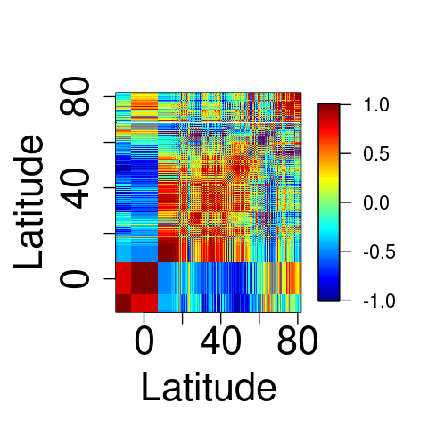
(a) Lon:$[-180^{\circ},-90^{\circ})$

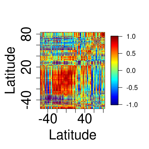
(b) Lon:$[-90^{\circ},0^{\circ})$

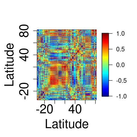
(c) Lon:$[0^{\circ},90^{\circ})$

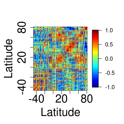
(d) Lon:$[90^{\circ},180^{\circ}]$

Figure 1: Auto-correlation plots for DU residuals across four longitude strips $[-180^{\circ},-90^{\circ})$, $[-90^{\circ},0^{\circ})$, $[0^{\circ},90^{\circ})$, $[90^{\circ},180^{\circ}]$. All symmetric about y = x.

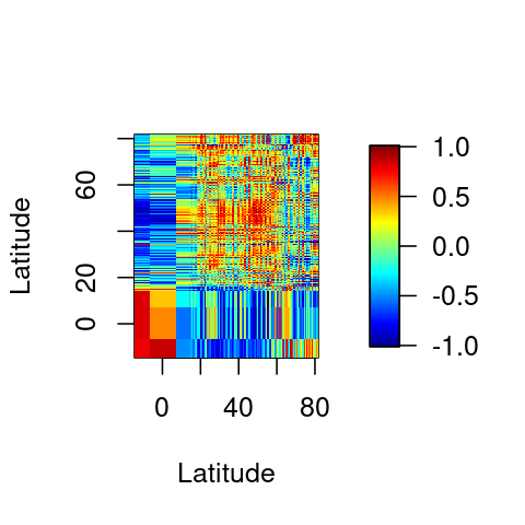
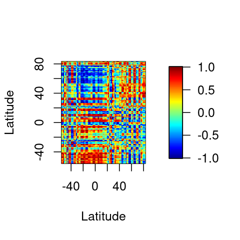
Figure 2: Cross-correlation plots for DU and SU residuals across four longitude strips $[-180^{\circ},-90^{\circ})$, $[-90^{\circ},0^{\circ})$, $[0^{\circ},90^{\circ})$, $[90^{\circ},180^{\circ}]$. All asymmetric.

In contrast, Figure 2 is the empirical spatial cross-correlation matrices for DU and SU residuals for the same four longitudinal strips. Apart from the changing patterns along with the longitude and latitude, these cross-correlation plots are asymmetric. Mathematically, $corr(DU(\textbf{s}_{1}),SU(\textbf{s}_{2}))\neq corr(DU(\textbf{s}_{2}),SU(\textbf{s}_{1}))$. This means that the cross-correlation between DU in one location, e.g., sub-Sahara and SU in another location, e.g., Saudi Arabia is not the same as the cross-correlation between DU in Saudi Arabia and SU in sub-Sahara.

Figure 2 reveals the existence of extensive spatial cross-correlations between pairs of pollutants in the spatial domain $\mathcal{D}$. However, such cross-correlation matrices only capture bivariate spatial correlations. A wealth of scientific evidence suggests that cross-correlations may exist beyond bivariate pollutants.

[23] shows that DU enhances the mass concentration of coarse SU by more than an order of magnitude; BC is the result of incomplete combustion of fossil fuels, which is usually associated with SU [26]; 45 to 55 weight per cent of OM is carbon [5]; OM tends to mix into SS and influences the final result of SS during crystallisation processes [30]; and DU frequently becomes mixed into SS during their transport in the marine boundary layer [35].

The above scientific evidence suggests that cross-correlations exist not only among bivariate pairs of pollutants but also among multiple pollutants. The CAMS reanalysis data is not just bivariate but highly multivariate.

The above evidence also implies that the interaction of pollutants associated with one particular pollutant is only confined to a small subset. More concretely, given DU and SS, BC only interacts with SU and OM. Or, equivalently, given SU and OM, BC is conditionally independent of DU and SS. Conditional independence (CI) exists among these pollutants.

In summary, the data set features highly multivariate (HM), high spatial dimensionality (HD), and asymmetric cross-covariance or cross-correlation between different pairs of pollutants across the spatial domain. Scientific evidence also suggests the existence of CI among pollutants.

Thus, the main task is to construct a valid joint covariance and/or precision matrix that reflects the above features as much as possible.

2 Introduction

So far, some literature has addressed partial facets of the features of HMHD spatial data. [24] proposed a conditional approach to model the desired joint precision matrix ($\scalebox{1.5}{$\Sigma$}_{np\times np}^{-1}$).

Under Gaussian data assumption, denote the vector $\mathbf{Y}(s_{i})$ of $p$ variates at location $s_{i}$ as $\mathbf{Y}_{i}$, where $\mathbf{Y}_{i}\in\mathbb{R}^{p}$, and the desired joint distribution as $\mathbf{Y}=[\mathbf{Y}_{1}^{\prime},\mathbf{Y}_{2}^{\prime},\cdots,\mathbf{Y}_{n}^{\prime}]^{\prime}$. By modelling each $\mathbf{Y}_{i}$ conditionally as

$$\mathbb{E}[\mathbf{Y}_{i}|\mathbf{Y}_{-i}] =\bm{\mu}_{i}+\sum_{j\in\mathcal{N}(i)}\bm{\beta}_{ij}(\mathbf{Y}_{i}-\bm{\mu}_{j}),\quad(\bm{\beta}_{ii}=-I)$$

$$Var[\mathbf{Y}_{i}|\mathbf{Y}_{-i}] =\mathbf{\Gamma}_{i},$$

then the desired joint distribution for $\mathbf{Y}=[\mathbf{Y}_{1}^{\prime},\mathbf{Y}_{2}^{\prime},\cdots,\mathbf{Y}_{n}^{\prime}]^{\prime}$ following Gaussian has the first and second moments as

$$\bm{\mu} =[\bm{\mu}_{1}^{\prime},\bm{\mu}_{2}^{\prime},\cdots,\bm{\mu}_{n}^{\prime}]^{\prime}\quad\in\mathbb{R}^{np}$$

$$\scalebox{1.5}{$\Sigma$}^{-1} =\{\mbox{block diag}(\mathbf{\Gamma}_{i})^{-1}\}\{\mbox{block}(-\bm{\beta}_{ij})\}\quad\in\mathbb{R}^{np\times np},$$

provided the symmetric condition $\bm{\Gamma}_{i}^{-1}\bm{\beta}_{ij}=\bm{\beta}_{ji}^{\prime}\bm{\Gamma}_{j}^{-1}$ and the positive definite (PD) condition that $[\mbox{block}(-\bm{\beta}_{ij})]$ being PD are satisfied.

Since $\mathbf{Y}(s_{i})\triangleq\mathbf{Y}_{i}\in\mathbb{R}^{p}$ is a whole row of the data table for the HMHD spatial data, we call this conditional approach “row-wise conditional”. Schematic representation for this “row-wise conditional”, see Figure 3(a).

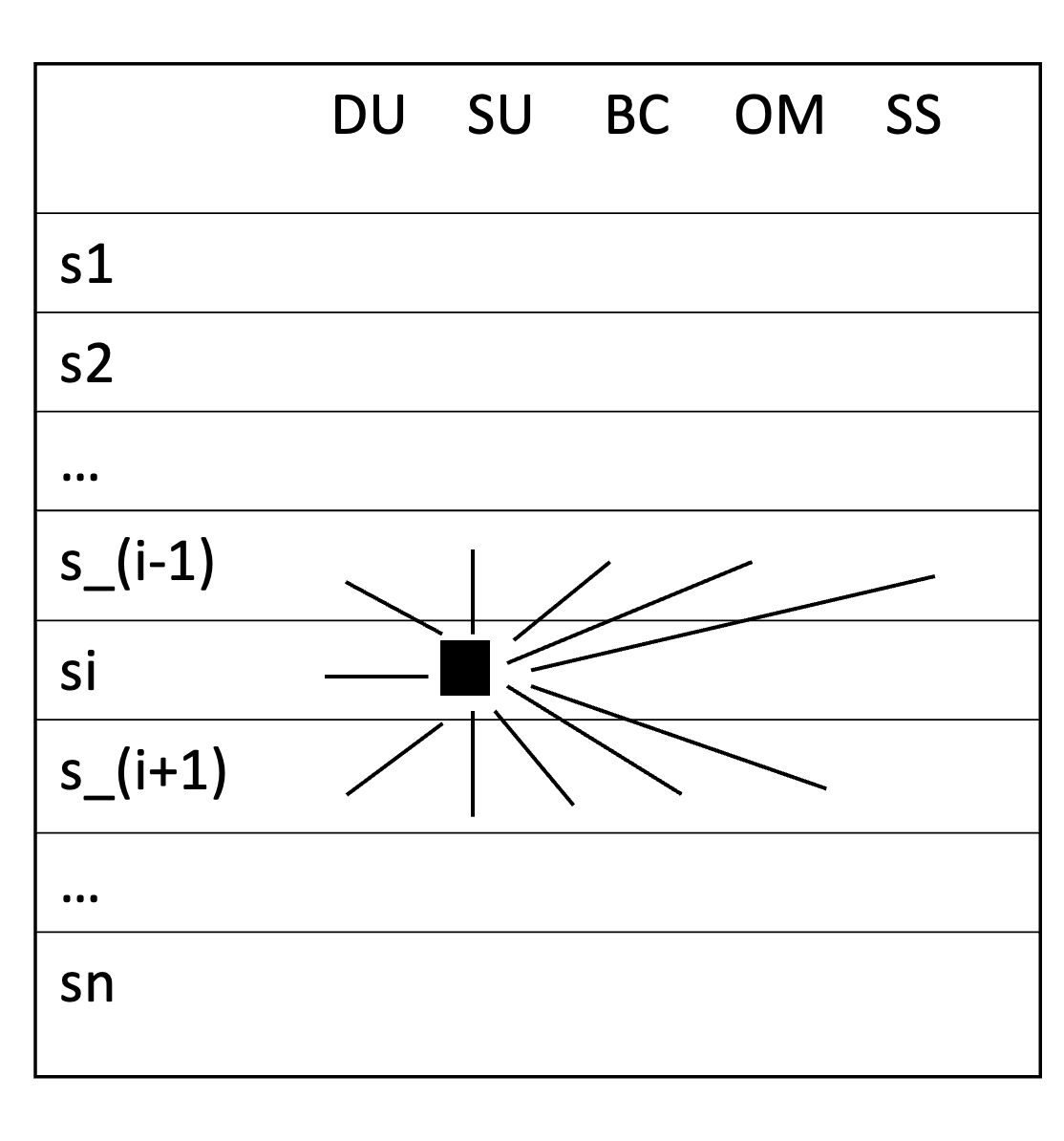
(a) Row-wise conditional

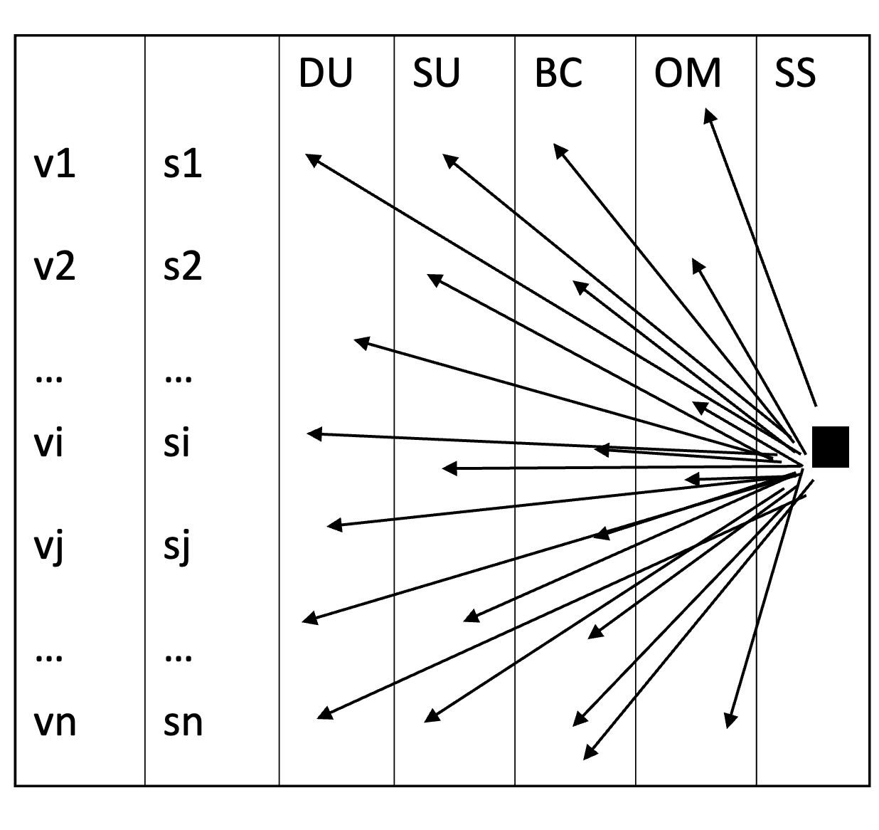
(b) Col-wise conditional

Figure 3: Schematic representations for row-wise conditional and col-wise conditional method. Row-wise conditional only regresses on neighbourhood locations but across all variates, while col-wise conditional regresses on all the previous variates across all spatial locations.

The advantage of this conditional method is that one directly obtains the desired joint precision matrix $\scalebox{1.5}{$\Sigma$}^{-1}_{np\times np}$, providing convenience for further inference of the Gaussian likelihood without the necessity to inverse from $\scalebox{1.5}{$\Sigma$}_{np\times np}$. Additionally, since the conditional mean is regressed only on neighbourhood locations, the obtained $\scalebox{1.5}{$\Sigma$}^{-1}_{np\times np}$ naturally embodies structural sparsity due to the conditional independence (CI) among spatial locations.

The disadvantages are that first, $p$ variates have to be treated as a whole, and there is no utilisation of CI among these $p$ variates; second, there is no address for the asymmetric cross-covariance existing in the off-diagonal blocks of the joint covariance matrix $\scalebox{1.5}{$\Sigma$}_{np\times np}$ due to its fundamental modelling object is $\scalebox{1.5}{$\Sigma$}^{-1}_{np\times np}$.

[8] proposed an alternative conditional modelling scheme. Instead of obtaining $\scalebox{1.5}{$\Sigma$}^{-1}_{np\times np}$, it obtains the joint covariance matrix $\scalebox{1.5}{$\Sigma$}_{np\times np}$.

Assuming Gaussian data, denote $Y_{q}(s)$ as the variate $q$ at location $s$, and vector $\bm{Y}_{r}(\cdot)$ as the variate $r$ across all spatial locations within the spatial domain $\mathcal{D}$, where $\bm{Y}_{r}(\cdot)\in\mathbb{R}^{n}$, hence a process or a variate filed. By modelling the conditional mean of $Y_{q}$ and the covariance of $Y_{q}$ about its conditional mean as,

$$\mathbb{E}(Y_{q}(s)|\{\bm{Y}_{r}(\cdot):r=1,2,\cdots,(q-1)\}) =\sum_{r=1}^{(q-1)}\int_{D}b_{qr}(s,v)Y_{r}(v)dv;\quad s\in\mathcal{D},$$ (1)

$$cov(Y_{q}(s),Y_{q}(u)|\{\bm{Y}_{r}(\cdot):r=1,2,\cdots,(q-1)\}) =C_{q|(r<q)}(s,u);\quad s,u\in\mathbb{R},$$ (2)

one obtains $\scalebox{1.5}{$\Sigma$}_{np\times np}$. The logic of obtaining the joint covariance from conditional mean and covariance dates back as early as in [34], also in [4, p. 370-372 ].

Since $\bm{Y}_{r}(\cdot)\in\mathbb{R}^{n}$ is a whole column of the data table of the HMHD spatial data, we call this conditional as “column-wise conditional”, denoted as “col-wise conditional”. For schematic representation, see Fig 3(b).

The advantage of this “col-wise conditional” is that since one obtains $\scalebox{1.5}{$\Sigma$}_{np\times np}$ directly, in the conditional mean model, through the incorporation of integro-difference equation (IDE) $\int_{D}b_{lk}(s_{i},v)y_{k}(v)dv$, a common technique in population ecology [7, p. 393], one can model the asymmetric cross-covariance directly through the function $b_{lk}(s_{i},v)$.

However, there are several shortcomings of this “col-wise conditional” method. First, from the equation (1), we notice that it requires one to sum over all the previous $(q-1)$ processes (or variate fields) when modelling the conditional mean for the $q^{th}$ variate. This means that if there were 100 processes, then one would need to sum up all the previous 99 processes, which is not scalable for the highly multivariate (HM) setting. It does not take into account the CI among $p$ variates, resulting in wasteful dynamic memory allocation and storage. In the following sections, we will see that such a method requiring a sum over all previous processes will only be appropriate for one particular instance of general graph structures, i.e., fully connected.

Second, this method constructs $\scalebox{1.5}{$\Sigma$}_{np\times np}$ directly instead of $\scalebox{1.5}{$\Sigma$}^{-1}_{np\times np}$. However, it is the latter an imperative part of the Gaussian likelihood for practical inference. This typically requires a further inversion step to obtain the $\scalebox{1.5}{$\Sigma$}^{-1}_{np\times np}$. [8] adopts Cholesky inversion, which has a dominant computational order of $\mathcal{O}(n^{3}p^{3})$ due to the $\scalebox{1.5}{$\Sigma$}_{np\times np}$ having no sparsity in general. In an HMHD spatial setting, such an inversion is exorbitantly expensive and thus prohibitive.

Third, in addition to overlooking the CI among $p$ variates, it does not consider the CI among $n$ spatial locations as the “row-wise conditional” method did in [24].

[8, Section. 4.3 ] quickly referenced graphical model representations for multivariate models, citing two examples [28] and [32]. However, [28] only addresses a bivariate scenario, and [32] is essentially a traditional canonical method and does not embody any formal graphical definitions.

[10] formally proposed a graphical model for spatial data using a pure undirected graph (UDG). However, it only addresses the highly multivariate feature without mentioning the sizeable spatial location (HD) feature. In addition, their definition of graph nodes seems to neglect the natural feature of the HMHD spatial data set, defining graph nodes only according to variates and then using strong products to “cast” them onto the spatial domain.

We respect the natural features of the HMHD spatial data set and provide our definitions for the graph nodes, edges, and graph structure. Instead of using the pure UDG structure, we propose a hybrid mixed spatial graph. Meanwhile, we innovate new concepts, such as cross-neighbour and cross-Makov Random Field (cross-MRF). Altogether, these enable a mixed conditional approach, such that both the CI among $p$ variate fields and CI among $n$ spatial locations can be taken into account simultaneously, presenting the sparsest possible representation of the $\scalebox{1.5}{$\Sigma$}_{np\times np}^{-1}$, resulting in the lowest possible computational order for inference.

What’s more, the associated algorithm will generate both $\scalebox{1.5}{$\Sigma$}_{np\times np}$ and $\scalebox{1.5}{$\Sigma$}_{np\times np}^{-1}$ in parallel, with economical dynamical memory storage for the generation of $\scalebox{1.5}{$\Sigma$}_{np\times np}$ and linear order in $p$, square order in $n$ for the generation of $\scalebox{1.5}{$\Sigma$}_{np\times np}^{-1}$ rather than $\mathcal{O}(n^{3}p^{3})$ using Cholesky inversion, presenting the lowest possible $\scalebox{1.5}{$\Sigma$}_{np\times np}$ and $\scalebox{1.5}{$\Sigma$}_{np\times np}^{-1}$ generation order.

The concurrent generation of $\scalebox{1.5}{$\Sigma$}_{np\times np}$ and $\scalebox{1.5}{$\Sigma$}_{np\times np}^{-1}$ also allows for the direct modelling of asymmetric cross-covariance in the $\scalebox{1.5}{$\Sigma$}_{np\times np}$ rather than sacrificing the opportunity to address the asymmetric cross-correlation feature by modelling $\scalebox{1.5}{$\Sigma$}_{np\times np}^{-1}$ only as in [24].

In Section 3, we formally define the mixed spatial graph. Section 4 presents the first-stage mixed spatial graphical model accounting for the CI among $p$ variates. The algorithm for generating $\scalebox{1.5}{$\Sigma$}_{np\times np}$ and $\scalebox{1.5}{$\Sigma$}_{np\times np}^{-1}$ concurrently is in Section 4.2. Section 5 includes a simulation for a six-field graph. In Section 6, we keep pursuing the possibility of accommodating the CI among $n$ spatial locations on top of the CI among $p$ variates. This includes the derivation of the cross-MRF and its conditions. In Section 7, we link the derived cross-MRF and the proposed mixed spatial graph to realise the desired CI among $p$ variates and $n$ spatial locations simultaneously, essentially, a mixed conditional modelling approach. Section 8 introduces an open problem and our proposed method as a potential solution. In Section 9, we compare different conditional modelling strategies from different facets. In Section 10, we present two illustrations using simulated and real-world data. We end this paper in Section 11, mentioning the future work.

3 Formal Definitions of Mixed Spatial Graph

To realise the mixed conditional modelling method, we first need to define a mixed spatial graph. This section presents the formal definitions for the mixed spatial graph, including nodes, edges, and graphs. Definitions of directed graph, parent nodes ($Pa(\cdot)$), child nodes ($Ch(\cdot)$), directed acyclic graph (DAG), undirected graph (UDG), and the partially directed acyclic graph (PDAG) follow the conventions of [19, p. 34-36 ].

Definition 1 (Nodes of the spatial graph).

A node in a spatial graph $\mathcal{G}$ is the $q^{th}$ variate at location $s_{i}$. It is a random quantity, a node of a probabilistic graph, and is denoted as $Y_{q}(s_{i})$, where $q=1,2,\cdots,k,\cdots,l,\cdots,p$, and $i=1,2,\cdots,n$.

Definition 2 (Variate field).

A collection of nodes for a given variate, for instance, $k$, across all spatial locations in domain $\mathcal{D}$ is called a variate field and is denoted as $\bm{Y}_{k}(\cdot)$.

Definition 3 (Spatial graph — directed).

If variate $k$ is a parent of variate $l$, that is, $k\in Pa(l)$, then for any location $s\in\mathcal{D}$, any nodes in the variate field $\bm{Y}_{k}(\cdot)$ are all parent nodes to $\bm{Y}_{l}(\cdot)$, and likewise, any nodes in the variate field $\bm{Y}_{l}(\cdot)$ are all child nodes to $\bm{Y}_{k}(\cdot)$. In particular, nodes in $\bm{Y}_{k}(\cdot)$ are all parent nodes to $Y_{l}(s)$, and nodes in $\bm{Y}_{l}(\cdot)$ are all child nodes to $Y_{k}(s)$, $s\in\mathcal{D}$. See Figure 4(a) for an illustration.

Definition 4 (Spatial graph — undirected).

For a given variate field, for instance, $\bm{Y}_{k}(\cdot)$, each node within this variate field shares equal status. That is, there are no parent or child nodes relative to each other, and any two nodes within this field, denoted as $Y_{k}(s)$ and $Y_{k}(u)$, where $s,u\in\mathcal{D}$, are neighbours and are all connected by undirected edges. See Figure 4(b) for an illustration.

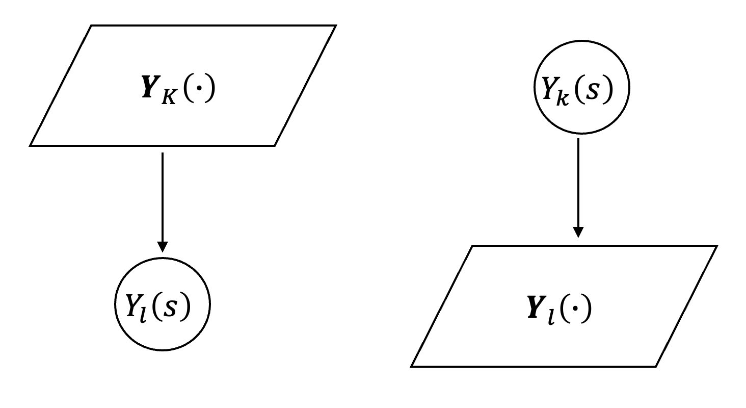
(a) Spatial graph – directed

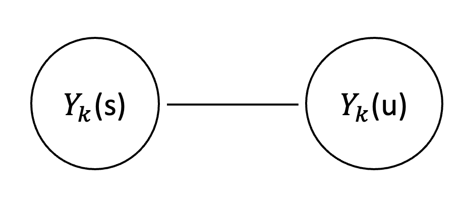
(b) Spatial graph – undirected

Figure 4: Schematic representations for directed and undirected spatial graphs. In (a), the parallelogram represents a variate field, and the circle represents one particular node in the spatial graph. They are connected by a directed edge due to the variate $k\in Par(l)$. In (b), two nodes within the same variate field $\bm{Y}_{k}(\cdot)$ are connected by an undirected edge. They are neighbours.

Definition 5 (Clique).

If every pair of nodes within a subset $\mathcal{Y}$ of nodes $\{Y_{q}(s_{i}):q=1,2,\cdots,k,\cdots,l,\cdots,p;i=1,2,\cdots,n\}$ of the graph $\mathcal{G}$ are connected by some edges (directed or undirected), then the subset $\mathcal{Y}$ of nodes is called a clique [19, p. 35]. A single node forms a singleton clique.

Definition 6 (Mixed spatial graph).

Within a single variate field $\bm{Y}_{k}(\cdot)$, the collection of nodes $\{Y_{k}(s_{i})$, $i=1,2,\cdots,n\}$ can be conceptualised as a partial realisation from a continuous field by discretisation and are all connected by undirected edges, hence consisting of an undirected spatial graph. Meanwhile, across different variate fields, i.e., $\bm{Y}_{k}(\cdot)$ and $\bm{Y}_{l}(\cdot)$, nodes within different fields are connected by directed edges, hence consisting of a directed spatial graph. Altogether, they consist of a mixed spatial graph. See Fig 5 for illustration.

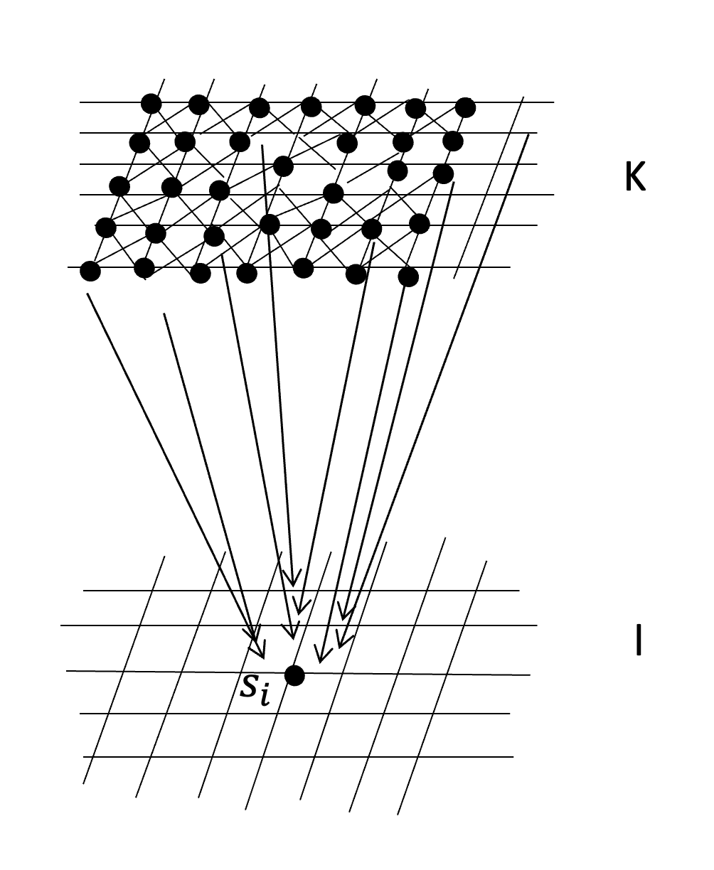
Figure 5: Illustration of a mixed spatial graph. Within a variate field $\bm{Y}_{k}(\cdot)$, all nodes share equal status and are connected by undirected edges, hence an undirected spatial graph; while across different variate fields $\bm{Y}_{k}(\cdot)$ and $\bm{Y}_{l}(\cdot)$, they are connected by directed edges, hence a directed spatial graph. Altogether, they consist of a mixed spatial graph.

It is the joint distribution of all these nodes in the mixed spatial graph of interest to us. Given the nature of continuous data, their joint distribution is assumed to be Gaussian. And the second moment of the joint Gaussian distribution, i.e., the joint variance-covariance matrix $\scalebox{1.5}{$\Sigma$}_{np\times np}$ and/or the joint precision matrix $\scalebox{1.5}{$\Sigma$}_{np\times np}^{-1}$, is of our particular modelling interest.

4 Mixed Spatial Graphical Model

4.1 The first-stage model: CI among p Variate Fields

Let $Y_{l}(s_{i})$ be a random node variable representing variate $l$ at location $s_{i}\in\mathbb{R}^{d}$, where $l=1,2,\ldots,p$, follows a topological ordering scheme, and $i=1,2,\ldots,n$. $[s_{1},s_{2},\ldots,s_{n}]^{\prime}\subseteq Domain\;\mathcal{D}\subset\mathbb{R}^{d}$. $\bm{Y}_{l}(\cdot)$ is the random field of variate $l$ across all spatial locations in $\mathcal{D}$.

By [17, p. 401-410 ], if $[\bm{Y}_{k}^{\prime}(\cdot),\bm{Y}_{l}^{\prime}(\cdot)]^{\prime}$ are jointly Normal, that is, $[\bm{Y}_{k}^{\prime}(\cdot),\bm{Y}_{l}^{\prime}(\cdot)]^{\prime}\sim\textit{Gau}(\bm{\mu}_{np\times 1},\scalebox{1.5}{$\Sigma$}_{np\times np})$, where $k=\{1,2,\ldots,r\}$, $l=\{(r+1),\ldots,p\}$, then the conditional distribution $[\bm{Y}_{l}(\cdot)|\bm{Y}_{k}(\cdot)=\bm{y}_{k}(\cdot)]$ of $\bm{Y}_{l}(\cdot)$ is also Normal, given the realisations $\{y_{k}(s_{i}):i=1,2,\ldots,n\}$ of the random nodes $\{Y_{k}(s_{i}):i=1,2,\ldots,n\}$.

The primary focus of the modelling is on $\scalebox{1.5}{$\Sigma$}_{np\times np}$ and $\scalebox{1.5}{$\Sigma$}_{np\times np}^{-1}$. The approach adopted involves iteratively (or step-wisely) deriving these matrices from the moments of conditional distribution $[\bm{Y}_{l}(\cdot)|\bm{Y}_{k}(\cdot)=\bm{y}_{k}(\cdot)]$. The method of obtaining joint $\scalebox{1.5}{$\Sigma$}_{np\times np}$ from conditional moments dates back to [34], and has also been further studied in works such as [29, 4].

The mean $\mathbb{E}[\bm{Y}_{l}(\cdot)|\bm{Y}_{k}(\cdot)=\bm{y}_{k}(\cdot)]$ of the conditional distribution and its variance $Var[\bm{Y}_{l}(\cdot)|\bm{Y}_{k}(\cdot)=\bm{y}_{k}(\cdot)]$ are modelled as follows.

For locations $\{s_{i}:i=1,2,\ldots,n\}$ in the domain $\mathcal{D}$, let $l=\{p\}$, $k=\{1,2,\ldots,(p-1):k\in Pa(l)\}$,

$$\mathbb{E}[Y_{l}(s_{i})|\bm{Y}_{k}(\cdot)=\bm{y}_{k}(\cdot)]=\mu_{l}(s_{i})+\sum_{k\in Pa(l)}\int_{\mathcal{D}}b_{lk}(s_{i},v)[y_{k}(v)-\mu_{k}(v)]dv,$$ (3)

where $\mu_{l}(s_{i})$ is the unconditional mean $\mathbb{E}[Y_{l}(s_{i})]$ and $\mu_{k}(v)$ is the unconditional mean $\mathbb{E}[Y_{k}(v)]$.

The integro-diffrence equation (IDE) $\int_{D}b_{lk}(s_{i},v)y_{k}(v)dv$ is from the textbook [7, p. 393 ], which is a technique commonly seen in population ecology, see [20, 21].

Notice two things: first, though the underlying spatial process is continuous, this IDE, in practice, will be a summation of a collection of discretised locations. Second, the integration is defined over the entire domain $\mathcal{D}$. Such an IDE is employed only for the first-stage model, and more alterations will come in the following stages.

The covariance of the conditional distribution between variate $l$ at observation location $s_{i}$ and variate $l$ at location $s_{j}$ is,

$$cov[Y_{l}(s_{i}),Y_{l}(s_{j})|\bm{Y}_{k}(\cdot)=\bm{y}_{k}(\cdot)]=\varphi_{l|k}(s_{i},s_{j}),\qquad k\in Pa(l)$$

Therefore, we have a regression equation for $Y_{l}(s_{i})$ as

$$Y_{l}(s_{i})=\mu_{l}(s_{i})+\sum_{k\in Pa(l)}\int_{\mathcal{D}}b_{lk}(s_{i},v_{i})[y_{k}(v_{i})-\mu_{k}(v_{i})]dv_{i}+\varphi_{l|k}^{\frac{1}{2}}(s_{i},s_{j})Z_{l}(s_{i}),\quad Z_{l}(s_{i})\sim N(0,1)$$ (4)

The $b_{lk}(s_{i},v_{i})$ is a regression coefficient regressing the node $Y_{l}(s_{i})$ onto node $Y_{k}(v_{i})$ while holding the rest regressors constant. $l=\{p\}$, $k\in Pa(l),k=\{1,2,\ldots,(p-1)\}$, and $i=\{1,2,\ldots,n\}$.

Lemma 1.

$b_{ll}(s_{i},s_{i})=0$ due to no self-node regression.

To obtain the $\scalebox{1.5}{$\Sigma$}_{np\times np}$, we vectorise $Y_{l}(s_{i})$ from two directions: one is within each variate $l$, vectorising over every observation locations $[s_{1},s_{2},\ldots,s_{n}]^{\prime}$, and the other is vectorising over all variates $[1,2,\ldots,p]^{\prime}$, then the vectorised regression equation corresponding to (4) is

$$\bm{Y}_{np\times 1}=\bm{\mu}_{np\times 1}+\mathcal{B}_{np\times np}(\bm{Y}_{np\times 1}-\bm{\mu}_{np\times 1})+\bm{S}_{np\times np}\bm{Z}_{np\times 1},\quad\bm{Z}\stackrel{{\scriptstyle\text{iid}}}{{\sim}}\mathcal{N}(\bm{0},\bm{I}_{np\times np}),$$ (5)

where $\mathcal{B}$ = $\scalebox{1.5}[1.5]{$[$}block[b_{lk}(\cdot,\cdot)]\scalebox{1.5}[1.5]{$]$}$ $\triangleq$ $\scalebox{1.5}[1.5]{$[$}\bm{B}_{lk}(\cdot,\cdot)\scalebox{1.5}[1.5]{$]$}$, in which $block[b_{lk}(\cdot,\cdot)]\triangleq\bm{B}_{lk}(\cdot,\cdot)$ is an $n\times n$ block matrix of $b_{lk}$ spanning across all the locations $s_{1},\ldots,s_{n}$, symbolled by $(\cdot,\cdot)$; $\bm{D}=diag\scalebox{1.5}[1.5]{$[$}block[\varphi_{l|k}(\cdot,\cdot)]\scalebox{1.5}[1.5]{$]$}$, is an $np\times np$ diagonal block matrix, with each component block matrix being $block[\varphi_{l|k}(\cdot,\cdot)]$ on the main diagonal, so the first diagonal block is $block[\varphi_{11}(\cdot,\cdot)]$, the second is $block[\varphi_{2|1}(\cdot,\cdot)]$, etc.; $\bm{S}=\bm{D}^{\frac{1}{2}}$.

Lemma 2.

The desired $\scalebox{1.5}{$\Sigma$}_{np\times np}$ is

$$\scalebox{1.5}{$\Sigma$}_{np\times np}=Var[\bm{Y}]=(\bm{I}-\mathcal{B})^{-1}\bm{D}(\bm{I}-\mathcal{B})^{-T}.$$ (6)

Proof.

See appendix A. ∎

We present in Theorem 1 a graph-structure-guided induction formula for highly multivariate (HM) spatial fields.

Theorem 1 (Graph-guided Induction Formula for $\scalebox{1.5}{$\Sigma$}_{np\times np}$).

Let $l=\{j+1\}$, $k=\{1,2,\ldots,j:k\in Pa(l)\}$. The desired $\scalebox{1.5}{$\Sigma$}_{np\times np}$ can be obtained by the below induction formula: $\scalebox{1.5}{$\Sigma$}_{np\times np}=$

$$\left[\begin{array}[]{cc}\bm{\Sigma}_{\{1,\cdots,j\}\{1,\cdots,j\}}(\cdot,\cdot)&\bm{\Sigma}_{\{1,\cdots,j\}\{1,\cdots,j\}}(\cdot,\cdot)\bm{B}_{\{j+1\}\{1,\cdots,j\}}^{T}(\cdot,\cdot)\\ \bm{B}_{\{j+1\}\{1,\cdots,j\}}(\cdot,\cdot)\bm{\Sigma}_{\{1,\cdots,j\}\{1,\cdots,j\}}(\cdot,\cdot)&\bm{B}_{\{j+1\}\{1,\cdots,j\}}\bm{\Sigma}_{\{1,\cdots,j\}\{1,\cdots,j\}}\bm{B}_{\{j+1\}\{1,\cdots,j\}}^{T}+\bm{D}_{\{j+1\}\{j+1\}}(\cdot,\cdot)\end{array}\right]$$ (9)

Proof.

See Appendix B ∎

The first subscript indicates the row index of block matrix $\bm{\Sigma}$ for different variate fields, e.g., from variate 1 to $j$; the second subscript indicates the column ones. $(\cdot,\cdot)$ indicates spanning over all spatial locations.

From this formula, we can obtain the desired $\scalebox{1.5}{$\Sigma$}_{np\times np}$ for any $p$ variate fields, meanwhile taking advantage of the CI relationship among them.

When $j=1$, the desired $\scalebox{1.5}{$\Sigma$}_{2n\times 2n}$ is

$$\scalebox{1.5}{$\Sigma$}_{2n\times 2n} =\left[\begin{array}[]{cc}\bm{\Sigma}_{\{1\}\{1\}}(\cdot,\cdot)&\bm{\Sigma}_{\{1\}\{1\}}(\cdot,\cdot)\bm{B}_{\{2\}\{1\}}^{T}(\cdot,\cdot)\\ \bm{B}_{\{2\}\{1\}}(\cdot,\cdot)\bm{\Sigma}_{\{1\}\{1\}}(\cdot,\cdot)&\bm{B}_{\{2\}\{1\}}(\cdot,\cdot)\bm{\Sigma}_{\{1\}\{1\}}(\cdot,\cdot)\bm{B}_{\{2\}\{1\}}^{T}(\cdot,\cdot)+\bm{D}_{\{2\}\{2\}}(\cdot,\cdot)\end{array}\right]$$

$$=\left[\begin{array}[]{cc}\bm{\Sigma}_{11}(\cdot,\cdot)&\bm{\Sigma}_{11}(\cdot,\cdot)\bm{B}_{21}^{T}(\cdot,\cdot)\\ \bm{B}_{21}(\cdot,\cdot)\bm{\Sigma}_{11}(\cdot,\cdot)&\bm{B}_{21}(\cdot,\cdot)\bm{\Sigma}_{11}(\cdot,\cdot)\bm{B}_{21}^{T}(\cdot,\cdot)+\bm{D}_{22}(\cdot,\cdot)\end{array}\right].$$

Obtain the desired $\scalebox{1.5}{$\Sigma$}_{3n\times 3n}$ for a tri-variate process by setting $j=2$, and obtain the desired $\scalebox{1.5}{$\Sigma$}_{4n\times 4n}$ for a four-variate process by setting $j=3$, and so forth.

Note that when beyond a bivariate setting, e.g., $j=2$, we have $\scalebox{1.5}{$\Sigma$}_{3n\times 3n}=$

$$\left[\begin{array}[]{cc}\bm{\Sigma}_{\{1,2\}\{1,2\}}(\cdot,\cdot)&\bm{\Sigma}_{\{1,2\}\{1,2\}}(\cdot,\cdot)\bm{B}_{\{3\}\{1,2\}}^{T}(\cdot,\cdot)\\ \bm{B}_{\{3\}\{1,2\}}(\cdot,\cdot)\bm{\Sigma}_{\{1,2\}\{1,2\}}(\cdot,\cdot)&\bm{B}_{\{3\}\{1,2\}}(\cdot,\cdot)\bm{\Sigma}_{\{1,2\}\{1,2\}}(\cdot,\cdot)\bm{B}_{\{3\}\{1,2\}}^{T}(\cdot,\cdot)+\bm{D}_{\{3\}\{3\}}(\cdot,\cdot)\end{array}\right],$$

but depending on different graph structures, e.g., $1\in Pa(3)$ or $2\in Pa(3)$ or $1,2\in Pa(3)$, the $\scalebox{1.5}{$\Sigma$}_{3p\times 3p}$ can be in different formats. See the Appendix C for the detailed formulae.

In particular, when both $1,2$ are the parent of $3$, it’s a special graph structure, i.e., fully connected. Consequently, one needs to sum up all the previous variate fields; see Appendix C.

This also reminds us that the formula in equation (1) for the multivariate setting is essentially one particular case corresponding to a specific fully connected graph structure. Furthermore, the bivariate case is just one special case of the fully connected graph since one always needs to sum up all the previous variate fields, which is the only one field $\bm{Y}_{1}(\cdot)$.

What’s more, the induction formula in Theorem 1 also implies any desired $\scalebox{1.5}{$\Sigma$}_{np\times np}$ of any size can always be divided into four different blocks: the leading diagonal blocks SG, the row block $\bm{R}$ beneath SG, the column block $\bm{C}$ to the right of SG, and the bottom-right block $\bm{\Sigma}_{rr}$, i.e., $\left[\begin{array}[]{cc}\left[SG\right]&\left[\bm{C}\right]\\ \left[\bm{R}\right]&\left[\bm{\Sigma}_{rr}\right]\end{array}\right]$ .

That is, when $j=1$, $r=j+1$,

$$\scalebox{1.5}{$\Sigma$}_{2n\times 2n}=\left[\begin{array}[]{cc}\left[SG\right]&\left[\bm{C}\right]\\ \left[\bm{R}\right]&\left[\bm{\Sigma}_{rr}\right]\end{array}\right]=\left[\begin{array}[]{cc}\left[SG=\bm{\Sigma}_{11}\right]&\left[\bm{C}\right]\\ \left[\bm{R}\right]&\left[\bm{\Sigma}_{22}\right]\end{array}\right]=\left[\begin{array}[]{cc}\left[\bm{\Sigma}_{11}\right]&\left[\bm{\Sigma}_{12}\right]\\ \left[\bm{\Sigma}_{21}\right]&\left[\bm{\Sigma}_{22}=\blacksquare+\bm{D}_{22}\right]\end{array}\right],$$ (16)

where the “$\blacksquare$” denotes the $\bm{B}_{\{j+1\}\{1,\cdots,j\}}\bm{\Sigma}_{\{1,\cdots,j\}\{1,\cdots,j\}}\bm{B}_{\{j+1\}\{1,\cdots,j\}}^{T}$ in Theorem 1.

When j = 2,

$$\scalebox{1.5}{$\Sigma$}_{3n\times 3n}=\left[\begin{array}[]{cc}\left[SG\right]&\left[\bm{C}\right]\\ \left[\bm{R}\right]&\left[\bm{\Sigma}_{rr}\right]\end{array}\right]=\left[\begin{array}[]{cc}\left[SG=\bm{\Sigma}_{2n\times 2n}\right]&\left[\bm{C}\right]\\ \left[\bm{R}\right]&\left[\bm{\Sigma}_{33}\right]\end{array}\right]=\left[\begin{array}[]{cc}\left[\begin{array}[]{cc}\bm{\Sigma}_{11}&\bm{\Sigma}_{12}\\ \bm{\Sigma}_{21}&\bm{\Sigma}_{22}\end{array}\right]&\left[\begin{array}[]{c}\bm{\Sigma}_{13}\\ \bm{\Sigma}_{23}\end{array}\right]\\ \left[\begin{array}[]{cc}\bm{\Sigma}_{31}&\bm{\Sigma}_{32}\end{array}\right]&\left[\bm{\Sigma}_{33}=\blacksquare+\bm{D}_{33}\right]\end{array}\right];$$ (28)

Proposition 1 (Positive Definite Condition for $\scalebox{1.5}{$\Sigma$}_{np\times np}$).

$\scalebox{1.5}{$\Sigma$}_{np\times np}$ is positive definite if and only if $\bm{\Sigma}_{\{1,\cdots,j\}\{1,\cdots,j\}}(\cdot,\cdot)$ is positive definite and its Schur complement, i.e., $\bm{D}_{\{j+1\}\{j+1\}}(\cdot,\cdot)$ is positive definite.

Proof.

By [15, p. 244, Theorem 14.8.5; Corollary 14.8.6 ], when the leading diagonal block $\bm{\Sigma}_{\{1,\cdots,j\}\{1,\cdots,j\}}(\cdot,\cdot)\triangleq SG$ in equation (9) in Theorem 1 is positive definite, and the Schur Complement of SG, denoted as $\scalebox{1.5}{$\Sigma$}_{np\times np}/SG=\bm{\Sigma}_{\{j+1\}\{j+1\}}-\bm{R}SG^{-1}\bm{C}$, i.e.,

$$=\bm{B}_{\{j+1\}\{1,\cdots,j\}}\bm{\Sigma}_{\{1,\cdots,j\}\{1,\cdots,j\}}\bm{B}_{\{j+1\}\{1,\cdots,j\}}^{T}+\bm{D}_{\{j+1\}\{j+1\}}$$

$$-\bm{B}_{\{j+1\}\{1,\cdots,j\}}\bm{\Sigma}_{\{1,\cdots,j\}\{1,\cdots,j\}}\bm{\Sigma}^{-1}_{\{1,\cdots,j\}\{1,\cdots,j\}}\bm{\Sigma}_{\{1,\cdots,j\}\{1,\cdots,j\}}\bm{B}_{\{j+1\}\{1,\cdots,j\}}^{T}$$

$$=\bm{D}_{\{j+1\}\{j+1\}}\triangleq\bm{D}_{rr}$$ (29)

is positive definite, then $\scalebox{1.5}{$\Sigma$}_{np\times np}$ is positive definite. ∎

This means, from a theoretical perspective, when $j=1$, a bivariate process, if $\bm{\Sigma}_{11}(\cdot,\cdot)$ is positive definite (PD) and $\bm{D}_{22}(\cdot,\cdot)$ is PD, then the positive definiteness of $\scalebox{1.5}{$\Sigma$}_{2n\times 2n}$ is guaranteed; when $j=2$, a tri-variate process, if $\bm{\Sigma}_{\{1,2\}\{1,2\}}(\cdot,\cdot)$ (which is $\scalebox{1.5}{$\Sigma$}_{2n\times 2n}$, the covariance matrix for bivariate process) is PD (already), and $\bm{D}_{33}$ is PD, then the $\scalebox{1.5}{$\Sigma$}_{3n\times 3n}$ is guaranteed to be PD; and so forth.

So, for p variates, when $\bm{\Sigma}_{11}(\cdot,\cdot)$ is PD, and $\bm{D}_{22}$, $\bm{D}_{33},\ldots$, $\bm{D}_{pp}$ are all positive definite, then the positive definiteness of $\scalebox{1.5}{$\Sigma$}_{np\times np}$ is guaranteed. [29, Theorem 2 ] and [8, Section. 4.2 ] mentioned the similar idea. However, this is a theoretical result, and in actual practice, other factors, such as numerical stability, also affect the final positive definiteness due to the iterative construction process. We defer details to Section 5.2.

Theorem 2 (Construction of $\scalebox{1.5}{$\Sigma$}^{-1}_{np\times np}$).

$\scalebox{1.5}{$\Sigma$}^{-1}_{np\times np}$ can also be obtained iteratively, step by step. And such an iterative construction of $\scalebox{1.5}{$\Sigma$}^{-1}_{np\times np}$ is on the computational order $p*\mathcal{O}(n^{3})$, linear in $p$.

Proof.

By [16, p. 25, equation (0.8.5.6) ], for a given $\scalebox{1.5}{$\Sigma$}_{np\times np}$, when the inverse of its leading diagonal block SG, i.e., $SG^{-1}$, and the inverse of the Schur complement of $SG$, i.e., $(\scalebox{1.5}{$\Sigma$}_{np\times np}/SG)^{-1}=\bm{D}_{rr}^{-1}$ (see the proof in Proposition 1) are provided, the $\scalebox{1.5}{$\Sigma$}^{-1}_{np\times np}$ can be obtained using formula

$$\scalebox{1.5}{$\Sigma$}^{-1}_{np\times np}=\left[\begin{array}[]{cc}SG^{-1}[SG+\bm{C}\bm{D}_{rr}^{-1}\bm{R}]SG^{-1}&-SG^{-1}\bm{C}\bm{D}_{rr}^{-1}\\ -\bm{D}_{rr}^{-1}\bm{R}SG^{-1}&\bm{D}_{rr}^{-1}\end{array}\right]$$ (32)

So, when $j=1$,

$$\scalebox{1.5}{$\Sigma$}_{2n\times 2n}^{-1}=\left[\begin{array}[]{cc}\bm{\Sigma}_{11}^{-1}[\bm{\Sigma}_{11}+\bm{C}\bm{D}_{22}^{-1}\bm{R}]\bm{\Sigma}_{11}^{-1}&-\bm{\Sigma}_{11}^{-1}\bm{C}\bm{D}_{22}^{-1}\\ -\bm{D}_{22}^{-1}\bm{R}\bm{\Sigma}_{11}^{-1}&\bm{D}_{22}^{-1}\end{array}\right],$$

where computing $\bm{\Sigma}_{11}^{-1},\bm{D}_{22}^{-1}$ is $\mathcal{O}(n^{3})$; where computing $\bm{D}_{33}^{-1}$ is $\mathcal{O}(n^{3})$ and $\bm{\Sigma}_{2n\times 2n}^{-1}$ is already obtained from the last step, stored and can be easily fetched from memory cache; And when $j=(p-1)$,

$$\scalebox{1.5}{$\Sigma$}_{np\times np}^{-1}=\left[\begin{array}[]{cc}\bm{\Sigma}_{(p-1)n\times(p-1)n}^{-1}[\bm{\Sigma}_{(p-1)n\times(p-1)n}+\bm{C}\bm{D}_{pp}^{-1}\bm{R}]\bm{\Sigma}_{(p-1)n\times(p-1)n}^{-1}&-\bm{\Sigma}_{(p-1)n\times(p-1)n}^{-1}\bm{C}\bm{D}_{pp}^{-1}\\ -\bm{D}_{pp}^{-1}\bm{R}\bm{\Sigma}_{(p-1)n\times(p-1)n}^{-1}&\bm{D}_{pp}^{-1}\end{array}\right],$$ (35)

where computing $\bm{D}_{pp}^{-1}$ is $\mathcal{O}(n^{3})$ and $\bm{\Sigma}_{(p-1)n\times(p-1)n}^{-1}$ is already obtained from the last step, stored and easily fetched from the memory cache.

Therefore, one only needs to compute $\bm{\Sigma}_{11}^{-1}$, $\bm{D}_{22}^{-1}$, $\ldots$, $\bm{D}_{pp}^{-1}$, and each of these $n\times n$ matrix inversion is $\mathcal{O}(n^{3})$, so the total computational order is $p*\mathcal{O}(n^{3})$, which is linear in $p$. ∎

It is worth mentioning that the intensive floating point (flop) operations, such as matrix multiplications, either use the default Basic Linear Algebra Subprograms (BLAS) and LAPCK on CPU or are parallelised on GPU.

This theorem 2 indicates one could obtain the $\scalebox{1.5}{$\Sigma$}_{np\times np}^{-1}$ simultaneously as one obtains the $\scalebox{1.5}{$\Sigma$}_{np\times np}$ step-by-step, and such a construction method requires computational order only linear in $p$. In contrast to a direct inversion of $\scalebox{1.5}{$\Sigma$}_{np\times np}$, which requires $\mathcal{O}((np)^{3})$, cubic in both $p$ and $n$; or via Cholesky inversion whose Cholesky decomposition step requires $\mathcal{O}((np)^{3}/3)$ and inversion the decomposed lower triangular matrix requires $\mathcal{O}((np)^{2})$, hence the dominant order is still $\mathcal{O}((np)^{3})$.

Proposition 2 (Positive Definite Condition for $\scalebox{1.5}{$\Sigma$}^{-1}_{np\times np}$).

The $\scalebox{1.5}{$\Sigma$}^{-1}_{np\times np}$ constructed step-wisely above is positive definite if and only if $\bm{D}_{rr}^{-1}$ and $SG^{-1}$ at each iteration step $r$ are both positive definite.

Proof.

By [15, Corollary 14.8.6 ] and denote the $\scalebox{1.5}{$\Sigma$}^{-1}$ at each iteration $r$ of the form of equation (32) as $\left[\begin{array}[]{cc}BK1&BK2\\ BK3&BK4\end{array}\right]$ , then $\scalebox{1.5}{$\Sigma$}^{-1}$ at each iteration $r$ is PD iff $BK4=\bm{D}_{rr}^{-1}$ and its Schur Complement $\scalebox{1.5}{$\Sigma$}^{-1}/BK4=BK1-(BK2)(BK4^{-1})(BK3)=SG^{-1}$ are PD.

Note that $SG^{-1}$ at each $r^{th}$ iteration is essentially the $\scalebox{1.5}{$\Sigma$}^{-1}$ at $(r-1)^{th}$ iteration (see equation 35), which is already PD at the time of construction; therefore, one only needs the $SG^{-1}$ at the first iteration (i.e., $\Sigma_{11}^{-1}$) to be PD and all the BK4 at each iteration (i.e., $D_{rr}^{-1}$) being PD. ∎

Again, this is from a purely theoretical perspective. Other factors, such as numerical stability, may still impact the final positive definiteness of $\scalebox{1.5}{$\Sigma$}^{-1}$ in actual practice due to the iterative construction procedure. For details, see Section 5.2.

Theorem 3 (CI among $p$ variate fields).

For each variate field $\bm{Y}_{l}(\cdot)$, it is conditionally independent of its non-descendant fields given its parent fields. Expressed in mathematical terms,

$$\bm{Y}_{l}(\cdot)\perp\bm{Y}_{q}(\cdot)|\bm{Y}_{k}(\cdot),$$

where $\bm{Y}_{q}(\cdot)$ is the non-descendant fields of $\bm{Y}_{l}(\cdot)$, $k\in Pa(l)$.

Proof.

The CI between the field $\bm{Y}_{l}(\cdot)$ and its non-descendant fields $\bm{Y}_{q}(\cdot)$ is due to the mixed spatial graphical model structure, in which the cross fields are modelled using a Directed Acyclic Graph (DAG). By the CI property of DAG [19, p. 57], given the parent fields of $\bm{Y}_{l}(\cdot)$, it is conditionally independent of its non-descendant fields $\bm{Y}_{q}(\cdot)$.

∎

Since the CI among different fields is mathematically reflected by conditional covariance, that is, $cov(\bm{Y}_{l}(\cdot),\bm{Y}_{q}(\cdot)|\bm{Y}_{k}(\cdot))=\bm{0}$, and the conditional covariance has intrinsic connections with the joint precision matrix $\scalebox{1.5}{$\Sigma$}_{np\times np}^{-1}$, therefore, this section concludes with following conjecture:

Conjecture 1.

Such a CI between field $\bm{Y}_{l}(\cdot)$ and fields $\bm{Y}_{q}(\cdot)$ is reflected in the joint precision matrix $\scalebox{1.5}{$\Sigma$}_{np\times np}^{-1}$ in the form of exact zero-valued block matrices of dimension $n\times n$.

4.2 The algorithm

Following the rules revealed by Theorem 1 and Theorem 2, and together with given graph structures, we present the Algorithm 1 (see Appendix D) for generating the desired $\scalebox{1.5}{$\Sigma$}_{np\times np}$ for any CI structure among $p$ variate fields ($p\gg 2$) reflected by the graph and the corresponding $\scalebox{1.5}{$\Sigma$}_{np\times np}^{-1}$ simultaneously at a computational order linear in $p$.

When provided with a Directed Acyclic Graph (DAG) among $p$ variate fields, the algorithm generates the corresponding $\scalebox{1.5}{$\Sigma$}_{np\times np}$ without redundant computations or unnecessary dynamic memory allocations.

Specifically, steps 9 to 12 of the algorithm leverage the graphical parent-child relationships to involve only those pairs of variates that exhibit a conditional dependence during the computation, substantially improving the $\scalebox{1.5}{$\Sigma$}_{np\times np}$ generation efficiency. This approach also reduces the dynamic memory storage requirement from order $\mathcal{O}((pn)^{2})$ to $\mathcal{O}((qn)^{2})$, where $q$, representing the number of parent nodes, is much smaller than $p$, and $p\gg 2$. The algorithm will sum up all the previous variate fields when and only when the provided DAG is fully connected.

Meanwhile, $\scalebox{1.5}{$\Sigma$}_{np\times np}^{-1}$ is generated in parallel at a significantly reduced computational order (i.e., $p*\mathcal{O}(n^{3})$) compared to direct inversion or Cholesky inversion, both of which operate at the computational order $\mathcal{O}((pn)^{3})$. The difference in the computational order is easily observed, for instance, when $p=10$, resulting in $10*\mathcal{O}(n^{3})$ versus $1000*\mathcal{O}(n^{3})$.

Therefore, the graph-guided induction algorithm is scalable to highly multivariate (HM) spatial settings.

5 Simulation: Six Fields

Figure 6 is a randomly drawn acyclic graphical structure for six fields. The aim of this simulation is to use the theories and algorithm derived so far to generate the joint $\scalebox{1.5}{$\Sigma$}_{np\times np}$ and $\scalebox{1.5}{$\Sigma$}^{-1}_{np\times np}$ simultaneously for these six fields. Meanwhile, the positive definiteness of these two objects is ensured.

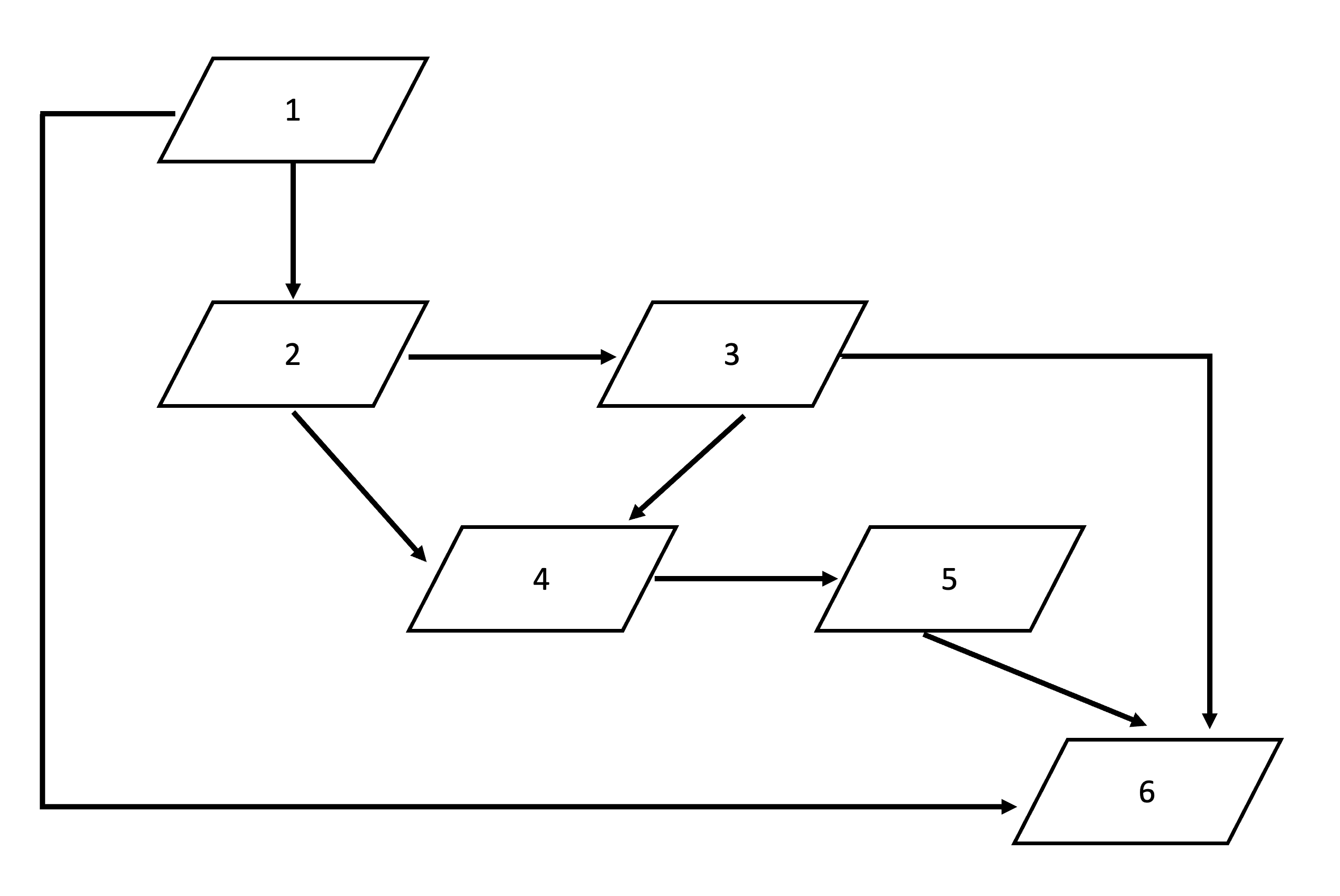
Figure 6: A randomly drawn acyclic graphical structure for six fields.

5.1 Simulation setting

For this simulation, spatial domain $\mathcal{D}=[-1,1]$ with gird size 0.05 and each location $s\in\mathbb{R}^{1}$.

Since the underlying spatial processes for the six fields are all continuous, so traditional geostatistical covariance models such as exponential or Matérn are possible choices.

For convenience, we use the Matérn function of a special form ($\nu$ = 3/2) to model all the univariate covariance $Cov((Y_{l}(s_{i}),Y_{l}(s_{j}))|Y_{k}(\cdot))$ for every single variate $l$ across all spatial locations, where $l,k=\{1,2,\ldots,p:k\in Pa(l)\}$, $i,j=\{1,2,\ldots,n\}$, that is, $\bm{\Sigma}_{11}(\cdot)$, $\bm{D}_{22}(\cdot),\ldots,\bm{D}_{66}(\cdot)$ are modelled using below Matérn:

$$Matern(d;\nu=3/2,\kappa)=\sigma^{2}(1+\kappa d)exp(-\kappa d),$$

where $d$ is the Euclidean distance between pairs of locations, and $\kappa$ is the large-scale decay parameter controlling the correlation decreasing speed; $\nu=3/2$ controls the smoothness of the function.

From Proposition 1, we know that the theoretical PD of $\scalebox{1.5}{$\Sigma$}_{np\times np}$ is ensured if $\bm{\Sigma}_{11}$, $\bm{D}_{22},\ldots,\bm{D}_{66}$ are all PD, which is guaranteed by the Matérn function provided parameter $\kappa>0$.

For convenience, we fixed all the marginal variances $\sigma^{2}$ of each Matérn to be unit 1, and all the large-scale decay parameters $\kappa$ to be 2. But they will be the inference objects in actual practice.

5.2 b function, B matrix and numerical stability

From Theorem 1 and the step 10 in algorithm 1, we know that the $\bm{B}_{rt}$ = $block[b_{rt}(\cdot,\cdot)]$, $t\in Pa(r)$ is a matrix whose element values are obtained from evaluating the function $b_{rt}(\cdot,\cdot)$ across all locations $s\in\mathcal{D}$.

[8, Section. 2 ] mentioned that such a b function could account for asymmetric cross-correlation, and they used a bisquare function with positive values only to accommodate the asymmetry. However, from the cross-correlation plots in Figure 2 in Section 1, we observe clear negative cross-correlations between pairs of variates across different spatial regions. In addition, the bisquare function for every pair of variates requires three parameters for 1D space and five for 2D space, which is not scalable for highly multivariate settings where $p\gg 2$.

Therefore, we propose a modified triangular wave function with both positive and negative functional values to better capture the actual cross-correlation while requiring fewer parameters.

The modified triangular wave has a functional form as follows,

$$Tri-Wave(h)=\left\{\begin{array}[]{rcl}A\{1-\phi(\frac{/h-\Delta/}{/\Delta/})^{2}\}&\mbox{for}&/h-\Delta/\leq\rho/\Delta/\\ 0&\mbox{for}&/h-\Delta/>\rho/\Delta/\end{array}\right.,$$ (38)

$A$ (amplitude) and $\Delta$ (horizontal translation) are two parameters obtained from inference, while $\phi$ and $\rho$ are two manually-set factors. $\phi$ controls the decay speed of the function value, and $\rho$ decides the compact support radius beyond which the function values are set to exact zero. See Appendix E for the shape of the Tri-Wave function.

When the $(i,j)^{th}$ element of the matrix $\bm{B}_{rt}$ is obtained from $b_{rt}(h_{ij};\Delta_{rt},A_{rt})$, where each $h_{ij}$ is displacement (with both direction and magnitude) instead of distance (with only magnitude) between pairs of locations, and therefore the $(i,j)^{th}$ element of the matrix $\bm{B}_{rt}$ is not equal to the $(j,i)^{th}$ element due to displacement $h_{ij}-\Delta\neq h_{ji}-\Delta$, that is, $\bm{B}_{rt}(i,j)\neq\bm{B}_{rt}(j,i)$, the asymmetric cross-correlation is accounted.

Regarding the robustness of the positive definiteness of $\scalebox{1.5}{$\Sigma$}_{np\times np}$ and $\scalebox{1.5}{$\Sigma$}^{-1}_{np\times np}$, since highly multivariate (HM) settings involve repeated multiplications of $\bm{B}_{rt}$ (i.e., $\bm{B}$ exponentiation) during the iterative $\scalebox{1.5}{$\Sigma$}_{np\times np}$ and $\scalebox{1.5}{$\Sigma$}^{-1}_{np\times np}$ construction procedures, this implies if the spectral norm of $\bm{B}_{rt}$ is greater than 1, and/or $\bm{B}_{rt}$ has a very large condition number, any unavoidable tiny errors (e.g., rounding error) associated with the floating point arithmetic [31, p. 97] in the further multiplications that involve such $\bm{B}$ exponentiation term will be magnificently amplified, thereby shattering the numerical stability and the robustness of the positive definiteness of the final $\scalebox{1.5}{$\Sigma$}_{np\times np}$ and $\scalebox{1.5}{$\Sigma$}^{-1}_{np\times np}$.

To uphold the numerical stability and the robustness of the positive definiteness of $\scalebox{1.5}{$\Sigma$}_{np\times np}$ and $\scalebox{1.5}{$\Sigma$}^{-1}_{np\times np}$, we use a combination of spectral normalisation and regularisation to control the spectral norm of $\bm{B}_{rt}$ and its condition number, a technique commonly used in deep neural network training, see [25].

We test and compare the robustness of the positive definiteness of $\scalebox{1.5}{$\Sigma$}_{np\times np}$ and $\scalebox{1.5}{$\Sigma$}^{-1}_{np\times np}$ using three versions of the modified Tri-Wave functions (V4, V5, V7) and one version of the Wendland function (see Appendix F) for $\bm{B}_{rt}$ on three combinations of grid size (ds) and domain ($\mathcal{D}$), i.e., $\{ds=0.1,\mathcal{D}=[-1,1]\}$, $\{ds=0.05,\mathcal{D}=[-1,1]\}$, $\{ds=0.1,\mathcal{D}=[-10,10]\}$ under two graph structures corresponds to two highly multivariate fields (i.e., p = 5 and p = 7). The positive definiteness is tested using 100 parameter combinations, where parameter $A$ ranges from 0.1 $\sim$ 1, and parameter $\Delta$ ranges from 0.1 $\sim$ 1, both by 0.1. The test results show a remarkable improvement in the robustness of the positive definiteness of $\scalebox{1.5}{$\Sigma$}_{np\times np}$ and $\scalebox{1.5}{$\Sigma$}^{-1}_{np\times np}$ using $\bm{B}_{rt}^{SpN+Reg}$ than those using the original $\bm{B}_{rt}^{Orinigal}$. For the full test results and analyses, see Appendix G.

5.3 Simulation results

We use one version of the modified Tri-Wave function (i.e., V5 where $\phi=2$, $\rho=1$) having both positive and negative values and one version of the Wendland function (i.e., $k=3/2$, $R=0.5$) having only positive values as the b function to construct $\bm{B}_{rt}$ matrix and thereby simulate the $\scalebox{1.5}{$\Sigma$}_{np\times np}$ and $\scalebox{1.5}{$\Sigma$}^{-1}_{np\times np}$ for six fields organised by the graph structure in Figure 6. The simulation results are displayed in Figure 7 and Figure 8, in which Figure 7 uses the original b function while Figure 8 uses the b function undergone a combination of spectral normalisation and regularisation (SpN + Reg).

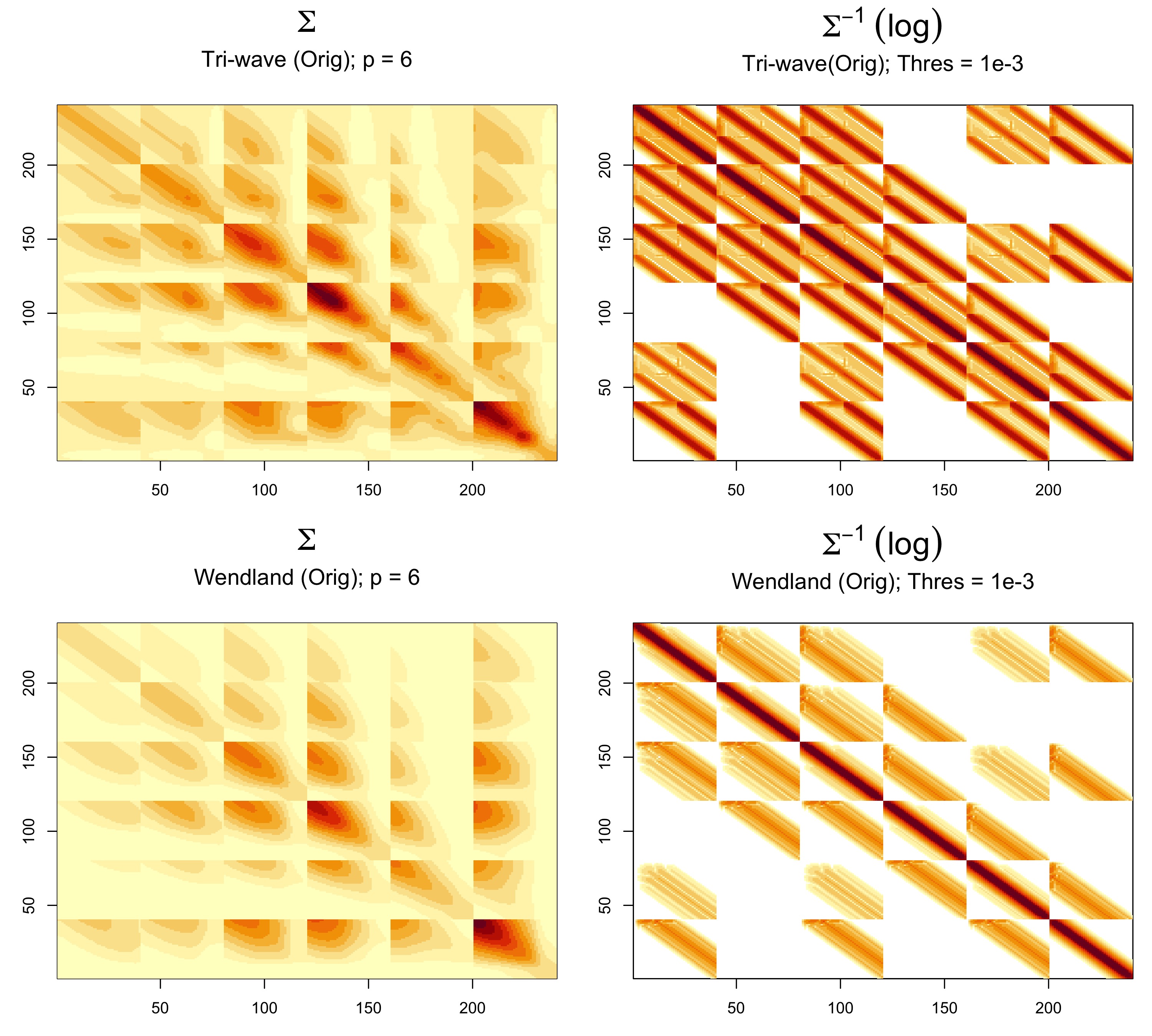
Figure 7: 1D simulation of $\Sigma$ and $\Sigma^{-1}$ for six fields. The upper panel uses the Tri-wave function, and the lower panel uses the Wendland function. In (a), both functions are on their original scale without normalisation transformation, and in (b) both are under a combination of spectral normalisation and regularisation transformation. The left figures in (a) and (b) are all $\Sigma$s, and the right ones are all $\Sigma^{-1}$s on the log scale. Parameter A = 0.1, parameter $\Delta$ = 0.5. The largest possible threshold for the values of $\Sigma^{-1}$ is $1e^{-3}$.

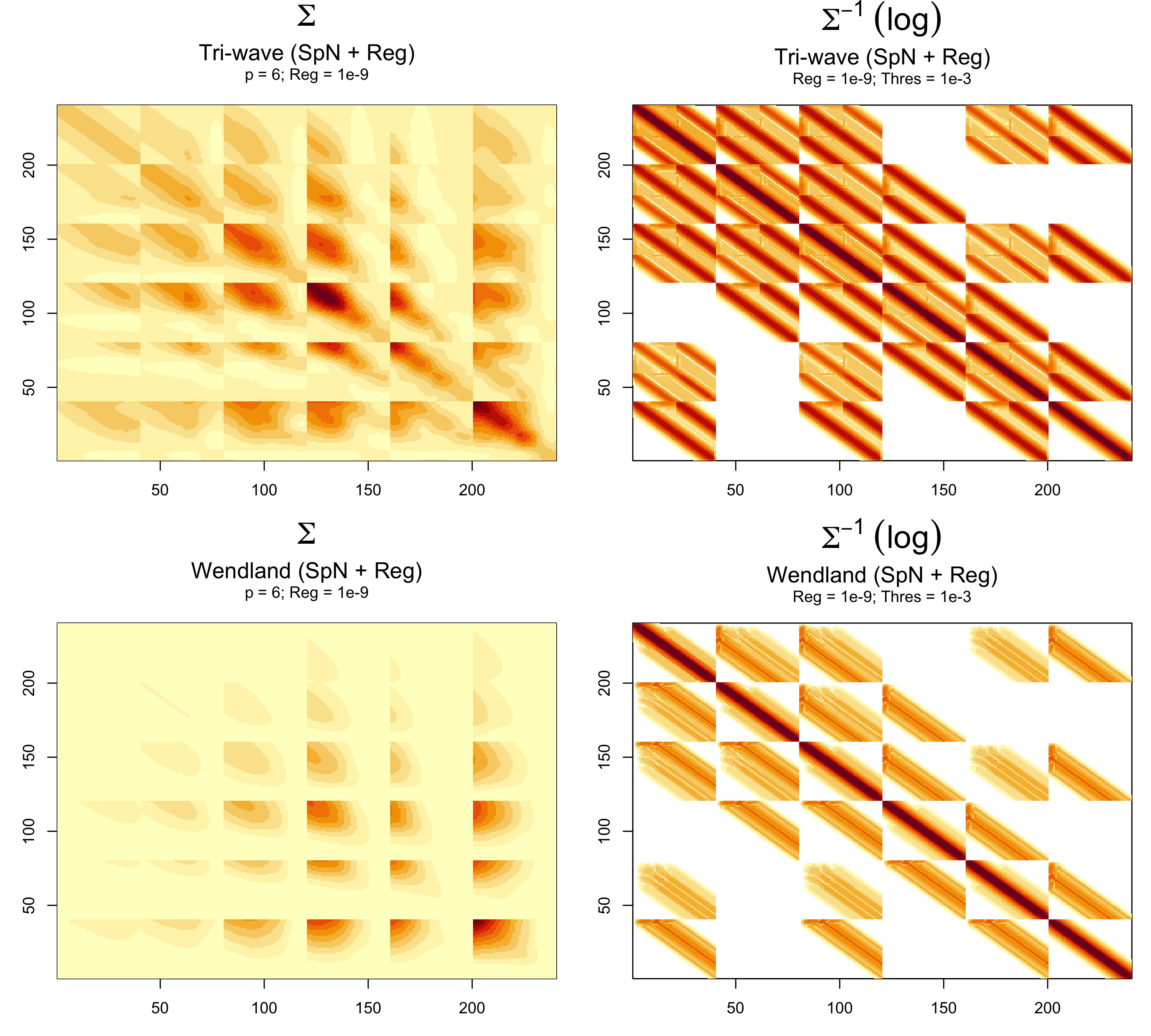
Figure 8: 1D simulation of $\Sigma$ and $\Sigma^{-1}$ for six fields. The upper panel uses the Tri-wave function, and the lower panel uses the Wendland function. Both b functions are under a combination of spectral normalisation and regularisation transformation. The left figures are $\Sigma$s, and the right ones are $\Sigma^{-1}$s on the log scale. Parameter A = 0.1, parameter $\Delta$ = 0.5. The largest possible threshold for the values of $\Sigma^{-1}$ is $1e^{-3}$. The default smallest possible regularisation number is $1e^{-9}$.

From the $\scalebox{1.5}{$\Sigma$}_{np\times np}$ plots in both Figure 7 and Figure 8 for both b functions (Tri-Wave and Wendland) on both scales (original and SpN + Reg), we observe that the diagonal blocks are all symmetric. In contrast, the off-diagonal blocks are all asymmetric. This means our observed asymmetry in the cross-covariance between different fields in Section 1 have been specifically addressed.

From the $\scalebox{1.5}{$\Sigma$}^{-1}_{np\times np}$ plots in both Figure 7 and Figure 8, we observe the sparse structures. The sparsity reflects the CI among $p$ variate fields embedded in the DAG of six fields in Figure 6. It is computationally realised through threshold the values of $\scalebox{1.5}{$\Sigma$}^{-1}_{np\times np}$, and we default the threshold to be $1e^{-3}$. It will automatically decrease to the largest possible value to ensure the $\scalebox{1.5}{$\Sigma$}^{-1}_{np\times np}$ is PD even after the threshold.

The regularisation number defaults to $1e^{-9}$ and will automatically increase until the smallest possible value is found to ensure the robustness of the PD of $\scalebox{1.5}{$\Sigma$}^{-1}_{np\times np}$.

This subsection concludes with two observations.

Observation 1.

Given the CI among $p$ variate fields embedded in the DAG of the hybrid mixed spatial graph, the joint precision matrix $\scalebox{1.5}{$\Sigma$}^{-1}_{np\times np}$ exhibits structural sparsity.

Observation 2.

The sparse structure is not entirely consistent with the CI among $p$ variate fields embedded in the DAG.

For instance, according to the CI properties of DAG, the variate field “5” shall be conditionally independent with its non-descendant fields “1”, “2”, and “3”, given its parent field “4”. However, in the joint precision matrix plots in both Figure 7 and Figure 8, field “5” is only conditionally independent of field “2”.

Answers to the second observation will be explored in the subsequent sections.

6 Beyond CI among p-Variates: Cross-MRF

So far, the graph-guided induction formula has taken advantage of the CI structure among $p$ variate fields. This has accelerated the generation of $\scalebox{1.5}{$\Sigma$}_{np\times np}$ and $\scalebox{1.5}{$\Sigma$}_{np\times np}^{-1}$ with much more cost-effective dynamic memory storage and efficient computational order (linear in $p$). In addition, the simultaneously generated $\scalebox{1.5}{$\Sigma$}_{np\times np}^{-1}$ has displayed structural sparsity. The approach up until now has brought tangible scalability to highly multivariate (HM) spatial settings.

However, such a generation order is still cubic in spatial location $n$, and whether the sparsity exhibited in $\scalebox{1.5}{$\Sigma$}_{np\times np}^{-1}$ can be further enhanced when addressing the high spatial dimensionality (HD) feature on top of the HM is worthy of probing. The further enhanced sparsity in $\scalebox{1.5}{$\Sigma$}_{np\times np}^{-1}$ may further benefit the subsequent inference of the likelihood involving $\scalebox{1.5}{$\Sigma$}_{np\times np}^{-1}$.

Therefore, we address the HD problem on top of the HM settings.

In doing so, it is questioned whether

$$\mathbb{E}[Y_{l}(s_{i})|\bm{Y}_{k}(\mathcal{N}(s_{i}))=\bm{y}_{k}(\mathcal{N}(s_{i}))]=\mu_{l}(s_{i})+\sum_{k\in Pa(l)}\int_{v\in\mathcal{N}(s_{i})}b_{lk}(s_{i},v)[y_{k}(v)-\mu_{k}(v)]dv,$$

$l=\{p\}$, $k=\{1,2,\ldots,(p-1):k\in Pa(l)\}$, instead of $\mathbb{E}[Y_{l}(s_{i})|\bm{Y}_{k}(\cdot)=\bm{y}_{k}(\cdot)]$ (see equation 3 in Section 4.1), is possible.

And this is the same question as whether this conditional $\mathbb{E}[Y_{l}(s_{i})|\bm{Y}_{k}(\mathcal{N}(s_{i}))=\bm{y}_{k}(\mathcal{N}(s_{i}))]$ instead of this conditional $\mathbb{E}[Y_{l}(s_{i})|\bm{Y}_{k}(\cdot)=\bm{y}_{k}(\cdot)]$ can still define the desired joint $[\bm{Y}_{1}^{\prime}(\cdot),\dots,\bm{Y}_{p}^{\prime}(\cdot)]^{\prime}$.

To answer this question, we resort to the Hammersley-Clifford (H-C) theorem [6].

6.1 Multivariate H-C theorem from col-wise conditional perspective

Besag (1974) proved the univariate version of the Hammersley-Clifford (H-C) theorem

$$\frac{p(\textbf{y})}{p(\textbf{x})}=\scalebox{1.5}{$\Pi$}_{i=1}^{n}\frac{p(y_{i}|y_{1},\cdots,y_{i-1},x_{i+1},\cdots,x_{n})}{(x_{i}|y_{1},\cdots,y_{i-1},x_{i+1},\cdots,x_{n})}.$$

Mardia (1988) showed the multivariate version, while the multivariate is under the row-wise conditional ideology, and the essence of the proof is vectorising $y_{i}\in\mathbb{R}^{1}$ to $\bm{y}_{i}\in\mathbb{R}^{p}$:

$$\frac{p(\textbf{y})}{p(\textbf{x})}=\scalebox{1.5}{$\Pi$}_{i=1}^{n}\frac{p(\bm{y}_{i}|\bm{y}_{1},\cdots,\bm{y}_{i-1},\bm{x}_{i+1},\cdots,\bm{x}_{n})}{(\bm{x}_{i}|\bm{y}_{1},\cdots,\bm{y}_{i-1},\bm{x}_{i+1},\cdots,\bm{x}_{n})}.$$

We show the multivariate case of the H-C theorem under a column-wise conditional mentality and obtain the below lemma:

Lemma 3 (Multivariate H-C Theorem from Col-wise Conditional Perspective).

From col-wise conditional, $p(\bm{y})=p(\bm{y}_{k}(\cdot),\bm{y}_{l}(\cdot))$ and

$$\frac{p(\bm{y}_{k}(\cdot),\bm{y}_{l}(\cdot))}{p(\bm{y}_{k}(\cdot),\bm{x}_{l}(\cdot))}=\scalebox{1.5}{$\Pi$}_{i=1}^{n}\frac{p(y_{l}(s_{i})|y_{l}(s_{1}),\cdots,y_{l}(s_{i-1}),x_{l}(s_{i+1}),\ldots,x_{l}(s_{n}),\bm{y}_{k}(\cdot))}{p(x_{l}(s_{i})|y_{l}(s_{1}),\cdots,y_{l}(s_{i-1}),x_{l}(s_{i+1}),\ldots,x_{l}(s_{n}),\bm{y}_{k}(\cdot))},$$ (39)

where $[\bm{y}_{k}(\cdot),\bm{y}_{l}(\cdot)]\in\Omega=\Omega_{k}\times\Omega_{l}$ the sample space for all possible realisations for different fields, i.e., $[\bm{y}_{k}(\cdot),\bm{y}_{l}(\cdot)]=[y_{k}(s_{1}),y_{k}(s_{2}),\ldots,y_{k}(s_{n}),y_{l}(s_{1}),y_{l}(s_{2}),\ldots,y_{l}(s_{n})]$, and $k,l$ are conditionally dependent, $l,k=\{1,\cdots,p\}$, $k\neq l$.

Proof.

See Appendix H. ∎

Note that this Lemma 3 relaxes the parent-child relationship for $k,l$ and only requires them to be conditionally dependent. We will link the general theory derived in Section 6.1, 6.2 and 6.3 with the $k,l$’s parent-child relationship of our mixed spatial graphical model framework in Section 7.

This lemma means if a given variable of a particular variate at a given location is specified with its associated neighbourhood structure, the whole system of such variables will generate a valid stochastic process.

And if we expand $\bm{y}$ as $(y_{l}(s_{1}),y_{l}(s_{2}),\cdots,y_{l}(s_{i}),\cdots,y_{l}(s_{n}),\bm{y}_{k}(\cdot))$, follow [2, Section 3 ] write $\bm{y}_{i}^{l}=(y_{l}(s_{1}),\cdots,y_{l}(s_{i-1}),0,y_{l}(s_{i+1}),\cdots,y_{l}(s_{n}),\bm{y}_{k}(\cdot))$, and define

$$Q(\bm{y})=ln\frac{p(\bm{y})}{p(\bm{0})},$$ (40)

where $p(\bm{0})>0$ (the strict positivity condition), we have an alternative view of the above H-C theorem:

Lemma 4 (Alternative View of Multivariate H-C Theorem).

$$Q(\bm{y})-Q(\bm{y}_{i}^{l})=ln\frac{p(\bm{y})}{p(\bm{y}_{i}^{l})}=ln\frac{p(y_{l}(s_{i})|y_{l}(s_{1}),\cdots,y_{l}(s_{i-1}),y_{l}(s_{i+1}),\cdots,y_{l}(s_{n}),\bm{y}_{k}(\cdot))}{p(0_{l}(s_{i})|y_{l}(s_{1}),\cdots,y_{l}(s_{i-1}),y_{l}(s_{i+1}),\cdots,y_{l}(s_{n}),\bm{y}_{k}(\cdot))},$$ (41)

This alternative H-C theorem indicates when given the neighbourhood structure of a given variable of a particular variate at a given location, in order to obtain a valid and the desired joint distribution $p(\bm{y})$, one needs to know the most general form of $Q(\bm{y})$.

Since by [4, p. 386-387 ], the desired joint distribution

$$p(\bm{y})\varpropto\scalebox{1.5}{$\Pi$}_{c}\Psi_{c}(\bm{y}_{c})\varpropto\scalebox{1.5}{$\Pi$}_{c}exp(-E(\bm{y}_{c}))=exp(-\sum_{c}E(\bm{y}_{c})),$$

where $\Psi_{c}(\cdot)$ is a potential function over clique $c$ and $\sum_{c}E(\bm{y}_{c})$ is the sum of energy of each clique $c$, therefore, $Q(\bm{y})\varpropto lnp(\bm{y})\varpropto\sum_{c}E(\bm{y}_{c})$. This means the $Q(\bm{y})$ can be expanded as a sum of energy over each clique.

To expand out the most general form of the $Q(\bm{y})$, we need three more definitions:

Definition 7 (Variable-wise singleton clique).

If $\bm{y}_{i}=(y_{1}(s_{i}),\cdots,y_{q}(s_{i}),\cdots,y_{p}(s_{i}))\in\mathbb{R}^{p}$ forms a singleton clique, as implied in [24], then each component $y_{q}(s_{i}),q=1,\cdots,p$, forms a variable-wise singleton clique.

Definition 8 (Cross-clique and cross-neighbourhood).

If $\bm{y}_{i}$ and $\bm{y}_{j}$, each $\in\mathbb{R}^{p}$, form a clique, then $y_{l}(s_{i})$ and $y_{k}(s_{j})$ form a clique as well, and we name such a clique as a cross-clique, the neighbourhood formed by $y_{l}(s_{i})$ and $y_{k}(s_{j})$ is called cross-neighbourhood, in which $k,l$ are conditionally dependent and $s_{j}\in\mathcal{N}(s_{i})$. See the left figure in Figure 9(a) for an illustration.

Definition 9 (Auto-clique and auto-neighbourhood).

If $\bm{y}_{i}$ and $\bm{y}_{j}$, each $\in\mathbb{R}^{p}$, form a clique, then $y_{l}(s_{i})$ and $y_{l}(s_{j})$ form an auto-clique, and the neighbourhood formed by $y_{l}(s_{i})$ and $y_{l}(s_{j})$ is called auto-neighbourhood. See the right figure in Figure 9(b).

(a) Cross-neighbourhood

(b) Auto-neighbourhood

Figure 9: Illustration of cross-neighbourhood formed by $y_{l}(s_{i})$ and $y_{k}(s_{j})$ and auto-neighbourhood formed by $y_{l}(s_{i})$ and $y_{l}(s_{j})$. Variates $k,l$ are conditionally dependent, and $s_{j}\in\mathcal{N}(s_{i})$.

With these definitions, we can write out the expansion of $Q(\bm{y})$ in terms of G-functions,

$$Q(\bm{y})=\sum_{l=1}^{p}\sum_{i=1}^{n}y_{l}(s_{i})G_{i}^{l}(y_{l}(s_{i}))+\sum_{l=1}^{p}\sum_{1\leq i,j\leq n}^{n}y_{l}(s_{i})y_{l}(s_{j})G_{i,j}^{l,l}(y_{l}(s_{i}),y_{l}(s_{j}))+\cdots+\sum_{l=1}^{p}y_{l}(s_{1})y_{l}(s_{2})\cdots y_{l}(s_{i})\cdots y_{l}(s_{n})G_{1,2,\cdots,n}^{l,l,\ldots,l}(\cdot)+\sum_{1\leq k,l\leq p}\sum_{1\leq i,j\leq n}y_{l}(s_{i})y_{k}(s_{j})G_{i,j}^{l,k}(y_{l}(s_{i}),y_{k}(s_{j}))+\ldots+\sum_{1\leq k,l\leq p}y_{k}(s_{1})y_{k}(s_{2})\ldots y_{k}(s_{i-1})y_{l}(s_{i})y_{k}(s_{i+1})\ldots y_{k}(s_{n})G_{1,2,\ldots,(i-1),i,(i+1),\ldots,n}^{k,k,\ldots,k,\quad,l,\quad,k,\dots,k}(\cdot),$$ (42)

and if denote $\bm{y}_{i}^{l}\triangleq(y_{l}(s_{1}),y_{l}(s_{2}),\ldots,y_{l}(s_{i-1}),0,y_{l}(s_{i+1}),\ldots,y_{l}(s_{n}),\bm{y}_{k}(\cdot))$, we have

$$Q(\bm{y})-Q(\bm{y}_{i}^{l})=y_{l}(s_{i})G_{i}^{l}(y_{l}(s_{i}))+\sum_{1\leq j\leq n}^{n}y_{l}(s_{i})y_{l}(s_{j})G_{i,j}^{l,l}(y_{l}(s_{i}),y_{l}(s_{j}))+\cdots+y_{l}(s_{1})y_{l}(s_{2})\cdots y_{l}(s_{i})\cdots y_{l}(s_{n})G_{1,2,\cdots,n}^{l,l,\ldots,l}(\cdot)+\sum_{1\leq k\leq p}\sum_{1\leq j\leq n}y_{l}(s_{i})y_{k}(s_{j})G_{i,j}^{l,k}(y_{l}(s_{i}),y_{k}(s_{j}))+\ldots+\sum_{1\leq k\leq p}y_{k}(s_{1})y_{k}(s_{2})\ldots y_{k}(s_{i-1})y_{l}(s_{i})y_{k}(s_{i+1})\ldots y_{k}(s_{n})G_{1,2,\ldots,(i-1),i,(i+1),\ldots,n}^{k,k,\ldots,k,\quad,l,\quad,k,\dots,k}(\cdot).$$ (43)

And $Q(\bm{y})-Q(\bm{y}_{i}^{l})$ will depend on $y_{l}(s_{j})$ only when $y_{l}(s_{i})$ and $y_{l}(s_{j})$ form an auto-clique, that is $s_{j}\in\mathcal{N}(s_{i})$; and will depend on $y_{k}(s_{j})$ only when $y_{l}(s_{i})$ and $y_{k}(s_{j})$ form a cross-clique, that is $k,l$ are conditionally dependent meanwhile $s_{j}\in\mathcal{N}(s_{i})$.

These are equivalent to say only when either the auto G-function $y_{l}(s_{i})y_{l}(s_{j})G_{i,j}^{l,l}$ or cross G-function $y_{l}(s_{i})y_{k}(s_{j})G_{i,j}^{l,k}$ is non-null.

The non-null auto G-function and cross G-function can, in turn, further simplify the equation (41) in Lemma 4 to

$$Q(\bm{y})-Q(\bm{y}_{i}^{l})=ln\frac{p(y_{l}(s_{i})|y_{l}(s_{j}),y_{k}(s_{j}),\{0_{r}(s_{h}):h\neq i,j;r\neq k,l\})}{p(0_{l}(s_{i})|y_{l}(s_{j}),y_{k}(s_{j}),\{0_{r}(s_{h}):h\neq i,j;r\neq k,l\})},$$ (44)

where $s_{j}\in\mathcal{N}(s_{i})$, $k,l$ are conditionally dependent and $0_{l}(s_{i})$ denotes $y_{l}(s_{i})=0$.

On the other hand, by equation (43) and (44), the auto and cross G-functions can be expressed in terms of $Q(\bm{y})$ and therefore conditional probabilities.

They are the G functions that reflect variable-wise singleton clique:

$$y_{l}(s_{i})G_{i}^{l}(y_{l}(s_{i})) =Q(0,\cdots,0,y_{l}(s_{i}),0,\cdots,0)-Q(\textbf{0})$$

$$=ln\frac{p(y_{l}(s_{i})|\{0_{r}(s_{h}):h\neq i;r\neq l\})}{p(0_{l}(s_{i})|\{0_{r}(s_{h}):h\neq i;r\neq l\})},$$ (45)

reflect auto-clique:

$$y_{l}(s_{i})y_{l}(s_{j})G_{i,j}^{l,l}(y_{l}(s_{i}),y_{l}(s_{j}))=Q(0,\cdots,0,y_{l}(s_{i}),0,\cdots,0,y_{l}(s_{j}),0,\cdots,0)-Q(0,\cdots,0,\underline{0},0,\cdots,0,y_{l}(s_{j}),0,\cdots,0)-Q(0,\cdots,0,y_{l}(s_{i}),0,\cdots,0,\underline{0},0,\cdots,0)+Q(\textbf{0})\\ =ln\frac{p(y_{l}(s_{i})|y_{l}(s_{j}),\{0_{r}(s_{h}):h\neq i,j;r\neq l\})}{p(0_{l}(s_{i})|y_{l}(s_{j}),\{0_{r}(s_{h}):h\neq i,j;r\neq l\})}-ln\frac{p(y_{l}(s_{i})|\{0_{r}(s_{h}):h\neq i;r\neq l\})}{p(0_{l}(s_{i})|\{0_{r}(s_{h}):h\neq i;r\neq l\})},$$ (46)

and reflect cross-clique:

$$y_{l}(s_{i})y_{k}(s_{j})G_{i,j}^{l,k}(y_{l}(s_{i}),y_{k}(s_{j}))=Q(0,\cdots,0,y_{l}(s_{i}),0,\cdots,0,y_{k}(s_{j}),0,\cdots,0)-Q(0,\cdots,0,\underline{0},0,\cdots,0,y_{k}(s_{j}),0,\cdots,0)-Q(0,\cdots,0,y_{l}(s_{i}),0,\cdots,0,\underline{0},0,\cdots,0)+Q(\textbf{0})\\ =ln\frac{p(y_{l}(s_{i})|y_{k}(s_{j}),\{0_{r}(s_{h}):h\neq i,j;r\neq l,k\})}{p(0_{l}(s_{i})|y_{k}(s_{j}),\{0_{r}(s_{h}):h\neq i,j;r\neq l,k\})}-ln\frac{p(y_{l}(s_{i})|\{0_{r}(s_{h}):h\neq i;r\neq l\})}{p(0_{l}(s_{i})|\{0_{r}(s_{h}):h\neq i;r\neq l\})}$$ (47)

The above series of reasoning implies that from the specification of conditional distributions, we can obtain auto and cross G-functions (by equations (46) and (47)), from these G-functions we can obtain $Q(\bm{y})$ (by equation (42)), and from $Q(\bm{y})$ we could obtain our desired joint distribution $p(\bm{y})$ (by equation (40)).

This means that from those conditional distributions that reflect auto and cross-neighbourhood structures, we could arrive at our desired joint $p(\bm{y})$. Or equivalently, this conditional $\mathbb{E}[Y_{l}(s_{i})|\bm{Y}_{k}(\mathcal{N}(s_{i}))=\bm{y}_{k}(\mathcal{N}(s_{i}))]$, instead of this conditional $\mathbb{E}[Y_{l}(s_{i})|\bm{Y}_{k}(\cdot)=\bm{y}_{k}(\cdot)]$, can still define the desired joint $[\bm{Y}_{1}^{\prime}(\cdot),\dots,\bm{Y}_{p}^{\prime}(\cdot)]^{\prime}$, should certain conditions are satisfied.

6.2 Conditions and verifications

In general, the conditions are (a) strict positivity condition: $p(\bm{y})>0$ for $\forall\bm{y}\in\Omega$; in particular, $p(\bm{0})>0$; (b) $\int_{\bm{y}\in\Omega}exp(Q(\bm{y}))<\infty$; and (c) auto G-functions and cross G-functions are symmetric, i.e., (i) $y_{l}(s_{i})y_{l}(s_{j})G_{i,j}^{l,l}=y_{l}(s_{j})y_{l}(s_{i})G_{j,i}^{l,l}$; (ii) $y_{l}(s_{i})y_{k}(s_{j})G_{i,j}^{l,k}=y_{k}(s_{j})y_{l}(s_{i})G_{j,i}^{k,l}$.

The first condition means the joint distribution of all the processes $\bm{Y}$’s is strictly positive. In particular, there exists a positive probability that all the realisations of all the processes $\bm{Y}$’s can be zero. This ensures the definition of $Q(\bm{y})$ in equation (40) is valid.

The second condition is to ensure the desired joint distribution $p(\bm{y})$ exists and is a valid probability distribution that sums up to 1, which is satisfied via an appropriate normalizing constant of $Q(\bm{y})$.

The third condition is to ensure the obtained variance-covariance or precision matrix for the joint $p(\bm{y})$ following the exponential family is symmetric.

Due to the propagation relationship between G-functions, $Q(\bm{y})$, the joint distribution $p(\bm{y})$ and conditional distributions, this third condition is fulfilled via the partial regression coefficient $b(\cdot,\cdot)$ in the conditional means $\mathbb{E}[Y_{l}(s_{i})|\bm{Y}_{k}(\mathcal{N}(s_{i}))=\bm{y}_{k}(\mathcal{N}(s_{i}))]$ and $\mathbb{E}[Y_{l}(s_{i})|\bm{Y}_{l}(\mathcal{N}(s_{i}))=\bm{y}_{l}(\mathcal{N}(s_{i}))]$. Specifically, for auto G-functions, their invariance is equivalent to require $b_{ll}(s_{i},s_{j})=b_{ll}(s_{j},s_{i})$, and for cross G-functions, it is equivalent to require $b_{lk}(s_{i},s_{j})=b_{kl}(s_{j},s_{i})$.

By the meaning of partial regression coefficients, $b_{ll}(s_{i},s_{j})=b_{ll}(s_{j},s_{i})$ indicates the equivalence between regressing $Y_{l}(s_{i})$ on $Y_{l}(s_{j})$ and the reverse while controlling the rest of variables (or graph nodes). This is trivial as spatial locations of one particular variate $l$ are modelled using undirected graphs; hence, they must be symmetric.

Follow the same ideology, $b_{lk}(s_{i},s_{j})=b_{kl}(s_{j},s_{i})$ implies not only that variate $l$ and $k$ are conditionally dependent (hence regressing on each other) but also that they are in a symmetric relationship. The verification and the realisation of this condition are detailed in Section 7.

6.3 Cross-MRF

In a univariate setting, the univariate spatial stochastic process $\{Y(s_{i}):i=1,2,\ldots,n\}$ is a (univariate-) Markov Random Field when the univariate conditional distributions $\{[Y(s_{i})|Y(\mathcal{N}(s_{i}))]:i=1,2,\ldots,n\}$ can define a univariate joint distribution $\bm{Y}(\cdot)$ [7, p. 176].

Analogue to the above univariate case, the cross-Markov Random Field for the multivariate case is presented below.

Definition 10 (Cross-MRF).

When the conditions in Section 6.2 are satisfied, the cross-conditional distributions $\{[Y_{l}(s_{i})|Y_{k}(\mathcal{N}(s_{i}))]:l,k=1,\ldots,p;k\not\perp l|Rest;k\sim l;i=1,2,\ldots,n\}$ together with the auto-conditional distributions $\{[Y_{l}(s_{i})|Y_{l}(\mathcal{N}(s_{i}))]:l=1,2,\ldots,p;i=1,2,\ldots,n\}$, can define the desired joint distribution $p(\bm{y})$. Therefore, the multivariate spatial stochastic process $\{Y_{l}(s_{i}),Y_{k}(s_{i}):l,k=1,2,\ldots,p;i=1,2,\ldots,n\}$ is a cross Markov Random Field (cross-MRF). Here, $k\not\perp l|Rest$ means $k,l$ are conditionally dependent given the rest; $k\sim l$ means $k,l$ are symmetric, and $p\in\mathbb{Z}^{+}$, $p\geq 2$; $k\neq l$.

So the cross-MRF features variates $k$, $l$ being conditionally dependent and in a symmetric relationship, and $s_{j}\in\mathcal{N}(s_{i})$. The “cross” here refers to both the $n$ spatial locations (row-wise conditional) and $p$ variates (col-wise conditional) enjoying the CI simultaneously.

Further, given the relationship between $p(\bm{y})$ and $Q(\bm{y})$ in equation 40, the relationship between $Q(\bm{y})$ and G-functions in equation 42, and the relationship between G-functions and conditional probabilities in equation 6.1, 46, 47, it is straightforward to obtain

$$p(\bm{y})\varpropto\prod_{l=1}^{p}\prod_{i=1}^{n}[y_{l}(s_{i})]\times\prod_{l=1}^{p}\prod_{i=1}^{n}[y_{l}(s_{i})|y_{l}(\mathcal{N}(s_{i}))]\times\prod_{1\leq k,l\leq p}\prod_{1\leq i\leq n}[y_{l}(s_{i})|y_{k}(\mathcal{N}(s_{i}))],$$ (48)

where $p\in\mathbb{Z}^{+}$, $p\geq 2$; $k\neq l$.

This means the desired joint probability $p(\bm{y})$ can be expressed as a product of variable-wise singleton cliques, auto-cliques, and cross-cliques. See Appendix I for detailed verification.

The Table 10 in Appendix J presents a comparison of different facets between the MRF for univariate spatial processes and the cross-MRF for multivariate spatial processes.

7 Linking Cross-MRF with Mixed Spatial Graphical Framework

Knowing the conditions and features of the cross-MRF, our question now narrows down to how to realise these conditions within the mixed spatial graphical framework such that both the CI among $p$ variates and the CI among $n$ locations can be enjoyed and reflected in the $\scalebox{1.5}{$\Sigma$}_{np\times np}^{-1}$ to benefit further the subsequent inference on top of the solo CI among $p$ variate fields.

7.1 Realising symmetric G-functions

From Section 6.2, we know that the auto-G and cross-G function’s symmetry is required for cross-MRF and are fulfilled via partial regression coefficients in the conditional means. More concretely, for auto G-functions, we require $b_{ll}(s_{i},s_{j})=b_{ll}(s_{j},s_{i})$, and for cross G-functions, we require $b_{lk}(s_{i},s_{j})=b_{kl}(s_{j},s_{i})$.

$b_{ll}(s_{i},s_{j})=b_{ll}(s_{j},s_{i})$ is satisfied in the mixed spatial graphical framework because each univariate field $\bm{Y}_{l}(\cdot)$ across all spatial locations $s\in\mathcal{D}$ is modelled using an undirected graph (UDG), i.e., $Y_{l}(s_{i})$ and $Y_{l}(s_{j})$ are in a symmetric relationship, hence $b_{ll}(s_{i},s_{j})=b_{ll}(s_{j},s_{i})$ is satisfied.

$b_{lk}(s_{i},s_{j})=b_{kl}(s_{j},s_{i})$ not only reflects that $k$ and $l$ are conditionally dependent, but also implies a symmetric relationship between $Y_{l}(s_{i})$ and $Y_{k}(s_{j})$. Since the relationship between locations is modelled using UDG and is therefore symmetric by nature, it only remains to find a symmetric relationship between variates $l$ and $k$.

In the mixed spatial graphical framework, cross-variate fields are initially modelled using a directed acrylic graph (DAG). This means we need to obtain a symmetric relationship between variates $l$ and $k$ within a directed graph framework. Meanwhile, the CI structures specified by the DAG among cross-variate fields are fully preserved.

Normally, the graph structure that realises the symmetry between $k$ and $l$ is the UDG. This indicates to obtain the desired symmetry between variates, we need to transform our original DAG among the cross-variate fields to an undirected one while the original CI encoded in the DAG remains intact.

We, therefore, give the sufficient and necessary condition to realise $b_{lk}(s_{i},s_{j})=b_{kl}(s_{j},s_{i})$ in the mixed spatial graphical model framework.

Proposition 3.

$b_{lk}(s_{i},s_{j})=b_{kl}(s_{j},s_{i})$ is realised in the mixed spatial graphical model framework if and only if the directed acrylic graph which models the cross-variate fields are moral. That is, the mixed spatial graphical framework has no “unmarried” parent fields for a commonly shared child field. Any “unmarried” parent fields will be “married” using undirected edges.

Proof.

Sufficiency. By Proposition 4.8, 4.9 in [19, p. 135 ], a moralised DAG can be converted to its corresponding undirected graph without losing its conditional independence.

Necessity. If the DAG is not moral, then $k$ and $l$ will have a parent-child relationship with only one particular direction, contradicting the symmetric relation. ∎

Corollary 1.

If the DAG in the mixed spatial graphical model framework is chain-structured, $b_{lk}(s_{i},s_{j})=b_{kl}(s_{j},s_{i})$ must be realised.

Proof.

See Appendix K. ∎

Detailed moralisation steps include “marrying” the parent fields that share a common child field using undirected edges. Meanwhile, all the arrows of directed edges in the graph are dropped. After moralisation, such a moralised mixed graph then becomes an undirected graph (see definition 4.19 in [19, p. 148 ]). And follow the definition 4.20 in [19, p. 149 ], if associate a potential factor $\psi(\cdot)$ to each chain-component of the mixed spatial graph (i.e., a partially directed graph), then the equation (48) can be further written as proportionate to a product of three types of potential functions $\psi(\cdot)$, where each conditional distribution is absorbed into one clique potential, capturing the interaction of nodes within auto-cliques and cross-cliques. That is,

$$p(\bm{y})\varpropto\prod_{l=1}^{p}\prod_{i=1}^{n}\psi(y_{l}(s_{i}))\times\prod_{l=1}^{p}\prod_{i=1}^{n}\psi(y_{l}(s_{i}),y_{l}(\mathcal{N}(s_{i})))\times\prod_{1\leq k,l\leq p}\prod_{1\leq i\leq n}\psi(y_{l}(s_{i}),y_{k}(\mathcal{N}(s_{i}))),$$ (49)

where $p\in\mathbb{Z}^{+}$, $p\geq 2$; $k\neq l$.

As a matter of fact, the singleton cliques $y_{l}(s_{i})$ can be additionally absorbed into the auto-cliques. Therefore, the above equation 49, can be further modified to

$$p(\bm{y})\varpropto\prod_{l=1}^{p}\prod_{i=1}^{n}\psi(y_{l}(s_{i}),y_{l}(\mathcal{N}(s_{i})))\times\prod_{1\leq k,l\leq p}\prod_{1\leq i\leq n}\psi(y_{l}(s_{i}),y_{k}(\mathcal{N}(s_{i}))).$$ (50)

These two products are multiplied in a way that matches their common part “$y_{l}(s_{i})$” and is essentially a factorisation over the mixed spatial graph, comprising the auto-cliques and cross-cliques. See Figure 10 for an illustration.

Figure 10: Schematic representations for the joint distribution factorising over the mixed spatial graph, comprising auto-cliques and cross-cliques.

7.2 Realising $s_{j}\in\mathcal{N}(s_{i})$

To realise another feature of cross-MRF, i.e., $s_{j}\in\mathcal{N}(s_{i})$, recall our spatial graphical framework is a mixed one, with pairs of cross fields represented by DAGs, while each univariate field represented by UDGs.

This reminds us that instead of directly modelling the univariate covariance matrices ( i.e., $\bm{\Sigma}_{11}$, $\bm{D}_{22}$, $\ldots,\bm{D}_{pp}$) using geostatistical process covariance models such as Matérn, see step 1 and step 16 in the Algorithm 1, we could use the lattice process covariance model, i.e., conditional autoregressive (CAR) [2, Section. 4.2] to model the inverse of the univariate covariance matrices (i.e., $\bm{\Sigma}_{11}^{-1}$, $\bm{D}_{22}^{-1}$, $\ldots,\bm{D}_{pp}^{-1}$). And for the generation of $\scalebox{1.5}{$\Sigma$}_{np\times np}$ that requires the univariate covariance matrices, we only need to invert each of the $\bm{\Sigma}_{11}^{-1}$, $\bm{D}_{22}^{-1}$, $\ldots,\bm{D}_{pp}^{-1}$ back. See the modified Algorithm 2 in Appendix L.

The advantage of modelling directly the inverse of the univariate covariance matrix using CAR during the construction of $\scalebox{1.5}{$\Sigma$}^{-1}$ is that the required $\bm{\Sigma}_{11}^{-1}$, $\bm{D}_{22}^{-1}$, $\ldots,\bm{D}_{pp}^{-1}$ is ready-made and no need to inverse them from the univariate covariance matrices, hence exempt from the computational order $p*\mathcal{O}(n^{3})$ mentioned in Theorem 2, and only remains basic matrix multiplications using BLAST and LAPACK and very easy to be parallelised on GPUs. Meanwhile, for the generation of $\Sigma$ , one only needs to inverse back the modelled inverse of the univariate covariance matrices at the computational order of $p*O(n)$, linear in both $p$ and $n$, due to the banded structure of (univariate) MRF obtained under CAR models. In addition, parameter estimation is usually easier using univariate CAR than using a geostatistical model, e.g., Matérn [3, Section. 1].

Explicitly, model $\bm{\Sigma}_{11}^{-1}$ and $\bm{D}_{22}^{-1}$ directly using CAR, that is $\bm{\Sigma}_{11}^{-1}=(\bm{I}-\phi\bm{H})\bm{M}_{1}^{-1}$, and $\bm{D}_{22}^{-1}=(\bm{I}-\phi\bm{H})\bm{M}_{2}^{-1}$, where $\bm{H}=[h_{ij}]$ is a matrix encodes spatial neighbourhood adjacency information, with $h_{ij}=1$ if $s_{j}\in\mathcal{N}(s_{i})$ and $h_{ij}=0$ if $s_{j}\notin\mathcal{N}(s_{i})$; $\phi$ reflects the proportion of spatial dependence on the neighbouring values modelled in the conditional mean [1, p. 82]; $\bm{M}$ is often re-parametrised as the product of marginal variance $\sigma^{2}_{11}$ or $\sigma^{2}_{22}$ and identity matrix $\bm{I}$, that is $\bm{M}_{1}=\sigma^{2}_{11}\bm{I}$ or $\bm{M}_{2}=\sigma^{2}_{22}\bm{I}$.

The only condition required is to ensure the inverse of the univariate covariance matrix (i.e., $\bm{\Sigma}_{11}^{-1}$, $\bm{D}_{22}^{-1}$, $\ldots,\bm{D}_{pp}^{-1}$) to be positive definite (PD) so that each of the univariate covariance matrix itself (i.e., $\bm{\Sigma}_{11}$, $\bm{D}_{22}$, $\ldots,\bm{D}_{pp}$) is PD, such that the desired joint $\scalebox{1.5}{$\Sigma$}_{np\times np}^{-1}$ is PD (by Proposition 2) and the desired joint $\scalebox{1.5}{$\Sigma$}_{np\times np}$ is PD (by Proposition 1).

Such a condition is achieved through the spectral radius of $\phi\bm{H}$ being less than 1. That is, $\phi$ is capped by the inverse of the maximum absolute eigenvalue of $\bm{H}$, resulting in all the eigenvalues of $(I-\phi\bm{H})$ being positive; hence, $(I-\phi\bm{H})$ is PD, see [14, p. 82 ]. To achieve reasonable spatial correlation among neighbouring sites, this parameter $\phi$ is usually chosen to be close to the upper boundary of its parameter space [3, Section 1].

An alternative method to the above modelling the inverse of univariate covariance matrices using CAR (univariate MRF) is to direct modelling the univariate covariance matrices $\bm{\Sigma}_{11}$, $\bm{D}_{22}$, $\dots$, $\bm{D}_{pp}$ using the geostatistical covariance matrix, e.g., Matérn or exponential, then to realise $s_{j}\in\mathcal{N}(s_{i})$, one uses a tapering function to taper the univariate geostatistical covariance, such that the resulting covariance matrices are sparse; see [13].

The $s_{j}\in\mathcal{N}(s_{i})$ is reflected by the tapered kernel function, with elements being exactly zero when $\parallel s_{j}-s_{i}\parallel>\alpha$, where $\alpha$ is a particular scalar.

The common choice for the tapering function is from the Wendland family [33, 13], such as the Wendland 1 (k = 3/2) function $WL_{1}(h)$ we mentioned in Section 5.2, see Appendix F

The tapered univariate covariance matrices with compact support are constructed through the Schur product of the univariate geo covariance matrix and the tapering kernel, e.g., $\bm{\Sigma}_{11}^{Tap}=\bm{\Sigma}_{11}\odot WL_{1}(h)$, $\bm{D}_{22}^{Tap}=\bm{D}_{22}\odot WL_{1}(h)$.

The corresponding computational order for generating $\scalebox{1.5}{$\Sigma$}_{np\times np}^{-1}$ will be $p*\mathcal{O}(m^{3})$, where $m<n$, $m$ is the number of remaining non-zero spatial locations in the univariate covariance matrices, e.g., $\bm{\Sigma}_{11}$.

7.3 Comparisons of Computational Orders under Four Scenarios

With a mixed spatial graphical model framework bearing moral DAG structure for cross-fields and univariate CAR modelling strategy for the univariate fields, we obtain the sparsest possible representation of the $\scalebox{1.5}{$\Sigma$}_{np\times np}^{-1}$ such that the CI among $p$ variates and $n$ spatial locations can be fully and simultaneously taken into account, from which both the $\scalebox{1.5}{$\Sigma$}_{np\times np}^{-1}$’s generation and the subsequent inference are benefited.

We compare the computational orders for generating $\scalebox{1.5}{$\Sigma$}_{np\times np}^{-1}$ under four scenarios: (a) $s_{j}\notin\mathcal{N}(s_{i})$, $k$ and $l$ are fully dependent (FD), not conditionally dependent; (b) $s_{j}\in\mathcal{N}(s_{i})$, $k$ and $l$ are fully dependent (FD); (c) $s_{j}\notin\mathcal{N}(s_{i})$, $k$ and $l$ are moral DAG (MDAG); (d) $s_{j}\in\mathcal{N}(s_{i})$, $k$ and $l$ are MDAG, i.e., cross-MRF.

In addition, in a Bayesian hierarchical modelling context, where the model is expressed as a product of the parameter model, process model, and data model, i.e.,

$$p(\bm{\beta},\bm{\theta},\bm{\tau}^{2})\times\textit{Gau}(\bm{Y}|\bm{0},\scalebox{1.5}{$\Sigma$}_{Y})\times\textit{Gau}(\bm{Z}|\bm{X}\bm{\beta}+\bm{Y},\bm{\tau}^{2}\otimes\bm{I}),$$

one needs to compute the likelihood for the process model $\textit{Gau}(\bm{Y}|\bm{0},\scalebox{1.5}{$\Sigma$}_{Y})$ which involves the computation of a quadratic term $\bm{y}^{T}\scalebox{1.5}{$\Sigma$}_{Y}^{-1}\bm{y}$ and determinant of $\scalebox{1.5}{$\Sigma$}_{Y}$, where here we denote $\scalebox{1.5}{$\Sigma$}_{Y}$ for $\scalebox{1.5}{$\Sigma$}_{np\times np}$, and $\scalebox{1.5}{$\Sigma$}_{Y}^{-1}$ for $\scalebox{1.5}{$\Sigma$}_{np\times np}^{-1}$ for clarity and convenience.

Therefore, we also compare the computational order for calculating $\bm{y}^{T}\scalebox{1.5}{$\Sigma$}_{Y}^{-1}\bm{y}$ and $det(\scalebox{1.5}{$\Sigma$}_{Y})$ under the four scenarios. The comparison results are shown in Table 1. For the detailed calculation, see Appendix M.

The comparison results in Table 1 reveal that the cross-MRF has the fastest $\scalebox{1.5}{$\Sigma$}_{Y}^{-1}$ generation order and the most economical computational order for the calculation of $\bm{y}^{T}\scalebox{1.5}{$\Sigma$}_{Y}^{-1}\bm{y}$ and $det(\scalebox{1.5}{$\Sigma$}_{Y})$ during inference.

Table 1: Comparison of Generation and Inference Order for Process Model under Four Scenarios

	$s_{j}\notin\mathcal{N}(s_{i})$; $k,l$ FD	$s_{j}\in\mathcal{N}(s_{i})$; $k,l$ FD	$s_{j}\notin\mathcal{N}(s_{i})$; $k,l$ MDAG	$s_{j}\in\mathcal{N}(s_{i})$; $k,l$ MDAG (cross-MRF)
$\scalebox{1.5}{$\Sigma$}_{Y}^{-1}$ generation order	$p*\mathcal{O}(n^{3})$	BLAST or LAPCK	$p*\mathcal{O}(n^{3})$	$p*\mathcal{O}(n^{2})$
$\bm{y}^{T}\scalebox{1.5}{$\Sigma$}_{Y}^{-1}\bm{y}$ computational order	$\mathcal{O}((np)^{2})$	$\mathcal{O}((mp)^{2})$	$p*\mathcal{O}(n^{2})$	$p*\mathcal{O}(mn)$
$det(\scalebox{1.5}{$\Sigma$}_{Y})$ computational order	$\mathcal{O}((np)^{3})$	$\mathcal{O}((np)^{3})$	$p*\mathcal{O}(n)$	$p*\mathcal{O}(n)$

The difference in the $\scalebox{1.5}{$\Sigma$}_{Y}^{-1}$ generation speed can also be observed by the operational time of 100 randomly evaluated $\scalebox{1.5}{$\Sigma$}_{Y}^{-1}$ generation operations. We particularly compare the generation time when moral DAG chooses the special chain structure while one is under $s_{j}\in\mathcal{N}(s_{j})$ (fulfilled using univariate CAR) and the other is under $s_{j}\notin\mathcal{N}(s_{j})$ (using Matérn).

Table 2 displays the quantile of the average time out of 100 evaluations of two $\scalebox{1.5}{$\Sigma$}_{Y}^{-1}$ generation methods. The result reveals that CAR + Chain (i.e., cross-MRF) is $28.5\%$ faster than Matérn + Chain (i.e., only address CI among $p$ variates).

Table 2: Comparison of the Operational Time of 100 Randomly Evaluated $\Sigma_{Y}^{-1}$ Generation using Two Strategies: Cross-MRF vs None Cross-MRF. Unit: nanoseconds.

	min	lq	mean	up	max
CAR + Chain	2.839	2.962	2.978	2.987	3.104
Matérn + Chain	4.016	4.140	4.165	4.180	4.464

We also compare the operational time to realise $s_{j}\in\mathcal{N}(s_{i})$ using two methods: Univariate CAR and Tapering under the moralised graph structure for Figure 6. The results in Table 3 reveal that using the CAR to model the inverse of the univariate covariance matrix is even more efficient than using the univariate covariance tapering.

Table 3: Comparison of the Operational Time of 100 Randomly Evaluated $\Sigma_{Y}^{-1}$ Generation using Two $s_{j}\in\mathcal{N}(s_{i})$ Realisation Methods under Non-chain MDAG Graph Structure. Unit: nanoseconds.

	min	lq	mean	up	max
CAR + Non-Chain MDAG	2.778	2.897	2.898	2.912	3.043
Taper + Non-Chain MDAG	3.879	3.902	3.975	4.012	4.154

To echo the impact of cross-MRF on the inference order regarding $\scalebox{1.5}{$\Sigma$}^{-1}_{np\times np}$, we obtain the percentages of exact zero values within $\scalebox{1.5}{$\Sigma$}^{-1}_{np\times np}$ and compare them between the $\scalebox{1.5}{$\Sigma$}^{-1}_{np\times np}$ constructed under cross-MRF and the one without cross-MRF (i.e., only address CI among $p$ variates). Table 4 reveals that the $\scalebox{1.5}{$\Sigma$}^{-1}_{np\times np}$ constructed under cross-MRF has even higher percentages of exact zero values and thus is even more sparse than those constructed only addressing CI among $p$ variate fields for both b functions.

Table 4: Comparison of the Percentages of Exact Zero Values within $\Sigma^{-1}$ Constructed under cross-MRF and without cross-MRF (i.e., Only CI among $p$ Variates) for Two $b$ Functions (Tri-wave and Wendland).

Tri-Wave			Wendland
$\scalebox{1.5}{$\Sigma$}^{-1}$	$\scalebox{1.5}{$\Sigma$}^{-1}$ (cross-MRF)		$\scalebox{1.5}{$\Sigma$}^{-1}$	$\scalebox{1.5}{$\Sigma$}^{-1}$ (cross-MRF)
36.89%	42.66%		53.4%	57.14%

In summary, the cross-MRF brings us the sparsest possible representation of $\scalebox{1.5}{$\Sigma$}^{-1}_{np\times np}$, taking into account the CI among both the $p$ variates and the $n$ spatial locations, with the highest possible exact-zero-value percentage, alongside the lowest possible $\scalebox{1.5}{$\Sigma$}^{-1}_{np\times np}$ generation order and fastest possible generation speed.

8 An Open Problem: “Co-existence” of Geostatistical and MRF Approach

[9, p. 310 ] mentioned one open problem: “constructing a spatial model partly from local specifications of the conditional probabilities (MRF approach) and partly from global specifications of joint probabilities (geostatistical approaches) such that a random process satisfying such specifications exists. ”

Note that for the processes with point support either defined on regular grids or irregular grids, if the CAR model (univariate MRF) is used to model the univariate covariance matrices and to eventually obtain the joint $\scalebox{1.5}{$\Sigma$}_{np\times np}$ and $\scalebox{1.5}{$\Sigma$}_{np\times np}^{-1}$ which are for geostatistical processes (due to continuous-valued processes), this implies a co-existence of (univariate) MRF approach and geostatistical approach in one unified modelling framework, which provides a potential solution to this open problem.

9 Conditional Modelling Strategy Comparison

This section compares three different conditional modelling strategies covered in the article. Fig 11 is the schematic representation for row-wise conditional, col-wise conditional and mixed-conditional.

Figure 11: Schematic representation of row-wise conditional, col-wise conditional and mixed conditional. Mixed conditional regresses onto auto-neighbourhood (—) and cross-neighbourhood ($\rightarrow$), taking into account the CI among both the $p$ variates and $n$ spatial locations.

Table 5 compares three conditional modelling strategies this paper covers.

Table 5: Comparison of three conditional model strategies

	Row-wise Conditional [24]	Col-wise Conditional [8]	Mixed Conditional (cross-MRF)
$\Sigma$ , $\scalebox{1.5}{$\Sigma$}^{-1}$ valid	✓	✓	✓
Asymmetry/Anisotropy	$\times$	✓	✓
CI among $p$ variates	$\times$	$\times$	✓
CI among $n$ locations	✓	$\times$	✓
$\scalebox{1.5}{$\Sigma$}^{-1}$ structural sparse	✓	$\times$	✓
Obtain $\scalebox{1.5}{$\Sigma$}^{-1}$ in real-time	✓	$\times$	✓
Obtain $\Sigma$ , $\scalebox{1.5}{$\Sigma$}^{-1}$ together	$\times$	$\times$	✓

10 Illustrations

10.1 1D 6-fields denoising and gap filling: simulation data

For the 1D illustration, we use the domain $[-10,10]$, with a grid size of 0.1, totalling 200 locations for each variate field to get reliable parameter estimates.

We separate the first 50 locations for the first variate field for testing, the rest of the 150 locations of the first field, and the 200 locations for each of the following 5 fields, totalling 1150 locations for fitting.

The variate field structure displayed in Fig 6 serves as the prototype graph structure for constructing the desired joint covariance and precision matrix for six fields. To achieve the sparsest possible representation of the joint precision matrix using the cross-MRF and mixed conditional approach, the original six-field graph structure needs to be moralised. This involves connecting parent fields that share a common child field with undirected edges and removing the arrows from the remaining edges. Specifically, field “1” and field “3” share a common child field “6”, so they are connected by an undirected edge. For clear inspection, Figure 12(b) uses dotted lines to represent these moralised edges. The same moralisation justification extends to fields “3” and “5” and fields “1” and “5” since they share a common child field “6”. See Figure 12(b) for illustration.

(a) Original structure

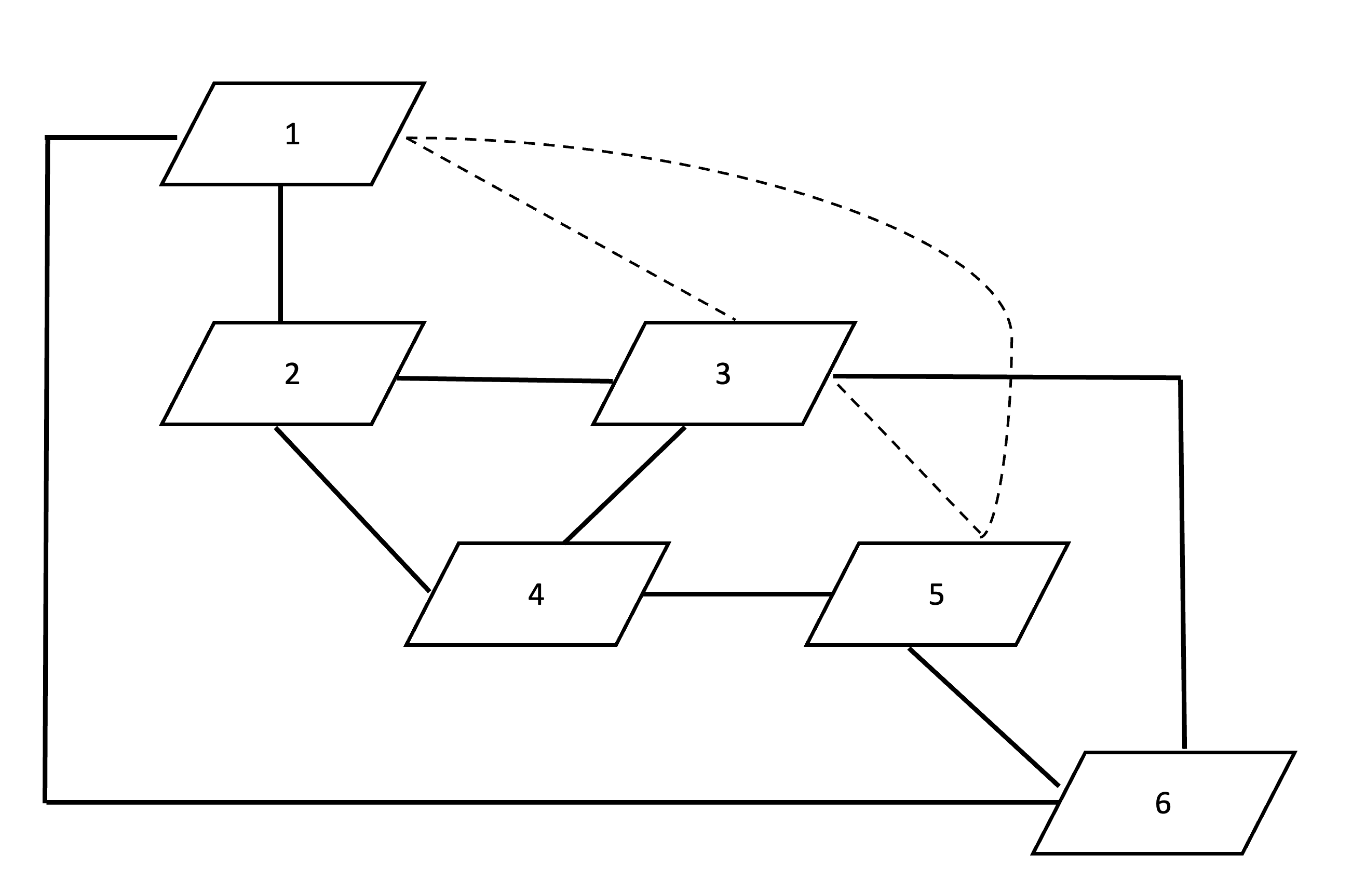
(b) Moralised structure

Figure 12: Schematic representations of the structure of six fields. The left figure is the original graph structure as in Figure 6, while the right figure displays the corresponding moralised structure. The dotted lines indicate the moralisation, or “marriage”, of parent fields that share a common child field.

After the moralisation, field “1” will be conditionally independent of field “4”; field “2” will be conditionally independent of fields “5” and “6”; field “4” will be conditionally independent of fields “1” and “6”; field “5” will be conditionally independent of field “2”; and field “6” will be conditionally independent of fields “2”, “4”.

The table 6 below shows the one-fold cross-validation results for the denoising and gap-filling for the 50 testing locations under two different b functions. The metrics used for cross-validation are mean absolute error (MAE) and root-mean-square error (RMSE).

Table 6: One-fold Cross-validation Results for Denoising and Gap-filling using the Mixed Conditional

	MAE	RMSE
Tri-Wave	1.1056	1.3806
Wendland	1.0027	1.2196

10.2 2D 5-fields: CAMS reanalysis data

For 2D illustration, we use CAMS reanalysis data introduced in Section 1. The graph structure follows the scientific evidence stated in Section 1 and is organised in Figure 13(a). The corresponding moralised graph is in Figure 13(b).

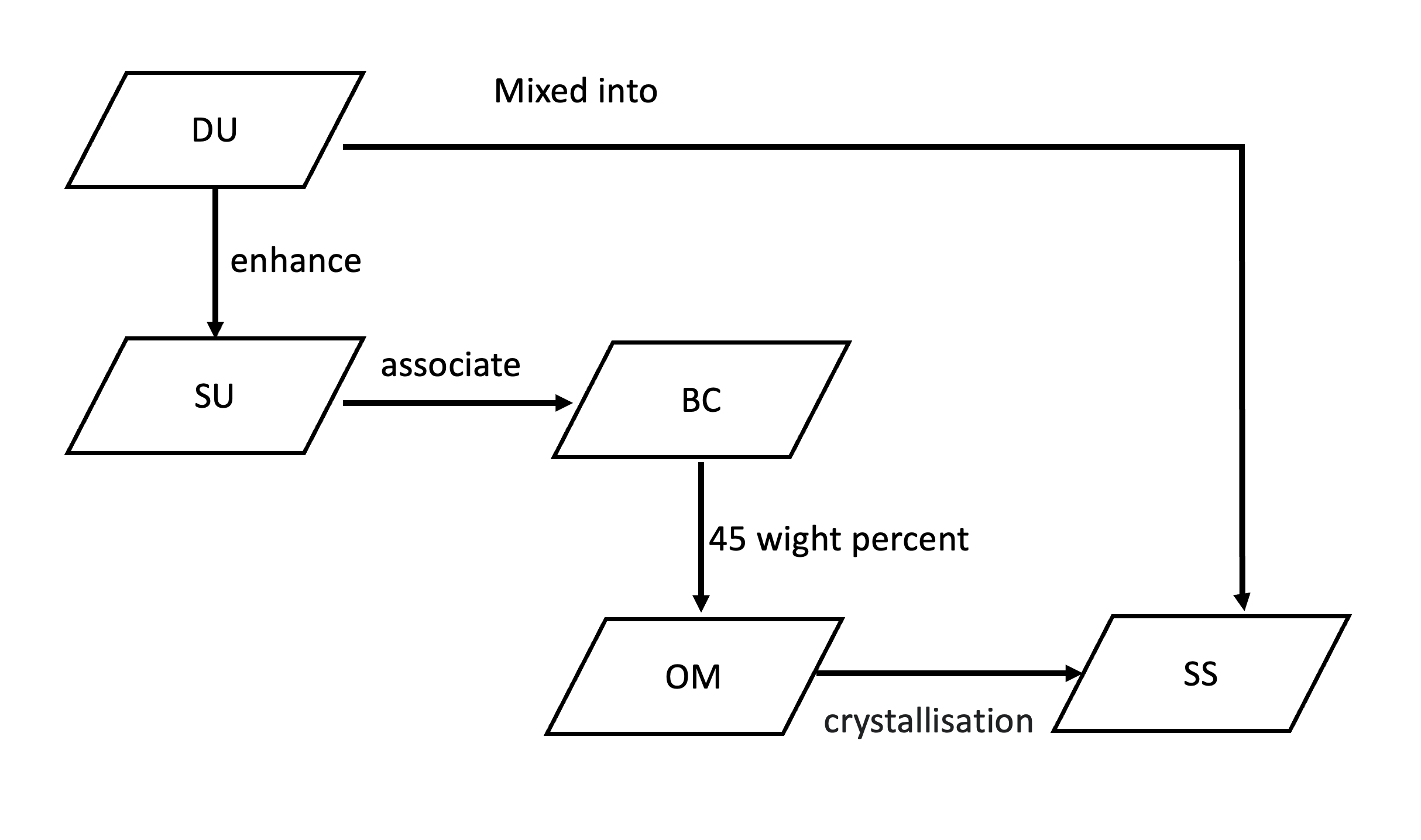
(a) Original structure

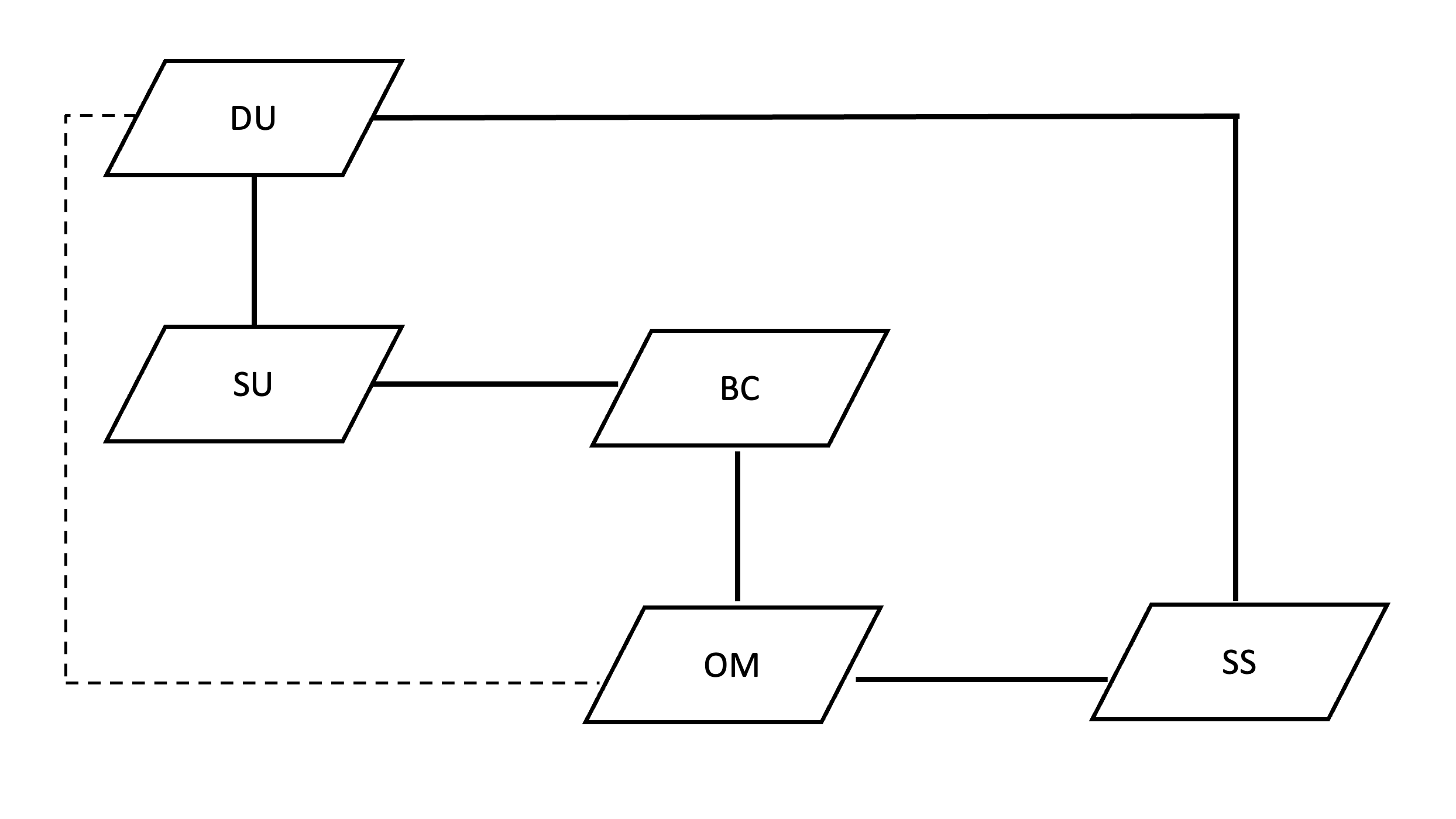
(b) Moralised structure

Figure 13: Schematic representations of the structure of CAMS reanalysis data. The left figure is the original graph structure organised according to scientific evidence, while the right figure displays the corresponding moralised structure. The dotted lines indicate the moralisation, or “marriage”, of parent fields that share a common child field.

As mentioned in Section 1, the CAMS is highly multivariate and high spatial dimensionality (spatial locations n = 27384), so the covariance and precision matrix to be constructed is of size $(27384*5)\times(27384*5)$ and is around 139.68 GB in memory. Since the largest memory of a single GPU node (NVIDIA A100 GPUs) available on Baskerville HPC is 80 GB, it is inevitable that the whole domain is segmented into smaller sections.

We divide the whole domain into four equal widths of longitude strips, as seen in Section 1, resulting in the first longitude strip (Lon-Strip-1) having 3793 spatial locations, the second (Lon-Strip-2) having 6581 spatial grids, the third having 10155 spatial locations, and the last (Lon-Strip-4) has 6855 spatial locations.

To fully utilise the HPC resource, large matrix multiplications in steps 24-30 in Algorithm 2 are offloaded to GPU for the construction of $\scalebox{1.5}{$\Sigma$}^{-1}_{np\times np}$, while the construction of $\scalebox{1.5}{$\Sigma$}_{np\times np}$ in steps 5-23 in Algorithm 2 remains in the CPU. This is because the latter involves nested for loops, which will force the code to be offloaded to the GPU and then sent back to the CPU at each iteration of the loop, implying very large communication overheads and low efficiency ultimately.

In practice, the GPU offloading is implemented through the R [27] package torch [12], a deep learning framework that utilises tensor and neural networks with GPU acceleration, and the package GPUmatrix [22].

Table 7 provides the time of one complete construction of $\scalebox{1.5}{$\Sigma$}_{np\times np}$ (on the CPU) and $\scalebox{1.5}{$\Sigma$}^{-1}_{np\times np}$ (offloaded to the GPU) for the data in the first Lon-Strip-1, consisting of 3793 spatial locations and 5 variate fields. The memory size of the corresponding covariance and precision matrix is around 2.7 GB. The table also displaces the time of one complete construction of $\scalebox{1.5}{$\Sigma$}_{np\times np}$ and $\scalebox{1.5}{$\Sigma$}^{-1}_{np\times np}$ done on a solo CPU. It shows that the construction time of the computing strategy with GPU offloading is more than five times faster than the strategy on the CPU only.

Table 7: Time for One Complete Construction of Joint Var-covariance Matrix and Precision Matrix with Two Computing Strategies: CPU + GPU vs. Solo CPU.

Construction computing strategy	Time
$\scalebox{1.5}{$\Sigma$}_{np\times np}$ (CPU) + $\scalebox{1.5}{$\Sigma$}^{-1}_{np\times np}$ (GPU)	01:27:49
$\scalebox{1.5}{$\Sigma$}_{np\times np}$ and $\scalebox{1.5}{$\Sigma$}^{-1}_{np\times np}$ (solo CPU)	05:18:52

Such a one complete $\scalebox{1.5}{$\Sigma$}_{np\times np}$ and $\scalebox{1.5}{$\Sigma$}^{-1}_{np\times np}$ construction time is roughly the time for one step out of multiple steps of one iteration of traditional L-BFGS-B optimisation. On average, one complete iteration of L-BFGS-B optimisation would require five line search steps; therefore, five complete constructions of $\scalebox{1.5}{$\Sigma$}_{np\times np}$ and $\scalebox{1.5}{$\Sigma$}^{-1}_{np\times np}$ in one iteration. This means to finish one complete iteration of traditional optimisation, one would need at least 450 minutes (5 * 90 mins) by Table 7. And to achieve convergence, it usually takes 150-200 such iterations, that is 450 * 150 = 67500 minutes = 1125 hours = 46.875 days.

However, the longest wall time allowed for a single job on Baskerville HPC is only ten days. This means that even with the construction of $\scalebox{1.5}{$\Sigma$}^{-1}_{np\times np}$ offloaded to the GPU, it is still not possible to finish the inference task using the traditional optimisation method.

Therefore, given the results in both Table 7 and the constraints of the Baskerville HPC resource (i.e., ten days wall time and 80 GB per GPU node), we conclude that a better inference method, in terms of faster convergence speed even under a large parameter space and more economical GPU memory storage, remains a missing piece of the HMHD spatial puzzle. We defer further discussions to Section 11.

11 Discussion

Highly multivariate high-dimensionality (HMHD) spatial statistics is a frontier topic. The data set involved in this topic features not only highly multivariate but also large spatial dimensionality.

This paper proposed a method for constructing the desired joint covariance $\scalebox{1.5}{$\Sigma$}_{np\times np}$ and precision matrix $\scalebox{1.5}{$\Sigma$}_{np\times np}^{-1}$ for the class of HMHD spatial data. To our knowledge, the proposed method is the first to comprehensively address all aspects of features of this class of data in the current literature.

Specifically, we defined a mixed spatial graph (see Section 3) and a mixed spatial graphical model framework (see Section 4). The first-stage model can account for the CI among $p$ ($p\gg 2$) variate fields for any customised graph relationship, including a special instance fully connected graph. The Algorithm 1 generates the desired $\scalebox{1.5}{$\Sigma$}_{np\times np}$ and $\scalebox{1.5}{$\Sigma$}_{np\times np}^{-1}$ in parallel, with the $\scalebox{1.5}{$\Sigma$}_{np\times np}^{-1}$’s generation order scales only linearly in $p$. This alleviates the $\scalebox{1.5}{$\Sigma$}_{np\times np}^{-1}$ generation burden dramatically compared with Cholesky inversion having a $\mathcal{O}(n^{3}p^{3})$ computational order and is therefore exorbitantly expensive in an HMHD spatial setting where both $p$ and $n$ are large.

The second-stage model further expands the CI from among $p$ variates to $n$ spatial locations. To achieve this, we showed the multivariate Hammersley-Clifford theorem from a column-wise conditional perspective, innovated new concepts such as cross-neighbourhood, and unearthed the existence of cross-MRF and its conditions (see Section 6). The link between the mixed spatial graphical model framework and the cross-MRF eventually enabled the desired CI among both $p$ and $n$, forming a mixed conditional modelling approach (see Section 7).

Such a mixed conditional approach provided the sparsest possible representations of $\scalebox{1.5}{$\Sigma$}_{np\times np}^{-1}$, with the highest possible exact-zero-value percentage, alongside the lowest possible $\scalebox{1.5}{$\Sigma$}_{np\times np}^{-1}$ generation order and fastest possible generation speed (see the various comparison tables in Section 7.3). Such results would consequently benefit the following inference for the HMHD spatial data.

The mixed conditional approach offers genuine advances over the current literature that deals with the conditional modelling approach. It overcomes the shortcomings in row-wise conditional [24] that only considered the CI among $n$ spatial locations; instead, it allows the joint accounting for the CI among both $p$ variates and $n$ spatial locations. The parallel construction of $\scalebox{1.5}{$\Sigma$}_{np\times np}$ and $\scalebox{1.5}{$\Sigma$}_{np\times np}^{-1}$ enables the incorporation of asymmetric cross-covariance blocks in the joint $\scalebox{1.5}{$\Sigma$}_{np\times np}$.

The mixed conditional also addresses the multiple deficiencies in the col-wise conditional [8] that only emphasised the asymmetric cross-covariance blocks in $\scalebox{1.5}{$\Sigma$}_{np\times np}$, neglected the CI in both $p$ and $n$ and obtained the desired $\scalebox{1.5}{$\Sigma$}_{np\times np}^{-1}$ at an extremely expensive cost via a further Cholesky inversion step from the giant $\scalebox{1.5}{$\Sigma$}_{np\times np}$. The algorithm associated with the mixed conditional enables one to obtain the desired $\scalebox{1.5}{$\Sigma$}_{np\times np}^{-1}$ on the fly and at computational cost only $\mathcal{O}(pn^{2})$; see the comparison Table 11 in Section 9.

Section 6.3 defines the cross-MRF, requiring the conditionally dependent variates $k$ and $l$ to be symmetric, and meanwhile, $s_{j}\in\mathcal{N}(s_{i})$. In the context of the mixed spatial graphical model framework, these conditions boil down to the constraint only on the variate fields modelled using DAG must be moralised (see section 7.1). This constraint, uncovered during the exploration of the doubly CI within the mixed spatial graphical model framework in the second-stage model, was actually hidden in the first-stage model.

As a result of moralisation, parent fields sharing a common child field are connected by undirected edges, while arrows on the other directed edges are removed, transforming the structure into an undirected graph.

This transformation clarifies the discrepancy between the CI among $p$ variate fields embedded in the DAG for cross-variate fields and the sparse structure observed in the joint precision matrix plots (see Figure 7 and Figure 8), as described in Observation 2 in the first-stage model. More concretely, after moralisation, field “5” and fields “1”, “3”, “4”, and “6” are in one clique. No differentiation of auto- or cross-clique is made here since $s_{j}\in\mathcal{N}(s_{i})$ is not yet considered as part of the first-stage model. As a result, field “5” is conditionally independent of field “2” only. Thus, Observation 2 is explained.

We notice a consistent relationship between the sparsity in the inverse of univariate covariance matrices, e.g., $\Sigma_{11}^{-1}$, and that in the $\scalebox{1.5}{$\Sigma$}^{-1}_{np\times np}$, meaning the sparser the inverse of univariate covariance matrices, the sparser the $\scalebox{1.5}{$\Sigma$}_{np\times np}^{-1}$. This suggests that our strategy using univariate CAR in Section 7.2 to realise the $s_{j}\in\mathcal{N}(s_{i})$ for linking the cross-MRF and the mixed spatial graphical model and to eventually realise the desired mixed conditional is efficacious.

Such a co-existence between univariate CAR (equivalently univariate MRF) and joint $\scalebox{1.5}{$\Sigma$}^{-1}_{np\times np}$ and $\scalebox{1.5}{$\Sigma$}_{np\times np}$ for geostatistical processes in one unified framework provides a potential solution to an open problem; See Section 8.

We also find a natural fit between our proposed algorithms and the HPC resource, particularly in the construction of the $\scalebox{1.5}{$\Sigma$}^{-1}_{np\times np}$. With the large matrix multiplications being offloaded to GPUs, the proposed solution to fully address all facets of features of the HMHD spatial data is propelled to even greater acceleration.

From the results in Section 10.2, we realise that the traditional optimisation inference methods are not sufficient enough for the HMHD spatial problem, and we recognise that a better inference method that could offer speedy convergence and affordable memory storage is still a missing piece of the HMHD spatial puzzle.

We did not embark on the traditional Bayesian inference method either because, in an HMHD spatial setting, there are usually numerous parameters. So, non-parametric Bayesian and/or variational Bayesian inference might be future work.

12 Acknowledgements

The first author is supported by The Alan Turing Institute doctoral scholarship. This research was supported in part through computational resources provided by The Alan Turing Institute under EPSRC grant EP/N510129/1. The computations described in this research were performed using the Baskerville Tier 2 HPC service (https://www.baskerville.ac.uk/). Baskerville was funded by the EPSRC and UKRI through the World Class Labs scheme (EP/T022221/1) and the Digital Research Infrastructure programme (EP/W032244/1). The data is downloaded from the Copernicus Atmosphere Monitoring Service (CAMS) Atmosphere Data Store (ADS) (https://ads.atmosphere.copernicus.eu/cdsapp#!/dataset/cams-global-reanalysis-eac4?tab=overview).

Appendix A Proof of Lemma 2

Proof.

Re-arrange equation (5), we have

$$(\bm{I}-\mathcal{B})(\bm{Y}-\bm{\mu})=\bm{S}\bm{Z},$$ (51)

by Lemma 1, we know $(\bm{I}-\mathcal{B})$ is non-sigular, as the diagonal elements of $\mathcal{B}$ is $\{b_{ll}(s_{i},s_{i}):i=1,2,\ldots,n;l=1,2,\ldots,p\}$, so we have

$$\bm{Y}=\bm{\mu}+(\bm{I}-\mathcal{B})^{-1}\bm{S}\bm{Z},$$

therefore, we arrive

$$\scalebox{1.5}{$\Sigma$}_{np\times np}=Var[\bm{Y}]=(\bm{I}-\mathcal{B})^{-1}\bm{D}(\bm{I}-\mathcal{B})^{-T},$$ (52)

where $\bm{S}=\bm{D}^{\frac{1}{2}}$. ∎

Appendix B Proof of Theorem 1

When $k=\{1,2,\ldots,r\}$, $l=\{(r+1),\ldots,p\}$, [29, Appendix. B, Theorem 7 ] states a general form for non-spatial multivariate multiple regression, as below

$$\bm{Y}_{l}=\bm{\mu}_{l}+\bm{U}_{lk}\bm{E}_{k}+\bm{U}_{ll}\bm{E}_{l},$$ (53)

in which $\bm{U}_{lk}\triangleq(\bm{I}-\bm{B})^{-1}$, $\bm{E}\triangleq\bm{S}\bm{Z}$, $\bm{S}=\bm{D}^{1/2}$.

B.1 Lemma 5

Lemma 5.

When $l=\{p\},k=\{1,\cdots,(p-1)\}$, $\bm{U}_{lk}\bm{U}_{kk}^{-1}=\bm{B}_{lk}$.

Proof.

Without loss of generality, we set $P=5$ and assume a directed chain structure among p variates. $\bm{B}=[b_{lk}]$, where $b_{lk}=0$ if $k\notin Pa(l)$, and $b_{ll}=0$ as there’s no self-node regression.

So, $\bm{B}$ is $\left[\begin{array}[]{ccccc}0&&&&\\ b_{21}&0&&&\\ &b_{32}&0&&\\ &&b_{43}&0&\\ &&&b_{54}&0\end{array}\right],$ then $(\bm{I}-\bm{B})$ is $\left[\begin{array}[]{ccccc}1&&&&\\ -b_{21}&1&&&\\ &-b_{32}&1&&\\ &&-b_{43}&1&\\ &&&-b_{54}&1\end{array}\right],$ and by the formula of the inverse of the lower bi-diagonal matrix given in [18],

$(\bm{I}-\bm{B})^{-1}\triangleq\bm{U}=\left[\begin{array}[]{ccccc}1&&&&\\ b_{21}&1&&&\\ b_{32}b_{21}&b_{32}&1&&\\ b_{43}b_{32}b_{21}&b_{43}b_{32}&b_{43}&1&\\ b_{54}b_{43}b_{32}b_{21}&b_{54}b_{43}b_{32}&b_{54}b_{43}&b_{54}&1\end{array}\right].$

$\bm{U}_{lk}=\bm{U}_{\{5\}\{1,2,3,4\}}\left[\begin{array}[]{cccc}b_{54}b_{43}b_{32}b_{21}&b_{54}b_{43}b_{32}&b_{54}b_{43}&b_{54}\end{array}\right]$

$\bm{U}_{kk}^{-1}=\bm{U}_{\{1,2,3,4\}\{1,2,3,4\}}^{-1}=\left[\begin{array}[]{cccc}1&&&\\ -b_{21}&1&&\\ &-b_{32}&1&\\ &&-b_{43}&1\\ \end{array}\right],$ therefore, $\bm{U}_{lk}\bm{U}_{kk}^{-1}=\left[\begin{array}[]{cccc}0&0&0&b_{54}\end{array}\right]=\bm{B}_{\{5\}\{1,2,3,4\}}=\bm{B}_{lk}$, which is right the 5th row and the first four columns of matrix $\bm{B}$. ∎

B.2 Lemma 6

Lemma 6.

$$\bm{Y}_{l}=\bm{\mu}_{l}+\bm{U}_{lk}\bm{E}_{k}+\bm{U}_{ll}\bm{E}_{l},$$ (54)

is the general multivariate multiple regression form of

$$\bm{Y}_{l}=\bm{\mu}_{l}+\bm{B}_{lk}(\bm{Y}_{k}-\bm{\mu}_{k})+\bm{E}_{l}$$ (55)

Proof.

We know $\bm{S}\bm{Z}\triangleq\bm{E}=(\bm{I}-\bm{B})(\bm{Y}-\bm{\mu})$, so,

$$\bm{E}_{k} =\bm{U}_{kk}^{-1}(\bm{Y}_{k}-\bm{\mu}_{k})$$ (56)

$$\bm{U}_{lk}\bm{E}_{k} =\bm{U}_{lk}\bm{U}_{kk}^{-1}(\bm{Y}_{k}-\bm{\mu}_{k}),$$ (57)

and $\bm{U}_{ll}=(\bm{I}-\bm{B})_{ll}^{-1}=1$.

So, re-write equation (54) as

$$\bm{Y}_{l}=\bm{\mu}_{l}+\bm{U}_{lk}\bm{U}_{kk}^{-1}(\bm{Y}_{k}-\bm{\mu}_{k})+\bm{E}_{l}$$ (58)

By Lemma 5, when $l=\{p\}$, $k=\{1,2,\ldots,(p-1)\}$, equation (58) degenerates to one variate (outcome) multiple regression equation:

$$Y_{l}=\mu_{l}+\bm{B}_{lk}(\bm{Y}_{k}-\bm{\mu}_{k})+E_{l}$$

∎

B.3 Proof of Theorem 1

Proof.

We start from the general equation (54) and expand it to a spatial setting.

Let the variates $N=\{1,2,\ldots,p\}$, and divide it into two parts, one is $k=\{1,2,\ldots,r\}$, and the other is $l=\{(r+1),\ldots,p\}$

For any given location $s$, we have

$$\bm{Y}_{l}(s)=\bm{\mu}_{l}(s)+\int_{D}\bm{U}_{lk}(s,v)\bm{U}^{-1}_{kk}(v,v)[\bm{Y}_{k}(v)-\bm{\mu}_{k}(v)]dv+\bm{U}_{ll}(s,s)\bm{E}_{l}(s)$$

The covariance between a pair of locations $s_{i}$ and $s_{j}$ across all variates is

$$\scalebox{1.5}{$\Sigma$}(s_{i},s_{j}) =cov(\bm{Y}_{\cdot}(s_{i}),\bm{Y}_{\cdot}(s_{j}))$$

$$=\mathbb{E}\left[Var\left[\begin{array}[]{cc}\bm{Y}_{k}(s_{i})|\bm{Y}_{k}(\cdot)\\ \bm{Y}_{l}(s_{j})|\bm{Y}_{k}(\cdot)\end{array}\right]\right]+Var\left[\mathbb{E}\left[\begin{array}[]{cc}\bm{Y}_{k}(s_{i})|\bm{Y}_{k}(\cdot)\\ \bm{Y}_{l}(s_{j})|\bm{Y}_{k}(\cdot)\end{array}\right]\right]$$

in which,

$$\mathbb{E}\left[Var\left[\begin{array}[]{cc}\bm{Y}_{k}(s_{i})|\bm{Y}_{k}(\cdot)\\ \bm{Y}_{l}(s_{j})|\bm{Y}_{k}(\cdot)\end{array}\right]\right]$$

$$=\left[\begin{array}[]{cc}\bm{0}&\bm{0}\\ \bm{0}&cov[(\bm{Y}_{l}(s_{j}),\bm{Y}_{l}(s_{i})|\bm{Y}_{k}(\cdot))]\end{array}\right]$$

$$=\left[\begin{array}[]{cc}\bm{0}&\bm{0}\\ \bm{0}&cov[\bm{U}_{ll}(s_{j},s_{j})\bm{E}_{l}(s_{j}),\bm{U}_{ll}(s_{i},s_{i})\bm{E}_{l}(s_{i})]\end{array}\right]$$

$$=\left[\begin{array}[]{cc}\bm{0}&\bm{0}\\ \bm{0}&\bm{U}_{ll}(s_{j},s_{j})\bm{D}_{ll}(s_{j},s_{i})\bm{U}_{ll}^{T}(s_{i},s_{i})\end{array}\right]$$

$$\mbox{(by $\bm{E}_{l}(s_{i})$ $\triangleq$ $\bm{S}_{ll}(s_{i},s_{i})\bm{Z}_{l}(s_{i})$ )},$$

and

$$\mathbb{E}\left[\begin{array}[]{c}\bm{Y}_{k}(s_{i})|\bm{Y}_{k}(\cdot)\\ \bm{Y}_{l}(s_{j})|\bm{Y}_{k}(\cdot)\end{array}\right] =\mathbb{E}\left[\begin{array}[]{c}\bm{Y}_{k}(s_{i})\\ \mathbb{E}[\bm{Y}_{l}(s_{j})|\bm{Y}_{k}(\cdot)]\end{array}\right]$$

$$=\left[\begin{array}[]{c}\bm{Y}_{k}(s_{i})\\ \int_{D}\bm{U}_{lk}(s_{j},v)\bm{U}_{kk}^{-1}\bm{Y}_{k}(v)dv\end{array}\right]$$

$Var\left[\begin{array}[]{c}\bm{Y}_{k}(s_{i})\\ \int_{D}\bm{U}_{lk}(s_{j},v)\bm{U}_{kk}^{-1}\bm{Y}_{k}(v)dv\end{array}\right]=$

$$\left[\begin{array}[]{cc}\bm{\Sigma}_{kk}(s_{i},s_{j})&\int_{D}\bm{\Sigma}_{kk}(s_{i},v)(\bm{U}_{lk}(s_{j},v)\bm{U}_{kk}^{-1}(v,v))^{T}dv\\ \int_{D}\bm{U}_{lk}(s_{j},v)\bm{U}_{kk}^{-1}(v,v)\bm{\Sigma}_{kk}(v,s_{i})dv&\int\int\bm{U}_{lk}(s_{j},v)\bm{U}_{kk}^{-1}(v,v)\bm{\Sigma}_{kk}(v,w)(\bm{U}_{lk}(s_{i},w)\bm{U}_{kk}^{-1}(w,w))^{T}dvdw\end{array}\right],$$

When $l=\{p\}$, $k=\{1,2,\ldots,(p-1)\}$, $k\in Pa(l)$, by Lemma 5

$$\bm{U}_{lk}(s_{j},v)\bm{U}_{kk}^{-1}(v,v) =block[b_{lk}(s_{j},v)]\triangleq\bm{B}_{lk}(s_{j},v)$$

$$\bm{U}_{lk}(s_{i},w)\bm{U}_{kk}^{-1}(w,w) =block[b_{lk}(s_{i},v)]\triangleq\bm{B}_{lk}(s_{i},w)$$

So,

$$\scalebox{1.5}{$\Sigma$}(s_{i},s_{j}) =\left[\begin{array}[]{cc}\bm{\Sigma}_{kk}(s_{i},s_{j})&\int\bm{\Sigma}_{kk}(s_{i},v)\bm{B}_{lk}^{T}(s_{j},v)dv\\ \int\bm{B}_{lk}(s_{j},v)\bm{\Sigma}_{kk}(v,s_{i})dv&\int\int\bm{B}_{lk}\bm{\Sigma}_{kk}(v,w)\bm{B}_{lk}^{T}(s_{i},w)dvdw+\bm{D}_{ll}(s_{j},s_{i})\end{array}\right]$$

From one pair of location $(s_{i},s_{j})$ to all locations $[s_{1},\ldots,s_{n}]^{\prime}$, we get

$$\scalebox{1.5}{$\Sigma$}=\left[\begin{array}[]{cc}\bm{\Sigma}_{kk}(\cdot,\cdot)&\bm{\Sigma}_{kk}(\cdot,\cdot)\bm{B}^{T}_{lk}(\cdot,\cdot)\\ \bm{B}_{lk}(\cdot,\cdot)\bm{\Sigma}_{kk}(\cdot,\cdot)&\bm{B}_{lk}(\cdot,\cdot)\bm{\Sigma}_{kk}(\cdot,\cdot)\bm{B}_{lk}^{T}(\cdot,\cdot)+\bm{D}_{ll}(\cdot,\cdot)\end{array}\right]$$

As matrix multiplication automatically sums over all process locations $v^{\prime}s$ and $w^{\prime}s$, $\Sigma$ is free of integration.

To obtain the induction formula, let $l=\{j+1\}$, $k=\{1,2,\ldots,j:k\in Pa(l)\}$,

$$\scalebox{1.5}{$\Sigma$}=\left[\begin{array}[]{cc}\bm{\Sigma}_{\{1,\ldots,j\}\{1,\ldots,j\}}(\cdot,\cdot)&\bm{\Sigma}_{\{1,\ldots,j\}\{1,\ldots,j\}}(\cdot,\cdot)\bm{B}_{\{j+1\}\{1,\ldots,j\}}^{T}(\cdot,\cdot)\\ \bm{B}_{\{j+1\}\{1,\ldots,j\}}\bm{\Sigma}_{\{1,\ldots,j\}\{1,\ldots,j\}}(\cdot,\cdot)&\bm{B}_{\{j+1\}\{1,\ldots,j\}}\bm{\Sigma}_{\{1,\ldots,j\}\{1,\ldots,j\}}\bm{B}_{\{j+1\}\{1,\ldots,j\}}^{T}+\bm{D}_{\{j+1\}\{j+1\}}(\cdot,\cdot)\end{array}\right]$$

∎

Appendix C Trivariate Process SIGMA

$$\scalebox{1.5}{$\Sigma$}_{3n\times 3n}$$

$$=\left[\begin{array}[]{cc}\bm{\Sigma}_{\{1,2\}\{1,2\}}(\cdot,\cdot)&\bm{\Sigma}_{\{1,2\}\{1,2\}}(\cdot,\cdot)\bm{B}_{\{3\}\{1,2\}}^{T}(\cdot,\cdot)\\ \bm{B}_{\{3\}\{1,2\}}(\cdot,\cdot)\bm{\Sigma}_{\{1,2\}\{1,2\}}(\cdot,\cdot)&\bm{B}_{\{3\}\{1,2\}}\bm{\Sigma}_{\{1,2\}\{1,2\}}\bm{B}_{\{3\}\{1,2\}}^{T}+\bm{D}_{\{3\}\{3\}}(\cdot,\cdot)\end{array}\right]$$

$$=\left[\begin{array}[]{cc}\left[\begin{array}[]{cc}\bm{\Sigma}_{11}&\bm{\Sigma}_{12}\\ \bm{\Sigma}_{21}&\bm{\Sigma}_{22}\end{array}\right]&\left[\begin{array}[]{cc}\bm{\Sigma}_{11}&\bm{\Sigma}_{12}\\ \bm{\Sigma}_{21}&\bm{\Sigma}_{22}\end{array}\right]\left[\begin{array}[]{c}\bm{B}_{31}^{T}\\ \bm{B}_{32}^{T}\end{array}\right]\\ \left[\begin{array}[]{cc}\bm{B}_{31}\bm{B}_{32}\end{array}\right]\left[\begin{array}[]{cc}\bm{\Sigma}_{11}&\bm{\Sigma}_{12}\\ \bm{\Sigma}_{21}&\bm{\Sigma}_{22}\end{array}\right]&\left[\begin{array}[]{cc}\bm{B}_{31}\bm{B}_{32}\end{array}\right]\left[\begin{array}[]{cc}\bm{\Sigma}_{11}&\bm{\Sigma}_{12}\\ \bm{\Sigma}_{21}&\bm{\Sigma}_{22}\end{array}\right]\left[\begin{array}[]{c}\bm{B}_{31}^{T}\\ \bm{B}_{32}^{T}\end{array}\right]+\bm{D}_{33}\end{array}\right]$$

if 1 $$\in Pa(3)$$

$$=\left[\begin{array}[]{ccc}\bm{\Sigma}_{11}&\bm{\Sigma}_{12}&\bm{\Sigma}_{11}\bm{B}_{31}^{T}\\ \bm{\Sigma}_{21}&\bm{\Sigma}_{22}&\bm{\Sigma}_{21}\bm{B}_{31}^{T}\\ \bm{B}_{31}\bm{\Sigma}_{11}&\bm{B}_{31}\bm{\Sigma}_{12}&\bm{\Sigma}_{31}\bm{B}_{31}^{T}+\bm{D}_{33}\end{array}\right]$$

if 2 $$\in Pa(3)$$

$$=\left[\begin{array}[]{ccc}\bm{\Sigma}_{11}&\bm{\Sigma}_{12}&\bm{\Sigma}_{12}\bm{B}_{32}^{T}\\ \bm{\Sigma}_{21}&\bm{\Sigma}_{22}&\bm{\Sigma}_{22}\bm{B}_{32}^{T}\\ \bm{B}_{32}\bm{\Sigma}_{21}&\bm{B}_{32}\bm{\Sigma}_{22}&\bm{\Sigma}_{32}\bm{B}_{32}^{T}+\bm{D}_{33}\end{array}\right]$$

if 1, 2 $$\in Pa(3)$$

$$=\left[\begin{array}[]{ccc}\bm{\Sigma}_{11}&\bm{\Sigma}_{12}&\bm{\Sigma}_{11}\bm{B}_{31}^{T}+\bm{\Sigma}_{12}\bm{B}_{32}^{T}\\ \bm{\Sigma}_{21}&\bm{\Sigma}_{22}&\bm{\Sigma}_{21}\bm{B}_{31}^{T}+\bm{\Sigma}_{22}\bm{B}_{32}^{T}\\ \bm{B}_{31}\bm{\Sigma}_{11}+\bm{B}_{32}\bm{\Sigma}_{21}&\bm{B}_{31}\bm{\Sigma}_{12}+\bm{B}_{32}\bm{\Sigma}_{22}&\bm{\Sigma}_{31}\bm{B}_{31}^{T}+\bm{\Sigma}_{32}\bm{B}_{32}^{T}+\bm{D}_{33}\end{array}\right]$$

Appendix D Algorithm 1

Data: The number of variates $p$ and the data structure indicating parent and child relationship among $p$ variates

Result: The desired $\scalebox{1.5}{$\Sigma$}_{np\times np}(\cdot,\cdot)$ and $\scalebox{1.5}{$\Sigma$}^{-1}_{np\times np}(\cdot,\cdot)$

1

2$\bm{\Sigma}_{11}\leftarrow$ known (e.g., exponential, Matérn) ;

3 $\scalebox{1.5}{$\Sigma$}\leftarrow\bm{\Sigma}_{11}$; $n\leftarrow nrow(\bm{\Sigma}_{11})$ ;

4

5for $r=2$ to $p$ do

6        PN = Pa(r) ;

7        $\bm{R}=\bm{C}=NULL$ ;

8        for $c=1$ to $(r-1)$ do

9               $\bm{BT}\leftarrow NULL$ ;

10               $\bm{\Sigma}_{rc}\leftarrow\bm{0}$;

11               for t $\in$ PN do

12                      $\bm{B}_{rt}\leftarrow f(h;\Delta_{rt};A_{rt})$ ;

13                      $\bm{BT}\leftarrow rbind(\bm{BT},\bm{B}_{rt}^{T})$;

14                      $\bm{\Sigma}_{rc}\leftarrow\bm{\Sigma}_{rc}+\bm{B}_{rt}\bm{\Sigma}[((t-1)n+1):(tn),((c-1)n+1):(cn)]$ ;

15                     

16              

17              $\bm{R}\leftarrow cbind(\bm{R},\bm{\Sigma}_{rc})$ ;

18               $\bm{\Sigma}_{cr}\leftarrow\bm{\Sigma}_{rc}^{T}$ ;

19               $\bm{C}\leftarrow rbind(\bm{C},\bm{\Sigma}_{cr})$ ;

20              

21       

22       $\bm{D}_{rr}\leftarrow$ known (e.g., exponential, Matérn) ;

23        $\bm{\Sigma}_{rr}\leftarrow\bm{R}[,(t-1)n+1:(tn)]\bm{BT}+\bm{D}_{rr}$ ;

24       

25       $SG\leftarrow\scalebox{1.5}{$\Sigma$}$

26       $Col\leftarrow rbind(\bm{C},\bm{\Sigma}_{rr})$ ;

27        $Row\leftarrow rbind(SG,\bm{R})$ ;

28        $\scalebox{1.5}{$\Sigma$}\leftarrow cbind(Row,Col)$ ;

29       

30       $\bm{D}_{rr}^{-1}\leftarrow$ Cholesky inversion ($\bm{D}_{rr}$);

31       

32       if  r== 2 then

33              SG${}^{-1}\leftarrow$ Cholesky inversion (SG)

34       $BK_{1}\leftarrow SG^{-1}[SG+\bm{C}\bm{D}_{rr}^{-1}\bm{R}]SG^{-1}$ ;

35        $BK_{2}\leftarrow-SG^{-1}\bm{C}\bm{D}_{rr}^{-1}$ ;

36        $BK_{3}\leftarrow-\bm{D}_{rr}^{-1}\bm{R}SG^{-1}$ ;

37        $BK_{4}\leftarrow\bm{D}_{rr}^{-1}$ ;

38       

39       $\scalebox{1.5}{$\Sigma$}^{-1}\leftarrow rbind(cbind(BK1,BK2),cbind(BK3,BK4))$ ;

40        $SG^{-1}\leftarrow\scalebox{1.5}{$\Sigma$}^{-1}$

41       if r == p then

42              return

$\Sigma$

, $\scalebox{1.5}{$\Sigma$}^{-1}$

43       

Algorithm 1 Algorithm for the generation of the desired $\Sigma$ and $\Sigma^{-1}$

Appendix E Plots of Modified Tri-Wave

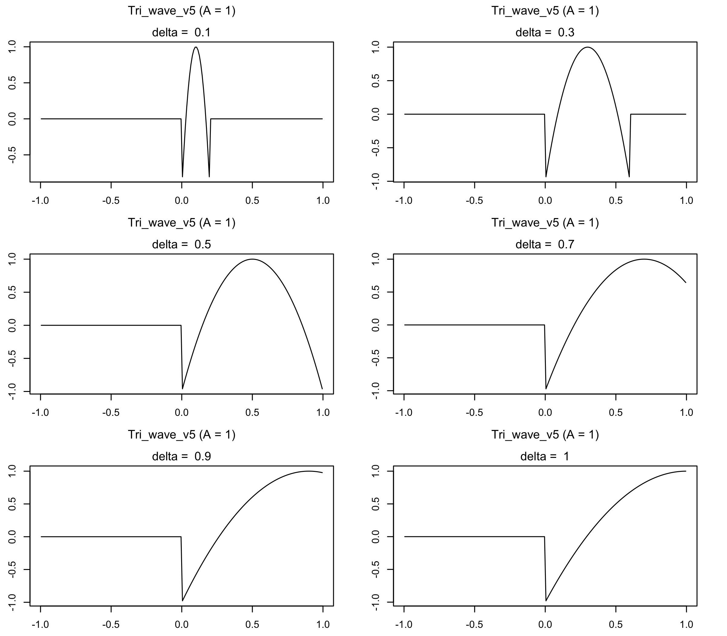
Figure 14: 1D plots of the modified Tri-Wave(h; $A=1$, $\Delta$) in which the manually-set factor $\phi=2$, $\rho=1$. $\Delta$s are all positive values.

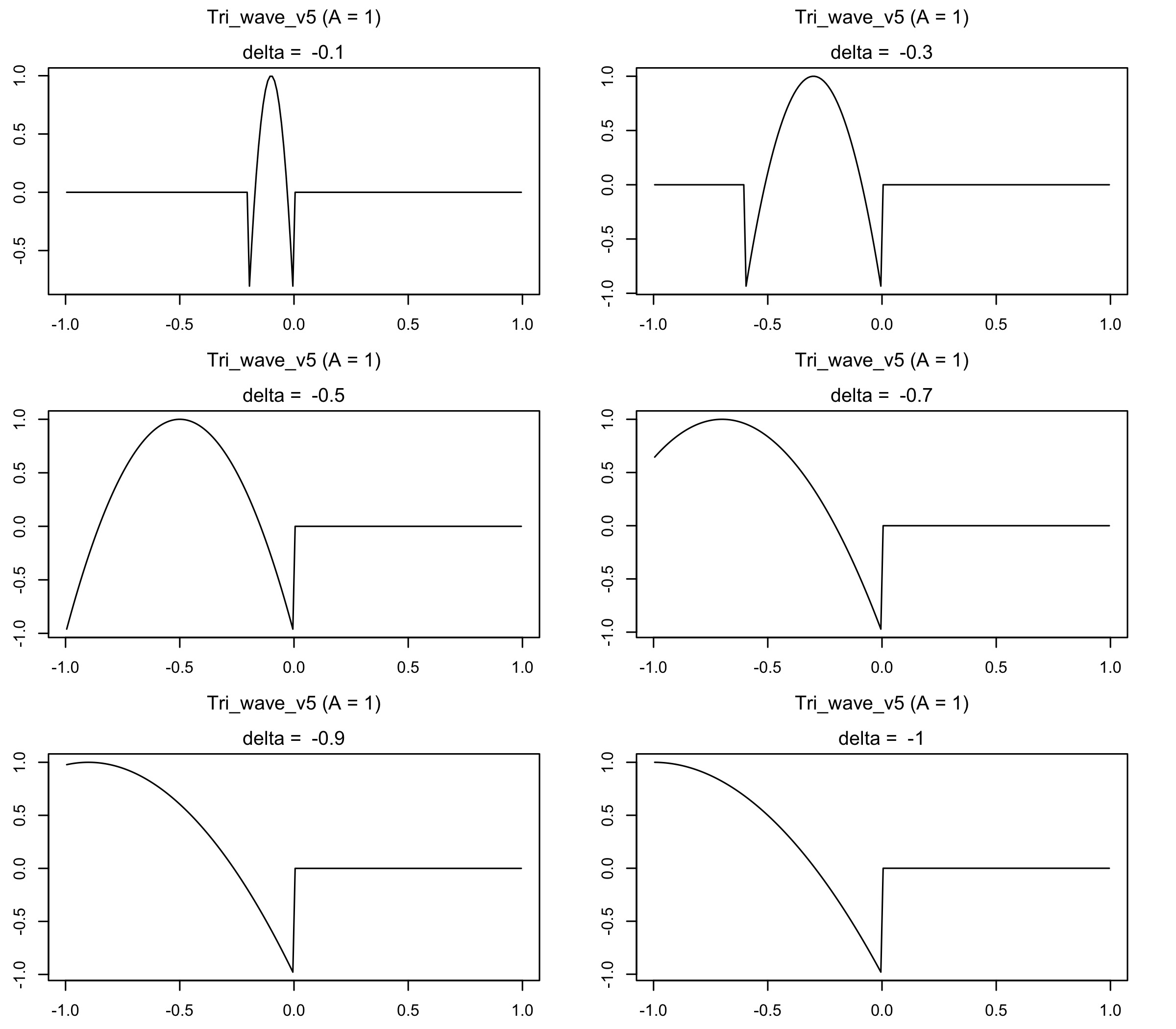
Figure 15: 1D plots of the modified Tri-Wave(h; $A=1$, $\Delta$) in which the manually-set factor $\phi=2$, $\rho=1$. $\Delta$s are all negative values.

Appendix F Wendland function

Wendland function [33]

$$Wendland_{k}(r)=\left\{\begin{array}[]{rcl}A\{1-(\frac{/r-\Delta/}{R})^{2k+1}(1+(2k+1)\frac{/r-\Delta/}{R})\}&\mbox{for}&/h-\Delta/\geq R\\ 0&\mbox{for}&/h-\Delta/>R\end{array}\right.,$$ (61)

in which $A$ (amplitude) and $\Delta$ (translation) are parameters obtained from inference, while $k$ and $R$ are manually set factors. $k$ controls the smoothness (continuously differentiability) of the function and is set to the same value as the smoothness $\nu$ in Matérn, e.g., 3/2 for special Matérn. $R$ is the compact support radius beyond which the function values are set to exact zero. If this Wendland function is used to model the covariance, it also embodies the meaning of effective range, at which the spatial correlation drops to a negligible 0.05, see [13]; For the shape of the Wendland function (k = 3/2), see below Figure 16.

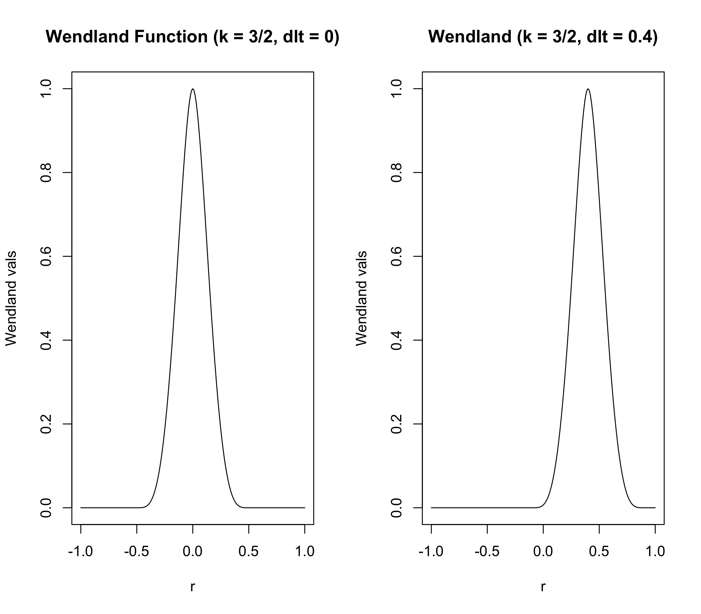
Figure 16: Wendland function where smoothness $k=3/2$. The spatial domain is a sequence from -1 to 1 by 0.01, and the $R$ is set to 0.5. The left figure corresponds to translation $\Delta=0$, and the right corresponds to $\Delta=0.4$.

Appendix G Test Report on the Robustness of the Positive Definiteness of $\Sigma$ and $\Sigma^{-1}$

The aim of this section is to test the robustness of the positive definiteness (PD) of $\Sigma$ and $\scalebox{1.5}{$\Sigma$}^{-1}$ constructed using Algorithm 1 with original $\bm{B}_{rt}$ ($\bm{B}_{rt}^{Original}$) functions and $\bm{B}_{rt}$ undergone spectral normalisation together with regularisation ($\bm{B}_{rt}^{SpN+Reg}$).

The test settings are three versions of the modified Tri-Wave functions and one version of the Wendland function (k = 3/2) for $\bm{B}_{rt}$ on three combinations of grid size (ds) and domain ($\mathcal{D}$), i.e., $\{ds=0.1,\mathcal{D}=[-1,1]\}$, $\{ds=0.05,\mathcal{D}=[-1,1]\}$, $\{ds=0.1,\mathcal{D}=[-10,10]\}$ under two graph structures corresponds to two fields (p = 5, p = 7), see Figure 17.

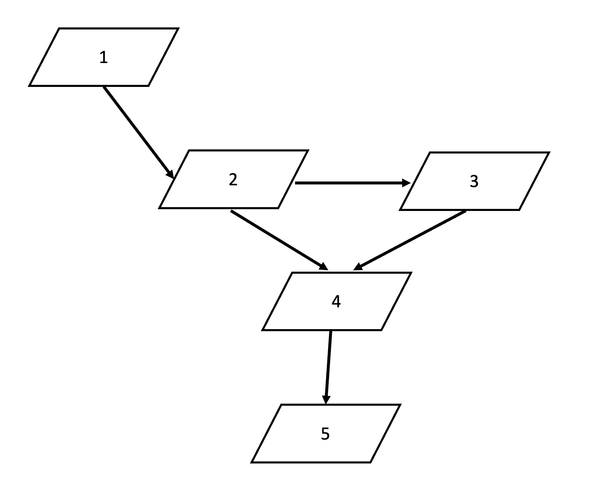
(a) A randomly drawn acyclic graph for five fields

(b) A randomly drawn acyclic graph for seven fields

Figure 17: Randomly drawn acyclic graphs for tests

The modified Tri-Wave function is

$$Tri-Wave(h)=\left\{\begin{array}[]{rcl}A\{1-\phi(\frac{/h-\Delta/}{/\Delta/})^{2}\}&\mbox{for}&/h-\Delta/\leq\rho/\Delta/\\ 0&\mbox{for}&/h-\Delta/>\rho/\Delta/\end{array}\right.$$

and the three versions are V4 ($\phi=1/2,\rho=2$), V5 ($\phi=2,\rho=1$), and V7 ($\phi=2,\rho=2$).

The Wendland function used in tests adopts $k=3/2$ and $R=0.5$, i.e.,

$$Wendland_{k}(r)=\left\{\begin{array}[]{rcl}A\{1-(\frac{/r-\Delta/}{R})^{4}(1+4\frac{/r-\Delta/}{R})\}&\mbox{for}&/h-\Delta/\leq R\\ 0&\mbox{for}&/h-\Delta/>R\end{array}\right.$$ (64)

The PD is tested using 100 parameter combinations, where $A$ ranges from 0.1 $\sim$ 1, and $\Delta$ ranges from 0.1 $\sim$ 1, both by 0.1.

The test results are presented below in Table 8 and 9.

Table 8: Test Report on the Positive Definiteness of $\Sigma$ and $\Sigma^{-1}$ using $\bm{B}_{rt}^{Original}$ and $\bm{B}_{rt}^{SpN+Reg}$ with Different Versions of Modified Tri-Wave

Version $(\phi$, $\rho)$	Grid size	Domain $\mathcal{D}$	Field No. p	$\bm{B}_{rt}^{Original}$	$\bm{B}_{rt}^{SpN+Reg}$
V4 (1/2, 2)	ds = 0.1	$[-1,1]$	7	few $\scalebox{1.5}{$\Sigma$}^{-1}$ PD	all $\scalebox{1.5}{$\Sigma$}^{-1}$, $\Sigma$ PD no perturb required
V4 (1/2, 2)	ds = 0.05	$[-1,1]$	7	6 $\Sigma$ not PD; none of $\scalebox{1.5}{$\Sigma$}^{-1}$ PD	all $\scalebox{1.5}{$\Sigma$}^{-1}$, $\Sigma$ PD no perturb required
V4 (1/2, 2)	ds = 0.1	$[-10,10]$	5	none of $\scalebox{1.5}{$\Sigma$}^{-1}$ PD	all $\scalebox{1.5}{$\Sigma$}^{-1}$, $\Sigma$ PD no perturb required
V4 (1/2, 2)	ds = 0.1	$[-10,10]$	7	none of $\scalebox{1.5}{$\Sigma$}^{-1}$ PD; few $\Sigma$ PD; only field 1-3 PD; field 4$\sim$7 all non-PD	20 $\scalebox{1.5}{$\Sigma$}^{-1}$ not PD; the rest require perturb 0.001 $\sim$ 0.2; $\Sigma$ , $\scalebox{1.5}{$\Sigma$}^{-1}$ PD in field 1$\sim$6
V5 (2, 1)	ds = 0.1	$[-1,1]$	7	none of $\scalebox{1.5}{$\Sigma$}^{-1}$ PD	all $\scalebox{1.5}{$\Sigma$}^{-1}$, $\Sigma$ PD no perturb required
V5 (2, 1)	ds = 0.05	$[-1,1]$	7	none of $\scalebox{1.5}{$\Sigma$}^{-1}$ PD;	3 $\scalebox{1.5}{$\Sigma$}^{-1}$ not PD all $\Sigma$ PD; $\Sigma$ , $\scalebox{1.5}{$\Sigma$}^{-1}$ PD in field 1$\sim$6
V5 (2, 1)	ds = 0.1	$[-10,10]$	5	12 $\scalebox{1.5}{$\Sigma$}^{-1}$ not PD	all $\scalebox{1.5}{$\Sigma$}^{-1}$, $\Sigma$ PD no perturb required
V5 (2, 1)	ds = 0.1	$[-10,10]$	7	none of $\scalebox{1.5}{$\Sigma$}^{-1}$ PD; only field 1$\sim$4 PD; field 5$\sim$7 non-PD	20 $\scalebox{1.5}{$\Sigma$}^{-1}$ not PD; all $\Sigma$ PD; $\Sigma$ , $\scalebox{1.5}{$\Sigma$}^{-1}$ PD in field 1$\sim$6
V7 (2, 2)	ds = 0.1	$[-1,1]$	7	none of $\scalebox{1.5}{$\Sigma$}^{-1}$ PD none of $\Sigma$ PD	all $\scalebox{1.5}{$\Sigma$}^{-1}$, $\Sigma$ PD no perturb required
V7 (2, 2)	ds = 0.05	$[-1,1]$	7	none of $\scalebox{1.5}{$\Sigma$}^{-1}$ PD none of $\Sigma$ PD	all $\scalebox{1.5}{$\Sigma$}^{-1}$, $\Sigma$ PD no perturb required
V7 (2, 2)	ds = 0.1	$[-10,10]$	5	none of $\scalebox{1.5}{$\Sigma$}^{-1}$ PD none of $\Sigma$ PD	all $\scalebox{1.5}{$\Sigma$}^{-1}$, $\Sigma$ PD no perturb required
V7 (2, 2)	ds = 0.1	$[-10,10]$	7	none of $\scalebox{1.5}{$\Sigma$}^{-1}$ PD none of $\Sigma$ PD	5 $\scalebox{1.5}{$\Sigma$}^{-1}$ not PD; the rest perturb 0.1 $\sim$ 0.4; $\Sigma$ , $\scalebox{1.5}{$\Sigma$}^{-1}$ PD in field 1$\sim$6

Table 9: Test Report on the Positive Definiteness of $\Sigma$ and $\Sigma^{-1}$ using $\bm{B}_{rt}^{Original}$ and $\bm{B}_{rt}^{SpN+Reg}$ with Wendland₃₂ function

Function	Grid size	Domain $\mathcal{D}$	Field No. p	$\bm{B}_{rt}^{Original}$	$\bm{B}_{rt}^{SpN}$
WL32	ds = 0.1	$[-1,1]$	7	all $\scalebox{1.5}{$\Sigma$}^{-1}$, $\Sigma$ PD	all $\scalebox{1.5}{$\Sigma$}^{-1}$, $\Sigma$ PD no perturb required
WL32	ds = 0.05	$[-1,1]$	7	6 $\scalebox{1.5}{$\Sigma$}^{-1}$ not PD; none of $\scalebox{1.5}{$\Sigma$}^{-1}$ PD	all $\Sigma$ , $\scalebox{1.5}{$\Sigma$}^{-1}$ PD perturb 1e-4 $\sim$ 0.001
WL32	ds = 0.1	$[-10,10]$	5	all $\scalebox{1.5}{$\Sigma$}^{-1}$, $\Sigma$ PD	all $\scalebox{1.5}{$\Sigma$}^{-1}$, $\Sigma$ PD no perturb required
WL32	ds = 0.1	$[-10,10]$	7	9 $\scalebox{1.5}{$\Sigma$}^{-1}$ not PD the rest perturb 1e-5 $\sim$ 0.3	all $\Sigma$ , $\scalebox{1.5}{$\Sigma$}^{-1}$ PD; perturb 1e-7 $\sim$ 1e-4

Several conclusions are obtained below based on the results in both tables.

1. In general, the robustness of PD of $\Sigma$ and $\scalebox{1.5}{$\Sigma$}^{-1}$ using $\bm{B}_{rt}^{SpN+Reg}$ is significantly better than those using $\bm{B}_{rt}^{Original}$;

2. There exist functions, such as Tri-Wave V7, where if $\bm{B}_{rt}^{Original}$ is used, then none of the $\Sigma$ and $\scalebox{1.5}{$\Sigma$}^{-1}$ is PD under any of the grid size and domain combinations, any graph structures for any parameter combinations;

3. For two versions of the Tri-Wave function, V4 and V5, there are scenarios, e.g., ds = 0.1, $\mathcal{D}$ = [-10, 10], p = 7, even using $\bm{B}_{rt}^{SpN+Reg}$ whose condition number is less than 3, yet still encounter 20 out of 100 non-PD $\scalebox{1.5}{$\Sigma$}^{-1}$. This could be due to numerical issues when multiple for loops run together, as they all become PD when checking each of these non-PD parameter combinations individually;

4. In general, using $\bm{B}_{rt}^{SpN+Reg}$ is much better than using $\bm{B}_{rt}^{Original}$. For instance, with Tri-Wave function V4 and V5, ds = 0.1, $\mathcal{D}$ = [-10, 10], p = 7, using $\bm{B}_{rt}^{Original}$ results in only the first few fields (field 1 $\sim$ 3) having PD $\Sigma$ and $\scalebox{1.5}{$\Sigma$}^{-1}$, while the rest of fields (field 4 $\sim$ 7) are all non-PD.

Appendix H Proof of H-C Theorem from Col-wise Conditional Perspective

As mentioned briefly by [2, Section 3 ], replace the univariate site with p notational sites, each of which corresponds to a single variate of p variates. For clarity, let $l=p,k=\{1,2,\ldots,(p-1)\}$, where $k,l$ are conditionally dependent. Then,

$$p(\bm{y})=p(\bm{y}_{k}(\cdot),\bm{y}_{l}(\cdot))=\frac{p(y_{l}(s_{n})|y_{l}(s_{1}),\cdots,y_{l}(s_{n-1}),\bm{y}_{k}(\cdot))}{p(x_{l}(s_{n})|y_{l}(s_{1}),\cdots,y_{l}(s_{n-1}),\bm{y}_{k}(\cdot))}\times p(y_{l}(s_{1}),\cdots,y_{l}(s_{n-1}),\bm{y}_{k}(\cdot),x_{l}(s_{n}))\\ =\frac{p(y_{l}(s_{n})|y_{l}(s_{1}),\cdots,y_{l}(s_{n-1}),\bm{y}_{k}(\cdot))}{p(x_{l}(s_{n})|y_{l}(s_{1}),\cdots,y_{l}(s_{n-1}),\bm{y}_{k}(\cdot))}\times\frac{p(y_{l}(s_{n-1})|y_{l}(s_{1}),\cdots,y_{l}(s_{n-2}),\bm{y}_{k}(\cdot),x_{l}(s_{n}))}{p(x_{l}(s_{n-1})|y_{l}(s_{1}),\cdots,y_{l}(s_{n-2}),\bm{y}_{k}(\cdot),x_{l}(s_{n}))}\times p(y_{l}(s_{1}),\cdots,y_{l}(s_{n-2}),\bm{y}_{k}(\cdot),x_{l}(s_{n-1}),x_{l}(s_{n})))\\ =\frac{p(y_{l}(s_{n})|y_{l}(s_{1}),\cdots,y_{l}(s_{n-1}),\bm{y}_{k}(\cdot))}{p(x_{l}(s_{n})|y_{l}(s_{1}),\cdots,y_{l}(s_{n-1}),\bm{y}_{k}(\cdot))}\times\frac{p(y_{l}(s_{n-1})|y_{l}(s_{1}),\cdots,y_{l}(s_{n-2}),\bm{y}_{k}(\cdot),x_{l}(s_{n}))}{p(x_{l}(s_{n-1})|y_{l}(s_{1}),\cdots,y_{l}(s_{n-2}),\bm{y}_{k}(\cdot),x_{l}(s_{n}))}\\ \times\frac{p(y_{l}(s_{n-2})|y_{l}(s_{1}),\cdots,y_{l}(s_{n-3}),\bm{y}_{k}(\cdot),x_{l}(s_{n-1}),x_{l}(s_{n}))}{p(x_{l}(s_{n-2})|y_{l}(s_{1}),\cdots,y_{l}(s_{n-3}),\bm{y}_{k}(\cdot),x_{l}(s_{n-1}),x_{l}(s_{n}))}\\ \times\cdots\times\frac{p(y_{l}(s_{1})|\bm{y}_{k}(\cdot),x_{l}(s_{2}),x_{l}(s_{3}),\cdots,x_{l}(s_{n}))}{p(x_{l}(s_{1})|\bm{y}_{k}(\cdot),x_{l}(s_{2}),x_{l}(s_{3}),\cdots,x_{l}(s_{n}))}\times p(\bm{y}_{k}(\cdot),x_{l}(s_{1}),x_{l}(s_{2}),\cdots,x_{l}(s_{n})).$$

Then rewrite.

Appendix I Verification of $p(\mathbf{y})$ as a Three-term Product

Proof.

By equation (40), we have $p(\bm{y})\varpropto exp(Q(\bm{y}))$. From equation (42), we know $Q(\bm{y})$ can be expressed in terms of G-functions, and if we only involve singleton and pairwise terms, then

$$Q(\bm{y}) =\sum_{l=1}^{p}\sum_{i=1}^{n}y_{l}(s_{i})G_{i}^{l}(y_{l}(s_{i}))+\sum_{l=1}^{p}\sum_{\begin{subarray}{c}i=1\\ j\in N(i)\end{subarray}}^{n}G_{ij}^{ll}(y_{l}(s_{i}),y_{l}(s_{j}))+\sum_{1\leq k,l\leq p}\sum_{\begin{subarray}{c}i=1\\ j\in N(i)\end{subarray}}^{n}G_{ij}^{lk}(y_{l}(s_{i}),y_{k}(s_{j}))$$ (65)

By the relationship between G-functions and conditional distributions in equation (6.1), (46), 47, we re-write the above equation as follows

$$Q(\bm{y})=ln\prod_{l=1}^{p}\prod_{i=1}^{n}\frac{p(y_{l}(s_{i})|\{0_{r}(s_{h}):h\neq i;r\neq l\})}{p(0_{l}(s_{i})|\{0_{r}(s_{h}):h\neq i;r\neq l\})}\\ +ln\prod_{l=1}^{p}\prod_{\begin{subarray}{c}i=1\\ j\in N(i)\end{subarray}}^{n}\frac{p(y_{l}(s_{i})|y_{l}(s_{j}),\{0_{r}(s_{h}):h\neq i,j;r\neq l\})}{p(0_{l}(s_{i})|y_{l}(s_{j}),\{0_{r}(s_{h}):h\neq i,j;r\neq l\})}-ln\prod_{l=1}^{p}\prod_{i=1}^{n}\frac{p(y_{l}(s_{i})|\{0_{r}(s_{h}):h\neq i;r\neq l\})}{p(0_{l}(s_{i})|\{0_{r}(s_{h}):h\neq i;r\neq l\})}\\ +ln\prod_{1\leq k,l\leq p}\prod_{\begin{subarray}{c}i=1\\ j\in N(i)\end{subarray}}^{n}\frac{p(y_{l}(s_{i})|y_{k}(s_{j}),\{0_{r}(s_{h}):h\neq i,j;r\neq l,k\})}{p(0_{l}(s_{i})|y_{k}(s_{j}),\{0_{r}(s_{h}):h\neq i,j;r\neq l,k\})}-ln\prod_{l=1}^{p}\prod_{i=1}^{n}\frac{p(y_{l}(s_{i})|\{0_{r}(s_{h}):h\neq i;r\neq l\})}{p(0_{l}(s_{i})|\{0_{r}(s_{h}):h\neq i;r\neq l\})}.$$ (66)

Therefore, the $p(\bm{y})\varpropto exp(Q(\bm{y}))$ can be written as a three-term product

$$p(\bm{y})\varpropto exp(Q(\bm{y}))=\\ \prod_{l=1}^{p}\prod_{\begin{subarray}{c}i=1\\ j\in\mathcal{N}(i)\end{subarray}}^{n}\frac{p(y_{l}(s_{i})|y_{l}(s_{j}),\{0_{r}(s_{h}):h\neq i,j;r\neq l\})}{p(0_{l}(s_{i})|y_{l}(s_{j}),\{0_{r}(s_{h}):h\neq i,j;r\neq l\})}\\ \times\prod_{1\leq k,l\leq p}\prod_{\begin{subarray}{c}i=1\\ j\in\mathcal{N}(i)\end{subarray}}^{n}\frac{p(y_{l}(s_{i})|y_{k}(s_{j}),\{0_{r}(s_{h}):h\neq i,j;r\neq l,k\})}{p(0_{l}(s_{i})|y_{k}(s_{j}),\{0_{r}(s_{h}):h\neq i,j;r\neq l,k\})}\\ \times\prod_{l=1}^{p}\prod_{i=1}^{n}\frac{p(y_{l}(s_{i})|\{0_{r}(s_{h}):h\neq i;r\neq l\})}{p(0_{l}(s_{i})|\{0_{r}(s_{h}):h\neq i;r\neq l\})}\\ \varpropto\prod_{l=1}^{p}\prod_{i=1}^{n}[y_{l}(s_{i})]\times\prod_{l=1}^{p}\prod_{i=1}^{n}[y_{l}(s_{i})|y_{l}(\mathcal{N}(s_{i}))]\times\prod_{1\leq k,l\leq p}\prod_{i=1}^{n}[y_{l}(s_{i})|y_{k}(\mathcal{N}(s_{i}))]$$

Here, $[\quad\cdot\quad]$ represents a certain distribution. ∎

Appendix J Comparison Table between Univariate MRF and Multivariate Cross-MRF

Below Table 10 compares different facets of the MRF for univariate spatial processes and the cross-MRF for multivariate spatial processes.

Table 10: A Comparison between Univariate MRF and Multivariate Cross-MRF

Facets	Univaraite	Multivariate
Spatial process	$Y(\cdot)$ defined on $D_{s}=\{s_{1},s_{2},\ldots,s_{n}\}$	$\{[Y_{l}(\cdot),Y_{k}(\cdot)]:l,k=1,2,\ldots,p;k\neq l\}$ defined on $D_{s}=\{s_{1},s_{2},\ldots,s_{n}\}$
Joint distribution	$[Y(s_{1}),Y(s_{2}),\ldots,Y(s_{n})]^{\prime}$	$\{[Y_{l}(s_{1}),Y_{l}(s_{2}),\ldots,Y_{l}(s_{n}),$ $Y_{k}(s_{1}),\ldots,Y_{k}(s_{n})]^{\prime}:l,k=1,2,\ldots,p]\}$
Neighbour structure	$\{[Y(s_{i})|Y(\mathcal{N}(s_{i})]:$ $i=1,2,\ldots,n\}$	Auto neighbourhood $\{[Y_{l}(s_{i})|Y_{l}(\mathcal{N}(s_{i})]:l=1,2,\ldots,p;$ $i=1,2,\ldots,n\}$; Cross neighbourhood $\{[Y_{l}(s_{i})|Y_{k}(\mathcal{N}(s_{i})]:l,k=1,2,\ldots,p,$ $k\not\perp l|Rest$; $k\sim l;$ $i=1,2,\ldots,n\}$
MRF	$\{[Y(s_{i})|Y(\mathcal{N}(s_{i})]:$ $i=1,2,\ldots,n\}$ can define the joint $[Y(s_{1}),Y(s_{2}),\ldots,Y(s_{n})]^{\prime}$, $\{Y(s):s\in D_{s}\}$ called (univariate) MRF	when auto and cross neighbourhood can define the joint $\{[Y_{l}(s_{1}),Y_{l}(s_{2}),\ldots,Y_{l}(s_{n}),$ $Y_{k}(s_{1}),\ldots,Y_{k}(s_{n})]^{\prime}:$ $l,k=1,2,\ldots,p;k\neq l\}$, the $\{[Y_{l}(\cdot),Y_{k}(\cdot)]:l,k=1,2,\ldots,p\}$ is called cross-MRF
H-C Theorem (involve two interaction terms)	$Q(\bm{y})-Q(\bm{y}_{i})$ = $y(s_{i})G_{i}(y(s_{i}))$ + $\sum_{j\in\mathcal{N}(i)}y(s_{i})y(s_{j})$ $G_{ij}(y(s_{i}),y(s_{j}))$	$Q(\bm{y})-Q(\bm{y}_{i}^{l})$ = $y_{l}(s_{i})G_{i}^{l}(y_{l}(s_{i})$ + $\sum_{j\in\mathcal{N}(i)}y_{l}(s_{i})y_{l}(s_{j})G_{ij}^{ll}(y_{l}(s_{i}),y_{l}(s_{j}))$ + $\sum_{1\leq k\leq p}\sum_{j\in\mathcal{N}(i)}y_{l}(s_{i})y_{k}(s_{j})G_{ij}^{lk}(y_{l}(s_{i}),y_{k}(s_{j}))$
$p(\bm{y})\varpropto$	$\prod_{i=1}^{n}[y(s_{i})][y(s_{i})|y(\mathcal{N}(s_{i}))]$	$\prod_{l=1}^{p}\prod_{i=1}^{n}[y_{l}(s_{i})]\times$ $\prod_{l=1}^{p}\prod_{i=1}^{n}[y_{l}(s_{i})|y_{l}(\mathcal{N}(s_{i}))]\times$ $\prod_{1\leq k,l\leq p}\prod_{i=1}^{n}[y_{l}(s_{i})|y_{k}(\mathcal{N}(s_{i}))]$

Appendix K Proof of Corollary 1

Proof.

Directed chain structure is a special case of moral DAG that shares precisely the same conditional independencies with its corresponding undirected graph [4, p.390] and does not need additional moralisation when transformed from DAG to an undirected one. The directed chain structure is already a moral graph. Then, by Proposition 3. ∎

Appendix L Updated Algorithm linking Cross-MRF and the Mixed Spatial Graphical Model Framework

Below Algorithm 2 is the updated algorithm that links the cross-MRF with the mixed spatial graphical model framework, in which steps 1, 2, 17, and 18 reflect the $s_{j}\in\mathcal{N}(s_{i})$ using uni-variate CAR model, and $k,l$’s undirected chain structure can be specified in the input data structure.

Data: The number of variates $p$ and the data structure indicating parent and child relationship among $p$ variates

Result: The desired $\scalebox{1.5}{$\Sigma$}_{np\times np}(\cdot,\cdot)$ and $\scalebox{1.5}{$\Sigma$}^{-1}_{np\times np}(\cdot,\cdot)$

1

2$\bm{\Sigma}_{11}^{-1}\leftarrow$ uni-variate CAR ;

3 $\bm{\Sigma}_{11}\leftarrow$ Cholesky inversion($\bm{\Sigma}_{11}^{-1}$) ;

4 $\scalebox{1.5}{$\Sigma$}\leftarrow\bm{\Sigma}_{11}$; $n\leftarrow nrow(\bm{\Sigma}_{11})$ ;

5

6for $r=2$ to $p$ do

7        PN = Pa(r) ;

8        $\bm{R}=\bm{C}=NULL$ ;

9        for $c=1$ to $(r-1)$ do

10               $\bm{BT}\leftarrow NULL$ ;

11               $\bm{\Sigma}_{rc}\leftarrow\bm{0}$;

12               for t $\in$ PN do

13                      $\bm{B}_{rt}\leftarrow f(h;\Delta_{rt};A_{rt})$ ;

14                      $\bm{BT}\leftarrow rbind(\bm{BT},\bm{B}_{rt}^{T})$;

15                      $\bm{\Sigma}_{rc}\leftarrow\bm{\Sigma}_{rc}+\bm{B}_{rt}\bm{\Sigma}[((t-1)n+1):(tn),((c-1)n+1):(cn)]$ ;

16                     

17              

18              $\bm{R}\leftarrow cbind(\bm{R},\bm{\Sigma}_{rc})$ ;

19               $\bm{\Sigma}_{cr}\leftarrow\bm{\Sigma}_{rc}^{T}$ ;

20               $\bm{C}\leftarrow rbind(\bm{C},\bm{\Sigma}_{cr})$ ;

21              

22       

23       $\bm{D}_{rr}^{-1}\leftarrow$ uni-variate CAR ;

24        $\bm{D}_{rr}\leftarrow$ Cholesky inversion($\bm{D}_{rr}^{-1}$) ;

25       

26       $\bm{\Sigma}_{rr}\leftarrow\bm{R}[,(t-1)n+1:(tn)]\bm{BT}+\bm{D}_{rr}$ ;

27       

28       $SG\leftarrow\scalebox{1.5}{$\Sigma$}$

29       $Col\leftarrow rbind(\bm{C},\bm{\Sigma}_{rr})$ ;

30        $Row\leftarrow rbind(SG,\bm{R})$ ;

31        $\scalebox{1.5}{$\Sigma$}\leftarrow cbind(Row,Col)$ ;

32       

33       if  r == 2 then

34              SG${}^{-1}\leftarrow\Sigma_{11}^{-1}$

35       

36       $BK_{1}\leftarrow SG^{-1}+(SG^{-1}\bm{C}\bm{D}_{rr}^{-1})(\bm{R}SG^{-1})$ ;

37        $BK_{2}\leftarrow-SG^{-1}(\bm{C}\bm{D}_{rr}^{-1})$ ;

38        $BK_{3}\leftarrow-(\bm{D}_{rr}^{-1}\bm{R})SG^{-1}$ ;

39        $BK_{4}\leftarrow\bm{D}_{rr}^{-1}$ ;

40       

41       $\scalebox{1.5}{$\Sigma$}^{-1}\leftarrow rbind(cbind(BK1,BK2),cbind(BK3,BK4))$ ;

42        $SG^{-1}\leftarrow\scalebox{1.5}{$\Sigma$}^{-1}$

43       if r == p then

44              return

$\Sigma$

, $\scalebox{1.5}{$\Sigma$}^{-1}$

45       

Algorithm 2 Algorithm for the generation of the desired $\Sigma$ and $\Sigma^{-1}$

Appendix M Calculations of Computational Orders

1. $\scalebox{1.5}{$\Sigma$}^{-1}$ Generation order under cross-MRF: $p*\mathcal{O}(n^{2})$

In the calculation of BK1, if the formula of BK1 in step 25 in Algorithm 1 is slightly modified to $SG^{-1}+(SG^{-1}\bm{C}\bm{D}_{rr}^{-1})(\bm{R}SG^{-1})$, as seen in step 26 in Algorithm 2, $SG^{-1}$ is sparse due to conditional independence. $\bm{D}_{rr}^{-1}$ is banded due to (univariate) MRF. Then, computing $(SG^{-1}\bm{C}\bm{D}_{rr}^{-1})$ will be on the order of $\mathcal{O}(n^{2})$ and will result in a pentadiagonal matrix. Meanwhile, computing $\bm{R}SG^{-1}$ is on the order of $\mathcal{O}(n^{2})$, resulting in a full matrix. The multiplication of a pentadiagonal matrix and a full matrix is still on the order of $\mathcal{O}(n^{2})$. Following the same logic, the computational order of BK2 and BK3 will be $\mathcal{O}(n^{2})$ as well. Therefore, $p$ iterations require $p*\mathcal{O}(n^{2})$, which is quadratic in $n$, rather than $p*\mathcal{O}(n^{3})$ as stated in Theorem 2.

2. $\bm{y}^{T}\scalebox{1.5}{$\Sigma$}_{Y}^{-1}\bm{y}$ computational order: $\mathcal{O}(pn^{2})$

If $k$ and $l$ are conditionally dependent, the $\scalebox{1.5}{$\Sigma$}_{Y}^{-1}$ is sparse and tri-block diagonal if the mixed graph is chain-structured. Note that even if the sparse structure is a general one, it could still be approximated using a tri-block diagonal structure after re-ordering and filling in. So, without loss of generality, we calculate the computational order based on the tri-block diagonal structure.

When $s_{j}\notin\mathcal{N}(s_{i})$, computing $\bm{y}^{T}\scalebox{1.5}{$\Sigma$}_{Y}^{-1}$ requires calculating order for $p$ main diagonal blocks and $2(p-1)$ upper and lower diagonal blocks.

Within each block, for one element, the float-point operation (flop) is $n$ multiplication and $(n-1)$ addition, totalling $n$ elements, so the flop for one block is $n*(n+(n-1))$. For $p$ main diagonal blocks, the total flop is $p*n*(n+(n-1))$. Similarly, $2(p-1)$ upper and lower blocks requires flop $2(p-1)*n*(n+(n-1))$. So, in total, computing $\bm{y}^{T}\scalebox{1.5}{$\Sigma$}_{Y}^{-1}$ when $\scalebox{1.5}{$\Sigma$}_{Y}^{-1}$ is tri-block diagonal requires $\mathcal{O}(pn^{2})$. Furthermore, to compute $\bm{y}^{T}\scalebox{1.5}{$\Sigma$}_{Y}^{-1}\bm{y}$, requires $np$ multiplication and $np-1$ addition, hence, $\mathcal{O}(np)$. Together, the dominant order is $\mathcal{O}(pn^{2})$.

When $s_{j}\in\mathcal{N}(s_{i})$, assume there are $m$ $(m<n)$ non-zero elements. Within each block, computing $\bm{y}^{T}\scalebox{1.5}{$\Sigma$}_{Y}^{-1}$ requires $\mathcal{O}(mn)$ flop, so $p$ blocks require $p*\mathcal{O}(mn)$. Additionally, computing $\bm{y}^{T}\scalebox{1.5}{$\Sigma$}_{Y}^{-1}\bm{y}$ requires $np$ multiplication and $np-1$ addition, that is, $\mathcal{O}(np)$. Therefore, the dominant order is still $p*\mathcal{O}(mn)$.

If $k$ and $l$ are fully dependent, when $s_{j}\notin\mathcal{N}(s_{i})$, the $\scalebox{1.5}{$\Sigma$}_{Y}^{-1}$ is full matrix, so compute one element of $\bm{y}^{T}\scalebox{1.5}{$\Sigma$}_{Y}^{-1}$ requires calculating $np$ multiplication and $np-1$ addition. The resulting vector has 1 row and $np$ columns, so the total flop is $np*(np+np-1)=\mathcal{O}((np)^{2})$. Meanwhile, calculating $\bm{y}^{T}\scalebox{1.5}{$\Sigma$}_{Y}^{-1}\bm{y}$, requires $np$ multiplication and $np-1$ addition, so $\mathcal{O}(np)$. Together, the dominant order is $\mathcal{O}((pn)^{2})$.

When $s_{j}\in\mathcal{N}(s_{i})$, the $\scalebox{1.5}{$\Sigma$}_{Y}^{-1}$ is dense in general although each partition block has $m$ non-zero elements, and there are $p^{2}$ such blocks. So the total computational order is $\mathcal{O}((mp)^{2})$.

3. $det(\scalebox{1.5}{$\Sigma$}_{Y})$ Computational Order Under Cross-MRF: $\mathcal{O}(pn)$

The computational order of $det(\scalebox{1.5}{$\Sigma$}_{Y})$ under cross-MRF is $\mathcal{O}(pn)$. This is because the $\mathcal{B}$ in equation (52) is strict lower tri-diagonal if $k$, $l$ are chain-structured, and can be approximated by lower tri-diagonals if $k$, $l$ are conditionally dependent and after re-ordering. Therefore, $(\bm{I}-\mathcal{B})^{-1}$ is lower tri-diagonal. Since the determinant of the lower tri-diagonal matrix $(\bm{I}-\mathcal{B})^{-1}$ is the product of its diagonal elements, which are all one, therefore, $det(\scalebox{1.5}{$\Sigma$}_{Y})=det(\bm{D})$. And $det(\bm{D})=\Pi_{i=1}^{p}det(\bm{D}_{ii})$, which is of order $\mathcal{O}(pn)$.

References

- [1] Sudipto Banerjee, Bradley P Carlin and Alan E Gelfand “Hierarchical modeling and analysis for spatial data” Crc Press, 2014
- [2] Julian Besag “Spatial interaction and the statistical analysis of lattice systems” In Journal of the Royal Statistical Society: Series B (Methodological) 36.2 Wiley Online Library, 1974, pp. 192–225
- [3] Julian Besag and Charles Kooperberg “On conditional and intrinsic autoregressions” In Biometrika 82.4 Oxford University Press, 1995, pp. 733–746
- [4] C Bishop “Pattern Recognition and Machine Learning (Information Science and Statistics), 1st edn. 2006. corr. 2nd printing edn” Springer, New York, 2007
- [5] Steve Cabaniss, Greg Madey and Patricia Maurice “Stochastic Synthesis of Natural Organic Matter” Accessed: 2024-04-20 URL: https://www3.nd.edu/~nom/Papers/Stochastic.pdf
- [6] P Clifford and JM Hammersley “Markov fields on finite graphs and lattices” University of Oxford, 1971
- [7] Noel Cressie and Christopher K Wikle “Statistics for spatio-temporal data” John Wiley & Sons, 2011
- [8] Noel Cressie and Andrew Zammit-Mangion “Multivariate spatial covariance models: a conditional approach” In Biometrika 103.4 Oxford University Press, 2016, pp. 915–935
- [9] Noel AC Cressie “Statistics for Spatial Data” In Statistics for Spatial Data, 1993, pp. 900–900
- [10] Debangan Dey, Abhirup Datta and Sudipto Banerjee “Graphical Gaussian process models for highly multivariate spatial data” In Biometrika 109.4 Oxford University Press, 2022, pp. 993–1014
- [11] ECMWF “Copernicus Atmosphere Monitoring Service” Accessed: 2022-08-08 URL: https://www.ecmwf.int/en/about/what-we-do/environmental-services/copernicus-atmosphere-monitoring-service
- [12] Daniel Falbel and Javier Luraschi “Tensors and Neural Networks with ’GPU’ Acceleration” R package version 0.13.0, 2024 URL: https://cran.r-project.org/web/packages/torch/torch.pdf
- [13] Reinhard Furrer, Marc G Genton and Douglas Nychka “Covariance tapering for interpolation of large spatial datasets” In Journal of Computational and Graphical Statistics 15.3 Taylor & Francis, 2006, pp. 502–523
- [14] Robert P Haining and Robert Haining “Spatial data analysis in the social and environmental sciences” Cambridge university press, 1993
- [15] David A Harville “Matrix algebra from a statistician’s perspective” Taylor & Francis, 1998
- [16] Roger A Horn and Charles R Johnson “Matrix analysis” Cambridge university press, 2012
- [17] Richard A. Johnson and Dean W. Wichern “Applied multivariate statistical analysis” Pearson, 2007
- [18] Emrah Kılıç and Pantelimon Stanica “The inverse of banded matrices” In Journal of Computational and Applied Mathematics 237.1 Elsevier, 2013, pp. 126–135
- [19] Daphne Koller and Nir Friedman “Probabilistic graphical models: principles and techniques” MIT press, 2009
- [20] Mark Kot “Discrete-time travelling waves: ecological examples” In Journal of mathematical biology 30 Springer, 1992, pp. 413–436
- [21] Mark Kot, Mark A Lewis and Pauline Driessche “Dispersal data and the spread of invading organisms” In Ecology 77.7 Wiley Online Library, 1996, pp. 2027–2042
- [22] Cesar Lobato-Fernandez, Juan A.Ferrer-Bonsoms and Angel Rubio “Basic Linear Algebra with GPU” R package version 1.0.2, 2024 URL: https://cran.r-project.org/web/packages/GPUmatrix/index.html
- [23] P. T. Manktelow, K. S. Carslaw, G. W. Mann and D. V. Spracklen “The impact of dust on sulfate aerosol, CN and CCN during an East Asian dust storm” In Atmospheric Chemistry and Physics 10.2, 2010, pp. 365–382 DOI: 10.5194/acp-10-365-2010
- [24] KV Mardia “Multi-dimensional multivariate Gaussian Markov random fields with application to image processing” In Journal of Multivariate Analysis 24.2 Elsevier, 1988, pp. 265–284
- [25] Takeru Miyato, Toshiki Kataoka, Masanori Koyama and Yuichi Yoshida “Spectral normalization for generative adversarial networks” In arXiv preprint arXiv:1802.05957, 2018
- [26] National Oceanic and Atmospheric Administration (NOAA) “Aerosols, Black Carbon, and Sulfate - NOAA Science On a Sphere” Accessed: 2024-04-20, https://sos.noaa.gov/catalog/datasets/aerosols-black-carbon-and-sulfate/
- [27] R Core Team “R: A Language and Environment for Statistical Computing”, 2022 R Foundation for Statistical Computing URL: https://www.R-project.org/
- [28] J Andrew Royle and L Mark Berliner “A hierarchical approach to multivariate spatial modeling and prediction” In Journal of Agricultural, Biological, and Environmental Statistics JSTOR, 1999, pp. 29–56
- [29] Ross D Shachter and C Robert Kenley “Gaussian influence diagrams” In Management science 35.5 INFORMS, 1989, pp. 527–550
- [30] Isabel Silva “Analysis of the organic matter associated to sea salt : definition of potential molecular markers based on the volatile composition and presence of glycosidic derivatives and polysaccharides”, 2014 URL: https://api.semanticscholar.org/CorpusID:105558881
- [31] Lloyd N Trefethen and David Bau “Numerical linear algebra” Siam, 2022
- [32] Jay M Ver Hoef and Ronald Paul Barry “Constructing and fitting models for cokriging and multivariable spatial prediction” In Journal of Statistical Planning and Inference 69.2 Elsevier, 1998, pp. 275–294
- [33] Holger Wendland “Piecewise polynomial, positive definite and compactly supported radial functions of minimal degree” In Advances in computational Mathematics 4 Springer, 1995, pp. 389–396
- [34] George Udny Yule “On the theory of correlation for any number of variables, treated by a new system of notation” In Proceedings of the Royal Society of London. Series A, Containing Papers of a Mathematical and Physical Character 79.529 The Royal Society London, 1907, pp. 182–193
- [35] DAIZHOU ZHANG “Effect of sea salt on dust settling to the ocean” In Tellus B 60, 2008, pp. 641 –646 DOI: 10.1111/j.1600-0889.2008.00358.x