Neural Infalling Cloud Equations (NICE): Increasing the Efficacy of Subgrid Models and Scientific Equation Discovery using Neural ODEs and Symbolic Regression

Abstract

It is now well established that galactic systems are inherently multiphase, and that understanding the roles and interactions of the various phases is key towards a more complete picture of galaxy formation and evolution. For example, these interactions play a pivotal role in the cycling of baryons which fuels star formation. It remains a challenge that the transport and dynamics of cold clouds in their surrounding hot environment are governed by complex small scale processes (such as the interplay of turbulence and radiative cooling) that determine how the phases exchange mass, momentum and energy. Large scale models thus require subgrid prescriptions in the form of models validated on small scale simulations, which can take the form of a system of coupled differential equations. In this work, we explore using neural ordinary differential equations which embed a neural network as a term in the subgrid model to capture an uncertain physical process. We then apply Symbolic Regression on the learned model to potentially discover new insights into the physics of cloud-environment interactions. We test this on both generated mock data and actual simulation data. We also extend the neural ODE to include a secondary neural term. We show that neural ODEs in tandem with Symbolic Regression can be used to enhance the accuracy and efficiency of subgrid models, and/or discover the underlying equations to improve generality and scientific understanding. We highlight the potential of this scientific machine learning approach as a natural extension to the traditional modelling paradigm, both for the development of semi-analytic models and for physically interpretable equation discovery in complex non-linear systems.

1 Introduction

Galactic cloud-environment interactions are a critical aspect of galaxy formation and evolution, involving complex processes where cold gas clouds interact with their surrounding hot background environment. These interactions play a pivotal role in the cycling of baryons, which serves as the primary fuel sustaining star formation. The transport and dynamics of these clouds, whether they are infalling under the influence of gravity or being expelled by galactic winds, are influenced by the interplay of hydrodynamic instabilities, turbulent mixing, and radiative cooling. Understanding how these clouds survive, grow, or get destroyed as they are cycled is essential for comprehending the overall regulation of processes such as star formation within galaxies.

A key open question in galaxy evolution is the discrepancy between observed star formation rates in galaxies and their available gas reservoirs. The observed star formation rates are unsustainable over cosmic timescales, indicating the need for continuous gas accretion to fuel star formation (Erb, 2008; Hopkins et al., 2008; Putman et al., 2009). For example, our Milky Way would burn through its current supply in a mere 2 Gyrs (Chomiuk & Povich, 2011; Putman et al., 2012)! This necessitates a detailed understanding of how gas is transported between different regions of galaxies. There is plenty of evidence for the existence of such gas flows. Widespread observations find cold material outflowing at super-virial/escape velocities (Veilleux et al., 2005; Steidel et al., 2010; Rubin et al., 2014; Heckman & Thompson, 2017). We also observe infall in the form of ‘high-velocity’ and ‘intermediate-velocity’ clouds (HVCs and IVCs; Putman et al. 2012) and see evidence of fountain-like transport (Shapiro & Field, 1976; Fraternali & Binney, 2008), where cold clouds are lifted out of the disk by supernova-driven winds and then fall back in. In many ways, these processes are analogous to the water cycle, but on galactic scales.

One of the primary challenges in modeling these interactions is accurately simulating the complex interplay between cold gas clouds and the hot ambient medium. Hydrodynamic instabilities, such as the Kelvin-Helmholtz instability (KHI), pose significant difficulties as they can quickly shred the clouds into smaller fragments, potentially leading to their complete destruction. The cloud’s ability to survive depends on various factors (Gronke & Oh, 2018), including its size, density, and the efficiency of radiative cooling within the turbulent mixing layers formed at the interface between the cold and hot gases (Begelman & Fabian, 1990; Fielding et al., 2020; Tan et al., 2021). Accurately capturing these small-scale processes in simulations is hence crucial but challenging due to the need for high spatial and temporal resolution.

One way around this is to develop subgrid models that capture the effects of unresolved processes on the larger resolved scales. These models are essential for simulating the evolution of galactic clouds in larger scale simulations, where the the range of scales renders it computationally untenable to resolve the detailed structure of the clouds and their interfaces. Such models can be formulated and tested with smaller scale high resolution simulations and then included in larger scale simulations directly (e.g., Tan & Fielding, 2024; Smith et al., 2024, for clouds), or in semi-analytical models (e.g., Fielding & Bryan, 2022, for galactic winds). Improving the fidelity of these subgrid models is thus important for advancing galaxy simulations. This can be done in two ways: better calibrating the models to simulations that resolve the relevant length scales, or improving our understanding of the underlying physics so that these models generalize well.

Tan et al. (2023) recently developed a simple analytic theory and model for infalling clouds based on the physics of turbulent radiative mixing layers. They formulate a subgrid model for the evolution of these clouds, comprising of a set of couple ordinary differential equations (ODEs). While their model generally captures the evolution of the clouds well, it makes certain assumptions, such as an ansatz for a weight factor to account for the growth of turbulent mixing layers over some initial development time. While this process can be seen visually in the actual simulations, forming this ansatz required guessing a functional form and tuning it to match the simulation data. This is thus the least physically motivated part of the model. In this work, we explore using neural ODEs to learn the evolution of the weight factor directly from the data. This will allow us to improve the predictive accuracy of the subgrid model. We also explore the use of Symbolic Regression (SR) on the learned model to potentially discover new insights into the physics of cloud-environment interactions.

Neural ODEs are ODEs which include neural networks in their parameterizations Chen et al. (2018). They are a special case of the more general class of Universal Differential Equations which can include any universal approximator Rackauckas et al. (2020). Neural ODEs have been applied in a range of domains, including generative modelling, physical modelling, and time series modelling. Examples include neuroscience Kim et al. (2021), fluid mechanics Brunton et al. (2020), climate science Hwang et al. (2021) and epidemiology Kuwahara & Bauch (2023), just to name a handful. This is a rich topic of ongoing research (see Kidger (2022) for a recent survey), but a brief overview is as follows. The core idea is that we can treat neural ODEs as differentiable systems, including the ODE solver. We can hence perform backpropogation and thus train via the usual methods such as stochastic gradient descent. Alternatively, neural ODEs can be treated as the natural continuous limit of many modern deep learning architectures such as residual and recurrent networks. In other words, such architectures naturally embed the ability to characterize high dimensional vector fields directly into their structure. Neural ODEs are distinctly different from Physics-informed neural networks (PINNs), which do not directly specify the differential equations but instead incorporate them into the cost functions of models so as to incentivize certain priors (i.e., the physics). In neural ODEs, the structure imposed by differential equation essentially imposes these strong physical priors on the model space. Theory-driven differential equation models are already the classic workhorse of scientific modelling in the physical sciences. However, these models are limited by the ability of the theory to capture the details of the actual processes, and all the assumptions and approximation contained wherein. There is almost always some residual difference between the data and the model that arises from this incompleteness. Neural ODEs offer a way to combine these traditional models with deep learning and its strength in serving as high-capacity function approximators LeCun et al. (2015) to learn the residual difference directly from the data, and hence improve the predictive power of the model. By restricting the scope of the neural network in the differential equations, we can also ensure that the model remains interpretable and physically motivated. This is in contrast to the usual image of deep neural networks as black boxes which are often criticized for their lack of interpretability. Neural ODEs attempt to combine the best of both worlds. They have thus been recently highlighted as a promising discovery tool with mechanistic interpretability on both mock and real observations of galactic winds (Nguyen, 2023; Nguyen et al., 2023). This opens the door to using Symbolic Regression effectively to discover new insights into the underlying physics of the system (Cranmer et al., 2020) by limiting the scope of the physical process the neural network is responsible for capturing (one primary challenge of SR is how quickly the search space scales with complexity).

We will show that neural ODEs in tandem with Symbolic Regression can be used to enhance the accuracy and efficiency of subgrid models, and/or discover the underlying equations to improve generality and scientific understanding. We test this on both generated mock data and actual simulation data, and with more than one embedded neural term. While this work stay within the context of galactic cloud-environment interactions, we believe this naturally integrates seamlessly, flexibly and rapidly into existing traditional scientific modelling workflows, and should hence be included and leveraged as an essential part of any modern modelling toolkit.

2 Methods

We can describe the evolution of an infalling cloud growing via mixing-cooling driven accretion by the following set of coupled ODES (Tan et al., 2023):

$$\frac{\differential z}{\differential t} =v$$ (1)

$$\frac{\differential(mv)}{\differential t} =mg-\frac{1}{2}\rho_{\rm hot}v^{2}C_{0}A_{\rm cross}$$ (2)

$$\frac{\differential m}{\differential t} =\frac{m}{t_{\rm grow}(z,v,m)}$$ (3)

where $z$, $v$ and $m$ represent the distance fallen, the velocity and the mass of the cloud respectively. $t_{\rm grow}\equiv m/\dot{m}$ is the growth timescale, $g$ is the gravitational acceleration, $C_{0}$ is a geometry dependent drag coefficient of order unity, $\rho_{\rm hot}$ is the density of the hot background medium, and $A_{\rm cross}$ is the cross-sectional area the cloud presents to the background flow. An important assumption in this model is that equation (3) assumes continuous growth, omitting terms which might contribute to cloud destruction. This model hence only applies to clouds which are gaining rather than losing mass. An analysis of when this assumption is valid can be found in Tan et al. (2023).

The crucial term in this model is the growth timescale $t_{\rm grow}$, which is determined by the physics of the turbulent radiative mixing layers that govern the rate of exchange of mass, momentum, and energy between the cloud and the background medium. A detailed formulation and description of $t_{\rm grow}$ can be found in Tan et al. (2023). However, a key uncertainty in this model is the weight factor $w_{\rm kh}$, which is put in to account for the growth of turbulence in the mixing layers over some initial development time as the cloud falls from rest. This weight factor is crucial for accurately capturing the onset of turbulence through shearing Kelvin-Helmholtz (KH) instabilities and thus for matching the subsequent evolution of the cloud. In the absence of a more detailed physical model, Tan et al. (2023) used a simple ansatz for $w_{\rm kh}$ based on the the KH timescale $t_{\rm kh}\propto\sqrt{\chi}r/v$ (Klein et al., 1994), where $\chi$ is the ratio of the densities of cloud to background and $r$ is the initial cloud radius:

$$t_{\rm grow}\rightarrow t_{\rm grow}/w_{\rm kh}(t,z,v,m);\ \ w_{\rm kh}(t)=\min\left(1,\frac{t}{f_{\rm kh}t_{\rm kh}}\right),$$ (4)

which amounts to the turbulent velocity growing linearly with time over the instability growth time until fully developed. $f_{\rm kh}$ is a constant of proportionality.

In this paper, we use a neural network embedded in the ODEs to learn this weight factor instead. We then apply Symbolic Regression on the neural network to discover the equation governing the weight factor. We first generate mock data using the ansatz assumed above to train and test our neural ODE. We experiment with Symbolic Regression to see if we can recover the equation we used to generate the ‘ground truth’. Then we apply the same process to data from actual 3D simulations and compare the results to the equation developed in Tan et al. (2023). We carry out our simulations using the publicly available MHD code Athena++ (Stone et al., 2020). All simulations are run in 3D on regular Cartesian grids using the HLLC approximate Riemann solver and Piecewise Linear Method (PLM) applied to primitive variables for second order spatial reconstruction. By default, we use the third-order accurate Runge-Kutta method for the time integrator. A full detailed description of the simulation setup can be found in Tan et al. (2023).

Our data suite in both of the above cases consists of 13 simulations, 7 of which are used for training and 6 for testing. We use the same initial conditions for all simulations, with the only difference being the initial cloud size. The cloud sizes range from 30 pc to 1 kpc. Each cloud size generates 1000 data points spanning a time range of up to 225 Myr. Each data point consists of a velocity, mass, and total distance fallen by the cloud. This is a relatively small dataset, since running the large high resolution 3D simulations is computationally expensive. However, we will show that we are still able to achieve good results in this context.

To construct, solve, and train the neural ODE, we use the JAX framework (Bradbury et al., 2018) heavily, along with the software libraries built on top of it, Diffrax (Kidger, 2022) for differential equations and Equinox (Kidger & Garcia, 2021) for neural networks. This enables us to train on a single CPU core on the order of minutes.

Our neural ODE consists of equations (1) – (3), but with the weight factor in $t_{\rm grow}$ replaced by a neural network. The neural network consists of an multilayer perceptron (MLP) with 3 hidden layers of 32 nodes each. Each layer uses a GELU activation function. Weights are initialized using a Xavier/Glorot initialization scheme. We use the ADAMW optimizer, and train the network in 2 stages. In the first stage, we train for 1300 steps with a learning rate of $2\times 10^{-3}$ on the first 20% of the time series. In the second stage, we train for 3500 steps with a learning rate of $3\times 10^{-3}$ on the entire training data. This is a common strategy in training neural ODEs to avoid getting initially trapped in local minima. The neural networks takes in $(z,v,m)$ and the initial cloud size $r$ as input. All input data into the neural network are normalized, and the mass which can grow by orders of magnitude over the simulation is log-transformed. The output of the network is a single value corresponding to the weight factor.

We calculate our loss function as the mean squared error (MSE) between the predicted and actual mass solutions. We find that only including the mass $m$ in the loss function instead of all changing variables $(z,v$ and $m)$ improves training stability since the mass is the quantity most directly sensitive to the growth rate. We also multiply the loss by a coefficient which decreases over time. This coefficient starts at 1 and then decreases linearly over time to a low of 0.1. This focuses the model on earlier times of the solution, which improves the training process in neural ODEs where late time values depend on earlier ones. We numerically solve the differential equation using Tsitouras’ 5/4 method (Tsitouras, 2011), which is a 4th order explicit Runge-Kutta method when using adaptive step sizing, which we employ via a PID controller (Söderlind, 2003). For Symbolic Regression, we use the package PySR (Cranmer, 2023). We include the units of the quantities when running SR — this steers the discovery process towards dimensionally consistent equations.

3 Results

3.1 Performance on Mock Data

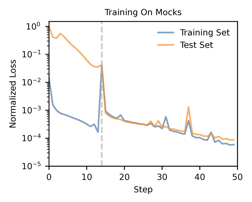
Figure 1: The learning curve (blue) for training the neural network along with the validiation loss (orange) on the test set at 49 steps. Each step corresponds to 100 epochs of training. The transition between the two training stages occurs at step 15, indicated by a vertical dashed line. The loss saturates by the end of the training.

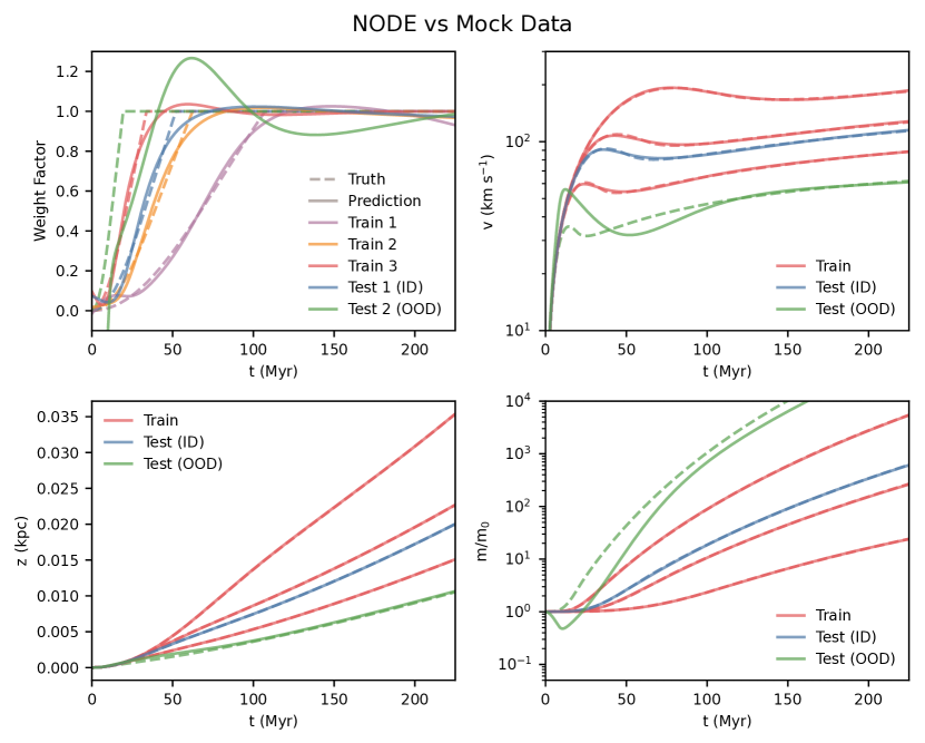
Figure 2: Comparison of neural ODE predictions against mock data. The four panels show (clockwise from top left): (a) Weight factor evolution, (b) Velocity evolution, (c) mass evolution, and (d) Distance fallen. Dashed lines represent the ground truth, while solid lines represent the neural ODE predictions. Each panel compares the two over a range of cloud sizes from within the training data and for test cloud sizes both in-distribution (ID) and outside-of-distribution (OOD) of the training data.

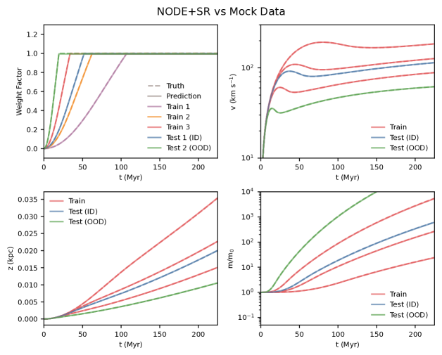
Figure 3: Same as Figure 2, but after applying Symbolic Regression to the neural ODE model. The SR model improves the predictive power of the neural ODE model, especially for out-of-distribution (OOD) test data. In this case SR recovers the ground truth equation used to generate the mock data.

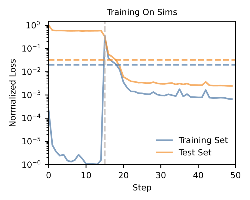
Figure 4: As in Figure 1, but for training the neural ODE model on actual simulation data. Horizontal dashed lines show the evaluation of the loss function between the simulation data and the model used in Tan et al. (2023) (Equation (4)).

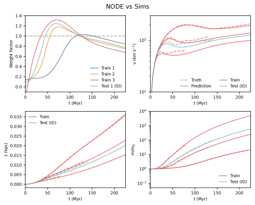
Figure 5: Comparison of neural ODE predictions against simulation data. Note there is no ‘ground truth’ for the weight factor in the simulations. Dashed lines show the more limited data from the simulations versus the mocks. The neural ODE model is able to capture the evolution of the weight factor well, but less so for the velocity. This is like due to model not accounting for drag well, in particular for the smaller clouds, which only affects the velocity directly.

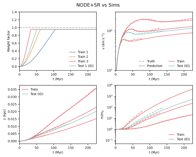
Figure 6: Same as Figure 5, but again after applying Symbolic Regression to the neural ODE model. Surprisingly, we recover a very similar equation to Equation (4), indicating that the original guess was a good one.

We first train on the mock data we generate to evaluate the performance of the neural ODE on a known hidden function. In Figure 1, we show the learning curve (in blue) for the training of the neural network, along with the validation loss (orange) on the test set at 49 steps. Each step corresponds to 100 epochs of training. The transition between the two training stages is indicated by a vertical dashed line. The initial loss of the training set is small since we only train on 20% of the full time series. The loss with respect to the training and test set are similar once we reach the second stage. The loss on the test set eventually saturates by the end of the training process, while the loss on the training set continues to decrease as the neural network begins to overfit to the training data.

In Figure 2, we show the comparison of the trained neural ODE predictions against the mock data. The four panels show the evolution of (clockwise from top left): the weight factor, the velocity, the cloud mass, and the total distance fallen. Dashed lines represent the ground truth generated by the assumed model, while solid lines represent the neural ODE predictions. Each panel compares the two over a range of cloud sizes from within the training data (red lines) and for test cloud sizes both in-distribution (ID, teal line) and outside-of-distribution (OOD, green line) of the training data. The neural ODE is able to reproduce the velocity, mass, and distance evolution of the training data well, and similarly so for test clouds with sizes that fall within the range of sizes spanned by the training data. We can see that this is directly reflected in the ability of the neural network to predict the weight factor. However, the neural ODE does a poorer job at predicting the weight factor and hence the mass, velocity and distance evolution for test clouds with sizes that are outside the range of the training data. This is not surprising — generalizing beyond the parameter space of the training data is a well-known challenge in scientific machine learning.

Understanding the physics of the system is also an important goal. To this end, we explore the application of Symbolic Regression to the neural ODE model. Since we are using a neural network in our ODE to model the influence of a specific process (in this context the development of turbulence in the mixing layers), we have defined the scope of the physical process the neural network is capturing. By doing this, it should be possible to use Symbolic Regression to discover the equation governing this process since we do not expect the underlying equation to be extremely complex. Of course, there is an implicit assumption here that the rest of the ODE is a good reflection of the physics of the rest of the system. If this is not the case, then the neural network might ‘learn’ things related to other parts of the system, which would muddy the interpretation.

In Figure 3, we show the results of applying Symbolic Regression to the neural ODE model. In this case, SR ‘discovers’ the ground truth equation used to generate the mock data (Equation (4)). Table 1 shows a comparison between the two equations, which are almost identical. The SR model hence improves the generalization of the neural ODE. It also makes the results interpretable — we are able to interpret the discovered equation as with any other physical equation we might have derived using traditional methods.

3.2 Training a Second Neural Network

We now train the neural ODE model on actual simulation data. In Figure 4, we show the learning curve for the training of the neural network on the simulation data. The training is less smooth compared to with the mock data. The loss is higher in the test set than the training set. This indicates there is more overfitting to the training data. The improvement in the loss also starts to saturate at a much earlier time. The horizontal dashed lines show the evaluation of the loss function between the simulation data and the model used in Tan et al. (2023) (Equation (4)). This shows that the neural ODE model is better able to capture the evolution of the weight factor or equivalently the mass growth rate in the simulations.

In Figure 5, we show the comparison of the trained neural ODE predictions against the simulation data. Simulation data is represented by the dashed lines. It can be seen that the data from the simulation is more limited for smaller clouds due to box sizes in the simulation. Since our loss function is based on the mass, the neural ODE model is able to capture the evolution of the mass well, but less so for the velocity. This is likely due to the model not accounting for drag well, which only affects the velocity directly, in particular for the smaller clouds,. Again, we are able to draw such conclusions due to the constrained scope of the neural network in our ODE. So although the predicted mass matches the simulation data well, the velocity profiles shows more deviation. This itself is useful information, as it indicates that we need to better model the drag in order to increase the fidelity of the model (whether analytically or with a neural network).

Dataset	True Equation	Learned Equation (SR)
Model	$\min\left(1,0.02\frac{z}{r}\right)$	$\min\left(0.9948299,0.01994161\frac{z}{r}\right)$
Simulation	-	$\min\left(0.95419395,0.01955151\frac{z}{r}\right)$

Table 1: Symbolic regression learned equations selected by best score.

In Figure 6, we show the results of again applying Symbolic Regression to the neural ODE model. In this case, SR still recovers a very similar equation to Equation (4), only with slightly different coefficients. The learned equation is shown in Table 1. While slightly surprising, this suggests that this was a good choice in the original work despite its simplicity. However, the predicted mass evolution is less accurate. In evaluating equations during Symbolic Regression, complexity is penalized. It is likely that this equation captures the essence of the physics of the system, but perhaps not higher order effects. This complexity penalty can be adjust to further explore equations which fit the data better but are more complex. These equations can then be analyzed for their physical relevance.

3.3 Performance on Simulation Data

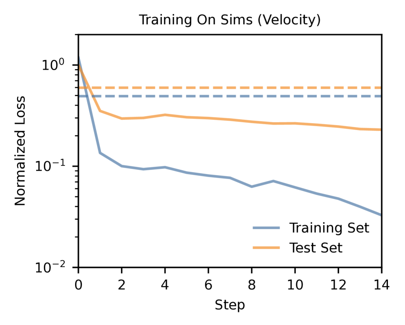
Figure 7: The loss curves during training of the second neural network to learn the drag coefficient. As in Figure 2, horizontal dashed lines show the evaluation of the loss function between the simulation data and the model used in Tan et al. (2023) (Equation (4)).

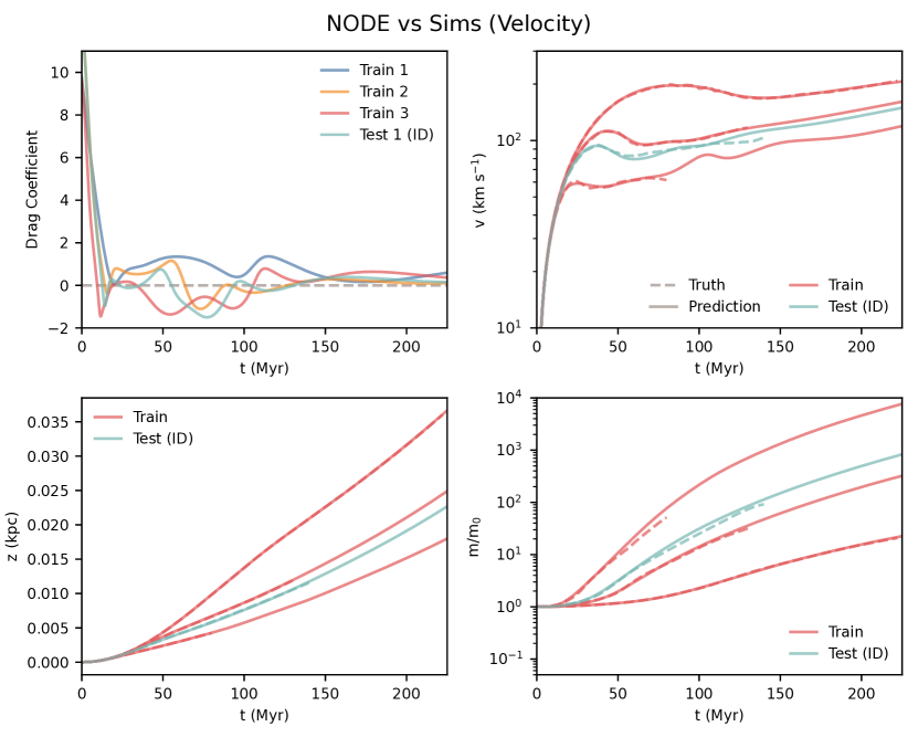
Figure 8: Results after training a second neural network to learn the drag coefficient over time, which is plotted in the top left panel. This quantity starts high and rapidly decreases to a small number. The total model now predicts the velocity evolution well. The mass predictions are only slightly less accurate.

Up to this point, we have trained a single neural network to learn the evolution of the weight factor describing the onset of turbulent mixing. However, as we noted above, our learned neural ODE does a good job in matching the mass evolution but differs from the data in its prediction for the velocity evolution (see Figure 5). We attributed this to firstly, designing a loss function that only takes into consideration the mass evolution (physically motivated by the fact that turbulent mixing only directly affects mass growth), and secondly, the simplification of the representation of conventional drag in our equations. This is the rightmost term in Equation (2), where we assume that the drag coefficient $C_{0}$ is a constant equal to unity. In reality, the drag coefficient is affected by a range of factors that can influence the amount of drag, and can vary with parameters such as velocity and geometry. Due to the complexity involved, the drag coefficient is usually measured experimentally in wind tunnel experiments. While this term is generally much smaller than accretion drag for growing clouds (Tan et al., 2023), we can further improve our subgrid model by repeating the process and replace $C_{0}$ with a second neural network.

We begin with the trained model from the previous section with the learned weight factor and freeze the parameters of that neural network. We then replace $C_{0}$, which was simply a constant of unity, with a second neural network. There are several changes we make in the training process for this network. Since the baseline model from the previous section already works well, we train on the full time evolutions from the start. We employ early stopping to avoid overfitting, and end the training when the loss on the test set stops improving. We thus train over 14 steps (1400 epochs). Figure 7 shows the training and validation loss over the training process. We adopt a similar loss function as before, but compute the loss with respect to the velocity instead of the mass, since $C_{0}$ only directly affects the clouds velocity. The results can be seen in Figure 8, which shows that the model does a better job at matching the velocity evolution (compared to Figure 5). The predictions for mass evolution have shifted a little bit since the equations are coupled, but not by much since the velocity changes are small. We could continue to iterate the training of the neural networks to further reduce the errors, but the improvements are likely to be incremental. Note that training separately makes training more efficient since we were able to use two separate loss functions, with the first neural network capturing the more important physical uncertainty in the system.

Once again, we run symbolic regression on the neural network to recover a physical expression for the drag coefficient. This gave the expression

$$C_{0}=\min(0.92/v,8.6).$$ (5)

We can see in the top left panel of Figure 8 the predicted time evolution of the drag coefficient for various clouds. They can be characterized by a initial rapid decline before saturating close to zero. The minimum in the learned function is due to the function $1/v$ diverging at $t=0$ when the cloud is at rest. This inverse scaling is consistent with a range of empirical data for spheres which find that the drag coefficient scales inversely with the Reynolds number, which itself scales linearly with velocity (Goossens, 2019). Furthermore, while the cloud begins as spherical object, it develops a long tail and becomes more streamlined as it falls and grows. We would hence expect the drag coefficient to approach some small value $<1$, which is consistent with the predictions of the neural network.

4 Discussion and Conclusion

For systems where the full range of scales cannot be resolved, as is common in astronomy, we rely on subgrid models to capture important unresolved processes. Using theory to derive differential equation models and testing them against simulations is the traditional method of constructing these models. We have shown that (at least in the context of galactic cloud-environment interactions) neural ODEs together with Symbolic Regression can be used to improve the predictive power of such models and better capture the complex physics involved. For our system, the trained neural ODE model can accurately capture the evolution of the weight factor, velocity, mass, and distance fallen for both mock data and simulation data. The is in spite of the small size of the training data. By leveraging modern software libraries, constructing and training of the neural ODE model is seamless and rapid. On the simulation data, the deviation of the model from observed velocities also indicates that there is room for improvement in modelling drag forces on the cloud, enabling us to identify deficiencies in other parts of the model. By embedding the neural network in the ODEs, we are able to constrain its scope of impact on the system. This makes the neural ODE model both interpretable and physically motivated, while still being flexible and predictive. It also allows us to effectively employ symbolic regression for scientific equation discovery. The model performs well on test data within the range of the training data but struggles with out-of-distribution test data. In this case, Symbolic Regression can be used to improve the generalization of the neural ODE model. For the mock data, SR recovers the ground truth equation used to generate the data. In the case of the simulation data, SR recovers a very similar equation to the one used in the original work. We also demonstrate that we can train multiple neural terms in the ode, each with physically tailored loss functions, and in order of physical importance. This not only further improves the predictive power of the model, but also increases the effectiveness of using symbolic regression to make physical insights.

It is important to highlight that the simulations we have run in this work are extremely idealized. In a more realistic setting with less idealized initial conditions, this time-dependent weight factor might be complicated, for example depending on turbulence inherent in the background seeded by other physical mechanisms such as extrinsic turbulence or cooling induced pulsations in the cloud (Gronke & Oh, 2020, 2022). A natural follow up would be to apply the methodologies explored in this work to these more realistic setups.

Nonetheless, we have shown how neural ODEs in tandem with Symbolic Regression are natural extensions of traditional methods of formulating subgrid or semi-analytic models and would be valuable parts of the modelling toolkit, both to develop more accurate subgrid models of complex systems and to enhance the scientific discovery process.

Data Availability

We make our code and all data used in this work public in a GitHub repository (github.com/zunyibrt/Neural-Infalling-Cloud-Equations).

References

- Begelman & Fabian (1990) Begelman M. C., Fabian A. C., 1990, MNRAS, 244, 26P
- Bradbury et al. (2018) Bradbury J., et al., 2018, JAX: composable transformations of Python+NumPy programs, http://github.com/google/jax
- Brunton et al. (2020) Brunton S. L., Noack B. R., Koumoutsakos P., 2020, Annual review of fluid mechanics, 52, 477
- Chen et al. (2018) Chen R. T. Q., Rubanova Y., Bettencourt J., Duvenaud D., 2018, arXiv e-prints, p. arXiv:1806.07366
- Chomiuk & Povich (2011) Chomiuk L., Povich M. S., 2011, AJ, 142, 197
- Cranmer (2023) Cranmer M., 2023, Interpretable Machine Learning for Science with PySR and SymbolicRegression.jl, doi:10.48550/arXiv.2305.01582, http://arxiv.org/abs/2305.01582
- Cranmer et al. (2020) Cranmer M., Sanchez-Gonzalez A., Battaglia P., Xu R., Cranmer K., Spergel D., Ho S., 2020, NeurIPS 2020
- Erb (2008) Erb D. K., 2008, ApJ, 674, 151
- Fielding & Bryan (2022) Fielding D. B., Bryan G. L., 2022, ApJ, 924, 82
- Fielding et al. (2020) Fielding D. B., Ostriker E. C., Bryan G. L., Jermyn A. S., 2020, ApJ, 894, L24
- Fraternali & Binney (2008) Fraternali F., Binney J. J., 2008, MNRAS, 386, 935
- Goossens (2019) Goossens W. R., 2019, Powder Technology, 352, 350
- Gronke & Oh (2018) Gronke M., Oh S. P., 2018, MNRAS, 480, L111
- Gronke & Oh (2020) Gronke M., Oh S. P., 2020, MNRAS, 494, L27
- Gronke & Oh (2022) Gronke M., Oh S. P., 2022, arXiv e-prints, p. arXiv:2209.00732
- Heckman & Thompson (2017) Heckman T. M., Thompson T. A., 2017, arXiv e-prints, p. arXiv:1701.09062
- Hopkins et al. (2008) Hopkins A. M., McClure-Griffiths N. M., Gaensler B. M., 2008, ApJ, 682, L13
- Hunter (2007) Hunter J. D., 2007, Computing in Science & Engineering, 9, 90
- Hwang et al. (2021) Hwang J., Choi J., Choi H., Lee K., Lee D., Park N., 2021, arXiv e-prints, p. arXiv:2111.06011
- Kidger (2022) Kidger P., 2022, arXiv e-prints, p. arXiv:2202.02435
- Kidger & Garcia (2021) Kidger P., Garcia C., 2021, Differentiable Programming workshop at Neural Information Processing Systems 2021
- Kim et al. (2021) Kim T. D., Luo T. Z., Pillow J. W., Brody C. D., 2021, in Meila M., Zhang T., eds, Proceedings of Machine Learning Research Vol. 139, Proceedings of the 38th International Conference on Machine Learning. PMLR, pp 5551–5561, https://proceedings.mlr.press/v139/kim21h.html
- Klein et al. (1994) Klein R. I., McKee C. F., Colella P., 1994, ApJ, 420, 213
- Kuwahara & Bauch (2023) Kuwahara B., Bauch C. T., 2023, medRxiv
- LeCun et al. (2015) LeCun Y., Bengio Y., Hinton G., 2015, Nature, 521, 436
- Nguyen (2023) Nguyen D. D., 2023, arXiv e-prints, p. arXiv:2306.11666
- Nguyen et al. (2023) Nguyen D. D., Ting Y.-S., Thompson T. A., Lopez S., Lopez L. A., 2023, arXiv e-prints, p. arXiv:2311.02057
- Putman et al. (2009) Putman M. E., et al., 2009, ApJ, 703, 1486
- Putman et al. (2012) Putman M. E., Peek J. E. G., Joung M. R., 2012, ARA&A, 50, 491
- Rackauckas et al. (2020) Rackauckas C., et al., 2020, arXiv e-prints, p. arXiv:2001.04385
- Rubin et al. (2014) Rubin K. H. R., Prochaska J. X., Koo D. C., Phillips A. C., Martin C. L., Winstrom L. O., 2014, ApJ, 794, 156
- Shapiro & Field (1976) Shapiro P. R., Field G. B., 1976, ApJ, 205, 762
- Smith et al. (2024) Smith M. C., et al., 2024, MNRAS, 527, 1216
- Söderlind (2003) Söderlind G., 2003, ACM Transactions on Mathematical Software, 20, 1
- Steidel et al. (2010) Steidel C. C., Erb D. K., Shapley A. E., Pettini M., Reddy N., Bogosavljević M., Rudie G. C., Rakic O., 2010, ApJ, 717, 289
- Stone et al. (2020) Stone J. M., Tomida K., White C. J., Felker K. G., 2020, ApJS, 249, 4
- Tan & Fielding (2024) Tan B., Fielding D. B., 2024, MNRAS, 527, 9683
- Tan et al. (2021) Tan B., Oh S. P., Gronke M., 2021, MNRAS, 502, 3179
- Tan et al. (2023) Tan B., Oh S. P., Gronke M., 2023, MNRAS, 520, 2571
- Tsitouras (2011) Tsitouras C., 2011, Computers & Mathematics with Applications, 62, 770
- Van Der Walt et al. (2011) Van Der Walt S., Colbert S. C., Varoquaux G., 2011, Computing in Science & Engineering, 13, 22
- Veilleux et al. (2005) Veilleux S., Cecil G., Bland-Hawthorn J., 2005, ARA&A, 43, 769