Empirical risk minimization for risk-neutral composite optimal control with applications to bang-bang control111Funding: This material is based upon work supported by the National Science Foundation under Grant No. DMS-2410944.
Abstract
Nonsmooth composite optimization problems under uncertainty are prevalent in various scientific and engineering applications. We consider risk-neutral composite optimal control problems, where the objective function is the sum of a potentially nonconvex expectation function and a nonsmooth convex function. To approximate the risk-neutral optimization problems, we use a Monte Carlo sample-based approach, study its asymptotic consistency, and derive nonasymptotic sample size estimates. Our analyses leverage problem structure commonly encountered in PDE-constrained optimization problems, including compact embeddings and growth conditions. We apply our findings to bang-bang-type optimal control problems and propose the use of a conditional gradient method to solve them effectively. We present numerical illustrations.
Key words. bilinear control,
sample average approximation,
empirical risk minimization,
PDE-constrained optimization,
stochastic optimization,
bang-bang control
AMS subject classifications. 90C15, 90C59, 90C06, 35Q93, 49M41, 90C60
1 Introduction
In this paper, we consider composite risk-neutral optimization problems of the form
| () |
is a compact linear operator between the Hilbert space and the Banach space , is a smooth integrand, and is a proper, closed, and convex but potentially nonsmooth. Moreover, denotes a random element, which maps to a complete, separable metric space . While () covers a variety of challenging settings, the focus of the present work lies on risk-neutral PDE-constrained optimal control problems
| (1.1) |
where is a tracking-type functional, and the choice of the deterministic control influences the behavior of the solution to a PDE with random inputs .
Nonconvex optimization problems governed by differential equations arise in a multitude of application areas, such as sensor placement [2], resource assessment of renewable tidal energy [8], and design of groundwater remediation systems [9]. It is well known that the proper choice of the penalty function in Problem 1.1 promotes certain structural features in its minimizers . For example, setting
denotes its indicator function, and , tends to provide solutions satisfying a bang-bang-off principle, that is, for a.e. . As a consequence, composite optimal control problems also arise from relaxations of mixed-integer optimal control problems [8].
In order to handle the expected value in () numerically, we approximate it using the sample average approximation (SAA) approach [12]. More specifically, given a sequence defined on a complete probability space of independent -valued random elements such that each has the same distribution as , we consider the SAA problem
| () |
For brevity, we often omit the second argument of .
A central topic arising in this context is the question whether this type of approximation is asymptotically consistent and if the proximity of its solutions and critical points towards their counterpart in () can be quantified in terms of the sample size . Although this already represents a formidable problem for smooth objective functions, the potential lack of strong convexity of aggravates the problem further, adding additional challenges to the theoretical analysis of the problem and its efficient solution.
1.1 Contributions
In the present paper, we investigate the SAA approach for nonsmooth, potentially nonconvex risk-neutral minimization problems of the form () from a qualitative and a quantitative perspective. Since Problem () is potentially nonconvex, our analysis addresses the behaviour its solutions and its critical points. In the context of the present manuscript, the latter refers to points satisfying the first-order necessary subdifferential inclusion
or, equivalently, zeros of the gap functional
| (1.2) |
Critical points as well as the associated gap function for Problem () are defined analogously. More specifically, the contributions of the paper are as follows:
- (a)
-
(b)
We establish nonasymptotic expectation bounds for the gap functional value of arbitrary sequences of random vectors. More precisely, we demonstrate that, for every there holds
where , , denotes the -covering number of the compact set and explicitly depends on the radius of the domain of as well as the smoothness of the integrand .
-
(c)
While Problem () is typically not strongly convex, we provide nonaymptotic expectation bounds for the approximation of minimizers to () by random vectors realizing solutions of Problem () if the integrand is convex for each , and a growth-type condition on the partial linearization of at a minimizer holds true. Specifically, if
(1.3) for some and a Banach space with , then
where depends on the smoothness of the integrand, and . Hence, the SAA solutions converge in expectation at the usual Monte Carlo rate of while both the value of the gap functional and the suboptimality in exhibit superconvergence at a rate of . This convergence statement is valid for linear bounded operators without their compactness.
Our framework is applied to PDE-constrained optimization problems governed by affine-linear and bilinear elliptic equations, which allow for the use of bang-bang-off regularization terms. Reproducible numerical experiments empirically verify our theoretical results and further highlight the utility of the SAA approach for infinite-dimensional, nonsmooth problems.
1.2 Related work
Monte Carlo sample-based approximations are common discretization approaches for risk-neutral and risk-averse huge-scale optimization, particularly in PDE-constrained optimization [19], and stochastic optimization [34]. The theoretical analyses of this approximation approach may be categorized into asymptotic and nonasymptotic ones. In PDE-constrained optimization under uncertainty with strongly convex control regularizers, the papers [11, 18, 20, 31] provide nonasymptotic analyses, such as sample size estimates and central limit-type theorems. Moreover, [19, 24, 25] provide asymptotic consistency results for nonconvex infinite-dimensional stochastic optimization. The problem structure given by the compact linear operator in (4.1) is common among PDE-constrained optimization problems and has been used for different purposes in the literature. For example, the authors of [25] have employed it to demonstrate the consistency of empirical estimators for risk-averse stochastic optimization. Finally, [26] establishes nonasymptotic sample size estimates for risk-neutral semilinear PDE-constrained optimization. In the field of PDE-constrained optimization under uncertainty, current SAA analyzes require certain control regularizers, such as standard Tikhonov regularizers [11, 21], R-functions [25], and Kadec functions [24]. These requirements exclude the -norm as a control regularizer, for example. Using the problem structure given by the compact linear operator in (4.1), we are able to extend previous results to general convex control regularizers.
As mentioned in the previous section, our sample size estimates for convex problems do not depend on the compactness of the feasible set or of the operator . Sample size estimates for stochastic convex optimization without any compactness conditions are also established, for example, in [15, 21, 33].
1.3 Outline
Section 2 introduces notation and terminology. Section 3 introduces assumptions on the risk-neutral composite control problems, studies the existence of solutions, states gap functional-based optimality conditions, and establishes consistency of SAA optimal values, solutions and critical points. Section 3 also derives sample size estimates for nonconvex and convex problems. Our framework is applied to linear and bilinear PDE-constrained optimization in section 4. Section 5 presents numerical illustrations. The appendix derives uniform expectation bounds.
2 Notation and terminology
Throughout the text, normed vector spaces are defined over the reals. Metric spaces are equipped with their Borel sigma-field . Moreover, we identify the control space , a separable Hilbert space, with , and write . For a Banach space with norm , we denote by its topological dual space and by its duality pairing. If the norm is clear from the context, we write instead of . The inner product on a Hilbert space is denoted by . If and are Banach spaces with , and defined by is linear and bounded, then we say that is (continuously) embedded into . We abbreviate such embeddings by . A linear operator between two Banach spaces is called compact if its image of the domain space’s unit ball is precompact. For a linear bounded operator between Banach spaces, denotes its adjoint operator. For a measurable space and metric spaces and , is called Carathéodory mapping if is continuous for all and is - measurable for all . For a bounded domain , we denote by the standard Lebesgue spaces, and by and ( the standard Sobolev spaces. We set . For a nonempty, totally bounded metric space , the -covering number , , denotes the minimal number of points in a -net of .
3 Risk-neutral composite optimal control
We start by stating the main assumptions on Problem (). For this purpose, we abbreviate the domain of by
The following assumption imposes the properties of and the smoothness and integrability requirements on the integrand.
Assumption 1 (Integrand and feasible set).
-
(a)
The control space is a separable Hilbert space, and is a separable Banach space.
-
(b)
The operator is linear, and compact.
-
(c)
The function is proper, closed, convex, and is bounded.
-
(d)
The set is open, convex, and bounded with . Moreover, is continuous in its first argument on for each and measurable in its second argument on for each .
-
(e)
For an integrable random variable , it holds that
The following assumption formulates differentiablity and integrability statements of derivatives.
Assumption 2 (Integrand and its gradient).
-
(a)
For each , the mapping
is continuously differentiable.
-
(b)
There exists a Carathéodory function such that
-
(c)
There exists an integrable random variable such that
If is continuously differentiable on a -neighborhood of , the differentiability of and the representation of its gradient are implied by the chain rule. From this perspective, Assumption 2 will ensure that the gradients of and admit a composite structure even in the absence of the chain rule. While this might seem technical at first glance, it will allow us to fit challenging settings into the outlined abstract framework. For a particular example, we refer the reader to the bilinear PDE-constrained problem in section 4.2.
3.1 Existence of solutions and necessary optimality conditions
In this section, we show that both the risk-neutral problem () and the associated SAA problems () admit solutions. We also show the measurability of the SAA optimal value and the existence of measurable SAA solutions. Moreover, we introduce the particular form of first-order necessary optimality conditions used in the following sections.
Proposition 3.1.
Let Assumption 1 hold, and let . Then, (i) the risk-neutral problem () and for each , the SAA problem () admit solutions, (ii) the function is measurable, and (iii) there exists at least one measurable map such that for each , solves the SAA problem (). (iv) If, moreover, LABEL: and 2 holds, then the composite functions and are continuously differentiable on with gradients and , respectively.
Proof.
(i) Since is weakly compact, the proof follows by standard arguments as well as Fatou’s lemma.
(ii)–(iii) Since is Carathéodory on , measurability theorems on marginal maps and inverse images [4, Thms. 8.2.9 and 8.2.11] imply the assertions.
(iv) The assertions can be established using standard arguments. ∎
Propositions 3.1 and 2 motivate the definitions
as mappings on and , respectively. We note that these definitions are formal in the sense that while is well-defined, may not be continuously differentiable, see also the discussion following Assumption 2. As with , we often omit the second argument of .
Furthermore, we define the gap functionals and by
| (3.1) |
A point is referred to as critical point of () if . Similarly, a point is called a critical point of the SAA problem () if . Critical points of () are the zeros of the gap function as summarized in the following proposition.
Proposition 3.2.
If Assumptions 1 and 2 hold, then (i) an element is a critical point of () if and only if , (ii) a point is a critical point of () if and only if , and (iii) is weakly lower semicontinuous.
3.2 Consistency of SAA optimal values and solutions
We establish the asymptotic consistency of SAA optimal values and the weak consistency of SAA solutions. We denote by the optimal value of the true problem ().
Theorem 3.3.
If Assumption 1 holds, then (i) as w.p. , and (ii) for almost all , has at least one weak accumulation point in and every such point is a solution to ().
Proof.
Before we establish parts (i) and (ii), let us note that the uniform law of large numbers [14, Cor. 4:1] ensures the existence of a null set with such that for all , we have
| (3.2) |
Moreover, is continuous on owing to the dominated convergence theorem.
(ii) Fix . Since is bounded, it has a weak accumulation point. Let be a weak accumulation point of . By assumption, there exists a subsequence of such that as . Fix . We have
Using the convergence statement in (3.2), and as , we obtain and as . Combined with the fact that is weakly lower semicontinuous,
Since occurs w.p. , we obtain the assertion. ∎
3.3 Consistency of SAA critical points
We establish the asymptotic consistency of the SAA gap functional evaluated as approximate SAA critical points as well as that of SAA critical points.
Theorem 3.4.
Let Assumptions 1 and 2 hold, and let be a sequence with as . Let be a sequence of random vectors with w.p. . Then (i) as w.p. . (ii) For almost all , has at least one weak accumulation point in and every such point is a zero of .
Proof.
Before we establish parts (i) and (ii), let us note that for all ,
| (3.3) |
Hence, we have for all ,
| (3.4) |
Therefore, the uniform law of large numbers [14, Cor. 4:1] ensures the existence of a null set with such that for all , we have
(i) Using , the error bound (3.4), and the above convergence statement, we obtain as w.p. .
(ii) Fix such that as . Since is bounded, it has a weak accumulation point. If as , then the weak lower semicontinuity of established in Proposition 3.2) and as imply the assertion. ∎
3.4 Sample size estimates for SAA critical points
We establish expectation bounds and sample size estimates. Our analysis is inspired by that of [34].
For this purpose, we formulate a Lipschitz continuity assumption and a light-tailed condition on the integrand’s gradient, which are a typical assumptions in related contexts.
Assumption 3 (Lipschitz-type condition on integrand’s derivative, sub-Gaussian derivatives).
-
(a)
For an integrable random variable ,
-
(b)
For some constant ,
3 (b) is, for example, satisfied if there exists a constant such that for all . We denote by the diameter of .
Theorem 3.5.
Let Assumptions 1, 2 and 3 hold. For each , let be measurable. Then, for all and ,
| (3.5) |
Proof.
Using Theorem 3.5, we establish sample size estimates.
Corollary 3.6.
Proof.
The sample size estimates in Corollary 3.6 are based on the covering numbers of . A typical example in PDE-constrained optimization models as the adjoint operator of the embedding . Combining the covering numbers for Sobolev function classes in [6, Thm. 1.7] and duality of metric entropy [3, p. 1315], covering numbers of can be derived.
3.5 Expectation bounds for convex problems
For convex problems, we demonstrate nonasymptotic expectation bounds for the distance between SAA solutions and the true solution, the gap functional, and the optimality gap. These statements hold true without the compactness of the linear bounded operator . In the following, let be a solution to () and for each , let be a measurable solution to ().
Assumption 4 (Hölder-type inequality, gradient regularity, growth, and standard deviation).
-
(a)
The space is a Banach space with , is a separable Hilbert space with , and
-
(b)
For two constants and , it holds that
-
(c)
The mapping is integrable, and standard deviation-type constant
is finite.
4 (b) and its variants have been utilized, for example, in [13] and, in particular, ensures that is the unique solution to ().
We state the section’s main result. If 4 (a) holds true, let be the embedding constant of the embedding . If in Assumption 4, the following result ensures the typical Monte Carlo convergence rate, , for the expected error .
Theorem 3.7.
If Assumptions 1, 2 and 4 hold, and is convex for all , then for all ,
Proof.
The proof is inspired by those of Lemma 6 and Theorem 3 in [21]. Using and 4 (b), we obtain
Since is continuously differentiable on (see Proposition 3.1), and convex, we have
Adding both estimates ensures
Hence
Taking squares and using the continuity of the embedding , we obtain
Since (see Proposition 3.1), , are independent and identically distributed, and is a separable Hilbert space, we obtain
| (3.6) |
This implies the expectation bound. ∎
Using this result, we further deduce superconvergence properties of the objective function values and the gap functional evaluated at SAA solutions. We recall that denotes the objective function of ().
Corollary 3.8.
Let the hypotheses of Theorem 3.7 hold with , and assume that there exists such that
| (3.7) |
Then, for all , we have
Proof.
Since for all (see, for example, [13, Thm. 2.4]), it suffices to show the claimed estimate for the gap functional. For this purpose, note that there exists such that
where the first inequality follows from the optimality of . Using (3.7), we have
Following the proof of Lemma 4.8 in [13], we arrive at
where the final inequality is due to (3.7). Putting together the pieces, we have
Taking expectations, and using (3.6) and Theorem 3.7, we obtain the expectation bound. ∎
4 Application to bang-bang optimal control under uncertainty
In this section, we apply our results to risk-neutral, nonsmooth PDE-constrained minimization problems of the form
| (4.1) |
where , , is a bounded, polyhedral domain, , is a smooth fidelity term defined on and denotes the compact embedding. Moreover,
The deterministic control is coupled with the random state variable via a parametrized elliptic PDE
| (4.2) |
which the state satisfies for every . Throughout this section, we consider
In the following, we show that both linear, that is, , as well as bilinear, that is, , control problems fit into the theoretical framework () defining
as well as introducing the integrand
| (4.3) |
denotes a suitable parametrized control-to-state operator defined on the image of a -neighborhood of . For both problem classes, the following assumptions are made.
Assumption 5 (Fidelity term, PDE right-hand side, random diffusion coefficient).
-
(a)
The function is convex and continuously differentiable. Its gradient is Lipschitz continuous with Lipschitz constant . Moreover for all , where is a polynomial and nondecreasing.
-
(b)
The map is measurable and there exists such that for all .
-
(c)
The mapping is measurable and for all . Moreover, there exists such that for all and .
We point out that 5 (a) implies
| (4.4) |
Moreover, 1 (a), 1 (b) and 1 (c) are clearly satisfied. For abbreviation, let be the Friedrichs constant of the domain , which equals the operator norm of .
4.1 Risk-neutral affine-linear PDE-constrained optimization
We first consider (4.1) governed by a class of affine-linear, parameterized PDEs, that is, . For simplicity, set . We consider the operator
where
and the associated parametrized equation
| (4.5) |
The following lemma is a direct consequence of the Lax–Milgram lemma, the implicit function theorem as well as standard regularity results for elliptic PDEs. Its proof is omitted for the sake of brevity.
Lemma 4.1.
Let Assumption 5 hold with . For every , there exists a unique satisfying (4.5). The mapping is infinitely many times continuously differentiable, and we have
| (4.6) |
Moreover, if , then , and there exists a constant such that
| (4.7) |
Finally, the mapping
is continuous.
In the following, let be an arbitrary but fixed convex, bounded neighborhood of , and let be such that for all . Defining the parametrized control-to-state operator
we can verify the remaining assumptions in the linear case.
Lemma 4.2.
If Assumption 5 hold with , then in (4.3) is Carathéodory, and
Proof.
Next, we verify Assumptions 2 and 5 (a).
Lemma 4.3.
Let Assumption 5 hold with . We define
The mapping is Carathédoroy and, for every , the function
is continuously differentiable on with . Moreover, we have the estimates
Finally, we have
Proof.
The Carathéodory property of follows analogously to Lemma 4.2. Moreover, the differentiability of and the representation of its gradient are direct consequences of the chain rule as well as standard adjoint calculus, respectively. Using this representation and (4.6), we obtain
Furthermore, by applying (4.4), we have
| (4.8) |
where the last inequality follows again by using (4.6). Combining both inequalities yields the desired estimate. The Lipschitz estimate for follows analogously noting that
and thus
for all and . ∎
Next, we discuss sufficient conditions for Assumption 4 with the particular choice of and . In this case, 4 (a) is satisfied. In the following, we denote by a solution to (4.1). We recall the identity .
Proposition 4.4.
Let Assumption 5 hold with . Then, the mapping is measurable, and
If, moreover, there exist constants and such that
then there exists such that
Proof.
Finally, we comment on the uniform Lipschitz continuity assumed in Corollary 3.8.
Lemma 4.5.
Let Assumption 5 hold with . Assume that the mapping from 5 (c) satisfies all and some . Then, there holds
where is the constant from Lemma 4.1, and denotes the embedding constant of .
4.2 Risk-neutral bilinear PDE-constrained optimization
Next, we show that bilinear control problems, that is, , also fit our abstract setting. For this purpose, we assume for a.e. . Similar to the previous example, consider the operator
where
We readily verify that is infinitely many times continuously differentiable. Now, define the open set
where
Moreover, is the open -unit ball, and is the embedding constant of . We consider the equation
| (4.9) |
The following result is a consequence of the implicit function theorem. The constant in the following lemma is equal to that in Lemma 4.1.
Lemma 4.6.
Let Assumption 5 hold with for a.e. . For every , there exists a unique satisfying (4.9). The mapping is infinitely many times continuously differentiable, and we have
| (4.10) |
Moreover, if , then , we have
| (4.11) |
and the mapping
is continuous.
Proof.
Given , the existence of a unique solution to (4.9) and the a priori estimate in (4.10) follow from the Lax–Milgram lemma and the definitions of and , see also [24, sect. 7.1]. Similarly, the higher regularity and the estimate in (4.11) follow by a standard bootstrapping argument. It remains to discuss the regularity of the solution mapping. Starting with the -result, note that there holds
Together with (4.10), this implies that is a Banach space isomorphism. Hence, the smoothness of with respect to its inputs follows from the implicit function theorem. In order to verify the -continuity, let
denote two admissible triples and let be the associate solutions of (4.9). The difference is the unique solution of
where we identify
Invoking (4.11), we thus get
and together with
for some , the claimed continuity result follows. ∎
From this point on, we would like to argue as in the previous section by introducing an appropriate control-to-state operator in order to define the integrand . In the bilinear setting, however, this requires additional care, as the equation in (4.9) might not be well-posed for controls in a -neighborhood of . Taking this into account, we set and consider the mapping
Here, is the restriction of the compact operator , and denotes is noncontinuous inverse. Using the following lemma, we deduce the Lipschitz continuity of with respect to the control.
Lemma 4.7.
If is a bounded domain, then there exists a constant such that for all and , we have and
Proof.
This is a consequence of Theorem 7.4 in [5], the -trace operator’s continuity, and Friedrichs’ inequality. ∎
Lemma 4.8.
Let Assumption 5 hold with for a.e. . If and , then
| (4.12) |
Proof.
The following lemma verifies Assumption 1 for the integrand in (4.3).
Lemma 4.9.
Let Assumption 5 hold with for a.e. . Then
Moreover, is continuous in its first argument on for each and measurable in its second argument on for each .
Proof.
Next, we verify Assumptions 2 and 3 (a). We define
Lemma 4.10.
Let Assumption 5 hold with for a.e. . For each , consider the mapping
The function is continuous differentiable on , and there holds
Moreover, for every , we have , the mapping
is Carathéodory, and we have the a priori estimates
as well as for all ,
Moreover, there exists an integrable random variable such that
Proof.
The statement on the differentiability of is a direct consequence of the chain rule and adjoint calculus. If , then Lemma 4.6 implies and thus, see Lemma 4.7, . The Carathéodory property of follows again from the continuity of and . Invoking the stability estimates of Lemma 4.6, we further obtain
for all , and
| (4.13) |
As a consequence, we obtain
for all . Moreover, if , then
In particular, owing to Assumption 5, (4.11) and (4.13), there exists a square integrable random variable such that
as well as
In order to establish the claimed Lipschitz continuity, fix and , and split
For estimating the norm of the first difference, we note that
using Lemma 4.8. Similarly, arguing along the lines of proof in Lemma 4.8, we get
As a consequence, we have
Finally, we decompose and estimate
for some . By Friedrichs’ inequality, the claimed Lipschitz statement follows. ∎
Lemma 4.10 verifies Assumptions 2 and 3 (a). Moreover, as in the linear setting, 3 (b) is satisfied since is uniformly bounded on .
5 Numerical illustrations
We present numerical illustrations for two instances of the risk-neutral problems analyzed in section 4. The section’s main objective is to illustrate the theoretical results established in sections 3.4 and 3.5. Before presenting numerical results, we discuss problem data, discretization aspects, implementation details, and the computation of reference solutions and gap functions.
Problem data
We chose , the deterministic in (4.2), and in (4.1) with . For the random diffusion coefficient , we used a truncated Karhunen–Loève expansion with the eigenpairs described in Example 7.56 of [17]. Our truncated expansion includes addends, uses correlation length of , and independent truncated normal random variables each without shift, a standard deviation , and a truncation interval of . The remaining problem data are problem-dependent and introduced in sections 5.1 and 5.2.
Reference solutions and gap functions
As the risk-neutral problems considered in section 4.1 may lack closed-form solutions, we compute reference solutions. We constructed samples using a fixed realization of a scrambled Sobol’ sequence, generated using scipy’s quasi-Monte Carlo engine [32]. These samples are transformed via the inverse transformation method and their subsequent values referred to reference samples. We used these samples to define a reference problem. This reference problem is an SAA problem defined by the reference samples with . We refer to its solutions/critical points as reference SAA solutions/critical points. Moreover, we approximate the gap functional in (3.1) using the gap functional corresponding to the reference SAA problem. Similarly, we approximate the objective function via .
Discretization and implementation details
To obtain finite-dimensional optimization problems suitable for numerical solution, we discretized the state space using piecewise linear continuous finite element functions and using piecewise constant functions. These functions are defined on a regular triangulation of with being the number of cells in each direction. We refer to
as the nominal problem to (). We solved the discretized problems using a conditional gradient method [13]. Our implementation is archived at [22]. The method stops when the gap functional falls below or after 100 iterations, whichever comes first. Our simulation environment is built on dolfin-adjoint [7, 27], FEniCS [1, 16], and Moola [28]. The numerical simulations, except those for the nominal problems, were performed on the PACE Phoenix cluster [29]. The code and simulation output are archived at [23].
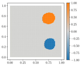
5.1 Affine-linear problem
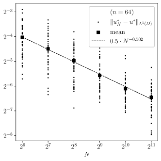
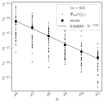
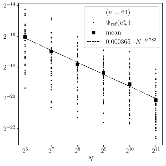
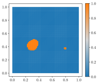
We chose , , and . Figure 1 depicts nominal solution and a reference SAA solution. Figure 2 depicts convergence rates for empirical estimates of the optimality gap and over the sample size . We used realizations to estimate these means, and computed convergence rates using least squares. Figure 3 depicts convergence rates of the SAA gap function’s empirical means. The empirical convergence rates closely match the theoretical ones.
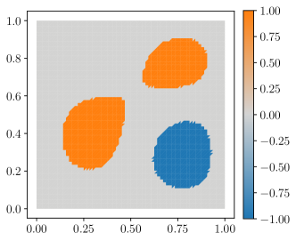
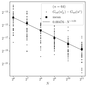
5.2 Bilinear problem
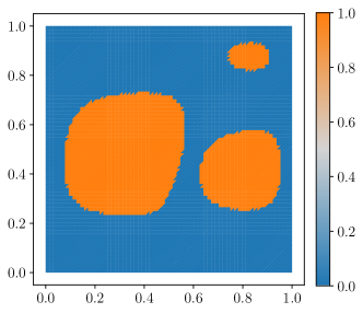
We chose the constant control bounds and , and . Figure 4 depicts nominal critical points and a reference SAA critical point. Figure 3 depicts convergence rates of the SAA gap function’s empirical means. These rates are faster than predicted by the theory, see Corollary 3.6. We think that this can be attributed to the fact that the covering number ansatz does not exploit higher-order regularity of the integrand and, in particular, potential local curvature around isolated minimizers. While a closer inspection of this improved convergence behavior is certainly of interest, it goes beyond the scope of the current work and is left for future research.
6 Discussion
In this paper, we have analyzed the SAA approach for risk-neutral optimization problems that incorporate a nonsmooth but convex regularization term. Our main results address the asymptotic consistency of this scheme, and the derivation of nonasymptotic sample size estimates for various optimality measures. The latter, as well as the employed techniques, come in two different flavours: for the general nonconvex case, we provide estimates on the expected value of the gap functional by applying the covering number approach. For convex objectives, and by relying on common growth conditions, we prove stronger results including convergence rates for the expected distance between minimizers, improved estimates for the gap functional, and the suboptimality in the objective function value. The presented abstract framework is applied to both linear and bilinear PDE-constrained problems under uncertainty. We also use these applications to empirically verify the sharpness of our convergence guarantees.
Our investigation also raises new questions about the SAA approach for nonsmooth minimization problems. These include, for example, the extension of the results in section 3.5 to nonconvex problems assuming suitable second-order optimality conditions and taking into account the potential existence of multiple global and/or local minimizers. Moreover, an extension of the current results to risk-averse stochastic optimization and variational inequalities may be of interest.
Reproducibility of computational results
Computer code that allows the reader to reproduce the computational results in this manuscript is available at https://doi.org/10.5281/zenodo.13336970.
Appendix A Uniform expectation bounds for expectation mappings
We establish essentially known uniform expectation bounds for integrands defined on potentially infinite-dimensional spaces. While the techniques used in this section are standard in the literature on stochastic programming, the bounds are instrumental for establishing one of our main result in section 3.4.
Let be a complete probability space, and let be a random element with image space . Moreover, let be sequence of independent -valued random elements defined on a complete probability space, each having the same distribution as .
Assumption 6 (sub-Gaussian Carathéodory function, compact linear operator).
-
(a)
The set is a nonempty, closed, bounded, convex subset of a reflexive Banach space , is a Banach space, and is linear and compact.
-
(b)
The space is a separable Hilbert space, and is a Carathéodory function.
-
(c)
For an integrable random variable , is Lipschitz continuous with Lipschitz constant for each .
-
(d)
There exists such that for all , we have .
We define , , and .
Proposition A.1.
If Assumption 6 holds, then for each and ,
Proof.
The proof is inspired by those of Theorems 9.84 and 9.86 in [34]. We have and for all , where . We define . Since is compact, is finite and there exist such that for each , we have , where . For all ,
Hence
Using Theorem 3 in [30] and Lemma 1 in [21], we have
Now, Lemma B.5 in [26] ensures . Combined with , we obtain the expectation bound. ∎
References
- [1] M. S. Alnæs, J. Blechta, J. Hake, A. Johansson, B. Kehlet, A. Logg, C. Richardson, J. Ring, M. E. Rognes, and G. N. Wells. The FEniCS Project Version 1.5. Arch. Numer. Software, 3(100):9–23, 2015. doi:10.11588/ans.2015.100.20553.
- [2] H. An, B. D. Youn, and H. S. Kim. Optimal sensor placement considering both sensor faults under uncertainty and sensor clustering for vibration-based damage detection. Struct. Multidiscip. Optim., 65(3):Paper No. 102, 32, 2022. doi:10.1007/s00158-021-03159-9.
- [3] S. Artstein, V. Milman, and S. J. Szarek. Duality of metric entropy. Ann. of Math. (2), 159(3):1313–1328, 2004. doi:10.4007/annals.2004.159.1313.
- [4] J.-P. Aubin and H. Frankowska. Set-Valued Analysis. Springer, Boston, 2009. doi:10.1007/978-0-8176-4848-0.
- [5] A. Behzadan and M. Holst. Multiplication in Sobolev spaces, revisited. Ark. Mat., 59(2):275–306, 2021. doi:10.4310/arkiv.2021.v59.n2.a2.
- [6] M. Š. Birman and M. Z. Solomjak. Quantitative Analysis in Sobolev Imbedding Theorems and Applications to Spectral Theory. AMS, Providence, RI, 1980. doi:10.1090/trans2/114.
- [7] S. W. Funke and P. E. Farrell. A framework for automated PDE-constrained optimisation. preprint, https://arxiv.org/abs/1302.3894, 2013.
- [8] S. W. Funke, S. C. Kramer, and M. D. Piggott. Design optimisation and resource assessment for tidal-stream renewable energy farms using a new continuous turbine approach. Renew. Energ., 99:1046–1061, 2016. doi:10.1016/j.renene.2016.07.039.
- [9] J. Guan and M. Aral. Optimal remediation with well locations and pumping rates selected as continuous decision variables. Journal of Hydrology, 221(1):20–42, 1999. doi:10.1016/S0022-1694(99)00079-7.
- [10] R. Herzog and F. Schmidt. Weak lower semi-continuity of the optimal value function and applications to worst-case robust optimal control problems. Optimization, 61(6):685–697, 2012. doi:10.1080/02331934.2011.603322.
- [11] M. Hoffhues, W. Römisch, and T. M. Surowiec. On quantitative stability in infinite-dimensional optimization under uncertainty. Optim. Lett., 15(8):2733–2756, 2021. doi:10.1007/s11590-021-01707-2.
- [12] A. J. Kleywegt, A. Shapiro, and T. Homem-de Mello. The sample average approximation method for stochastic discrete optimization. SIAM J. Optim., 12(2):479–502, 2002. doi:10.1137/S1052623499363220.
- [13] K. Kunisch and D. Walter. On fast convergence rates for generalized conditional gradient methods with backtracking stepsize. Numer. Algebra Control Optim., 14(1):108–136, 2024. doi:10.3934/naco.2022026.
- [14] L. M. Le Cam. On some asymptotic properties of maximum likelihood estimates and related Bayes’ estimates. Univ. California Publ. Stat. 1, pages 277–329, 1953. URL: https://hdl.handle.net/2027/wu.89045844305.
- [15] H. Liu and J. Tong. New sample complexity bounds for sample average approximation in heavy-tailed stochastic programming. In Forty-first International Conference on Machine Learning, 2024.
- [16] A. Logg, K.-A. Mardal, and G. N. Wells, editors. Automated Solution of Differential Equations by the Finite Element Method: The FEniCS Book. Springer, Berlin, 2012. doi:10.1007/978-3-642-23099-8.
- [17] G. J. Lord, C. E. Powell, and T. Shardlow. An Introduction to Computational Stochastic PDEs. Cambridge University Press, Cambridge, 2014. doi:10.1017/CBO9781139017329.
- [18] M. Martin, S. Krumscheid, and F. Nobile. Complexity analysis of stochastic gradient methods for PDE-constrained optimal control problems with uncertain parameters. ESAIM Math. Model. Numer. Anal., 55(4):1599–1633, 2021. doi:10.1051/m2an/2021025.
- [19] J. Milz. Consistency of Monte Carlo estimators for risk-neutral PDE-constrained optimization. Appl. Math. Optim., 87(57), 2023. doi:10.1007/s00245-023-09967-3.
- [20] J. Milz. Reliable Error Estimates for Optimal Control of Linear Elliptic PDEs with Random Inputs. SIAM/ASA J. Uncertain. Quantif., 11(4):1139–1163, 2023. doi:10.1137/22M1503889.
- [21] J. Milz. Sample average approximations of strongly convex stochastic programs in Hilbert spaces. Optim. Lett., 17:471–492, 2023. doi:10.1007/s11590-022-01888-4.
- [22] J. Milz. milzj/fw4pde: v1.0.2, February 2024. doi:10.5281/zenodo.10644778.
- [23] J. Milz. Supplementary code for the manuscript: Empirical risk minimization for risk-neutral composite optimal control with applications to bang-bang control, August 2024. doi:10.5281/zenodo.13336970.
- [24] J. Milz. Consistency of sample-based stationary points for infinite-dimensional stochastic optimization. preprint, https://arxiv.org/abs/2306.17032, June 2023.
- [25] J. Milz and T. M. Surowiec. Asymptotic consistency for nonconvex risk-averse stochastic optimization with infinite dimensional decision spaces. Math. Oper. Res., 2023. doi:10.1287/moor.2022.0200.
- [26] J. Milz and M. Ulbrich. Sample size estimates for risk-neutral semilinear PDE-constrained optimization. SIAM J. Optim., 34(1):844–869, 2024. doi:10.1137/22M1512636.
- [27] S. K. Mitusch, S. W. Funke, and J. S. Dokken. dolfin-adjoint 2018.1: automated adjoints for FEniCS and Firedrake. J. Open Source Softw., 4(38):1292, 2019. doi:10.21105/joss.01292.
- [28] M. Nordaas and S. W. Funke. The Moola optimisation package. https://github.com/funsim/moola, 2016.
- [29] PACE. Partnership for an Advanced Computing Environment (PACE), 2017. URL: http://www.pace.gatech.edu.
- [30] I. F. Pinelis and A. I. Sakhanenko. Remarks on inequalities for large deviation probabilities. Theory Probab. Appl., 30(1):143–148, 1986. doi:10.1137/1130013.
- [31] W. Römisch and T. M. Surowiec. Asymptotic properties of Monte Carlo methods in elliptic PDE-constrained optimization under uncertainty. preprint, https://arxiv.org/abs/2106.06347, 2021.
- [32] P. T. Roy, A. B. Owen, M. Balandat, and M. Haberland. Quasi-Monte Carlo methods in Python. Journal of Open Source Software, 8(84):5309, 2023. doi:10.21105/joss.05309.
- [33] S. Shalev-Shwartz, O. Shamir, N. Srebro, and K. Sridharan. Learnability, stability and uniform convergence. J. Mach. Learn. Res., 11:2635–2670, 2010.
- [34] A. Shapiro, D. Dentcheva, and A. Ruszczyński. Lectures on Stochastic Programming: Modeling and Theory. SIAM, Philadelphia, PA, 3rd edition, 2021. doi:10.1137/1.9781611976595.