Finite-time input-to-state stability for infinite-dimensional systems

Abstract

In this paper, we extend the notion of finite-time input-to-state stability (FTISS) for finite-dimensional systems to infinite-dimensional systems. More specifically, we first prove an FTISS Lyapunov theorem for a class of infinite-dimensional systems, namely, the existence of an FTISS Lyapunov functional (FTISS-LF) implies the FTISS of the system, and then, provide a sufficient condition for ensuring the existence of an FTISS-LF for a class of abstract infinite-dimensional systems under the framework of compact semigroup theory and Hilbert spaces. As an application of the FTISS Lyapunov theorem, we verify the FTISS for a class of parabolic PDEs involving sublinear terms and distributed in-domain disturbances. Since the nonlinear terms of the corresponding abstract system are not Lipschitz continuous, the well-posedness is proved based on the application of compact semigroup theory and the FTISS is assessed by using the Lyapunov method with the aid of an interpolation inequality. Numerical simulations are conducted to confirm the theoretical results.

1 Introduction

Originally introduced by Sontag in 1989 [1], the notion of input-to-state stability (ISS) provides a powerful tool for characterizing the influence of external inputs on the stability of finite-dimensional systems. The ISS theory becomes rapidly one of the pillars in the nonlinear and robust control [2, 3, 4, 5] and has a wide range of applications in various fields, e.g., robotics [6], aerospace engineering[7], transportation[8], etc. Roughly speaking, if a system is ISS, then it is asymptotically stable in the absence of external inputs while keeping certain robust properties, such as “bounded-input-bounded-state”, in the presence of external inputs. Especially, the state of the system should be eventually small when the inputs are small.

Extending the ISS theory of finite-dimensional systems to infinite-dimensional systems started around 2010 [9, 10] and has achieved significant progress in the past decade; see, e.g., [11, 12, 13, 14, 15, 16, 17] for ISS-Lyapunov characterizations for abstract infinite-dimensional systems; [10, 18, 19, 20, 21, 22, 23, 24, 25, 26] for the ISS assessment of partial differential equations (PDEs) with different types of disturbances; [18, 25, 27, 28, 29, 30] for the input-to-state stabilization of PDEs under backstepping control, and [31, 32, 33] for the application of ISS to PDEs arising in multi-agent control, the railway track model, and power tracking control, just to cite a few.

It is worth mentioning that in [34, 35] the authors introduced a new stability concept, which is stronger than the ISS, to tackle finite-time control problems (see [36, 37, 38, 39, 40, 41, 42, 43]) for finite-dimensional nonlinear systems with uncertainties, namely, the finite-time input-to-state stability (FTISS). More specifically, taking into account the properties of FTS and ISS, the FTISS of a system requires that in the absence of external inputs the state of the system should reach equilibrium within a finite time, while in the presence of external inputs the state can reach a given bounded region in finite time [34, 35, 44, 45]. Moreover, the state should be small when the inputs are small. Therefore, the notion of FTISS provides a refined characterizations for the robust stability of finite-dimensional systems, which plays a key role in the study of finite-time stability and stabilization of finite-dimensional nonlinear systems (see [34, 35, 46, 47]) and has attracted much attention in the past few years [44, 45, 47, 48, 49]. Especially, the FTISS Lyapunov theorem, which states that the existence of an FTISS Lyapunov functional (FTISS-LF) implies the FTISS of the system, has been proved for certain finite-dimensional systems [34, 35, 44, 45, 46, 47].

The first attempt to extend the concept of FTISS to infinite-dimensional systems is due to [50], where, as a special case of FTISS, the notion of prescribed-time input-to-state stability (PTISS) was extended to infinite-dimensional systems. Moreover, a PTISS Lyapunov theorem was proved and a sufficient condition for the existence of a PTISS Lyapunov functional was provided for a class of infinite-dimensional systems under the framework of Hilbert spaces [50]. Unlike the FTISS, for which the settling time may depend on the initial data and be unknown in advance, the PTISS indicates that the system can be stabilized within a prescribed finite time, regardless of its initial data. Especially, as addressing the PTISS of finite-dimensional systems [51], by introducing a monotonically increasing function $\vartheta(t):=\frac{T}{T-t}$ with a prescribed finite time $T$ to the structural conditions of FTISS-LFs, it is straightforward to prove the PTISS for a class of infinite-dimensional systems or parabolic PDEs with time-varying reaction coefficients having a form of $\vartheta(t)$ by using the Lyapunov method [50].

It is worth noting that for infinite-dimensional systems, studying the FTISS in a generic case where the stabilization time is unknown in advance and may be dependent of initial data, i.e., the FTISS without prescribing the settling time, is indeed more challenging compared to the case of PTISS, and no relevant results have yet been reported in the existing literature. The main obstacle in addressing the FTISS for infinite-dimensional systems may lie in verifying sufficient conditions for the existence of an FTISS-LF. In particular, for specific PDEs, it is difficult to validate the effectiveness of a Lyapunov candidate in the FTISS analysis due to the fact that sublinear terms are usually involved and cannot be easily handled. In addition, compared to the PTISS analysis of infinite-dimensional systems, for which strongly continuous semigroup ($C_{0}$-semigroup) generated by bounded linear operators is often used to ensure the well-posedness, as shown in Section 2.3 and 3 of this paper, even for parabolic PDEs, additional properties of $C_{0}$-semigroup are needed for proving the well-posedness of the corresponding abstract systems due to the appearance of non-Lipschitz continuous terms when the FTISS is considered. This also represents a challenge.

The aim of this work is to study the FTISS for infinite-dimensional systems without prescribing the settling time and provide tools for establishing the FTISS for certain nonlinear infinite-dimensional systems. In particular, as a first attempt in addressing the FTISS for PDEs, we show how to verify the well-posedness based on the application of the compact semigroup theory and to use the interpolation inequality to overcome the difficulties in verifying the structural conditions of Lyapunov functionals for a class of parabolic PDEs with sublinear terms and distributed in-domain disturbances. Overall, the main contribution of this work include:

1. extending the notion of FTISS for finite-dimensional systems to infinite-dimensional systems and proving a Lyapunov theorem, which states that the existence of an FTISS-LF implies the FTISS of the system;

2. providing a sufficient condition to guarantee the existence of an FTISS-LF for certain nonlinear infinite-dimensional systems under the framework of compact semigroup theory and Hilbert spaces, thereby providing tools for stability analysis of infinite-dimensional systems;

3. proving an interpolation inequality, which paves the way to assess the FTISS for PDEs, and verifying the sufficient condition for the existence of an FTISS-LF for a class of parabolic PDEs with sublinear terms and distributed in-domain disturbances.

In the rest of the paper, we introduce first some basic notations used in this paper. In Section 2.1 and 2.2, we introduce the notions of FTISS and FTISS-LF and prove the FTISS Lyapunov theorem for infinite-dimensional systems under a general form, respectively. In Section 2.3, we provide a sufficient condition that ensures the existence of an FTISS-LF for certain infinite-dimensional nonlinear systems under the framework of compact semigroup theory and Hilbert spaces. In Section 3, considering the application of FTISS Lyapunov theorem, we verify the FTISS for a class of parabolic PDEs with sublinear terms and distributed in-domain disturbances. More specifically, we first prove the well-posedness by using the compact semigroup theory in Section 3.1. Then, we prove an interpolation inequality and use it to verify the FTISS for the considered PDEs in Section 3.2. We also conduct numerical simulations to illustrate the obtained theoretical results in Section 3.3. Finally, some conclusion remarks are given in Section 4.

Notation

Let $\mathbb{R}:=(-\infty,+\infty)$, $\mathbb{R}_{>0}:=(0,+\infty)$ and $\mathbb{R}_{\geq 0}:=\mathbb{R}_{>0}\cup\{0\}$.

For $p\in[1,+\infty)$, the space $L^{p}(0,1)$ consists of $p$-th power integral functions $g:(0,1)\to\mathbb{R}$ satisfying $\int_{0}^{1}\left|g(x)\right|^{p}\mathrm{d}x<+\infty$ and is endowed with norm $\|g\|_{L^{p}(0,1)}:=\left(\int_{0}^{1}\left|g(x)\right|^{p}\mathrm{d}x\right)^{\frac{1}{p}}$. The space $L^{\infty}(0,1)$ consists of measurable functions $g:(0,1)\to\mathbb{R}$ satisfying $\mathop{\operatorname{ess\,sup}}\limits_{x\in(0,1)}\left|g(x)\right|<+\infty$ and is endowed with the norm $\|g\|_{L^{\infty}(0,1)}:=\mathop{\operatorname{ess\,sup}}\limits_{x\in(0,1)}\left|g(x)\right|$.

For a positive integer $k$ and a constant $p\in[1,+\infty)$, the Sobolev space $W^{k,p}(0,1)$ consists of functions belonging to $L^{p}(0,1)$ and having weak derivatives of order up to $k$, all of which also belong to $L^{p}(0,1)$. The norm of a function $g\in W^{k,p}(0,1)$ is defined by $\|g\|_{W^{k,p}(0,1)}:=\left(\int_{0}^{1}\sum\limits_{i=0}^{k}\left|\frac{\partial^{i}g(x)}{\partial x^{i}}\right|^{p}\mathrm{d}x\right)^{\frac{1}{p}}$. Let $H^{2}(0,1):=W^{2,2}(0,1)$ and $W_{[0]}^{1,p}(0,1):=\left\{g\in W^{1,p}(0,1)\left|\right.~{}g(0)=0\right\}$.

Denoted by $C\left(\mathbb{R}_{\geq 0};\mathbb{R}_{\geq 0}\right)$ the set of all continuous functions $g:\mathbb{R}_{\geq 0}\to\mathbb{R}_{\geq 0}$. For a normed linear space $Y$, $BC\left(\mathbb{R}_{\geq 0};Y\right)$ denotes the set of all continuous functionals $g:\mathbb{R}_{\geq 0}\to Y$ with $\|g\|_{BC\left(\mathbb{R}_{\geq 0};Y\right)}:=\sup\limits_{s\in\mathbb{R}_{\geq 0}}\|g(s)\|_{Y}<+\infty$.

For normed linear spaces $X$ and $Y$, let $L(X,Y)$ be the space of bounded linear operators $P:X\to Y$. Let $L(X):=L(X,X)$ with the norm

$$\|P\|:=\|P\|_{L(X)}:=\sup\left\{\|Px\|_{X}\left|\right.~{}x\in X,\|x\|_{X}\leq 1\right\}.$$

For a given operator $A$, $D(A)$ denotes the domain of $A$ and $\rho(A)$ denotes the resolvent set of $A$. Let $R(\lambda:A):=(\lambda I-A)^{-1}$, where $\lambda$ is a complex number and $I$ represents the identity operator on $D(A)$.

For different classes of comparison functions [3, Appendix A.1, p.307], let

$$\mathcal{P}:= \left\{\gamma\in C\left(\mathbb{R}_{\geq 0};\mathbb{R}_{\geq 0}\right)\left|\right.~{}\gamma(0)=0\ \text{and}\ \gamma(s)>0\ \text{for}\ \text{all}\ \ s\in\mathbb{R}_{>0}\right\},$$

$$\mathcal{K}:= \left\{\gamma\in\mathcal{P}\left|\right.~{}\gamma\ \text{is strictly increasing}\right\},$$

$$\mathcal{K_{\infty}}:= \left\{\gamma\in\mathcal{K}\left|\right.~{}\gamma\ \text{is\ unbounded}\right\}.$$

Denote by $f\circ g$ the composition of the functions $f$ and $g$, i.e., $f\circ g(\cdot):=f(g(\cdot))$.

For a given function $g:(0,1)\times\mathbb{R}_{\geq 0}\rightarrow\mathbb{R}$, we use the notation $g[t]$ to denote the profile at certain $t\in\mathbb{R}_{\geq 0}$, i.e., $g[t](x)=g(x,t)$ for all $x\in(0,1)$.

2 FTISS for infinite-dimensional systems

In this section, we present the notion of FTISS and an FTISS Lyapunov theorem for a class of infinite-dimensional systems, which can be generated by PDEs, abstract differential equations in Banach spaces, time-delay systems, etc.

2.1 The notion of FTISS for infinite-dimensional systems

We first recall the notion of a control system, defined below, which comprises ODE and PDE control systems as special cases.

Definition 1

[3, Definition 6.1, p. 239] Let the triple $\Sigma=\left(X,U_{c},\phi\right)$ consist of the Banach spaces $\left(X,\|\cdot\|_{X}\right)$ and $\left(U,\|\cdot\|_{U}\right)$ and a normed vector space of inputs $U_{c}\subset\left\{u:\mathbb{R}_{\geq 0}\rightarrow U\right\}$. We assume that the following two axioms hold true:

1. for all $u\in U_{c}$ and all $\tau\geq 0$ the time shift $u(\cdot+\tau)$ belongs to $U_{c}$ with $\|u\|_{U_{c}}\geq\|u(\cdot+\tau)\|_{U_{c}}$;

2. for all $u_{1},u_{2}\in U_{c}$ and for all $t>0$ the concatenation of $u_{1}$ and $u_{2}$ at time $t$, defined by

   $$u_{1}\underset{t}{\diamond}u_{2}(\tau)=\left\{\begin{array}[]{ll}u_{1}(\tau),&\text{if}\tau\in[0,t]\\ u_{2}(\tau-t),&\text{otherwise}\end{array}\right.$$

   belongs to $U_{c}$.

Consider a transition map $\phi:{D_{\phi}}\rightarrow X$ with $D_{\phi}\subseteq\mathbb{R}_{\geq 0}\times X\times U_{c}$. The triple $\Sigma$ is called a control system, if it verifies the following properties:

1. identity property: for every $(x,u)\in X\times U_{c}$, it holds that $\phi(0,x,u)=x$;

2. causality: for every $(t,x,u)\in\mathbb{R}_{\geq 0}\times X\times U_{c}$ and $\widetilde{u}\in U_{c}$ satisfying $\widetilde{u}(\tau)=u(\tau)$ for $\tau\in[0,t]$, it holds that $\phi\left(t,x,\widetilde{u}\right)=\phi(t,x,u)$;

3. continuity: for every $(x,u)\in X\times U_{c}$, the mapping $t\mapsto\phi(t,x,u)$ is continuous;

4. cocycle property: for every $t,h\in\mathbb{R}_{\geq 0}$ and every $(x,u)\in X\times U_{c}$, it holds that

   $$\phi\left(h,\phi(t,x,u),u(t+\cdot)\right)=\phi\left(t+h,x,u\right).$$

The following definition is concerned with the forward complete control systems considered in this paper.

Definition 2

[52] The control system $\Sigma=\left(X,U_{c},\phi\right)$ is said to be forward-complete if for any $(t,x,u)\in\mathbb{R}_{\geq 0}\times X\times U_{c}$, the value $\phi(t,x,u)\in X$ is well-defined.

The following definition is concerned with the generalized class-$\mathcal{KL}$ function ($\mathcal{GKL}$-function) used in this paper. Note that different from the definition adopted in [44], the $\mathcal{GKL}$-function is defined in the same way as in [45].

Definition 3

[45] A continuous mapping $\beta$ : $\mathbb{R}_{\geq 0}\times\mathbb{R}_{\geq 0}\to\mathbb{R}_{\geq 0}$ is called a $\mathcal{GKL}$-function, if it satisfies the following conditions:

1. the mapping $s\mapsto\beta(s,0)$ is a $\mathcal{K}$-function;

2. for each fixed $s\in\mathbb{R}_{\geq 0}$ the mapping $t\mapsto\beta(s,t)$ is continuous, decreases to zero and there exists a nonnegative and continuous function $T(s)$ such that $\beta(s,t)=0$ for all $t\geq T(s)$.

Now, in accordance with the notion of FTISS defined in [45, Definition 4] for finite-dimensional systems, we provide the definition of FTISS for the system $\Sigma$.

Definition 4

The control system $\Sigma=\left(X,U_{c},\phi\right)$ is said to be finite-time input-to-state stable (FTISS), if there exist functions $\beta\in\mathcal{GKL}$ and $\gamma\in\mathcal{K}$ such that

$$\|\phi(t,x,u)\|_{X}\leq\beta\left(\|x\|_{X},t\right)+\gamma\left(\|u\|_{U_{c}}\right),\forall(t,x,u)\in\mathbb{R}_{\geq 0}\times X\times U_{c}.$$

2.2 The FTISS Lyapunov theorem for infinite-dimensional systems

For a real-valued function $\Psi:\mathbb{R}_{\geq 0}\rightarrow\mathbb{R}$, the right-hand upper Dini derivative at $t\in\mathbb{R}_{\geq 0}$ is given by

$$D^{+}\Psi(t)=\mathop{\lim\sup}\limits_{s\to 0^{+}}\frac{\Psi(t+s)-\Psi(t)}{s}.$$

Let $x\in X$ and $V$ be a real-valued function defined in a neighborhood of $x$, the Lie derivative of $V$ at $x$ corresponding to the input $u\in U_{c}$ along the trajectory of the system $\Sigma$ is defined by

$$\dot{V}_{u}(x)= \left.D^{+}V\left(\phi(\cdot,x,u)\right)\right|_{t=0}=\mathop{\lim\sup}\limits_{t\to 0^{+}}\frac{V\left(\phi(t,x,u)\right)-V(x)}{t}.$$

If it is clear from the context what the input for computing the Lie derivative $\dot{V}_{u}(x)$ is, then we simply write $\dot{V}(x)$.

We define the FTISS Lyapunov functional for the control system $\Sigma$.

Definition 5

A continuous function $V:X\to\mathbb{R}_{\geq 0}$ is called an FTISS Lyapunov functional (FTISS-LF) for the system $\Sigma$, if there exist constants $M\in\mathbb{R}_{>0}$ and ${\sigma_{0}}\in(0,1)$ and functions $\alpha_{1}$, $\alpha_{2}\in\mathcal{K_{\infty}}$, and $\chi\in\mathcal{K}$ such that

$$\alpha_{1}\left(\|x\|_{X}\right)\leq V(x)\leq\alpha_{2}\left(\|x\|_{X}\right),\forall x\in X,$$ (1)

and for any $u\in U_{c}$, the Lie derivative of $V$ at $x$ with respect to (w.r.t.) the input $u\in U_{c}$ along the trajectory satisfies

$$\|x\|_{X}\geq\chi\left(\|u\|_{U_{c}}\right)\Rightarrow\dot{V}_{u}(x)\leq-MV^{{\sigma_{0}}}(x).$$ (2)

Throughout this paper, we always impose the following assumptions:

1. $U_{c}:=BC\left(\mathbb{R}_{\geq 0};U\right)$;

2. $\phi=0$ is the unique equilibrium point of the control system $\Sigma$;

3. The system $\Sigma=\left(X,U_{c},\phi\right)$ is forward-complete.

The following Lyapunov theorem is the first main result of this paper.

Theorem 1 (FTISS Lyapunov theorem)

If the control system $\Sigma=\left(X,U_{c},\phi\right)$ admits an FTISS-LF, then it is FTISS.

Proof 2.2.

Let $V(x)$ be an FTISS-LF of the control system $\Sigma$ with $\alpha_{1}$, $\alpha_{2}$, $\chi$, $M$, and ${\sigma_{0}}$ being the same as in Definition 5. Take an arbitrary control $u\in U_{c}$ and consider the set

$$\Omega:=\left\{x\in X\left|\right.~{}V(x)\leq\alpha_{2}\circ\chi\left(\|u\|_{U_{c}}\right)\right\}.$$

We claim that the set $\Omega$ is invariant, namely, as long as $x_{0}\in\Omega$, there must be

$$x(t):=\phi(t,x_{0},u)\in\Omega,\forall t\in\mathbb{R}_{\geq 0}.$$

First, note that $0\in\Omega$.

If $u\equiv 0$, it follows from $\alpha_{1},\alpha_{2}\in\mathcal{K_{\infty}}$, $\chi\in\mathcal{K}$, and (1) that

$$\Omega= \left\{x\in X\left|\right.~{}V(x)\leq\alpha_{2}\circ\chi(0)\right\}=\left\{x\in X\left|\right.~{}V(x)\leq 0\right\}\subset\left\{x\in X\left|\right.~{}\alpha_{1}\left(\|x\|_{X}\right)\leq 0\right\}=\{0\}.$$

Therefore, $\Omega=\{0\}$. Since $x=0$ is an equilibrium point, $\Omega$ is invariant.

If $u\not\equiv 0$, suppose that $\Omega$ is not invariant, then, due to continuity of $x$, there exists $t*\in\mathbb{R}_{\geq 0}$ such that

$$V(x(t*))=\alpha_{2}\circ\chi\left(\|u\|_{U_{c}}\right),$$

which, along with (1), leads to

$$\|x(t*)\|_{X}\geq\chi\left(\|u\|_{U_{c}}\right).$$

Denote by $\hat{u}$ the input to the system after $t*$, i.e., $\hat{u}(\tau)=u(\tau+t*)$ for all $\tau\in\mathbb{R}_{>0}$. It follows from (2) that

$$\dot{V}_{\hat{u}}(x)\leq -MV^{{\sigma_{0}}}(x)\leq-M\left(\alpha_{1}\left(\|x\|_{X}\right)\right)^{{\sigma_{0}}}<0,\forall t>t*.$$

Therefore, the trajectory cannot escape from the set $\Omega$. This is a contradiction. We conclude that $\Omega$ is invariant.

Now we consider $x_{0}\notin\Omega$ and let

$$\tilde{t}:=\inf\left\{t\in\mathbb{R}_{>0}|~{}V(x(t))\leq\alpha_{2}\circ\chi\left(\|u\|_{U_{c}}\right)\right\}.$$

In view of (2), we have

$$\dot{V}_{u}(x)\leq-MV^{{\sigma_{0}}}(x),\forall t\in\left(0,\tilde{t}\right).$$ (3)

It is clear that $V(x)\equiv 0$ is the solution to (3). However, $V(x)\equiv 0$ implies that $x(t)\equiv 0$ for all $t\in\left(0,\tilde{t}\right)$. By virtue of the continuity of $x$, we have $x_{0}=0\in\Omega$, which leads to a contradiction. Then, we get $V(x)\not\equiv 0$.

Let $T_{0}:=\frac{{V^{1-{\sigma_{0}}}(x_{0})}}{M(1-{\sigma_{0}})}$. If $T_{0}\in\left(0,\tilde{t}\right)$, we deduce from (3) that

$$V(x(t))\leq \left(V^{1-{\sigma_{0}}}(x_{0})-M(1-\sigma_{0})t\right)^{\frac{1}{1-{\sigma_{0}}}},\forall t\in\left(0,T_{0}\right),$$

$$V(x(t))= 0,\forall t\in\left[T_{0},\tilde{t}\right).$$

If $T_{0}\geq\tilde{t}$, we have

$$V(x(t))\leq\left(V^{1-{\sigma_{0}}}(x_{0})-M(1-\sigma_{0})t\right)^{\frac{1}{1-{\sigma_{0}}}},\forall t\in\left(0,\tilde{t}\right).$$

Define $T(s):=\frac{s^{1-\sigma_{0}}}{M(1-\sigma_{0})}$ for $s\in\mathbb{R}_{\geq 0}$. Define the following $\mathcal{GKL}$-function:

$$\beta_{1}(s,t):=\left\{\!\begin{array}[]{ll}\left(s^{1-{\sigma_{0}}}-M(1-{\sigma_{0}})t\right)^{\frac{1}{1-{\sigma_{0}}}}\!,&\!s\in\mathbb{R}_{\geq 0},t\in\left[0,T(s)\right),\\ \!0,&\!s\in\mathbb{R}_{\geq 0},t\in\left[T(s),+\infty\right).\end{array}\right.$$

Then, for $T_{0}\in\left(0,\tilde{t}\right)$ or $T_{0}\geq\tilde{t}$, we always have

$$V(x(t))\leq\beta_{1}\left(V(x_{0}),t\right),\forall t\in\left(0,\tilde{t}\right),$$

which implies that

$$\|x\|_{X}\leq\beta\left(\|x_{0}\|_{X},t\right),\forall t\in\left(0,\tilde{t}\right)$$ (4)

with

$$\beta(s,t):=\alpha_{1}^{-1}\circ\beta_{1}\left(\alpha_{2}(s),t\right),\forall s,t\in\mathbb{R}_{\geq 0}.$$

It is clear that $\beta$ is a $\mathcal{GKL}$-function.

By the definition of $\tilde{t}$, we have $V\left(x\left(\tilde{t}\right)\right)=\alpha_{2}\circ\chi\left(\|u\|_{U_{c}}\right)$. Therefore, $x\left(\tilde{t}\right)\in\Omega$.

Note that $\Omega$ is invariant, we deduce that

$$\|x\|_{X}\leq\rho\left(\|u\|_{U_{c}}\right),\forall t\in\left[\tilde{t},+\infty\right),$$ (5)

where $\rho:={\alpha_{1}}^{-1}\circ{\alpha_{2}}\circ\chi\in\mathcal{K}$.

By (4) and (5), we have

$$\|x\|_{X}\leq\beta\left(\|x_{0}\|_{X},t\right)+\rho\left(\|u\|_{U_{c}}\right),\forall t\in\mathbb{R}_{\geq 0}.$$

We conclude that the system $\Sigma$ is FTISS.

2.3 Constructing FTISS-LFs for a class of infinite-dimensional systems

In this section, we provide a sufficient condition for ensuring the existence of an FTISS-LF for a class of infinite-dimensional systems under the framework of compact semigroup theory and Hilbert spaces. More precisely, letting $X$ be a Hilbert space with scalar product $\langle\cdot,\cdot\rangle_{X}$ and norm $\|\cdot\|_{X}:=\sqrt{\langle\cdot,\cdot\rangle_{X}}$ and $U\subset X$ be a normed linear space, we consider the following system

$$\dot{x}=Ax+\Xi(t,x,u),t\in\mathbb{R}_{>0},$$ (6a)

$$x(0)=x_{0},$$ (6b)

where $x\in X$ is the state, $A:D(A)\rightarrow X$ is a linear operator, $\Xi:\mathbb{R}_{\geq 0}\times X\times U\rightarrow X$ is a nonlinear functional, $u\in U_{c}=C\left(\mathbb{R}_{\geq 0};U\right)$, and $x_{0}\in X$ denotes the initial datum. Moreover, we always impose the following conditions:

1. the operator $A$ is the infinitesimal generator of a compact $C_{0}$-semigroup $S(t)$ on $X$ for $t\in\mathbb{R}_{\geq 0}$;

2. $\Xi:\mathbb{R}_{\geq 0}\times X\times U\rightarrow X$ is continuous.

Recall that an operator $P\in L(X)$ is said to be positive, if it is self-adjoint and satisfies

$$\langle Px,x\rangle_{X}>0,\forall x\in X\setminus\{0\}.$$

An operator $P\in L(X)$ is called coercive, if there exists $\mu_{1}\in\mathbb{R}_{>0}$ such that

$$\langle Px,x\rangle_{X}\geq\mu_{1}\|x\|^{2}_{X},\forall x\in X.$$ (7)

The following theorem is the second main result of this paper. It indicates the well-posedness of system (6) and provides a sufficient condition for ensuring the existence of an FTISS-LF and hence, the FTISS of system (6).

Theorem 2.3.

Let the conditions (H4) and (H5) be fulfilled. Assume that there exist a coercive and positive operator $P\in L(X)$, a function $\zeta\in\mathcal{K}$, and constants $b,c\in\mathbb{R}_{>0}$ and $\tau\in\left(1,2\right)$, such that

$$\langle(PA+A^{*}P)x,x\rangle_{X}+2\langle\Xi(t,x,u),Px\rangle_{X}\leq-b\|x\|^{\tau}_{X}+c\|x\|_{X}\zeta\left(\|u\|_{U_{c}}\right),$$ (8)

holds true for all $t\in\mathbb{R}_{>0}$, $x\in D(A)\subset X$, and $u\in U_{c}$, where $A^{*}$ denotes the adjoint operator of $A$. Then, system (6) admits a mild solution $x\in C\left(\mathbb{R}_{\geq 0};X\right)$, which is defined by

$$x(t)=S(t)x_{0}+\int_{0}^{t}S(t-s)\Xi(s,x(s),u(s))\mathrm{d}s,\forall t\in\mathbb{R}_{\geq 0}.$$ (9)

Moreover, the functional $V(x):=\langle Px,x\rangle_{X}$ is an FTISS-LF and hence, system (6) is FTISS.

Proof 2.4.

Note that under the assumptions (H4) and (H5), [53, Corollary 2.3, p.194] ensures that, for every $x_{0}\in X$ and $u\in U_{c}$, system (6) admits a mild solution $x\in C\left(\mathbb{R}_{\geq 0};X\right)$, which is defined by (9).

Now, for the mild solution $x$, we prove that the functional $V(x):=\langle Px,x\rangle_{X}$ is an FTISS-LF.

Since $P\in L(X)$ is coercive, there exists $\mu_{1}\in\mathbb{R}_{>0}$ such that

$$\mu_{1}\|x\|^{2}_{X}\leq V(x)\leq\mu_{2}\|x\|^{2}_{X},\forall x\in X,$$ (10)

where $\mu_{2}:=\|P\|$.

By direct calculation, we have

$$\dot{V}_{u}(x)= \langle P\dot{x},x\rangle_{X}+\langle Px,\dot{x}\rangle_{X}$$

$$= \langle P(Ax+\Xi(t,x,u)),x\rangle_{X}+\langle Px,Ax+\Xi(t,x,u)\rangle_{X}$$

$$= \langle PAx,x\rangle_{X}+\langle P\Xi(t,x,u),x\rangle_{X}+\langle Px,Ax\rangle_{X}+\langle Px,\Xi(t,x,u)\rangle_{X}$$

$$= \langle(PA+A^{*}P)x,x\rangle_{X}+\langle\Xi(t,x,u),P^{*}x\rangle_{X}+\langle Px,\Xi(t,x,u)\rangle_{X}$$

$$= \langle(PA+A^{*}P)x,x\rangle_{X}+2\langle\Xi(t,x,u),Px\rangle_{X}.$$

By (8), we have

$$\dot{V}_{u}(x)\leq-b\|x\|^{\tau}_{X}+c\|x\|_{X}\zeta\left(\|u\|_{U_{c}}\right).$$ (11)

Let $\epsilon_{0}\in(0,b)$ be an arbitrary constant. Define the $\mathcal{K}$-function $\chi(s):={\left(\frac{c}{\epsilon_{0}}\zeta(s)\right)^{\frac{1}{\tau-1}}}$ for any $s\in\mathbb{R}_{\geq 0}$. It follows that

$$\|x\|_{X}\geq\chi\left(\|u\|_{U_{c}}\right)\Rightarrow c\|x\|_{X}\zeta\left(\|u\|_{U_{c}}\right)\leq{\epsilon_{0}}\|x\|^{\tau}_{X},$$

which, along with (11), yields

$$\|x\|_{X}\geq\chi\left(\|u\|_{U_{c}}\right)\Rightarrow\dot{V}_{u}(x)\leq-(b-\epsilon_{0})\|x\|^{\tau}_{X}.$$ (12)

Note that (10) gives

$$\|x\|_{X}\geq\mu_{2}^{-\frac{1}{2}}V^{\frac{1}{2}}(x).$$ (13)

We infer from (12) and (13) that

$$\|x\|_{X}\geq\chi\left(\|u\|_{U_{c}}\right)\Rightarrow\dot{V}_{u}(x)\leq-MV^{{\sigma_{0}}}(x),$$

where

$$\sigma_{0}:=\frac{\tau}{2}\in(0,1)\quad\text{and}\quad M:={(b-\epsilon_{0})}\mu_{2}^{-\frac{\tau}{2}}>0.$$

Therefore, $V(x)=\langle Px,x\rangle_{X}$ is an FTISS-LF for system (6). Furthermore, Theorem 1 ensures that system (6) is FTISS.

Remark 2.5.

The disturbance-free system (6), i.e., system (6) with $u\equiv 0$, is finite-time stable in the finite time $T:=\frac{{V^{1-\sigma_{0}}(x_{0})}}{M(1-\sigma_{0})}$. Furthermore, by virtue of the arbitrariness of $\epsilon_{0}\in(0,b)$, the settling time, denoted by $T_{*}$, satisfies

$$T_{*}\leq \lim_{\epsilon_{0}\to 0^{+}}T=\frac{2\mu^{\frac{\tau}{2}}_{2}}{(2-\tau)b}V^{1-\frac{\tau}{2}}(x_{0}),$$

which may depend on the initial data and hence, it cannot be prescribed in advance.

Remark 2.6.

For finite-dimensional systems containing sublinear terms, it is a relatively easy task to verify the structural condition (8) and establish the FTISS of the systems; see, e.g., [45]. However, for infinite-dimensional systems described by specific PDEs, as will be shown in Section 3, even if the PDEs contain sublinear terms, verifying the structural condition (8) remains challenging and needs more tools.

3 FTISS for a class of parabolic PDEs

In this section, we show how to verify the FTISS property for a class of parabolic PDEs with distributed in-domain disturbances by using the FTISS Lyapunov theorem, i.e., Theorem 2.3. In addition, we conduct numerical simulations to illustrate the obtained theoretical result. More precisely, we consider the following nonlinear parabolic equation with in-domain disturbances and homogeneous mixed boundary conditions:

$$w_{t}(y,t)= w_{yy}(y,t)-k\left|w(y,t)\right|^{r-1}w(y,t)+f(y,t),(y,t)\in(0,1)\times\mathbb{R}_{>0},$$ (14a)

$$w(0,t)= 0,t\in\mathbb{R}_{>0},$$ (14b)

$$w_{y}(1,t)= 0,t\in\mathbb{R}_{>0},$$ (14c)

$$w(y,0)= w_{0}(y),y\in(0,1),$$ (14d)

where $k\in\mathbb{R}_{>0}$, $r\in(0,1)$, the function $f\in C\left(\mathbb{R}_{\geq 0};L^{2}(0,1)\right)$ represents distributed in-domain disturbance, and the function $w_{0}\in L^{2}(0,1)$ represents the initial datum.

Let $X:=L^{2}(0,1)$, $U_{c}:=C\left(\mathbb{R}_{\geq 0};L^{2}(0,1)\right)$. We express system (14) under the abstract form:

$$\dot{w}=Aw+\Xi(t,w,f),t\in\mathbb{R}_{>0},$$ (15a)

$$w(0)=w_{0},$$ (15b)

where the linear operator $A$ is defined by

$$Aw:=w_{yy}(y),\forall w\in D(A):=\left\{w\in H^{2}(0,1)\left|\right.~{}w(0)=0,w_{y}(1)=0\right\},$$ (16)

and the nonlinear functional $\Xi$ is defined by

$$\Xi(t,w,f):=-k\left|w\right|^{r-1}w+f,\forall t\in\mathbb{R}_{\geq 0},w\in X,f\in U_{c}.$$

It is well known that the operator $A$ is the infinitesimal generator of a $C_{0}$-semigroup $S(t)$ on $X$ for $t\in\mathbb{R}_{\geq 0}$.

3.1 Well-posedness analysis

We present the following proposition, which indicates the well-posedness of system (15), or, equivalently, system (14).

Proposition 3.7.

System (15) admits a mild solution $w\in C\left(\mathbb{R}_{\geq 0};X\right)$.

Note that the functional $\Xi(t,w,f)$ has a sublinear term $\left|w\right|^{r-1}w$ for $r\in(0,1)$ and hence, is not Lipschitz continuous w.r.t. $w$. Thus, as indicated in [53, p.191], the strong continuity of the semigroup $S(t)$ is not sufficient for ensuring the existence of a mild solution to system (15). In this case, we need to verify a stronger property of the semigroup $S(t)$. More precisely, we prove the following lemma, which ensures the compactness and analyticity of $S(t)$.

Lemma 3.8.

Let the operator $A$ be defined by (16). Then, the operator $A$ is the infinitesimal generator of a compact analytic semigroup $S(t)$ on $X$ for $t\in\mathbb{R}_{\geq 0}$.

Proof 3.9.

We prove Lemma 3.8 in a similar way as in the proof of [53, Lemma 2.1, pp. 234-235]. Letting $g\in X$ and $\lambda=\rho e^{i\theta}$ with $\rho\in\mathbb{R}_{>0}$ and $\theta\in\left(-\frac{\pi}{2},\frac{\pi}{2}\right)$, consider the boundary value problem:

$$\lambda^{2}u-u^{\prime\prime}= g,$$ (17a)

$$u(0)= 0,$$ (17b)

$$u^{\prime}(1)= 0.$$ (17c)

Let $G(x,y)$ be the Green’s function that satisfies the following conditions

$$\lambda^{2}G(x,y)-G_{xx}(x,y)= \delta(x-y),$$

$$G(0,y)= 0,$$

$$G_{x}(1,y)= 0,$$

where $\delta(\cdot)$ is the standard Dirac delta function.

By direct computations, we otain

$$G(x,y)=\left\{\begin{aligned} \frac{\sinh(-\lambda+\lambda y+\lambda x)+\sinh(\lambda-\lambda y+\lambda x)}{2\lambda\cosh(\lambda)},&&x<y,\\ \frac{\sinh(-\lambda+\lambda y+\lambda x)+\sinh(\lambda y+\lambda-\lambda x)}{2\lambda\cosh(\lambda)},&&x>y.\end{aligned}\right.$$

Then, the solution to (17) is given by

$$u(x)= \int_{0}^{1}G(x,y)g(y)\mathrm{d}y$$

$$= \int_{0}^{x}\left(\frac{\sinh(-\lambda+\lambda y+\lambda x)+\sinh(\lambda y+\lambda-\lambda x)}{2\lambda\cosh(\lambda)}\right)g(y)\mathrm{d}y$$

$$+\int_{x}^{1}\left(\frac{\sinh(-\lambda+\lambda y+\lambda x)+\sinh(\lambda-\lambda y+\lambda x)}{2\lambda\cosh(\lambda)}\right)g(y)\mathrm{d}y$$

$$= \int_{0}^{1}\frac{\sinh(\lambda(y+x-1))}{2\lambda\cosh(\lambda)}g(y)\mathrm{d}y+\int_{0}^{x}\frac{\sinh(\lambda(y+1-x))}{2\lambda\cosh(\lambda)}g(y)\mathrm{d}y$$

$$+\int_{x}^{1}\frac{\sinh(\lambda(1-y+x))}{2\lambda\cosh(\lambda)}g(y)\mathrm{d}y,\forall x\in[0,1].$$

It follows that

$$\left|u(x)\right|\leq \int_{0}^{1}\left|\frac{\sinh(\lambda(y+x-1))}{2\lambda\cosh(\lambda)}\right|\left|g(y)\right|\mathrm{d}y+\int_{0}^{x}\left|\frac{\sinh(\lambda(y+1-x))}{2\lambda\cosh(\lambda)}\right|\left|g(y)\right|\mathrm{d}y$$

$$+\int_{x}^{1}\left|\frac{\sinh(\lambda(1-y+x))}{2\lambda\cosh(\lambda)}\right|\left|g(y)\right|\mathrm{d}y$$

$$\leq \frac{\|g\|_{X}}{2|\lambda||\cosh(\lambda)|}\left(\int_{0}^{1}\left|\sinh(\lambda(y+x-1))\right|^{2}\mathrm{d}y\right)^{\frac{1}{2}}+\frac{\|g\|_{X}}{2|\lambda||\cosh(\lambda)|}\left(\int_{0}^{x}\left|\sinh(\lambda(y+1-x))\right|^{2}\mathrm{d}y\right)^{\frac{1}{2}}$$

$$+\frac{\|g\|_{X}}{2|\lambda||\cosh(\lambda)|}\left(\int_{x}^{1}\left|\sinh(\lambda(1-y+x))\right|^{2}\mathrm{d}y\right)^{\frac{1}{2}},\forall x\in[0,1].$$ (18)

We need to estimate each term on the right-hand side of (3.9).

First, note that, for a complex number $z:=a+b\text{i}$ with $a,b\in\mathbb{R}$ and $\sqrt{\text{i}}=-1$, we have

$$\left|\sinh(z)\right|= \left|\frac{e^{z}-e^{-z}}{2}\right|$$

$$= \left|\frac{e^{a}(\cos(b)+\text{i}\sin(b))-e^{-a}(\cos(-b)+\text{i}\sin(-b))}{2}\right|$$

$$= \sqrt{\left(\frac{e^{a}\cos(b)-e^{-a}\cos(-b)}{2}\right)^{2}+\left(\frac{e^{a}\sin(b)-e^{-a}\sin(-b)}{2}\right)^{2}}$$

$$\leq \sqrt{\left(\frac{e^{a}-e^{-a}}{2}\right)^{2}+\left(\frac{e^{a}+e^{-a}}{2}\right)^{2}}$$

$$= \sqrt{\frac{e^{2a}+e^{-2a}-2}{4}+\frac{e^{2a}+e^{-2a}+2}{4}}$$

$$= \sqrt{\cosh(2a)}$$ (19)

and

$$\left|\cosh(z)\right|= \left|\frac{e^{z}+e^{-z}}{2}\right|$$

$$= \left|\frac{e^{a}(\cos(b)+\text{i}\sin(b))+e^{-a}(\cos(-b)+\text{i}\sin(-b))}{2}\right|$$

$$= \sqrt{\left(\frac{e^{a}\cos(b)+e^{-a}\cos(-b)}{2}\right)^{2}+\left(\frac{e^{a}\sin(b)+e^{-a}\sin(-b)}{2}\right)^{2}}$$

$$\geq \sqrt{\left(\frac{e^{a}\cos(b)+e^{-a}\cos(-b)}{2}\right)^{2}}$$

$$= \cosh(a)\cos(b).$$ (20)

Denote $\mu:=\text{Re}\lambda=\rho\cos(\theta)>0$. For the first term on the right-hand side of (3.9), setting $z:=\lambda(y+x-1)$ in (3.9) and (3.9), we deduce that

$$\int_{0}^{1}\left|\frac{\sinh(\lambda(y+x-1))}{2\lambda\cosh(\lambda)}\right|\left|g(y)\right|\mathrm{d}y\leq \frac{\|g\|_{X}}{2|\lambda|\cosh(\mu)\cos(\theta)}\left(\int_{0}^{1}\cosh(2\mu(y+x-1))\mathrm{d}y\right)^{\frac{1}{2}}$$

$$= \frac{\|g\|_{X}}{2|\lambda|\cosh(\mu)\cos(\theta)}\left(\frac{1}{2\mu}\left(\sinh(2\mu x)-\sinh(2\mu(x-1))\right)\right)^{\frac{1}{2}},\forall x\in[0,1].$$ (21)

Note that for all $x\in[0,1]$ we always have

$$\lim\limits_{\mu\rightarrow 0}\frac{\left(\frac{1}{2\mu}\left(\sinh(2\mu x)-\sinh(2\mu(x-1))\right)\right)^{\frac{1}{2}}}{\cosh(\mu)}= \lim\limits_{\mu\rightarrow 0}\left(\frac{\sinh(2\mu x)-\sinh(2\mu(x-1))}{2\mu\cosh^{2}(\mu)}\right)^{\frac{1}{2}}$$

$$= \lim\limits_{\mu\rightarrow 0}\left(\frac{e^{2\mu x}-e^{-2\mu x}-e^{2\mu(x-1)}+e^{-2\mu(x-1)}}{\mu(e^{2\mu}+e^{-2\mu}+2)}\right)^{\frac{1}{2}}$$

$$= \lim\limits_{\mu\rightarrow 0}\left(\frac{2xe^{2\mu x}+2xe^{-2\mu x}-2(x-1)e^{2\mu(x-1)}}{(e^{2\mu}+e^{-2\mu}+2)+(\mu(2e^{\mu}-2e^{-2\mu}))}\right.$$

$$-\left.\frac{2(x-1)e^{-2\mu(x-1)}}{(e^{2\mu}+e^{-2\mu}+2)+(\mu(2e^{\mu}-2e^{-2\mu}))}\right)^{\frac{1}{2}}$$

$$= 1$$ (22)

and

$$\lim\limits_{\mu\rightarrow+\infty}\frac{\left(\frac{1}{2\mu}\left(\sinh(2\mu x)-\sinh(2\mu(x-1))\right)\right)^{\frac{1}{2}}}{\cosh(\mu)}= \lim\limits_{\mu\rightarrow+\infty}\left(\frac{\left(\sinh(2\mu x)-\sinh(2\mu(x-1))\right)}{2\mu\cosh^{2}(\mu)}\right)^{\frac{1}{2}}$$

$$= \lim\limits_{\mu\rightarrow+\infty}\left(\frac{e^{2\mu x}-e^{-2\mu x}-e^{2\mu(x-1)}+e^{-2\mu(x-1)}}{\mu(e^{2\mu}+e^{-2\mu}+2)}\right)^{\frac{1}{2}}$$

$$= \lim\limits_{\mu\rightarrow+\infty}\left(\frac{e^{2\mu x}+e^{-2\mu(x-1)}}{\mu(e^{2\mu}+2)}\right)^{\frac{1}{2}}$$

$$= 0.$$ (23)

We deduce that there exists $M_{1}\in\mathbb{R}_{>0}$ such that

$$\frac{\left(\frac{1}{2\mu}\left(\sinh(2\mu x)-\sinh(2\mu(x-1))\right)\right)^{\frac{1}{2}}}{2\cosh(\mu)}\leq M_{1},\forall\mu\in\mathbb{R}_{>0},x\in[0,1],$$

which, along with (3.9), ensures that

$$\int_{0}^{1}\left|\frac{\sinh(\lambda(y+x-1))}{2\lambda\cosh(\lambda)}\right|\left|g(y)\right|\mathrm{d}y\leq\frac{M_{1}}{|\lambda|\cos(\theta)}\|g\|_{X},\forall x\in[0,1].$$ (24)

For the second term on the right-hand side of (3.9), setting $z:=\lambda(y+1-x)$ in (3.9) and (3.9), we deduce that

$$\int_{0}^{x}\left|\frac{\sinh(\lambda(y+1-x))}{2\lambda\cosh(\lambda)}\right|\left|g(y)\right|\mathrm{d}y\leq \frac{\|g\|_{X}}{2|\lambda|\cosh(\mu)\cos(\theta)}\left(\int_{0}^{x}\cosh(2\mu(y+1-x))\mathrm{d}y\right)^{\frac{1}{2}}$$

$$= \frac{\|g\|_{X}}{2|\lambda|\cosh(\mu)\cos(\theta)}\left(\frac{1}{2\mu}\left(\sinh(2\mu)-\sinh(2\mu(1-x))\right)\right)^{\frac{1}{2}},\forall x\in[0,1].$$ (25)

Analogous to the proof of (22) and (3.9), we infer that

$$\lim\limits_{\mu\rightarrow 0}\frac{\left(\frac{1}{2\mu}\left(\sinh(2\mu)-\sinh(2\mu(1-x))\right)\right)^{\frac{1}{2}}}{\cosh(\mu)}= \lim\limits_{\mu\rightarrow 0}\left(\frac{e^{2\mu}-e^{-2\mu}-e^{2\mu(1-x)}+e^{-2\mu(1-x)}}{\mu(e^{2\mu}+e^{-2\mu}+2)}\right)^{\frac{1}{2}}$$

$$= \lim\limits_{\mu\rightarrow 0}\left(\frac{2e^{2\mu}+2e^{-2\mu}-2(1-x)e^{2\mu(1-x)}-2(1-x)e^{-2\mu(1-x)}}{(e^{2\mu}+e^{-2\mu}+2)+\mu(2e^{2\mu}-2e^{-2\mu})}\right)^{\frac{1}{2}}$$

$$= \sqrt{x}$$

and

$$\lim\limits_{\mu\rightarrow+\infty}\frac{\left(\frac{1}{2\mu}\left(\sinh(2\mu)-\sinh(2\mu(1-x))\right)\right)^{\frac{1}{2}}}{\cosh(\mu)}= \lim\limits_{\mu\rightarrow+\infty}\left(\frac{e^{2\mu}-e^{-2\mu}-e^{2\mu(1-x)}+e^{-2\mu(1-x)}}{\mu(e^{2\mu}+e^{-2\mu}+2)}\right)^{\frac{1}{2}}$$

$$= \lim\limits_{\mu\rightarrow+\infty}\left(\frac{e^{2\mu}-e^{2\mu(1-x)}}{\mu(e^{2\mu}+2)}\right)^{\frac{1}{2}}$$

$$= 0$$

hold true for all $x\in[0,1]$.

Furthermore, we deduce that there exists $M_{2}\in\mathbb{R}_{>0}$ such that

$$\frac{\left(\frac{1}{2\mu}\left(\sinh(2\mu)-\sinh(2\mu(1-x))\right)\right)^{\frac{1}{2}}}{2\cosh(\mu)}\leq M_{2},\forall\mu\in\mathbb{R}_{>0},x\in[0,1],$$

which, along with (3.9), implies that

$$\int_{0}^{x}\left|\frac{\sinh(\lambda(y+1-x))}{2\lambda\cosh(\lambda)}\right|\left|g(y)\right|\mathrm{d}y\leq \frac{M_{2}}{|\lambda|\cos(\theta)}\|g\|_{X},\forall x\in[0,1].$$ (26)

For the third term on the right-hand side of (3.9), analogous to the proof of (26), we deduce that $M_{3}\in\mathbb{R}_{>0}$ such that

$$\int_{x}^{1}\left|\frac{\sinh(\lambda(1-y+x))}{2\lambda\cosh(\lambda)}\right|\left|g(y)\right|\mathrm{d}y\leq\frac{M_{3}}{|\lambda|\cos(\theta)}\|g\|_{X},\forall x\in[0,1].$$ (27)

Substituting (24), (26), and (27) into (3.9), we obtain

$$\|u\|_{X}=\left(\int_{0}^{1}\left|u(x)\right|^{2}\mathrm{d}x\right)^{\frac{1}{2}}\leq\frac{M_{1}+M_{2}+M_{3}}{|\lambda|\cos(\theta)}\|g\|_{X}.$$

Fixing any $\theta_{0}\in\left(\frac{\pi}{4},\frac{\pi}{2}\right)$, we find that

$$\Sigma(\theta_{0}):=\{\lambda:|\arg\lambda|<2\theta_{0}\}\subset\rho(A)$$

and

$$\|R(\lambda:A)\|\leq\frac{M}{|\lambda|}\quad\text{for}\quad\lambda\in\Sigma(\theta_{0}),$$

where $M:=\frac{M_{1}+M_{2}+M_{3}}{\cos(\theta_{0})}$.

Note that $D(A)$ is dense in $X$. We infer from [53, Theorem 7.7, p. 30] that $A$ is the infinitesimal generator of a $C_{0}$-semigroup $S(t)$ and satisfies

$$\|S(t)\|\leq C,\forall t\in\mathbb{R}_{\geq 0}$$

with some positive constant $C$. Furthermore, we deduce from [53, Theorem 5.2, p. 61] that the semigroup $S(t)$ $\left(t\in\mathbb{R}_{\geq 0}\right)$ is analytic.

Finally, the same process of the proof of [53, Lemma 2.1, pp. 234-235] indicates that the semigroup $S(t)$ $\left(t\in\mathbb{R}_{\geq 0}\right)$ is compact. The proof is complete.

Proof 3.10 (Proof of Proposition 3.7.).

For any given $f\in U_{c}$, it is clear that

$$\|\Xi(t,w,f)\|_{X}\leq k\|\left|w\right|^{r}\|_{X}+\|f\|_{X}\leq k\|w\|_{X}+kC(r)+\|f\|_{U_{c}},\forall t\in\mathbb{R}_{\geq 0},w\in X,$$ (28)

where in the last inequality we used the Young’s inequality (see [54, Appendix B.2, p.706]), and $C(r)$ is a positive constant depending only on $r$.

In view of (28) and Lemma 3.8, we deduce from [53, Corollary 2.3, p. 194] that system (15) admits a mild solution $w\in C(\mathbb{R}_{\geq 0};X)$. The proof is complete.

3.2 FTISS assessment

In this section, we show how to prove the FTISS for system (15), or, equivalently, system (14), when sublinear terms are involved. More precisely, we prove the following proposition, which is the third main result of this paper.

Theorem 3.11.

System (15), or, equivalently, system (14), is FTISS in the spatial $L^{2}$-norm w.r.t. the in-domain disturbance $f$.

As indicated in Remark 2.6, verifying the structural condition (8) for PDEs is not an easy task. Therefore, before proving Theorem 3.11, we prove for a function $v\in W_{[0]}^{1,p}(0,1)$ some interpolation inequalities, which can be used to establish the relationship between $\|v\|^{1+s}_{L^{1+s}(0,1)}$ and $-\|v\|^{2\tau}_{L^{2}(0,1)}$ with some $s,\tau\in(0,1)$ and hence, it plays a crucial role in establishing the FTISS of parabolic PDEs with sublinear terms.

Lemma 3.12.

Let $v\in W_{[0]}^{1,p}(0,1)$. For any $p,q\in(1,+\infty)$ and $\delta\in\left(0,1\right)$ satisfying

$$\delta\left(\frac{1}{q}+1-\frac{1}{p}\right)=\frac{1}{q},$$ (29)

the following interpolation inequality holds true

$$\|v\|_{{L}^{\infty}(0,1)}\leq\frac{1}{{\delta}^{\delta}}\|v_{y}\|_{{L}^{p}(0,1)}^{\delta}\|v\|_{{L}^{q}(0,1)}^{1-\delta}.$$ (30)

Proof 3.13.

Let $p,q\in(1,+\infty)$ and $\delta\in\left(0,1\right)$ satisfy (29). Let $\alpha:=\frac{1}{\delta}$. For any $s\in\mathbb{R}$, define $G(s):={\left|s\right|}^{\alpha-1}s$. For any $v\in W_{[0]}^{1,p}(0,1)$, we define the function $H(y):=G(v(y))$. It follows that

$$H_{y}(y)=G^{\prime}(v(y))v_{y}(y)=\alpha\left|v(y)\right|^{\alpha-1}v_{y}(y).$$

For any $y\in(0,1)$, we deduce that

$$\left|H(y)\right|= \left|\int_{0}^{y}H_{z}(z)\mathrm{d}z\right|\leq\int_{0}^{y}\left|H_{z}(z)\right|\mathrm{d}z=\int_{0}^{y}\left|\alpha\left|v(z)\right|^{\alpha-1}v_{z}(z)\right|\mathrm{d}z.$$ (31)

The equality (29) ensures that

$$\frac{1}{p}+\frac{1}{\frac{q}{\alpha-1}}=1$$

with $\frac{q}{\alpha-1}\in\left(1,+\infty\right)$. Then, for any $y\in(0,1)$, by using the Hölder’s inequality (see [54, Appendix B.2, p.706]), we obtain

$$\int_{0}^{y}\left|\alpha\left|v(z)\right|^{\alpha-1}v_{z}(z)\right|\mathrm{d}z\leq \alpha{\left(\int_{0}^{y}{\left({\left|v(z)\right|}^{\alpha-1}\right)}^{\frac{q}{\alpha-1}}\mathrm{d}z\right)}^{\frac{\alpha-1}{q}}\left(\int_{0}^{y}{{\left|v_{z}(z)\right|}^{p}}\mathrm{d}z\right)^{\frac{1}{p}}$$

$$\leq \alpha{\left(\int_{0}^{1}{\left({\left|v(z)\right|}^{\alpha-1}\right)}^{\frac{q}{\alpha-1}}\mathrm{d}z\right)}^{\frac{\alpha-1}{q}}\left(\int_{0}^{1}{{\left|v_{z}(z)\right|}^{p}}\mathrm{d}z\right)^{\frac{1}{p}}$$

$$= \alpha\|v\|_{L^{q}(0,1)}^{\alpha-1}\|v_{y}\|_{L^{p}(0,1)}.$$ (32)

We infer from (31) and (32) that

$$\left|v(y)\right|^{\alpha}\leq\alpha\|v\|_{L^{q}(0,1)}^{\alpha-1}\|v_{y}\|_{L^{p}(0,1)},\forall y\in(0,1).$$ (33)

Substituting $\alpha=\frac{1}{\delta}$ into (33), it follows that

$$\left|v(y)\right|^{\frac{1}{\delta}}\leq\frac{1}{\delta}\|v\|_{L^{q}(0,1)}^{\frac{1-\delta}{\delta}}\|v_{y}\|_{L^{p}(0,1)},\forall y\in(0,1).$$ (34)

Taking both sides of the inequality (34) to the $\delta$-th power, we have

$$\left|v(y)\right|\leq\frac{1}{\delta^{\delta}}\|v\|_{L^{q}(0,1)}^{1-\delta}\|v_{y}\|_{L^{p}(0,1)}^{\delta},\forall y\in(0,1),$$

which ensures that (30) holds true.

Corollary 3.14.

Let $v\in W_{[0]}^{1,2}(0,1)$. For any $r\in(0,1)$, the following interpolation inequality holds true

$$\|v\|_{L^{2}(0,1)}^{\frac{3+r}{2}}\leq \frac{(3+r)\epsilon}{2}\|v_{y}\|_{L^{2}(0,1)}^{2}+\frac{3+r}{8\epsilon}\|v\|_{L^{1+r}(0,1)}^{1+r},\forall\epsilon\in\mathbb{R}_{>0}.$$ (35)

Proof 3.15.

For any $r\in(0,1)$, let

$$\theta:=\frac{3+r}{4},\quad\delta:=\frac{1}{2\theta}=\frac{2}{3+r}\in\left(\frac{1}{2},\frac{2}{3}\right)\subset\left(0,1\right),\quad p:=4\delta\theta=2,\quad q:=4\theta(1-\delta)=1+r.$$

By direct calculation, we have

$$\delta\left(\frac{1}{q}+1-\frac{1}{p}\right)=\frac{1}{q}.$$

Therefore, for $v\in W_{[0]}^{1,2}(0,1)$, by using the inequality (30), we have

$$\|v\|_{L^{\infty}(0,1)}^{2}\leq\frac{1}{\delta^{2\delta}}\|v_{y}\|_{L^{p}(0,1)}^{2\delta}\|v\|_{L^{q}(0,1)}^{2-2\delta},$$

which implies that

$$\|v\|_{L^{2}(0,1)}^{2\theta}\leq\frac{1}{\delta^{2\delta\theta}}\|v_{y}\|_{L^{p}(0,1)}^{2\delta\theta}\|v\|_{L^{q}(0,1)}^{2\theta-2\delta\theta}.$$ (36)

For any $r\in(0,1)$, substituting the values of $\theta,\delta,p,q$ into (36), we obtain

$$\|v\|_{L^{2}(0,1)}^{\frac{3+r}{2}}\leq\frac{3+r}{2}\|v_{y}\|_{L^{2}(0,1)}\|v\|_{L^{1+r}(0,1)}^{\frac{1+r}{2}}.$$

Then, by using the Young’s inequality with $\epsilon\in\mathbb{R}_{>0}$ (see [54, Appendix B.2, p.706]), we get

$$\|v\|_{L^{2}(0,1)}^{\frac{3+r}{2}}\leq\frac{3+r}{2}\cdot\epsilon\|v_{y}\|_{L^{2}(0,1)}^{2}+\frac{3+r}{2}\cdot\frac{1}{4\epsilon}\|v\|_{L^{1+r}(0,1)}^{1+r},$$

which gives the interpolation inequality (35).

With the aid of the interpolation inequality (35), we prove Theorem 3.11 by verifying the conditions of the FTISS Lyapunov theorem are all fulfilled.

Proof 3.16 (Proof of Theorem 3.11.).

Let $P:=I$. Then, (7) holds true with $\mu_{1}:=1$. We claim that $V(w):=\langle Pw,w\rangle_{X}=\|w\|_{L^{2}(0,1)}^{2}$ is an FTISS-LF of system (15).

Indeed, for any $t\in\mathbb{R}_{>0},w\in D(A)$, and $f\in U_{c}$, by direct calculation and noting that $A^{*}=A$, we have

$$\langle(PA+A^{*}P)w,w\rangle_{X}=2\langle Aw,w\rangle_{L^{2}(0,1)}=2\langle w_{yy},w\rangle_{L^{2}(0,1)}=-2\langle w_{y},w_{y}\rangle_{L^{2}(0,1)}=-2\|w_{y}\|_{L^{2}(0,1)}^{2},$$ (37)

and

$$\langle\Xi(t,w,f),w\rangle_{X}= \langle-k|w|^{r-1}w+f,w\rangle_{L^{2}(0,1)}$$

$$= \langle-k|w|^{r-1}w,w\rangle_{L^{2}(0,1)}+\langle f,w\rangle_{L^{2}(0,1)}$$

$$= -k\|w\|_{L^{1+r}(0,1)}^{1+r}+\langle f,w\rangle_{L^{2}(0,1)}$$

$$\leq -k\|w\|_{L^{1+r}(0,1)}^{1+r}+\|f\|_{L^{2}(0,1)}\|w\|_{L^{2}(0,1)}$$

$$\leq -k\|w\|_{L^{1+r}(0,1)}^{1+r}+\|f\|_{U_{c}}\|w\|_{L^{2}(0,1)}.$$ (38)

It follows from (37) and (38) that

$$\langle(PA,A^{*}P)w,w\rangle_{X}+2\langle\Xi(t,w,f),w\rangle_{X}\leq-2\|w_{y}\|_{L^{2}(0,1)}^{2}-2k\|w\|_{L^{1+r}(0,1)}^{1+r}+2\|f\|_{U_{c}}\|w\|_{L^{2}(0,1)}.$$ (39)

In view of Corollary 3.14, we get

$$-2k\|w\|_{L^{1+r}(0,1)}^{1+r}\leq-\frac{2k}{C_{1}}\|w\|_{L^{2}(0,1)}^{\frac{3+r}{2}}+\frac{2kC_{0}}{C_{1}}\|w_{y}\|_{L^{2}(0,1)}^{2},\forall\epsilon\in\mathbb{R}_{>0},$$ (40)

where $C_{0}:=\frac{(3+r)\epsilon}{2}$ and $C_{1}:=\frac{3+r}{8\epsilon}$ with $\epsilon\in\mathbb{R}_{>0}$ to be determined later.

We infer from (39) and (40) that

$$\langle(PA+A^{*}P)w,w\rangle_{X}+2\langle\Xi(t,w,f),w\rangle_{X}\leq \left(-2+\frac{2kC_{0}}{C_{1}}\right)\|w_{y}\|_{L^{2}(0,1)}^{2}-\frac{2k}{C_{1}}\|w\|_{L^{2}(0,1)}^{\frac{3+r}{2}}+2\|f\|_{U_{c}}\|w\|_{L^{2}(0,1)}$$

$$= (-2+8k\epsilon^{2})\|w_{y}\|^{2}_{X}-\frac{16k\epsilon}{3+r}\|w\|^{\frac{3+r}{2}}_{X}+2\|f\|_{U_{c}}\|w\|_{X}.$$

Note that $k\in\mathbb{R}_{>0}$. We choose an arbitrary constant $\epsilon\in\mathbb{R}_{>0}$ such that $-2+8k\epsilon^{2}<0$, i.e.,

$$0<\epsilon<\frac{1}{2\sqrt{k}}.$$ (41)

Then, we obtain

$$\langle(PA+A^{*}P)w,w\rangle_{X}+2\langle\Xi(t,w,f),w\rangle_{X}\leq-\frac{16k\epsilon}{3+r}\|w\|^{\frac{3+r}{2}}_{X}+2\|f\|_{U_{c}}\|w\|_{X},$$

which shows that the inequality (8) holds true with $b:=\frac{16k\epsilon}{3+r}>0,\tau:=\frac{3+r}{2}\in\left(1,2\right),c:=2,\mu_{2}:=1$, and $\zeta(s):=s$ for $s\in\mathbb{R}_{\geq 0}$.

According to Theorem 2.3, for system (15) with solution $w$, we deduce that $V(w):=\langle w,w\rangle_{X}=\|w\|_{L^{2}(0,1)}^{2}$ is an FTISS-LF. Thus, system (15) is FTISS.

Remark 3.17.

By virtue of Remark 2.5 and the arbitrariness of $\epsilon$ in (41), the settling time, denoted by $T_{*}$, of the disturbance-free system (15), or, equivalently, system (14), satisfies

$$T_{*}\leq \lim_{\epsilon\to\frac{1}{2\sqrt{k}}}\frac{2\mu^{\frac{\tau}{2}}_{2}}{(2-\tau)b}V^{1-\frac{\tau}{2}}(w_{0})=\lim_{\epsilon\to\frac{1}{2\sqrt{k}}}\frac{3+r}{4k\epsilon(1-r)}V^{\frac{1-r}{4}}(w_{0})=\frac{3+r}{2\sqrt{k}(1-r)}\|w_{0}\|_{L^{2}(0,1)}^{\frac{1-r}{2}}.$$ (42)

3.3 Numerical results

In simulations, we always set $r=0.6$, and $k=2$. The initial data and in-domain disturbances are given by

$$w_{0}(y)=A_{1}\left(y+\frac{1}{2}\right)^{\frac{1}{2}}\sin\left(3\pi y+\frac{\pi}{2}\right)\quad\text{and}\quad f(y,t)=A_{2}{\sin\left(y+12t+6\right)},$$

respectively, where $A_{1}\in\{5,50\}$ and $A_{2}\in\{0,20,40\}$ are used to describe the amplitude of initial data and in-domain disturbances.

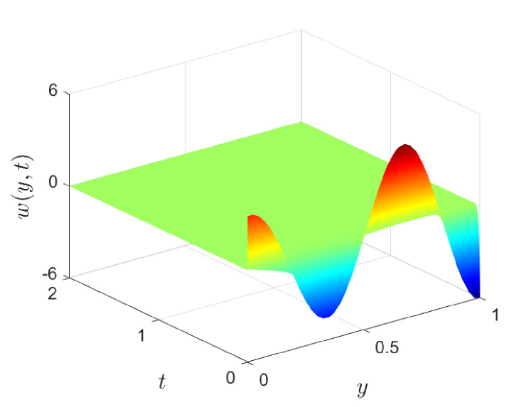
(a) Evolution of $w$ for system (14) with $A_{1}=5$ and $A_{2}=0$.

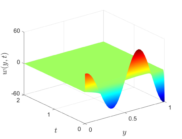
(b) Evolution of $w$ for system (14) with $A_{1}=50$ and $A_{2}=0$.

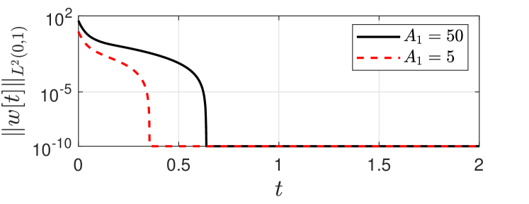
(c) Evolution of $\|w[t]\|_{L^{2}(0,1)}$ for system (14) with $A_{1}\in\{5,50\}$ and $A_{2}=0$.

Figure 1: Evolution of $w$ and $\|w[t]\|_{L^{2}(0,1)}$ for system (14) with different initial data.

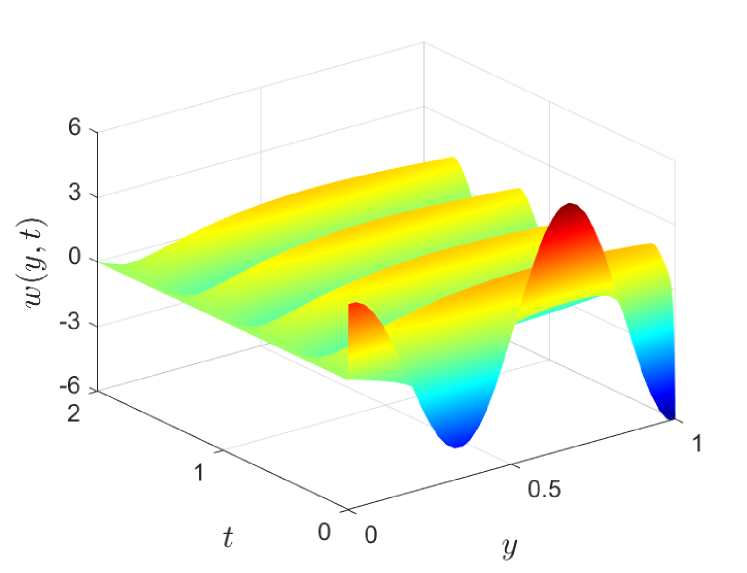
(a) Evolution of $w$ for system (14) with $A_{1}=5$ and $A_{2}=20$.

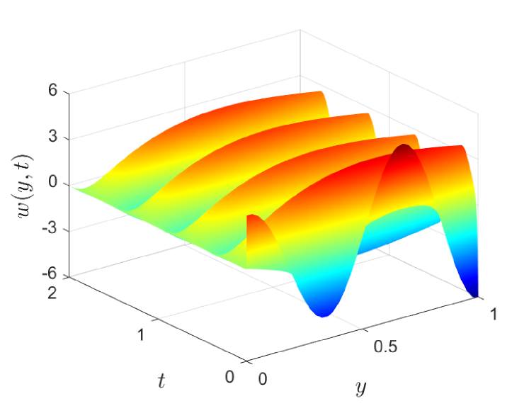
(b) Evolution of $w$ for system (14) with $A_{1}=5$ and $A_{2}=40$.

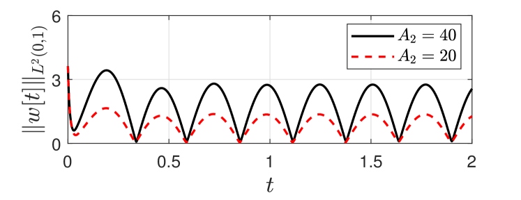
(c) Evolution of $\|w[t]\|_{L^{2}(0,1)}$ for system (14) with $A_{1}=5$ and $A_{2}\in\{20,40\}$.

Figure 2: Evolution of $w$ and $\|w[t]\|_{L^{2}(0,1)}$ for system (14) with different disturbances.

In the absence of disturbances, namely, in the case where $A_{2}=0$, Theorem 3.11 indicates that the disturbance-free system (14) is finite-time stable. This property is illustrated in Fig. 1 (a), (b), and (c). Especially, Fig. 1 (c), which is plotted in a logarithmic scale, well depicts the fast convergence property of solutions to the disturbance-free system (14) with different initial data, i.e., $A_{1}\in\{5,50\}$. In addition, it can be seen from Fig. 1 (c) that the settling time decreases when the amplitude of initial data decreases. This property is in accordance with the theoretical result described by (42).

In the presence of disturbances, namely, in the case where $A_{2}\in\{20,40\}$, for the same initial data, i.e., $A_{1}=5$, it is shown in Fig. 2 (a), (b), and (c) that the solutions of the disturbed system (14) with different disturbances remain bounded. Especially, the amplitude of solutions and their norms decreases when the amplitude of disturbances deceases. These robust properties, along with the finite-time stability property depicted by Fig. 2 (a) and (c), well illustrate the FTISS of system (14).

4 conclusion

In this paper, we extended the notion of FTISS to infinite-dimensional systems and provide Lyapunov theory-based tools to establish the FTISS of infinite-dimensional systems. In particular, we demonstrated the construction of Lyapunov functionals tailored for assessing the FTISS for a class of infinite-dimensional nonlinear systems under the framework of compact semigroup theory and Hilbert spaces, and verified the FTISS for parabolic PDEs with sublinear terms by using an interpolation inequality. Numerical results were presented to illustrate the obtained theoretical results. It is worth mentioning that designing feedback controls to achieve the FTISS for parabolic PDEs remains a challenging subject that will be considered in our future work.

References

- [1] E. D. Sontag. Smooth stabilization implies coprime factorization. IEEE Trans. Automat. Control, 34(4):435–443, 1989. http://dx.doi.org/10.1109/9.28018.
- [2] H. K. Khalil. Nonlinear Systems. Prentice-Hall, London, U. K., 1996.
- [3] A. Mironchenko. Input-to-State Stability: Theory and Application. Springer, Cham, Switzerland, 2023. https://doi.org/10.1007/978-3-031-14674-9.
- [4] E. D. Sontag and Y. Wang. On characterizations of the input-to-state stability property. Systems Control Lett., 24(5):351–359, 1995. https://doi.org/10.1016/0167-6911(94)00050-6.
- [5] E. D. Sontag and Y. Wang. New characterizations of input-to-state stability. IEEE Trans. Automat. Control, 41(9):1283–1294, 1996. http://dx.doi.org/10.1109/9.536498.
- [6] J. Park and Y. Choi. Input-to-state stability of variable impedance control for robotic manipulator. Appl. Sci., 10(4), 2020. https://doi.org/10.3390/app10041271.
- [7] Y. Wang and H. Ji. Input-to-state stability-based adaptive control for spacecraft fly-around with input saturation. IET Control Theory Appl., 14(10):1365–1374, 2020. https://doi.org/10.1049/iet-cta.2019.0634.
- [8] Y. Wang, J. Lu, J. Cao, W. Huang, J. Guo, and Y. Wei. Input-to-state stability of the road transport system via cyber-physical optimal control. Math. Comput. Simulation, 171:3–12, 2020. https://doi.org/10.1016/j.matcom.2019.05.005.
- [9] S. Dashkovskiy and A. Mironchenko. On the uniform input-to-state stability of reaction-diffusion systems. Proceedings of the 49th IEEE Conference on Decision and Control, pages 6547–6552, 2010. http://dx.doi.org/10.1109/CDC.2010.5717779.
- [10] B. Jayawardhana, H. Logemann, and E. P. Ryan. Infinite-dimensional feedback systems: the circle criterion and input-to-state stability. Commun. Inf. Syst., 8(4):413–444, 2008. https://dx.doi.org/10.4310/CIS.2008.v8.n4.a4.
- [11] H. Damak. Input-to-state stability and integral input-to-state stability of non-autonomous infinite-dimensional systems. Internat. J. Systems Sci., 52(10):2100–2113, 2021. http://dx.doi.org/10.1080/00207721.2021.1879306.
- [12] H. Damak, M. A. Hammami, and R. Heni. Input-to-state practical stability for non-autonomous nonlinear infinite-dimensional systems. Internat. J. Robust Nonlinear Control, 33:5834–5847, 2023. http://dx.doi.org/10.1002/rnc.6671.
- [13] S. Dashkovskiy and A. Mironchenko. Input-to-state stability of infinite-dimensional control systems. Math. Control Signals Systems, 25:1–35, 2013. http://dx.doi.org/10.1007/s00498-012-0090-2.
- [14] B. Jacob, R. Nabiullin, J. R. Partington, and F. L. Schwenninger. Infinite-dimensional input-to-state stability and orlicz spaces. SIAM J. Control Optim., 56(2):868–889, 2018. http://dx.doi.org/10.1137/16M1099467.
- [15] B. Jacob, A. Mironchenko, J. R. Partington, and F. Wirth. Noncoercive Lyapunov functions for input-to-state stability of infinite-dimensional systems. SIAM J. Control Optim., 58(5):2952–2978, 2020. https://doi.org/10.1137/19M1297506.
- [16] A. Mironchenko and C. Prieur. Input-to-state stability of infinite-dimensional systems: recent results and open questions. SIAM Rev., 62(3):529–614, 2020. https://doi.org/10.1137/19M1291248.
- [17] A. Mironchenko and F. Wirth. Characterizations of input-to-state stability for infinite-dimensional systems. IEEE Trans. Automat. Control, 63(6):1692–1707, 2018. http://dx.doi.org/10.1109/TAC.2017.2756341.
- [18] I. Karafyllis and M. Krstic. ISS with respect to boundary disturbances for 1-D parabolic PDEs. IEEE Trans. Automat. Control, 61(12):3712–3724, 2016. https://doi.org/10.1109/TAC.2016.2519762.
- [19] I. Karafyllis and M. Krstic. ISS in different norms for 1-D parabolic PDEs with boundary disturbances. SIAM J. Control Optim., 55(3):1716–1751, 2017. https://doi.org/10.1137/16M1073753.
- [20] I. Karafyllis and M. Krstic. Input-to-State Stability for PDEs. Springer-Verlag, Cham, 2019. https://doi.org/10.1007/978-3-319-91011-6.
- [21] H. Lhachemi and R. Shorten. ISS property with respect to boundary disturbances for a class of Riesz-spectral boundary control systems. Automatica, 109, 2019. https://doi.org/10.1016/j.automatica.2019.108504.
- [22] A. Mironchenko and H. Ito. Construction of Lyapunov functions for interconnected parabolic systems: an iISS approach. SIAM J. Control Optim., 53(6):3364–3382, 2015. https://doi.org/10.1137/14097269X.
- [23] Y. Orlov, L. Perez, O. Gomez, and L. Autrique. ISS output feedback synthesis of disturbed reaction-diffusion processes using non-collocated sampled-in-space sensing and actuation. Automatica, 122, 2020. https://doi.org/10.1016/j.automatica.2020.109257.
- [24] J. Zheng and G. Zhu. Input-to-state stability with respect to boundary disturbances for a class of semi-linear parabolic equations. Automatica, 97:271–277, 2018. https://doi.org/10.1016/j.automatica.2018.08.007.
- [25] J. Zheng and G. Zhu. A De Giorgi iteration-based approach for the establishment of ISS properties for Burgers’ equation with boundary and in-domain disturbances. IEEE Trans. Automat. Control, 64(8):3476–3483, 2019. https://doi.org/10.1109/TAC.2018.2880160.
- [26] J. Zheng and G. Zhu. Input-to-state stability for a class of one-dimensional nonlinear parabolic PDEs with nonlinear boundary conditions. SIAM J. Control Optim., 58(4):2567–2587, 2020. https://doi.org/10.1137/19M1283720.
- [27] A. Mironchenko, I. Karafyllis, and M. Krstic. Monotonicity methods for input-to-state stability of nonlinear parabolic PDEs with boundary disturbances. SIAM J. Control Optim., 57:510–532, 2019. https://doi.org/10.1137/17M1161877.
- [28] A. Smyshlyaev and M. Krstic. Closed-form boundary state feedbacks for a class of 1-D partial integro-differential equations. IEEE Trans. Automat. Control, 49(12):2185–2202, 2004. https://doi.org/10.1109/TAC.2004.838495.
- [29] J. Wang, H. Zhang, and X. Yu. Input-to-state stabilization of coupled parabolic PDEs subject to external disturbances. IMA J. Math. Control Inform., 39(1):185–218, 2022.
- [30] H. Zhang, J. Wang, and J. Gu. Exponential input-to-state stabilization of an ODE cascaded with a reaction-diffusion equation subject to disturbances. Automatica, 133, 2021. https://doi.org/10.1016/j.automatica.2021.109885.
- [31] L. Aguilar, Y. Orlov, and A. Pisano. Leader-follower synchronization and ISS analysis for a network of boundary-controlled wave PDEs. IEEE Control Syst. Lett., 5(2):683–688, 2021. https://doi.org/10.1109/LCSYS.2020.3004505.
- [32] M. S. Edalatzadeh and K. A. Morris. Stability and well-posedness of a nonlinear railway track model. IEEE Control Syst. Lett., 3(1):162–167, 2019. https://doi.org/10.1109/LCSYS.2018.2849831.
- [33] Z. Zhang, J. Zheng, and G. Zhu. Event-triggered power tracking control of heterogeneous TCL populations. IEEE Trans. Smart Grid, 15(4):3601–3612, 2024. https://doi.org/10.1109/TSG.2024.3351916.
- [34] Y. Hong, Z. Jiang, and G. Feng. Finite-time input-to-state stability and applications to finite-time control. Proceedings of the 17th IFAC Conference, 41(2):2466–2471, 2008. https://doi.org/10.3182/20080706-5-KR-1001.00416.
- [35] Y. Hong, Z. Jiang, and G. Feng. Finite-time input-to-state stability and applications to finite-time control design. SIAM J. Control Optim., 48(7):4395–4418, 2010. http://dx.doi.org/10.1137/070712043.
- [36] S. P. Bhat and D. S. Bernstein. Continuous finite-time stabilization of the translational and rotational double integrators. IEEE Trans. Automat. Control, 43(5):678–682, 1998. http://dx.doi.org/10.1109/9.668834.
- [37] J. M. Coron. On the stabilization in finite-time of locally controllable systems by means of continuous time-varying feedback law. SIAM J. Control Optim., 33(3):804–833, 1995. https://doi.org/10.1137/S0363012992240497.
- [38] Y. Hong, J. Huang, and Y. Xu. On an output feedback finite-time stabilization problem. IEEE Trans. Automat. Control, 46(2):305–309, 2001. http://dx.doi.org/10.1109/9.905699.
- [39] Y. Hong, Y. Xu, and J. Huang. Finite-time control for robot manipulators. Systems Control Lett., 46(4):243–253, 2002. https://doi.org/10.1016/S0167-6911(02)00130-5.
- [40] E. Moulay and W. Perruquetti. Finite time stability conditions for non-autonomous continuous systems. Internat. J. Control, 81(5):797–803, 2008. http://dx.doi.org/10.1080/00207170701650303.
- [41] H. Oza, Y. Orlov, and S. Spurgeon. Finite time stabilization of a perturbed double integrator with unilateral constraints. Math. Comput. Simul., 95, 2013. https://doi.org/10.1016/j.matcom.2012.02.011.
- [42] Z. Wang, S. Li, and S. Fei. Finite-time tracking control of a nonholonomicmobile robot. Asian J. Control, 11(3):344–357, 2009. https://doi.org/10.1002/asjc.112.
- [43] J. Wang, H. Liang, Z. Sun, S. Zhang, and M. Liu. Finite-time control for spacecraft formation with dual-number-based description. J. Guidance Control Dynam., 35(3):950–962, 2012. https://dx-doi-org-s.era.lib.swjtu.edu.cn/10.2514/1.54277.
- [44] F. Lopez-Ramirez, D. Efimov, A. Polyakov, and W. Perruquetti. On implicit finite-time and fixed-time ISS Lyapunov functions. Proceedings of the 57th Conference on Decision and Control, 2018. https://inria.hal.science/HAL-01888526.
- [45] F. Lopez-Ramirez, D. Efimov, A. Polyakov, and W. Perruquetti. Finite-time and fixed-time input-to-state stability: explicit and implicit approaches. Systems Control Lett., 144, 2020. http://dx.doi.org/10.1016/j.sysconle.2020.104775.
- [46] A. Aleksandrov, D. Efimov, and S. Dashkovskiy. Design of finite-/fixed-time ISS-Lyapunov functions for mechanical systems. Math. Control Signals Systems, pages 1–21, 2022.
- [47] S. Liang and J. Liang. Finite-time input-to-state stability of nonlinear systems: the discrete-time case. Internat. J. Systems Sci., 54(3):583–593, 2023. https://doi.org/10.1080/00207721.2022.2135418.
- [48] G. Li, M. Xin, and C. Miao. Finite-time input-to-state stability guidance law. J. Guidance Control Dynam., 41(10):2199–2213, 2018. https://doi.org/10.2514/1.G003519.
- [49] Z. Zhang, J. Zheng, and G. Zhu. Power tracking control of heterogeneous populations of thermostatically controlled loads with partially measured states. IEEE Access, 12:57674–57687, 2024. https://doi.org/10.1109/ACCESS.2024.3392511.
- [50] X. Sun, J. Zheng, and G. Zhu. Prescribed-time input-to-state stability of infinite-dimensional systems. Proceedings of the 39th Youth Academic Annual Conference of Chinese Association of Automation (YAC), pages 1900–1905, 2024. https://doi.org/10.1109/YAC63405.2024.10598638.
- [51] Y. Song, Y. Wang, J. Holloway, and M. Krstic. Time-varying feedback for regulation of normal-form nonlinear systems in prescribed finite time. Automatica, 83:243–251, 2017. http://dx.doi.org/10.1016/j.automatica.2017.06.008.
- [52] A. Mironchenko. Small gain theorems for general networks of heterogeneous infinite-dimensional systems. SIAM J. Control Optim., 59(2):1393–1419, 2021. https://doi.org/10.1137/19M1238502.
- [53] A. Pazy. Semigroups of Linear Operators and Applications to Partial Differential Equations. Springer-Verlag, New York, 1983. http://dx.doi.org/10.1007/978-1-4612-5561-1.
- [54] L. C. Evans. Partial Differential Equations. American Mathematical Society, Providence, Rhode Island, 2010. https://www.lib.swjtu.edu.cn/asset/detail/10159686968.