Dipole representation of composite fermions in graphene’s quantum Hall systems

Abstract

The even denominator fractional quantum Hall effect has been experimentally observed in the fourth Landau level ($n=3$). This paper is motivated by recent studies regarding the possibility of pairing and the nature of the ground state in this system. By extending the dipole representation of composite fermions, we adapt this framework to the context of graphene’s quantum Hall systems, with a focus on half-filled Landau levels. We derive an effective Hamiltonian that incorporates the key symmetry of half-filled Landau levels, particularly particle-hole symmetry. At the Fermi level, the energetic instability of the dipole state is influenced by the interplay between topology and symmetry, driving the system towards a critical state. We explore the possibility that this critical state stabilizes into one of the paired states with well-defined pairing solutions. However, our results demonstrate that the regularized state which satisfies boost invariance at Fermi level and lacks well- defined pairing instabilities emerges as energetically more favorable. Therefore, we find no well- defined pairing instabilities of composite fermions in the dipole representation in the half-filled fourth Landau level ($n=3$) of electrons in graphene. Although the theory of composite fermions has its limitations, further research is required to investigate other possible configurations. We discuss the consistency of our results with experimental and numerical studies, and their relevance for future research efforts.

I Introduction

The discovery of the fractional quantum Hall effect (FQHE) [1] represents a significant breakthrough in the study of topological states of matter, introducing a rich landscape of quantum phases driven by electron correlations in two-dimensional electron systems (2DES) [2]. Among the most intriguing manifestations of the FQHE is the observation of a quantized Hall plateau at the filling factor $\nu=5/2$ [3], indicating the FQHE at the half-filled second Landau level ($n=1$). The observation of even-denominator FQHE states is astonishing, considering that the fermionic statistics of electrons suggest the denominator of the fraction should be an odd number. These significant discoveries have inspired intensive theoretical and experimental efforts to decode the underlying physics and implications of these states.

The concept of composite fermions (CFs), introduced by Jain [4, 5], has provided an insightful framework for comprehending various aspects of quantum Hall phenomena, primarily for the half-filled second LL ($n=1$). CFs are quasiparticles formed by attaching an even number of quantized vortices to electrons.

In recent years, advancements in noncommutative field theory in high-energy physics, have inspired Dong and Senthil [6] to revisit longstanding problems in quantum Hall physics. In particular, this includes the problem of the LL at $\nu=1$ for bosons, initially formulated by Pasquier and Haldane [7], and further developed by Read [8]. This problem involves an additional degree of freedom, namely the vortex degree of freedom, where each boson is associated with a single flux of the magnetic field, and since vortices are fermionic, and the resulting composite quasiparticles are neutral, resembles CFs. Furthermore, CFs experience a zero average effective magnetic field, similar to electrons at $\nu=1/2$. Unlike previous approaches that relied on an averaged field energy, Dong and Senthil [6] introduced the concept of intrinsic dipole energy. The application of noncommutative field theory to quantum Hall systems has since led to significant advancements, with recent studies extending these concepts to various quantum Hall states [9, 10, 11, 12, 13, 14].

Recently, FQH states with additional half-integer values have been observed in various materials, such as graphene, a monolayer of carbon atoms arranged in a hexagonal lattice. Graphene’s unique electronic and topological properties make it a promising candidate for studying exotic quantum phenomena, including FQHE. Namely, recent experimental study by Kim et al. [15], has identified FQHE states at half-filling in the fourth LL ($n=3$) of monolayer graphene. Additionally, research by [16], has explored CF pairing in monolayer graphene using alternative pairing functions and numerical modeling of a system on a torus. They concluded that using the Bardeen-Cooper-Schrieffer (BCS) variational state [17] for CFs reveals an $f$- wave pairing instability for the interaction characteristic of the $n=3$ LL without any modification of Coulomb potential. Additionally, they suggested the possibility of a $p$-wave instability for the $n=2$ LL, where FQHE has not been experimentally observed. However, these findings are in contrast with numerical studies on the sphere, which have not observed such pairing instabilities [15]. The disparity between these results highlights the need for further investigation. Besides, topological pairing, particularly $p$-wave and $f$-wave, is crucial for quantum computing applications due to its non-Abelian statistics, which enable robust qubits and fault-tolerant quantum operations [18].

The dipole representation of FQHE states, introduced in Ref. [13], is particularly relevant to this study. In this representation, dipoles are neutral composite objects formed by an electron and its correlation hole. These dipoles possess moments proportional to their momentum in an external magnetic field. This effective theory has proven to be robust, capturing the microscopic description of several problems and aligning with previous experimental and numerical studies. In particular, it yielded results consistent with numerical and experimental studies of 2DES, where the Pomeranchuk instability is observed in higher half-filled LLs. A recent study [19] even provided an explanation for the mechanism of $p$-wave pairing of CFs at half-filling in the second LL ($n=1$) of electrons in 2DES and in the fully filled first LL ($n=0$) of bosons, further underscoring the importance of this representation.

In this paper, we aim to explore the potential for CF pairing in monolayer graphene using the BCS framework, also utilizing the dipole representation. The half-filled LL system possesses an additional feature, the particle-hole (PH) symmetry [13], which implies that the density of holes corresponds to the density of composite holes. Consequently, this state is energetically unstable with respect to repulsive interactions, leading to a critical state. Through analytical studies, we demonstrate that in the fourth LL $(n=3)$ of a graphene monolayer, this critical state is not stabilized by selecting one of the two possible symmetry-broken paired states; instead, it stabilizes into a regularized non-paired state, which cannot support gapped pairing solutions due to the absence of mass. Our findings are consistent with numerical studies conducted on spherical geometries [15].

This paper is organized as follows: In Section II, we introduce the necessary formalism and key concepts of the dipole representation and apply them to the half-filled LLs of electrons in graphene. In particular, we discuss the model, and the effective Hamiltonian in the dipole representation. Section III explores the possibility and mechanism of paired states within the context of the dipole representation and analyzes their stability. Finally, in Section IV, we conclude with a discussion of our findings and their implications for future research.

II Implementing Boost Invariance and State Regularization in Graphene’s Landau Levels

II.1 The model

Graphene exhibits unique electronic properties, including a ”relativistic” quantum Hall effect due to its charge carriers, which behave as massless Dirac fermions [20, 21]. In graphene, electrons are arranged in a honeycomb lattice composed of two sublattices, $A$ and $B$, and their behavior can be described by a two-dimensional Dirac equation [22]. In a tight-binding model, we consider only the nearest neighbor hopping parameter $t$ between sites $A$ and $B$. The low energy properties of graphene are captured by a two-band model labeled as $\lambda=\pm$ where the dispersion is linear. The valence band $\lambda=+$ and the conduction band $\lambda=-$ touch each other at the two inequivalent corners $K_{+}$ and $K_{-}$ (referred to as valleys) of the Brillouin zone [22, 23].

When an external magnetic field is applied, the Hamiltonian for low-energy states around the $K_{+}$ valley is given by [24, 25]:

$$H=v\begin{pmatrix}0&\pi^{\dagger}\\ \pi&0.\end{pmatrix}$$ (1)

where $v=\frac{\sqrt{3}}{2}\frac{at}{\hbar}$ is the velocity, and the operators $\pi^{\dagger}$ and $\pi$, in the Landau gauge, coincide with the LL creation and annihilation operators, respectively [25].

Here, we focus on spinless electrons confined to the $n$-th LL, where only intra-LL excitations are considered.

The spinor states in the $\lambda-$band, obtained from the two-dimensional Dirac equation, can be expressed as:

$$\psi_{\lambda n,m}^{\xi}=\frac{1}{\sqrt{2}}\begin{pmatrix}|\,n-1,\,m\,\rangle\\ \lambda|\,n,\,m\,\rangle\end{pmatrix},$$ (2)

for $n\neq 0$

$$\psi_{n=0,m}^{\xi}=\begin{pmatrix}0\\ |0,\,m\,\rangle\end{pmatrix},$$ (3)

for $n=0$, in terms of the harmonic oscillator states $\left|\,n,\,m\,\right\rangle$ and the guiding-center quantum number $m$. These spinors describe states within the $n$-th LL in the band $\lambda$. The first component of the spinor represents the amplitude on the $A$ sublattice at the point $K_{+}$ ($\xi=+$) and the amplitude on the $B$ sublattice at the point $K_{-}$ ($\xi=-$).

II.2 The Pasquier-Haldane-Read construction for half-filled LL of electrons in graphene

In this section, we extend the traditional Pasquier-Haldane-Read (PHR) construction [7, 8] to describe the complex excitations in half-filled LLs of electrons in graphene. Unlike the original model, which was formulated for fully filled LLs of bosons, our approach adapts the PHR construction to systems where LLs are half-filled of electrons. In this paper, we employ an expansion of the Hilbert space by incorporating correlation holes, which are positive charges that pair with electrons to form neutral dipoles. This representation is crucial for describing systems with PH symmetry, a key characteristic of half-filled LLs, and for maintaining the topological properties of the quantum Hall states.

We begin by representing the basis states in a LL as:

$$\{|o_{1}\rangle,|o_{2}\rangle,\ldots,|o_{N_{\phi}/2}\rangle,|m_{1}\rangle,|m_{2}\rangle,\ldots,|m_{N_{\phi}/2}\rangle\},$$ (4)

where $|o_{i}\rangle$ and $|m_{i}\rangle$ represent the states in the physical and orthogonal subspaces, respectively. These states form the foundation for describing the system in our enlarged Hilbert space, which accommodates both electrons and correlation holes [13]. Here, $N_{\phi}$ represents the number of orbitals.

In this expanded space, we define creation and annihilation operators that satisfy the algebra:

$$\{c_{mo},c_{o^{\prime}m^{\prime}}^{\dagger}\}=\delta_{mm^{\prime}}\delta_{oo^{\prime}},$$

$$\{c_{mo},c_{o^{\prime}m^{\prime}}\}=0,$$

$$\{c_{mo}^{\dagger},c_{o^{\prime}m^{\prime}}^{\dagger}\}=0.$$ (5)

These operators $c_{mo}$ and $c^{\dagger}_{mo}$ in the LL have double indices. Using these operators, we define the Fourier components of the physical (left) and unphysical (right) densities in the n-th LL, incorporating the form factor $F_{n}(|\vec{q}|)$ :

$$\rho_{n}^{L}(\vec{q})=F_{n}(|\vec{q}|)\sum_{o,\,o^{\prime}}\sum_{m}\langle o|\tau_{-\vec{q}}|o^{\prime}\rangle c_{mo}^{\dagger}c_{o^{\prime}m},$$ (6)

$$\rho_{n}^{R}(\vec{q})=F_{n}(|\vec{q}|)\sum_{m,\,m^{\prime}}\sum_{o}\langle m|\tau_{-\vec{q}}|m^{\prime}\rangle c_{mo}^{\dagger}c_{om^{\prime}}.$$ (7)

Here, $\tau_{\vec{q}}=e^{i\vec{q}\vec{R}}$ is the translation operator, where $\vec{R}=\left(X,Y\right)$ represents the guiding center coordinates of a CF [26, 27, 28] in the external magnetic field $\vec{B}=-B\vec{e}_{z}$, with components obeying the commutation relation:

$$\left[X,Y\right]=il_{B}^{2}.$$ (8)

Here, $l_{B}$ is the magnetic length. In what follows, we will set $l_{B}\equiv 1$. This framework ensures that the neutral CFs are accurately described within the context of the LL dynamics.

The Fourier components of the form factor in the n-th LL are given in terms of Laguerre polynomials in the following way:

$$F^{(n)}(q)=\begin{cases}1&\text{if }n=0,\\ \frac{1}{2}\left[L_{n-1}\left(\frac{q^{2}}{2}\right)+L_{n}\left(\frac{q^{2}}{2}\right)\right]&\text{if }n\neq 0.\end{cases}$$ (9)

For $n=0$, the form factor for graphene coincides with that of a 2DES, such as GaAs. However, for higher $n$ it can be viewed as an average of the two form factors of those for 2DES [29].

Furthermore, the annihilation operator can be written in relation to its momentum space representation in the following way:

$$c_{mo}=\int\frac{d\vec{k}}{(2\pi)^{2}}\langle m|\tau_{\vec{k}}|o\rangle c_{\vec{k}}.$$ (10)

By substituting Eq. (10) into the equations for the left and right density operators, Eq. (6) and Eq. (7), we obtain:

$$\rho_{n}^{L}(\vec{q})=F_{n}(\vec{q})\int\frac{d^{2}\vec{k}}{(2\pi)^{2}}e^{\frac{i}{2}\vec{k}\times\vec{q}}c_{\vec{k}-\vec{q}}^{\dagger}c_{\vec{k}},$$ (11)

$$\rho_{n}^{R}(\vec{q})=F_{n}(\vec{q})\int\frac{d^{2}\vec{k}}{(2\pi)^{2}}e^{-\frac{i}{2}\vec{k}\times\vec{q}}c_{\vec{k}-\vec{q}}^{\dagger}c_{\vec{k}}.$$ (12)

Using the relations Eq. (5), it is easy to show that these densities obey the Girvin-MacDonald-Platzman (GMP) algebra [31]:

$$\left[\rho_{0}^{L}(\vec{q}),\rho_{0}^{L}(\vec{q}^{\prime})\right]=2i\sin\left(\frac{\vec{q}\times\vec{q}^{\prime}}{2}\right)\rho_{0}^{L}(\vec{q}+\vec{q}^{\prime}),$$

$$\left[\rho^{R}_{0}(\vec{q}),\rho^{R}_{0}(\vec{q}^{\prime})\right]=-2i\sin\left(\frac{\vec{q}\times\vec{q}^{\prime}}{2}\right)\rho_{0}^{R}(\vec{q}+\vec{q}^{\prime}),$$

$$\left[\rho^{L}_{0}(\vec{q}),\rho_{0}^{R}(\vec{q}^{\prime})\right]=0.$$ (13)

This is induced by the commutation relation Eq. (8), and restriction to the single LL. The realization of the GMP algebra using the canonical CF variables facilitates the application of mean-field methods [8].

II.3 The effective Hamiltonian in dipole represenation in graphene

To accurately describe the system within the dipole representation, it is essential to impose a specific constraint. These constraints serve several purposes. First, the constraint ensures that the number of degrees of freedom in the effective model aligns with the microscopic description of the physical problem. Furthermore, the constraint also defines the physical subspace within the enlarged Hilbert space, which includes additional degrees of freedom such as correlation holes. Second, the imposed constraint must preserve the PH symmetry, a fundamental characteristic of the half-filled LL, ensuring that the model accurately reflects the physical properties of the system.

We introduce the following constraint:

$$\rho_{nn}^{L}+\rho_{nn}^{R}=1$$ (14)

This constraint acts as a null operator in momentum space:

$$\rho_{\vec{q}}^{L}+\rho_{\vec{q}}^{R}=0.$$ (15)

It is important to note that this constraint involves both physical and unphysical quantities, treating them as interdependent. Since the right degrees of freedom (additional degrees of freedom) represent correlation holes in the enlarged space, this constraint effectively ensures, in the long-distance limit, that the density of correlation holes equals the density of real holes.

Furthermore, when defining the problem in the enlarged space, operators, including the Hamiltonian, may map physical states into superpositions of physical and unphysical states. To ensure that physical states remain within the physical subspace, the Hamiltonian must commute with the constraint.

The effective Hamiltonian in this framework must reflect the dipole representation within $n$-th LL. Additionally, it must preserve PH symmetry, meaning it remains invariant under the exchange of particles and holes. The Hamiltonian is carefully constructed to satisfy these conditions, and we impose a constraint that ensures the resulting Hamiltonian has a PH symmetric form:

$$\mathcal{H}_{\text{eff}}=\frac{1}{8}\int\frac{d^{2}\vec{q}}{(2\pi)^{2}}V^{(n)}(\vec{q})\left(\rho_{L}(\vec{q})-\rho_{R}(\vec{q})\right)\left(\rho_{L}(-\vec{q})-\rho_{R}(-\vec{q})\right).$$ (16)

Here, $V^{(n)}(\vec{q})=\frac{1}{|q|}e^{-q^{2}/2}$ represents the Fourier transformed Coulomb potential, which takes into account states within the n-th LL. The form factor mimics the LL characteristics.

Using mean-field approximation and Hartree-Fock (HF) calculations, one easily finds that dispersion relation for graphene for the n-th LL has the following form:

$$\varepsilon(\vec{k})=\varepsilon_{0}(\vec{k})+\varepsilon_{I}(\vec{k}),$$ (17)

where:

$$\varepsilon_{0}^{(n)}(\vec{k})=\frac{1}{2}\int\frac{d^{2}\vec{q}}{(2\pi)^{2}}V^{(n)}(|\vec{q}|)\sin^{2}\left(\frac{\vec{k}\times\vec{q}}{2}\right),$$ (18)

represents single-particle energy and

$$\varepsilon_{HF}^{(n)}(\vec{k})=-\int\frac{d^{2}\vec{q}}{(2\pi)^{2}}V^{(n)}(|\vec{k}-\vec{q}|)\sin^{2}\left(\frac{\vec{k}\times\vec{q}}{2}\right)n_{q},$$ (19)

represents the HF contributions. Here, $n_{q}$ is the Fermi (step) function with $n_{q}=1$ for $q$ inside a circular Fermi surface of radius $q_{F}$, and zero otherwise. This results aligns with [32], with the difference that here $V(|\vec{q}|)$ represents the Coulomb interaction in the graphene system in the n-th LL, and includes an additional factor of $1/4$ that reduces the strength of the Coulomb interaction. Furthermore, the single particle energy $\varepsilon_{0}^{(n)}$ can be obtained in a closed analytical fashion as detailed in Appendix A. Moreover, in Appendix A we also give the complete data of the corresponding energies for the lowest fourth LL ($n=0,1,2,3$). On the other hand, we obtained the energy of interaction of this particles $\varepsilon_{HF}^{(n)}$ via numerical integration.

II.4 Boost Invariance and State Regularization in Graphene

In this section, we derive the Hamiltonian from the constraint previously established, ensuring that our effective theory maintains a valid microscopic description, at least at the Fermi level. The Hamiltonian described in Eq. (16), which governs the dipole representation, incorporates a finite (bare) mass for single-particle energies as a consequence of the dipole structure. To achieve this, it is essential that the Hamiltonian exhibit boost invariance, which imposes a condition on the (bare) mass at the Fermi level.

To begin, we introduce an interaction term that is null within the physical space:

$$\mathcal{H}_{0}=\mathcal{C}_{n}\int\frac{d^{2}\vec{q}}{(2\pi)^{2}}V^{(n)}(\vec{q})\left(\rho_{L}(\vec{q})+\rho_{R}(\vec{q})\right)\left(\rho_{L}(-\vec{q})+\rho_{R}(-\vec{q})\right).$$ (20)

Therefore, the resulting Hamiltonian has the following form:

$$\mathcal{H}_{\text{res}}=\mathcal{H}_{\text{eff}}+\mathcal{H}_{\text{0}}.$$ (21)

Furthermore, we denote the constant $\mathcal{C}_{n}$ such that the energy $\varepsilon_{1}$ denoting the single energy of the resulting Hamiltonian in Eq. (21) fulfills the condition:

$$\frac{1}{m^{*}}=\frac{\partial^{2}\varepsilon_{\text{1}}(\vec{k})}{\partial k^{2}}\Big{|}_{k=k_{F}}=0,$$ (22)

where $m^{*}$ is the effective mass. Therefore, the resulting Hamiltonian in Eq. (21) has no terms $\frac{k^{2}}{m^{*}}$, which contribute to the kinetic energy.

III Dipole representation of composite fermions in graphene

As discussed earlier, a key feature of the Hamiltonian in the dipole representation of CFs is its inherent symmetry, particularly PH symmetry. This symmetry means that the system remains unchanged when particles are exchanged with real holes or when the densities $\rho_{L}(\vec{q})$ and $\rho_{R}(\vec{q})$ are swapped, where $\rho_{R}(\vec{q})$ corresponds to the density of correlation holes.

In the context of the Coulomb interaction, it is energetically favorable for these correlation holes to move away from the electrons, allowing real holes to surround the electrons instead. We have previously shown that the density of these correlation holes is equal to the density of real holes, and that the size of the resulting dipoles is determined by a translation operator. As a result, at the Fermi level $k=k_{F}$, the electrons are positioned far from the holes, making this state energetically unstable and prone to becoming critical.

In this scenario, breaking the symmetry between the left (L) and right (R) components of the system is equivalent to breaking the symmetry between particles and real holes. Therefore, states that break this symmetry are likely to be more energetically stable.

Motivated by the aim to explore a well-defined state of CFs within the dipole representation, that stabilizes the critical state, we derive an effective Hamiltonian. This is achieved by revisiting the Hamiltonian in Eq. (16) and subsequently subtracting (or adding) the following term:

$$\mathcal{H}_{1}=\frac{1}{8}\int\frac{d^{2}\vec{q}}{(2\pi)^{2}}V^{(n)}(\vec{q})\left(\rho_{R}(-\vec{q})+\rho_{L}(-\vec{q})\right)\left(\rho_{R}(\vec{q})-\rho_{L}(\vec{q})\right).$$ (23)

which effectively represents zero in the physical space. Consequently, the resulting effective Hamiltonians take the following forms:

$$\mathcal{H}_{\text{res}}^{(1)}=\frac{1}{4}\int\frac{d^{2}\vec{q}}{(2\pi)^{2}}V^{(n)}(\vec{q})\rho_{R}(-\vec{q})\left(\rho_{R}(\vec{q})-\rho_{L}(\vec{q})\right),$$ (24)

and

$$\mathcal{H}_{\text{res}}^{(2)}=\frac{1}{4}\int\frac{d^{2}\vec{q}}{(2\pi)^{2}}V^{(n)}(\vec{q})\rho_{L}(-\vec{q})\left(\rho_{L}(\vec{q})-\rho_{R}(\vec{q})\right).$$ (25)

The dipole representation of these Hamiltonians plays a crucial role in defining a single energy, which is essential for obtaining paired solutions. Additionally, they can also be interpreted as symmetry-breaking modifications of the Hamiltonian in Eq. (16), stabilizing the system into one of two paired states.

To explore potential paired solutions, we apply the HF approach to the relevant part of the Hamiltonian in Eq. (24), yielding:

$$\mathcal{H}_{HF}^{(n)} =\int\frac{d^{2}\vec{k}}{(2\pi)^{2}}\,\xi_{n}(\vec{k})\,c_{\vec{k}}^{\dagger}c_{\vec{k}}\,+$$

$$+\frac{1}{4}\int\frac{d^{2}\vec{q}}{(2\pi)^{2}}\int\frac{d^{2}\vec{k_{1}}}{(2\pi)^{2}}\int\frac{d^{2}\vec{k_{2}}}{(2\pi)^{2}}V(|\vec{q}|)F_{n}^{2}(|\vec{q}|)\left(1-e^{i\vec{k}\times\vec{q}}\right)$$

$$\cdot\left(\langle c_{\vec{k}_{1}+\vec{q}}^{\dagger}c_{\vec{k}_{2}-\vec{q}}^{\dagger}\,\rangle\,c_{\vec{k}_{1}}c_{\vec{k}_{2}}+c_{\vec{k}_{1}+\vec{q}}^{\dagger}c_{\vec{k}_{2}-\vec{q}}^{\dagger}\,\langle c_{\vec{k}_{1}}c_{\vec{k}_{2}}\rangle-\right.$$

$$-\left.\langle c_{\vec{k}_{1}+\vec{q}}^{\dagger}c_{\vec{k}_{2}-\vec{q}}^{\dagger}\,\rangle\,\langle c_{\vec{k}_{1}}c_{\vec{k}_{2}}\rangle\right),$$ (26)

where $\xi_{n}(\vec{k})=\varepsilon_{n}(\vec{k})-\varepsilon_{n}(\vec{k}_{F})$, with $\epsilon_{n}(\vec{k})$ representing the dispersion relation given by:

$$\varepsilon_{n}(\vec{k}) =\frac{1}{4}\int\frac{d^{2}\vec{q}}{(2\,\pi)^{2}}V(|\vec{q}|)F_{n}^{2}(|\vec{q}|)\left(1-e^{i\vec{k}\times\vec{q}}\right)$$

$$-\frac{1}{2}\int\frac{d^{2}\vec{q}}{(2\,\pi)^{2}}V(|\vec{k}-\vec{q}|)F_{n}^{2}(|\vec{k}-\vec{q}|)\left(1-e^{i\vec{k}\times\vec{q}}\right).$$ (27)

Furthermore, we define:

$$\Delta_{n}(\vec{k})= -\frac{1}{4}\int\frac{d^{2}\vec{q}}{(2\pi)^{2}}V(|\vec{k}-\vec{q}|)F_{n}^{2}(|\vec{k}-\vec{q}|)\left(1-e^{-i\vec{k}\times\vec{q}}\right)$$

$$\cdot\langle c_{\vec{k}_{1}}c_{\vec{k}_{2}}\,\rangle$$ (28)

Finally, using standard BCS transformations to diagonalize the Hamiltonian in Eq. (24), we obtain the total energy:

$$E_{\text{TOT}}^{(n)}=\int\frac{d^{2}\vec{k}}{(2\,\pi)^{2}}\left(\xi_{n}(\vec{k})-E_{n}(\vec{k})\right)+\int\frac{d^{2}\vec{k}}{(2\,\pi)^{2}}\frac{|\Delta_{n}(\vec{k})|^{2}}{2E_{n}(\vec{k})},$$ (29)

where the Bogoliubov quasiparticle energy is given by $E_{n}(\vec{k})=\sqrt{\xi_{n}^{2}(\vec{k})+|\Delta_{n}(\vec{k})|^{2}}$. In the BCS treatment, we obtain the pairing instability is described by the order parameter $\Delta(\vec{k})$ by self-consistently:

$$|\Delta_{n}^{(l)}(\vec{k})|=\frac{1}{4}\int\frac{d^{2}\vec{q}}{(2\pi)^{2}}V(|\vec{k}-\vec{q}|)F_{n}^{2}(|\vec{k}-\vec{q}|)\left(1-e^{-i\vec{k}\times\vec{q}}\right)\frac{\Delta_{n}^{(l)}(\vec{q})}{2E_{n}(\vec{q})}.$$ (30)

Here, the gap function takes the following form: $\Delta^{(l)}(\vec{k})=e^{il\theta_{l}}|\Delta(\vec{k})|$, where $\theta$ is the angular coordinate of $k$, with $l=0,\pm 1,\pm 2,\pm 3$ representing different pairing channels. Details regarding the numerical solutions of the self-consistent equation in Eq. (30) are provided in the Appendix B. Initially, we find the self-consistent solution given by Eq. (30), which corresponds to the minimum of the total energy. We note that we obtain the same solutions for $l=1$ in Hamiltonian Eq. (25) as we do for $l=-1$ in Hamiltonian Eq. (24).

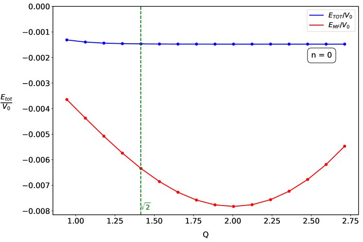
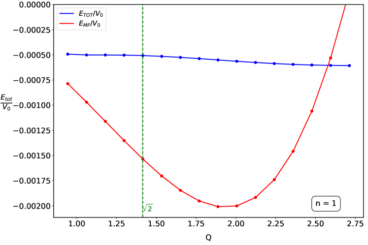
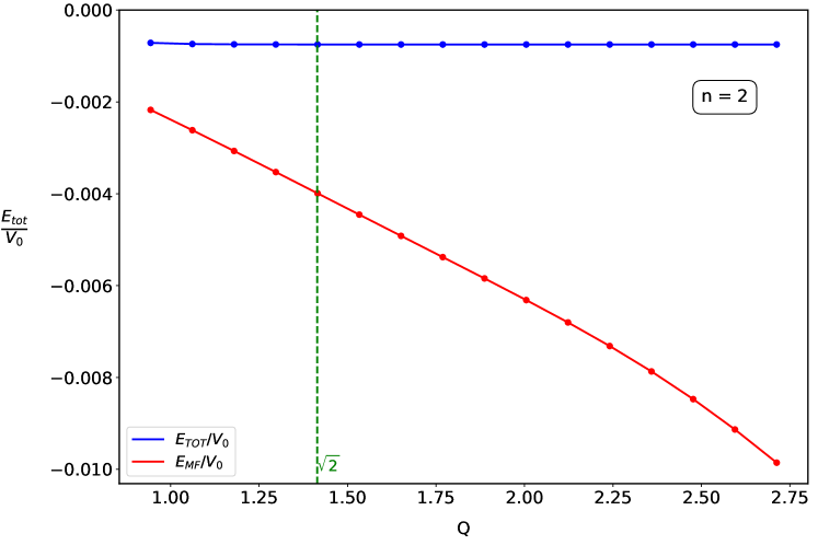
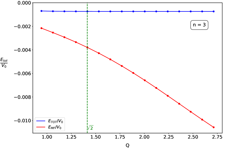
Figure 1: Total energies of the pairing solutions $E_{\text{TOT}}$ and the regularized state $E_{\text{MF}}$ in the four lowest LLs ($n=0,1,2,3$), across an interval of cut-off values $Q$. The interaction strength is characterized by $V_{0}=4\pi e^{2}/l_{B}$

In the previous section, we regularized the state of the Hamiltonian in Eq. (21) by eliminating the quadratic term, which contributes to the kinetic energy. Consequently, the regularized state cannot support gapped pairing solutions due to the absence of (bare) mass. While the critical state can be stabilized among the paired states, it can also be stabilized within the regularized state. To investigate in which of these states the critical state is stabilized, we define the energy of the regularized state of CFs in the dipole representation using a mean-field approach as follows:

$$E_{\text{MF}}=\int\frac{d^{2}\vec{k}}{(2\pi)^{2}}\left(\varepsilon_{\text{0}}(\vec{k})+\frac{1}{2}\varepsilon_{\text{HF}}(\vec{k})\right).$$ (31)

In calculating the total energy, we apply a ”cut-off” when necessary, using the radius of a circle in momentum space $Q=\sqrt{2}\,k_{F}$, which denotes the volume of available states in the LL. We also investigate how different cut-offs affect the system’s topology and pairing instability. The kinetic energy depends on the cut-off: the larger cut-off results in higher the kinetic energy, which in turn influences the stability of paired states. Furthermore, the energy of the regularized state is particulary sensitive to the cut-off (Fig. (1)), with the only viable cut-off value for this state being $k_{F}$, as it is designed to accurately describe the physics at the Fermi surface $k_{F}$. In spherical coordinates, this corresponds to $Q=\sqrt{2}\,k_{F}$.

In Fig. (1), we compare the results for $E_{MF}$ and $E_{TOT}$ in the case of graphene over an interval of cut-off values $Q$ for the four lowest LLs ($n=0,1,2,3$) to investigate the possibility of pairing instability. We find that the critical state is stabilized within the regularized state, which is energetically more favorable than the paired states. In the following sections, we will discuss these findings in more detail for each of the four lowest LLs ($n=0,1,2,3$), emphasizing how our results align with previous experiments and numerical studies.

In the lowest LL ($n=0$), considering the short-range, repulsive Coulomb interaction $V(|\vec{q}|)=q^{2}e^{-q^{2}/2}$, which describes a two-body interaction between dipoles, the three-body Hamiltonian can be derived using the Chern-Simons approach [36, 37] as follows:

$$\mathcal{H}_{\text{eff}}^{(e)}=\sum_{\langle ijk\rangle}\nabla^{2}_{i}\delta^{2}(\vec{x}_{i}-\vec{x}_{j})\delta^{2}(\vec{x}_{i}-\vec{x}_{k}),$$ (32)

which aligns with the commonly used interaction model for the Pfaffian [38]. In the lowest LL ($n=0$), the effective interaction between CFs (and therefore the physics in general) in monolayer graphene is the same as in a 2DES, such as GaAs quantum wells with zero width. Here, numerical experiments indicate that the Fermi-liquid-like state is the most stable in the half- filled first LL ($n=0$).

In the half-filled second LL ($n=1$), non-trivial topology is identified via Majorana edge states in the case of 2DES. In this LL, well-defined $p$-wave solutions in 2DES are present, particularly $l=1$ ($l=-1$) wave pairing in Hamiltonian as described in Eq. (25) (Eq. (24)), but with form factors characteristic of 2DES [19]. This corresponds to the Pfaffian topological order [38]. The PH conjugate of the Pfaffian, the anti-Pfaffian, can be obtained by switching the sign of the particles [39, 40]. We would like to point out here that a well- defined paired state can only exist if the effective dipole physics at the Fermi level, driven by the non-trivial topology of the LL, is present. However, in monolayer graphene, the regularized state dominates over the paired state, which is consistent with earlier studies indicating that the lowest energy state is a Fermi sea of CFs with no pairing instabilities [41].

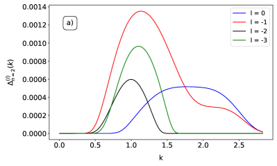
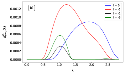
Figure 2: The solutions for $\Delta(\vec{k})$ calculated self-consistently using Eq. (30) for different pairing channels $l$: (a) in the third LL ($n=2$) and (b) in the fourth LL ($n=3$).

In the half-filled third LL ($n=2$) of graphene, the FQHE has not been observed [42, 43]. However, in numerical experiments on a torus using a BCS variational state for CFs, the authors in Ref. [17] identified the presence of pairing instability, which most likely corresponds to $p$-wave pairing. This raises the possibility that pairing may have been detected in numerical simulations, even though neither FQHE nor pairing have been observed in experiments. On the other hand, we illustrate in Fig. (2) the self-consistently obtained mean-field parameter $\Delta(\vec{k})$ in this LL. This may result in the observation of pairing solutions in the thermodynamic limit, which is well represented in numerical experiments on a torus. In contrast with this numerical study constructed on torus, we propose that the regularized state is energetically more favorable, which does not exhibit well-defined pairing solutions.

Finally, in previously mentioned study [17], it has been proposed that the Fermi sea of CFs may be unstable to $f$-wave pairing in the half-filled fourth LL ($n=3$) of graphene. The self-consistently obtained mean-field parameter in this LL is visualized in Fig. (2). This particular LL is significant due to the experimental observation of the FQHE [15]. However, numerical studies conducted on a spherical geometry reveal that neither the anti-Pfaffian nor the PH symmetric Pfaffian [44] states exhibit a strong overlap with the exact ground state near the pure Coulomb interaction point. Additionally, various spin and valley singlet states were examined, yet none showed significant overlap with the ground state in the $n=3$ LL. Although the 221-parton state [45] demonstrates a notable similarity to the pure Coulomb interaction across a wide parameter range, its validation still requires further theoretical and experimental studies. Our findings suggest that the critical state in the fourth LL ($n=3$) is not stabilized among the paired states, such as the Pfaffian. Instead, the regularized state, which lacks well-defined pairing instabilities, emerges as energetically more favorable. This suggests the absence of well-defined pairing instabilities within the dipole representation of CFs in this context. Therefore, our results are consistent with numerical studies conducted on spherical geometry. To conclusively validate the nature of the ground state and fully elucidate the pairing mechanism, particularly in higher LLs, additional theoretical and experimental research extending beyond the framework of CFs is essential. Strong short-range repulsive interaction is crucial for defining CFs in lower LLs, where the effects of this interaction are dominant (see Eq. (32)).

IV Conclusions

In this study, we have derived the dipole representation of CFs in graphene’s quantum Hall systems, focusing particularly on the half-filled LLs. Our investigation extended the Pasquier-Haldane-Read construction to describe the excitations in half-filled LLs of electrons in graphene, and we derived an effective Hamiltonian within the dipole framework that respects the key symmetry of these systems, including PH symmetry. We demonstrated that this symmetry, inherent in the effective Hamiltonian, can be broken and stabilized either in the phase of paired states or in a regularized state without bare mass at the Fermi level.

We discussed the relationship of paired states to the Pfaffian state. Furthermore, our analysis of the pairing mechanism shows that the regularized state, which lacks well-defined pairing instabilities, emerges as the energetically favored state over the paired states with p-wave and f-wave pairing. This finding suggests that, within the dipole representation, the ground state in the half-filled fourth LL ($n=3$) of graphene is not characterized by pairing instabilities.

We also discussed the consistency of our results with experimental and numerical studies and highlighted the limitations of the dipole representation framework.

We hope this study will inspire further investigations of these states, including the pairing mechanism and the origin of the ground state. Notably, the experimental observation of FQHE in bilayer graphene systems [46] suggests that similar approaches could be applied to understand these phenomena in other layered or structured graphene systems.

Appendix A Appendix A: Analytical Derivation of Single-Particle Energies for the Lowest Four Landau Levels

The Hamiltonian in the dipole representation, as described by Eq. (16), is given by:

$$\mathcal{H}_{\text{eff}}=\frac{1}{8}\int\frac{d^{2}\vec{q}}{(2\pi)^{2}}V^{(n)}(\vec{q})\left(\rho_{L}(\vec{q})-\rho_{R}(\vec{q})\right)\left(\rho_{L}(-\vec{q})-\rho_{R}(-\vec{q})\right).$$ (33)

The energy dispersion relation for graphene in the $n$-th Landau level (LL) is expressed as:

$$\varepsilon(\vec{k})=\varepsilon_{0}(\vec{k})+\varepsilon_{HF}(\vec{k}),$$ (34)

where:

$$\varepsilon_{0}^{(n)}(\vec{k})=\frac{1}{2}\int\frac{d^{2}\vec{q}}{(2\pi)^{2}}V^{(n)}(|\vec{q}|)\sin^{2}\left(\frac{\vec{k}\times\vec{q}}{2}\right),$$ (35)

represents the single-particle energy, and

$$\varepsilon_{HF}^{(n)}(\vec{k})=-\int\frac{d^{2}\vec{q}}{(2\pi)^{2}}V^{(n)}(|\vec{k}-\vec{q}|)\sin^{2}\left(\frac{\vec{k}\times\vec{q}}{2}\right)n_{q},$$ (36)

represents the Hartree-Fock (HF) contributions.

In this Appendix, we analytically derive the single-particle energies for the first four Landau levels. We begin by utilizing the identity $\cos(a)=\frac{1}{2}\left(e^{ia}+e^{-ia}\right)$, which allows us to express the single-particle energy as:

$$\varepsilon^{(0)}_{0}(k)= \int^{\infty}_{0}\frac{dq}{8\pi}e^{-\frac{q^{2}}{2}}$$

$$- \int^{\infty}_{0}\int^{2\pi}_{0}\frac{dqd\phi}{32\pi^{2}}e^{-\frac{q^{2}}{2}}\left(e^{ikq\sin(\phi)}+e^{-ikq\sin(\phi)}\right).$$ (37)

The equality $\text{erf}(x)=\frac{2}{\sqrt{\pi}}\int_{0}^{x}e^{-t^{2}}dt$ motivates us to introduce the substitution $u=\frac{q}{\sqrt{2}}$, which transforms the expression into:

$$\varepsilon^{(0)}_{0}(k)= \int_{0}^{\infty}\frac{du}{8\sqrt{2}\sqrt{\pi}}\frac{2}{\sqrt{\pi}}e^{-u^{2}}$$

$$- \int_{0}^{\infty}\int_{0}^{2\pi}\frac{dqd\phi}{32\pi^{2}}e^{-\frac{1}{2}k^{2}\sin^{2}(\phi)}\left(e^{-\frac{1}{2}(q-ik\sin(\phi))^{2}}\right.$$

$$+ \left.e^{-\frac{1}{2}(q+ik\sin(\phi))^{2}}\right).$$ (38)

Next, by introducing the substitutions $v_{1}=\frac{1}{\sqrt{2}}(q-ik\sin(\phi))$ and $v_{2}=\frac{1}{\sqrt{2}}(q+ik\sin(\phi))$, we obtain:

$$\epsilon^{(0)}_{0}(k)=\frac{1}{8\sqrt{2}\sqrt{\pi}}-\int_{0}^{2\pi}\frac{d\phi}{16\sqrt{2}\pi\sqrt{\pi}}e^{-\frac{1}{2}k^{2}\sin^{2}(\phi)}.$$ (39)

Finally, utilizing the identity $\sin^{2}(\phi)=1-\cos^{2}(\phi)$, we derive the final expression for the single-particle energy:

$$\epsilon_{0}^{(0)}(k)=\frac{1}{8\sqrt{2}\sqrt{\pi}}\left(1-e^{-\frac{1}{4}k^{2}}I_{0}\left(\frac{k^{2}}{4}\right)\right),$$ (40)

where $I_{0}(k)$ is the modified Bessel function of the first kind.

Analogously, we obtain the single-particle energies for the other LLs:

$$\varepsilon_{0}^{(1)}(k)= \frac{1}{256\sqrt{2\pi}}\left(22-e^{-\frac{k^{2}}{4}}\left(\left(22+2k^{2}+k^{4}\right)I_{0}\left(\frac{k^{2}}{4}\right)-k^{2}\left(4+k^{2}\right)I_{1}\left(\frac{k^{2}}{4}\right)\right)\right)$$ (41)

$$\varepsilon_{0}^{(2)}(k)= \frac{1}{4096\sqrt{2\pi}}\left(290-e^{-\frac{k^{2}}{4}}\left(\left(290-12k^{2}+28k^{4}-2k^{6}+k^{8}\right)I_{0}\left(\frac{k^{2}}{4}\right)+k^{2}\left(56+30k^{2}+k^{6}\right)I_{1}\left(\frac{k^{2}}{4}\right)\right)\right)$$ (42)

$$\varepsilon_{0}^{(3)}(k)= \frac{1}{147456\sqrt{2\pi}}\left(9270-e^{-\frac{k^{2}}{4}}\left(9270-1458k^{2}+1809k^{4}-360k^{6}+114k^{8}-14k^{10}+k^{12}\right)I_{0}\left(\frac{k^{2}}{4}\right)\right.$$

$$+ e^{-\frac{k^{2}}{4}}\left.k^{2}\left(1836+1563k^{2}-192k^{4}+92k^{6}-12k^{8}+k^{10}\right)I_{1}\left(\frac{k^{2}}{4}\right)\right)$$ (43)

Appendix B Numerical methods

In this section, we describe the numerical methods used to solve the self-consistent equation ( Eq. (30)) using the trapezoidal rule algorithm. The integral on the right-hand side of Eq. (30) is computed by discretizing the momentum space using a uniform grid. For each grid point, the integral is approximated by summing the contributions from neighboring points, weighted by the trapezoidal rule. The integration is performed iteratively, starting with an initial guess for the mean-field parameter $\Delta(\vec{k})$ (for example, $\Delta(\vec{k})=10^{-5}$ for all $k$) and updating it until the convergence criterion is satisfied. The criterion for convergence is set as:

$$\frac{\mathrm{max}_{k}|\Delta^{\mathrm{new}}_{k}-\Delta^{\mathrm{old}}_{k}|}{\mathrm{max}_{k}|\Delta^{\mathrm{new}}_{k}|}<10^{-3}$$ (44)

It typically takes between 11 and 70 iterations to meet the convergence criterion.

We perform the integration on the RHS of Eq. (30) using the trapezoidal rule. The trapezoidal rule for a two-dimensional integral over a grid can be expressed as:

$$\int_{a}^{b}\int_{c}^{d}f(x,y)\,dx\,dy\approx\sum_{i=1}^{N_{x}-1}\sum_{j=1}^{N_{y}-1}\frac{\Delta x\,\Delta y}{4}\left[f(x_{i},y_{j})+f(x_{i+1},y_{j})+f(x_{i},y_{j+1})+f(x_{i+1},y_{j+1})\right]$$ (45)

where $\Delta x$ and $\Delta y$ are the grid spacings in the $x$ and $y$ directions, respectively, and $N_{x}$ and $N_{y}$ are the number of grid points in each direction.

This numerical approach ensures that the results are accurate and independent of the specific choice of numerical parameters, providing a robust solution to the self-consistent equation.

References

- [1] Tsui, D.C., Stormer, H.L., Gossard, A.C., Twodimensional magnetotransport in the extreme quantum limit, Phys. Rev. Lett. 48, 1559–1562 (1982).
- [2] S. M. Girvin and K. Yang, Modern Condensed Matter Physics, Cambridge University Press, Cambridge, UK, (2019).
- [3] R. Willett, J. P. Eisenstein, H. L. Störmer, D. C. Tsui, A. C. Gos- sard, and J. H. English, Observation of an even-denominator quantum number in the fractional quantum Hall effect, Phys. Rev. Lett. 59, 1776–1779 (1987).
- [4] J. K. Jain, Composite-fermion approach for the fractional quantum Hall effect, Phys. Rev. Lett. 63, 199 (1989).
- [5] J. K. Jain, Composite Fermions, Cambridge University Press, Cambridge, UK, (2007).
- [6] Z. Dong and T. Senthil, Noncommutative field theory and composite Fermi liquids in some quantum Hall systems, Phys. Rev. B 102, 205126 (2020).
- [7] V. Pasquier and F. D. M. Haldane, A dipole interpretation of the state, Nucl. Phys. B 516, 719 (1998).
- [8] N. Read, Lowest-Landau-level theory of the quantum Hall effect: The Fermi-liquid-like state of bosons at filling factor one, Phys. Rev. B 58, 16262 (1998).
- [9] D. Gočanin, S. Predin, M. Dimitrijević Ćirić, V. Radovanović, M. Milovanović, Microscopic derivation of Dirac composite fermion theory: Aspects of noncommutativity and pairing instabilities, Phys. Rev. B 104, 115150 (2021).
- [10] Ken K. W. Ma, and Kun Yang, Quantitative theory of composite fermions in Bose-Fermi mixtures at , Phys. Rev. B 105, 035132 (2022).
- [11] Zhihuan Dong, and T. Senthil, Evolution between quantum Hall and conducting phases: simple models and some results, Phys. Rev. B 105, 085301 (2022).
- [12] Hart Goldman, and T. Senthil, Lowest Landau level theory of the bosonic Jain states, Phys. Rev. B 105, 075130 (2022).
- [13] S. Predin, A. Knežević, and M. V. Milovanović, Dipole representation of half-filled Landau level, Phys. Rev. B 107, 155132 (2023).
- [14] S. Predin, and M. V. Milovanović, Quantum Hall bilayer in dipole representation, Phys. Rev. B 108, 155129 (2023).
- [15] Y. Kim, A. C. Balram, T. Taniguchi, K. Watanabe, J. K. Jain, and J. H. Smet, Even denominator fractional quantum Hall states in higher Landau levels of graphene, Nature Phys. 15, 154 (2019).
- [16] A. Sharma, S. Pu, A. C. Balram, and J. K. Jain, Fractional quantum Hall effect with unconventional pairing in monolayer graphene, Phys. Rev. Lett. 130, 126201 (2023).
- [17] A. Sharma, S. Pu, and J. K. Jain, Bardeen-Cooper-Schrieffer pairing of composite fermions, Phys. Rev. B 104, 205303 (2021).
- [18] A. Kitaev, Fault-tolerant quantum computation by anyons, Annals Phys., 303, 2-30 (2003).
- [19] N. Nešković, I. Vasić, M. V. Milovanović, Topological pairing of composite fermions via criticality, arXiv:2406.09050.
- [20] K. S. Novoselov, A. K. Geim, S. V. Morozov, and et al., Two-dimensional gas of massless Dirac fermions in graphene, Nature 438, 197–200 (2005).
- [21] Yuanbo Zhang, Yan-Wen Tan, H. Horst, L. Stormer, and P. Kim, Experimental observation of the quantum Hall effect and Berry’s phase in graphene, Nature 438, 201-205, (2005).
- [22] A. H. Castro Neto, F. Guinea, N. M. R. Peres, K. S. Novoselov, and A. K. Geim., The electronic properties of graphene, Rev. Mod. Phys. 81, 109, (2009).
- [23] Sonja Predin, Paul Wenk, and John Schliemann, Trigonal warping in bilayer graphene: Energy versus entanglement spectrum, Phys. Rev. B 93, 115106 (2016).
- [24] D. DiVincenzo and E. Mele, Self-consistent effective-mass theory for intralayer screening in graphite intercalation compounds, Phys. Rev. B 29, 1685 (1984).
- [25] Edward McCann, Vladimir I. Fal’ko, Landau level degeneracy and quantum Hall effect in a graphite bilayer, Phys. Rev. Lett. 96, 086805 (2006).
- [26] Richard E. Prange, Steven M. Girvin, The Quantum Hall Effect, Springer-Verlag New York, NY, 1987.
- [27] M. O. Goerbig and N. Regnault, Theoretical aspects of the fractional quantum Hall effect in graphene, Phys. Scr. T146, 014017, (2012).
- [28] R. Shankar, Hamiltonian theory of gaps, masses, and polarization in quantum Hall states, Phy. Rev. B, 63, 085322 (2021).
- [29] M. O. Goerbig, P. Lederer, and C. Morais Smith, Competition between quantum-liquid and electron-solid phases in intermediate Landau levels, Phys. Rev. B 69, 115327 (2004).
- [30] Shou Cheng Zhang, The Chern–Simons–Landau–Ginzburg theory of the fractional quantum Hall effect, International Journal of Modern Physics B 06, 25-58 (1992).
- [31] S.M. Girvin, A.H. MacDonald, and P. Platzman, Magneto-roton theory of collective excitations in the fractional quantum Hall effect, Phys. Rev. B 33, 2481 (1986).
- [32] G. Murthy and R. Shankar, Hamiltonian theories of the fractional quantum Hall effect, Rev. Mod. Phys. 75, 1101 (2003).
- [33] I. I. Pomeranchuk, On the stability of a Fermi liquid, Sov. Phys. JETP 8, 361 (1958).
- [34] K. Lee, J. Shao, E.-A. Kim, F. D. M. Haldane, E. H. Rezayi, Pomeranchuk Instability of Composite Fermi Liquids, Phys. Rev. Lett. 121, 147601 (2018).
- [35] N. Samkharadze, K. A. Schreiber, G. C. Gardner, M. J. Manfra, E. Fradkin, and G. A. Csathy, Observation of a transition from a topologically ordered to a spontaneously broken symmetry phase, Nature Phys. 12, 191 (2016).
- [36] M. Greiter, X. G. Wen, and F. Wilczek, Paired Hall states, Nucl. Phys. B 374, 567-61, (1992).
- [37] M. Greiter, X. G. Wen, and F. Wilczek, Paired Hall states in double-layer electron systems, Phys. Rev. B 46, 9586 (1992).
- [38] G. Moore and N. Read, Nonabelions in the fractional quantum hall effect, Nucl. Phys. B 360, 362 (1991).
- [39] M. Levin, B. I. Halperin, and B. Rosenow, Particle-Hole Symmetry and the Pfaffian State, Phys. Rev. Lett. 99, 236806 (2007).
- [40] S.-S. Lee, S. Ryu, C. Nayak, and M. P. A. Fisher, Particle-Hole Symmetry and the Quantum Hall State, Phys. Rev. Lett. 99, 236807 (2007).
- [41] A. C. Balram, C. Tőke, A. Wójs, and J. K. Jain, Spontaneous polarization of composite fermions in the Landau level of graphene, Phys. Rev. B 92, 205120 (2015).
- [42] G. Diankov, C.-T. Liang, F. Amet, P. Gallagher, M. Lee, A. J. Bestwick, K. Tharratt, W. Coniglio, J. Jaroszynski, K. Watanabe, T. Taniguchi, and D. Goldhaber-Gordon, Robust fractional quantum Hall effect in the n=2 Lan- dau level in bilayer graphene, Nature Comm. 7, 13908 (2016).
- [43] S. Chen, R. Ribeiro-Palau, K. Yang, K. Watanabe, T. Taniguchi, J. Hone, M. O. Goerbig, and C. R. Dean, Competing fractional quantum Hall and electron solid phases in graphene, Phys. Rev. Lett. 122, 026802 (2019).
- [44] R. V. Mishmash, D. F. Mross, J. Alicea, and O. I. Motrunich, Numerical exploration of trial wave functions for the particle-hole-symmetric Pfaffian, Phys. Rev. B, 98, 081107(R), (2018).
- [45] J. K. Jain, Incompressible quantum Hall states, Phys. Rev. B 40, 8079(R) (1989).
- [46] Yuwen Hu, Yen-Chen Tsui, Minhao He, Umut Kamber, Taige Wang, Amir S. Mohammadi, Kenji Watanabe, Takashi Taniguchi, Zlatko Papic, Michael P. Zaletel, and Ali Yazdani, High-Resolution Tunneling Spectroscopy of Fractional Quantum Hall States, arXiv:2308.05789