Non-Plug-In Estimators Could Outperform Plug-In Estimators:
a Cautionary Note and a Diagnosis

Abstract

Objectives: Highly flexible nonparametric estimators have gained popularity in causal inference and epidemiology. Popular examples of such estimators include targeted maximum likelihood estimators (TMLE) and double machine learning (DML). TMLE is often argued or suggested to be better than DML estimators and several other estimators in small to moderate samples—even if they share the same large-sample properties—because TMLE is a plug-in estimator and respects the known bounds on the parameter, while other estimators might fall outside the known bounds and yield absurd estimates. However, this argument is not a rigorously proven result and may fail in certain cases.

Methods: In a carefully chosen simulation setting, I compare the performance of several versions of TMLE and DML estimators of the average treatment effect among treated in small to moderate samples.

Results: In this simulation setting, DML estimators outperforms some versions of TMLE in small samples. TMLE fluctuations are unstable, and hence empirically checking the magnitude of the TMLE fluctuation might alert cases where TMLE might perform poorly.

Conclusions: As a plug-in estimator, TMLE is not guaranteed to outperform non-plug-in counterparts such as DML estimators in small samples. Checking the fluctuation magnitude might be a useful diagnosis for TMLE. More rigorous theoretical justification is needed to understand and compare the finite-sample performance of these highly flexible estimators in general.

1 Introduction

When estimating causal effects in epidemiology and causal inference, highly flexible nonparametric or semiparametric estimators have been increasingly popular. Well-known examples of such estimators include augmented inverse probability weighting (AIPW) (Robins et al., 1994, 1995), one-step estimator (e.g., Bickel et al., 1993; Pfanzagl, 1985), targeted maximum likelihood (or minimum loss-based) estimators (TMLE) (van der Laan and Rubin, 2006; Van der Laan and Rose, 2018), and double/debiased machine learning (DML) Chernozhukov et al. (2017, 2018). Smith et al. (2023) found increasing popularity of TMLE, while the seminal DML paper Chernozhukov et al. (2018) has received more than 2600 citations as of this writing. Compared to traditional parametric estimators, such highly flexible estimators minimize potential bias from making restrictive assumptions such as normality and linearity on the data-generating mechanism, coinciding with the culture of “cautious causal inference” (Ogburn and Shpitser, 2021).

One-step estimation, DML estimators and TMLE are both constructed based on semiparametric efficiency theory (e.g., Pfanzagl, 1985, 1990; van der Vaart and Wellner, 1996) and share the same asymptotic (i.e., large-sample) behavior: They are all asymptotically normal with the same asymptotic variance. For several estimands, including the average treatment effect and the average treatment effect among treated, these estimators require estimating two nuisance functions—the outcome regression and the propensity score—and are all asymptotically optimal with no further structural assumptions such as linearity, smoothness, or sparsity on these nuisance functions (Balakrishnan et al., 2023; Jin and Syrgkanis, 2024). A unique property of TMLE compared to AIPW and DML estimators is that an appropriately constructed TMLE, as a plug-in estimator, respects known bounds on the parameter of interest, while AIPW and DML estimators, as non-plug-in estimators, might not. For example, if the parameter of interest is a probability such as a cumulative incidence, this parameter is known to lie between $0$ and $1$. An appropriately constructed TMLE takes the form of a sample analogue of a probability and thus must also lie between $0$ and $1$. In contrast, AIPW and DML estimators do not take the form of a probability, and so may be below $0$ or above $1$, violating the known bounds on a probability.

Because of the plug-in nature of TMLE, it has often been argued or suggested that TMLE is superior to non-plug-in estimators such as AIPW and DML estimators in small to moderate samples (e.g., Gruber and Van Der Laan, 2010, 2014; Levy, 2018; Tran et al., 2019; Rytgaard et al., 2021; Kennedy, 2022; Guo et al., 2023). This argument may appear intuitive, but it lacks theoretical justification. Some of the aforementioned works have indeed found in numerical simulations that, when estimating the population average treatment effect or mean counterfactual outcomes, TMLE performs better than non-plug-in estimators near positivity violation, namely when the propensity score is close to zero or one. However, these simulations do not deduce the superiority of TMLE in general. The web post van der Laan (2019) discussed general finite-sample behaviors of TMLE and other non-plug-in estimators with an indefinite conclusion. The fact that an appropriately constructed TMLE respects known bounds does not logically preclude the possibility that it may perform worse than a non-plug-in estimator.

In this paper, I present a numerical counterexample of the above heuristic argument, showing that a TMLE respecting known bounds may perform worse than a non-plug-in estimator in small samples. In this example, the estimand is the mean counterfactual outcome under control among treated, a key estimand for estimating the average treatment effect among treated (ATT), and the outcome is binary and rare. Outcomes may be rare when studying rare diseases (e.g., McCann et al., 2006; Barash et al., 2012) or constructing prediction intervals for individual treatment effects with high coverage (Yang et al., 2022; Qiu et al., 2023). I also propose easy-to-implement methods to diagnose whether TMLE might yield poor finite-sample performance based on this example.

2 Simulation setting

Causal estimand: Let $X$ denote the baseline covariate, $A$ be the binary indicator of treatment ($A=1$) or control ($A=0$), and $Y$ be an observed outcome. Let $Y(a)$ denote the potential outcome (Neyman, 1923; Rubin, 1974) if, possibly counter to fact, the individual’s treatment status should be set to $a\in\{0,1\}$. The two potential outcomes $Y(1)$ and $Y(0)$ cannot both be observed. Assume that $n$ independent and identically distributed copies of $(X,A,Y)$ are observed. Consider the causal ATT estimand $\theta:={\mathbb{E}}[Y(1)\mid A=1]-{\mathbb{E}}[Y(0)\mid A=1]$. A closely related causal estimand is $\psi:={\mathbb{E}}[Y(0)\mid A=1]$, the mean counterfactual outcome corresponding to control among treated. Under standard causal assumptions—stable unit treatment value assumption (SUTVA), consistency, no unmeasured confounding, and positivity—$\psi$ can be identified as a summary ${\mathbb{E}}[{\mathbb{E}}[Y\mid X,A=0]\mid A=1]$ of the observed data, and the ATT $\theta$ can be identified as ${\mathbb{E}}[Y\mid A=1]-\psi$ (Wang et al., 2017). I consider estimating $\theta$ by first constructing an efficient estimator of $\psi$, then estimating ${\mathbb{E}}[Y\mid A=1]$ by the sample average of $Y$ among the treated, and then taking the difference between these two estimators. In the sequel, I will focus on describing methods to estimate $\psi$.

Efficient influence function (EIF): Define three nuisance parameters: the outcome regression function $Q(x):={\mathbb{E}}[Y\mid A=1,X=x]$, the propensity score function $g(x):=\Pr(A=1\mid X=x)$ and the marginal probability of treatment $\pi:=\Pr(A=1)$. Under a nonparametric model for the distribution of the observable data $(X,A,Y)$, the EIF for $\psi$ has been derived previously (Hahn, 1998; van der Laan et al., 2013):

$$D(Q,g,\pi,\psi)(x,a,y)=\frac{{\mathbbm{1}}(a=0)g(x)}{\pi\{1-g(x)\}}\{y-Q(x)\}+\frac{{\mathbbm{1}}(a=1)}{\pi}\{Q(x)-\psi\},$$

that is, the asymptotic variance bound is ${\mathbb{E}}[D(Q,g,\pi,\psi)(X,A,Y)^{2}]$. The EIF takes a central role in constructing all aforementioned highly flexible efficient estimators because an asymptotically efficient estimator of $\psi$ must approximately equal $\psi+n^{-1}\sum_{i=1}^{n}D(Q,g,\pi,\psi)(X_{i},A_{i},Y_{i})$, having an asymptotically normal distribution achieving the asymptotic variance bound.

Data-generating process: The data consists of $n$ independent and identically distributed observations consisting of covariate $X$, treatment indicator $A$, and outcome $Y$. I consider an ill scenario where the outcome $Y$ is binary and rare. I generate the covariate $X=(X^{(1)},X^{(2)},X^{(3)})\in{\mathbb{R}}^{3}$ independently from $\mathrm{Unif}(-1,1)$, $A$ from $\mathrm{Bern}(\operatorname{expit}\{-1.4+0.1X^{(1)}+0.1X^{(2)}-0.1X^{(3)}\})$, and $Y$ from $\mathrm{Bern}((1-A)\operatorname{expit}\{-4.64+(X^{(1)}+X^{(2)}+X^{(3)})/3\})$. In other words, the treatment ($A=1$) eliminates the occurrence of the outcome. The prevalence of treatment $\Pr(A=1)=19.8\%$. The outcome is rare with prevalence in the control group being $\Pr(Y=1\mid A=0)=1.01\%$. I consider both small ($n=300$) and relatively large ($n=2000$) sample sizes.

For the small sample size, because of the low prevalence of the outcome, the number of cases in the data is often extremely small, a key feature of this simulation as a counterexample. Such a small number of cases may occur when studying rare diseases (e.g., McCann et al., 2006; Barash et al., 2012). A similar issue may also occur when estimating a low quantile of a continuous outcome, for example, when constructing prediction intervals of a counterfactual outcome or individual treatment effects with high coverage (Yang et al., 2022; Qiu et al., 2023), in which case the indicator of the outcome being below a threshold—a transformed binary outcome—needs to be considered. Simulations with somewhat extreme sparsity are not uncommon in the literature (e.g., Gruber and Van Der Laan, 2010), and they are informative and useful. Although extreme scenarios might be uncommon in practice, practitioners might not know a priori whether the true data-generating mechanism is extreme and might hence wish to use methods that perform well even in extreme scenarios. Simulations with extreme setups shed light on methods’ performance in such scenarios.

Comparison between rare outcome and near positivity violation: The ill scenario with rare outcome is in sharp contrast to another ill scenario with near positivity violation in previous simulation studies (e.g., Gruber and Van Der Laan, 2010, 2014; Tran et al., 2019). Positivity is nearly violated when the propensity score $\Pr(A=1\mid X)$ is close to zero or one for some values of covariate $X$, yielding a lack of observations from either the treatment or the control group. This sparsity in treatment status further leads to a large asymptotic variance bound, reflecting the fundamentally large uncertainty due to the near violation of a crucial causal assumption. On the contrary, when the outcome $Y$ is rare but the propensity score is bounded away from zero and one, no causal assumption is nearly violated. In fact, the asymptotic variance bound is small due to a lack of variability in the outcome. In both these ill scenarios, the asymptotic normal approximation to the estimator’s distribution might be inaccurate in small to moderate samples because of the sparsity in one variable, whether it is the treatment status or the outcome.

3 Methods compared in the simulation

I consider four versions of TMLE, all respecting the known bounds $[0,1]$ on $\psi$, and two versions of DML estimators. All these methods require estimating the nuisance functions $Q$ and $g$. I describe the main ideas of these methods in this section and present the algorithms in full detail in the supplemental material.

I use cross-fitting throughout to allow maximal flexibility in nuisance function estimation, which is made possible by the independence between the data training and evaluating nuisance function estimators because of sample-splitting (Schick, 1986; Chernozhukov et al., 2018; Kennedy, 2022). Cross-fitting has also been empirically found to be superior to methods without sample-splitting (Li et al., 2022). TMLE with cross-fitting is also termed cross-validated TMLE (Zheng and van der Laan, 2011). The $n$ observations in the data are split into $V\geq 2$ disjoint folds of equal size. I choose $V=2$ for illustration. Let $I_{v}$ and $I_{v}^{C}$ denote the set of observation indices in and out of fold $v$, respectively. For each fold $v$, the nuisance functions $Q$ and $g$ are estimated with data in $I_{v}^{C}$, namely out of fold $v$, as follows. I use Super Learner (Van Der Laan et al., 2007), a highly flexible ensemble learner, whose library consists of logistic regression, gradient boosting, random forest, and neural network with various tuning parameters to obtain an estimator $\hat{Q}_{v}$ of the outcome regression $Q$ (Chen and Guestrin, 2016; Wright and Ziegler, 2017; Venables and Ripley, 2002). The propensity score estimator $\hat{g}_{v}$ is estimated similarly except that, to alleviate overfitting, $\hat{g}_{v}$ is clipped to fall in the interval $[0.05,0.5]$ containing the true propensity score range $[0.15,0.25]$. The marginal treatment probability estimator $\hat{\pi}_{v}$ of $\pi$ for fold $v$ is the sample proportion within fold $v$, namely $\hat{\pi}_{v}:=\sum_{i\in I_{v}}{\mathbbm{1}}(A_{i}=1)/|I_{v}|$. After constructing an estimator $\hat{\psi}_{v}$ of $\psi$ for fold $v$ using nuisance function estimators trained using data in $I_{v}^{C}$, the cross-fit estimator is the average of $\hat{\psi}_{v}$ over all folds.

I next briefly describe TMLE and DML estimators used to obtain an estimator for fold $v$. Since the estimand is $\psi={\mathbb{E}}[Q(X)\mid A=1]$, it may seem natural to estimate $\psi$ by a sample analog $\hat{\psi}^{{\mathrm{\text{na\"{i}ve}}}}_{v}:=\sum_{i\in I_{v}}{\mathbbm{1}}(A_{i}=1)\hat{Q}_{v}(X_{i})/\sum_{i\in I_{v}}{\mathbbm{1}}(A_{i}=1)$, namely plugging in $\hat{Q}_{v}$ into the mean over observations in the treated group ($A=1$). This naïve plug-in estimator is generally too biased and converges to the truth at suboptimal rates. Its first-order bias is approximately $\sum_{i\in|I_{v}|}D(\hat{Q}_{v},\hat{g}_{v},\hat{\pi}_{v},\hat{\psi}^{{\mathrm{\text{na\"{i}ve}}}}_{v})(X_{i},A_{i},Y_{i})/|I_{v}|$, a random quantity that can be computed from data. Correcting this first-order bias is crucial to constructing an efficient estimator of $\psi$.

In TMLE, a fluctuation $\hat{Q}^{*}_{v}$ of $\hat{Q}_{v}$ is constructed carefully such that, with $\hat{\psi}^{\mathrm{TMLE}}_{v}:=\sum_{i\in I_{v}}{\mathbbm{1}}(A_{i}=1)\hat{Q}^{*}_{v}(X_{i})/\sum_{i\in I_{v}}{\mathbbm{1}}(A_{i}=1)$ being the plug-in estimator based on $\hat{Q}^{*}_{v}$, its first-order bias is zero, namely

$$\frac{1}{|I_{v}|}\sum_{i\in|I_{v}|}D(\hat{Q}^{*}_{v},\hat{g}_{v},\hat{\pi}_{v},\hat{\psi}^{\mathrm{TMLE}}_{v})(X_{i},A_{i},Y_{i})=\frac{1}{|I_{v}|}\sum_{i\in I_{V}}\frac{{\mathbbm{1}}(A_{i}=0)\hat{g}_{v}(X_{i})}{\hat{\pi}_{v}\{1-\hat{g}_{v}(X_{i})\}}\left\{Y_{i}-\hat{Q}^{*}_{v}(X_{i})\right\}=0.$$ (1)

Construction of such a fluctuation is also called “targeting”. As such, $\hat{\psi}^{\mathrm{TMLE}}_{v}$ has a small bias and is an efficient plug-in estimator. When $Y$ is known to be lie in $[0,1]$, as long as $\hat{Q}^{*}_{v}$ is ranged in $[0,1]$, the TMLE $\hat{\psi}^{\mathrm{TMLE}}_{v}$ also takes values in $[0,1]$, thus respecting known bounds on $\psi$.

In this simulation, I consider two types of fluctuations for TMLE.

1. Clever covariate (tmle_c): $\hat{Q}^{*}_{v}(x)=\operatorname{expit}\left\{\operatorname{logit}\hat{Q}_{v}(x)+\epsilon^{*}_{v}\frac{\hat{g}_{v}(x)}{\hat{\pi}_{v}\{1-\hat{g}_{v}(x)\}}\right\}$, where $\epsilon^{*}_{v}$ is the fitted slope in the logistic regression with outcome $Y$, offset $\operatorname{logit}\hat{Q}_{v}(X)$, covariate $\frac{\hat{g}_{v}(x)}{\hat{\pi}_{v}\{1-\hat{g}_{v}(x)\}}$, and no intercept using observations with $A=0$ in fold $v$.

2. Weighting (tmle_w): $\hat{Q}^{*}_{v}(x)=\operatorname{expit}\left\{\operatorname{logit}\hat{Q}_{v}(x)+\epsilon^{*}_{v}\right\}$, where $\epsilon^{*}_{v}$ is the fitted intercept in the intercept-only logistic regression with outcome $Y$, offset $\operatorname{logit}\hat{Q}_{v}(X)$, and weight $\frac{{\mathbbm{1}}(A=0)\hat{g}_{v}(X)}{\hat{\pi}_{v}\{1-\hat{g}_{v}(X)\}}$ using observations in fold $v$.

In this simulation, I clip $\operatorname{logit}\hat{Q}_{v}(x)$ to fall in the interval $[10^{-4},10^{4}]$ to avoid numerical errors caused by $\hat{Q}_{v}(x)=0$. I do not clip the outcome regression $\hat{Q}_{v}(x)$ itself because, in practice when the outcome is rare, an investigator might not be able to preclude the possible existence of a covariate subgroup whose probability of $Y=1$ is exactly zero. By construction, both fluctuated outcome regressions have a range in $[0,1]$, respecting known bounds on the outcome $Y$. Properties of logistic regression imply the desired small-bias property of $\hat{Q}^{*}_{v}$ in (1) for both fluctuations (see e.g., Section 6.5.1. in Wakefield, 2013). Tran et al. (2023) claimed that, when estimating the average treatment effect under near positivity violation, a weighting approach is more robust than a clever covariate approach. The generality of this phenomenon is still an open question.

Levy et al. (2018) proposed another implementation of cross-validated TMLE that runs only one regression over the entire data and thus only one fluctuation coefficient $\epsilon^{*}$. I also consider the two pooled regression variants, tmle_cp and tmle_wp, of tmle_c and tmle_w, respectively.

In contrast to TMLE, the DML estimator $\hat{\psi}^{\mathrm{DML}}_{v}$ directly solves the estimating equation for zero first-order bias:

$$\frac{1}{|I_{v}|}\sum_{i\in|I_{v}|}D(\hat{Q}_{v},\hat{g}_{v},\hat{\pi}_{v},\hat{\psi}^{{\mathrm{DML}}}_{v})(X_{i},A_{i},Y_{i})=0,$$

and is also efficient. This equation can be solved analytically to find that

$$\hat{\psi}^{\mathrm{DML}}_{v}=\hat{\psi}^{{\mathrm{\text{na\"{i}ve}}}}_{v}+\frac{1}{|I_{v}|}\sum_{i\in I_{v}}\frac{{\mathbbm{1}}(A_{i}=0)\hat{g}_{v}(X_{i})}{\hat{\pi}_{v}\{1-\hat{g}_{v}(X_{i})\}}\{Y_{i}-\hat{Q}_{v}(X_{i})\}.$$

The DML estimator $\hat{\psi}^{\mathrm{DML}}_{v}$ cannot be written as an average of an outcome regression model over the observations with $A_{i}=1$ and is thus a non-plug-in estimator. This estimator may take values outside the interval $[0,1]$, even if the outcome $Y$ is known to fall in this interval and $\hat{Q}_{v}$ respects the known bounds. The one-step estimator coincides with the DML estimator in this case.

In this simulation, besides the cross-fit DML estimator (dml), I also consider a post-processed version (dml_cl) that clips the estimator to fall in the interval $[0,1]$, forcing the estimator to respect the known bounds on $\psi$. For all methods, I also compute a 95% Wald-confidence interval (CI) for $\psi$ based on a plug-in estimator of the EIF, namely the standard error takes the form of $\{n^{-1}\sum_{i=1}^{n}D(\hat{Q},\hat{g},\hat{\pi},\hat{\psi})(X_{i},A_{i},Y_{i})^{2}\}^{-1/2}/\sqrt{n}$, where $\hat{Q},\hat{g},\hat{\pi},\hat{\psi}$ are generic estimators of $Q,g,\pi,\psi$, respectively, depending on the estimator being used. Details can be found in the algorithms in the supplemental material. CIs for $\theta$ can be constructed similarly. In this simulation, CIs for $\psi$ and $\theta$ differ by a sign because of no cases in the treated group ($A=1$).

I further consider a variant of TMLE developed for rare outcomes by Balzer et al. (2016). This approach requires specifying relatively tight bounds on the outcome regression function $Q$, and uses a stabilized estimator of $Q$ by applying a linear transformation on the outcome to scale the range of $Q$ into the unit interval $[0,1]$ and using a logistic loss function to estimate $Q$. Specifying the bounds can be challenging, especially when strong effect modification is present, because the bounds are on a nuisance function $Q$ rather than an overall scalar summary of the population such as the ATT. Moreover, $Q$ is estimated by minimizing a logistic loss while the outcome may fall outside the unit interval, so fewer off-the-shelf machine learning methods are available for estimating $Q$ flexibly. In this simulation, when estimating and targeting $Q$, I consider two bounds on $Q$, $[0,0.05]$ and $[0,0.2]$, and use a scaled logistic model implemented via numerical optimization with manually coded objective functions and gradients as described in Balzer et al. (2016). Because of these practical drawbacks compared to standard TMLE, the simulation will not prioritize this variant. The code for the simulations is available at https://github.com/QIU-Hongxiang-David/plug_in_sim.

4 Estimators’ sampling distributions in the simulation

I ran 200 simulation repetitions for each sample size. The sampling distributions of the six estimators are presented in Fig. 1 and Table 1. In relatively large samples ($n=2000$), all estimators perform similarly: They are all asymptotically normal with the same efficient asymptotic variance, as indicated by asymptotic theory. The Wald-CI coverage is somewhat low for all methods. The relatively large sample size $n=2000$ appears not sufficiently large for the large-sample normal approximation to work well, but this sample size diminishes the difference across all the methods. Therefore, the low CI coverage is likely due to the binary nature of the outcome and the very low outcome prevalence, leading to challenges with normal approximation (e.g., Brown et al., 2001).

Before seeing the simulation results, since the truth $\psi=1.01\%$ is close to zero, one might conjecture that DML estimators perform worse than TMLE because of possibly violating known bounds in small samples ($n=300$). Indeed, dml estimator is negative with a nontrivial probability (empirical proportion=10.5%, 95% CI: 7.0–15.5%). However, as shown in Table 1, the bias of dml and its clipped version dml_cl are both substantially smaller than all TMLEs except tmle_w. The mean squared error (MSE) of dml and dml_cl does not appear superior due to larger variances. The CIs based on dml and dml_cl have substantially better coverage than all TMLEs except tmle_w, although all CIs undercover. As shown in Fig. 1, tmle_c, tmle_cp, and tmle_wp all have a high probability of being close to zero, leading to an almost zero median. In other words, these three estimators overly underestimate too often. Their sampling distributions also appear further from normal distribution than dml, dml_cl and tmle_w. Therefore, in finite samples, TMLE—a plug-in estimator respecting known bounds on the parameter—may perform worse than DML—a non-plug-in estimator.

As a side note, the fold-wise weighted approach to TMLE, namely tmle_w, appears to perform substantially better than the three other versions of TMLE in small samples, echoing Tran et al. (2023). In fact, it performs the best among all methods regarding bias and MSE. The pooled TMLE approach proposed by Levy et al. (2018) appears suboptimal in small samples.

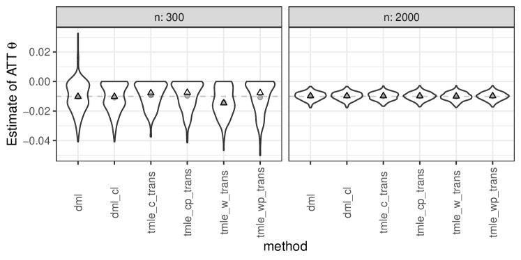
Figure S1: Six estimators’ sampling distributions, where trans stands for the variant of TMLE in Balzer et al. (2016). The bounds on $Q$ is set to be $[0,0.05]$. The horizontal dashed line is the truth. The gray dots and black triangles are the means and medians, respectively.

The sampling distributions of the TMLE variants proposed by Balzer et al. (2016) are presented in Fig. S1 and S2 in the Supplemental Material. All estimators perform similarly in relatively large samples ($n=2000$). When the sample size is small ($n=300$) and the known bounds on $Q$ are relatively tight ($[0,0.05]$), all versions of TMLE except tmle_w have substantially improved performance and appear similar to the clipped DML estimator. The variant of tmle_w performs worse as shown by a substantially increased bias and longer tail. When the known bounds are much wider ($[0,0.2]$), these TMLE variants perform slightly worse as shown by longer tails in the sampling distributions, indicating some sensitivity of such TMLE variants to the specified bounds. These results suggest that, when the outcome is rare and the sample size is relatively small, the variant developed by Balzer et al. (2016) might improve the performance of poorly-performing TMLE but harm well-performing TMLE. It is still an open question whether a particular version of TMLE is superior to the other versions in general.

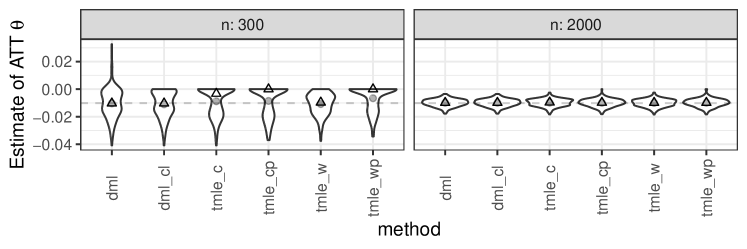
Figure 1: The six estimators’ sampling distributions. The horizontal dashed line is the truth. The gray dots and black triangles are the means and medians, respectively.

	$n=300$			$n=2000$
Method	Bias ($\times 10^{-4}$)	MSE ($\times 10^{-4}$)	CI coverage	Bias ($\times 10^{-4}$)	MSE ($\times 10^{-4}$)	CI coverage
dml	9.78	1.18	83%	-0.67	0.08	91%
dml_cl	2.80	0.96	83%	-0.67	0.08	91%
tmle_c	22.78	0.91	67.5%	0.38	0.07	91.5%
tmle_cp	15.03	1.02	65.5%	-0.93	0.09	91.5%
tmle_w	-1.02	0.53	81.5%	0.04	0.07	91.5%
tmle_wp	29.9	0.86	65.5%	-1.06	0.09	91.5%

Table 1: Monte Carlo estimates of the bias ${\mathbb{E}}[\hat{\theta}-\theta]$, Mean Squared Error (MSE) ${\mathbb{E}}[(\hat{\theta}-\theta)^{2}]$, and 95% Wald-CI coverage $\Pr(\theta\in\mathrm{CI})$ of the six estimators.

5 Proposed diagnosis for TMLE

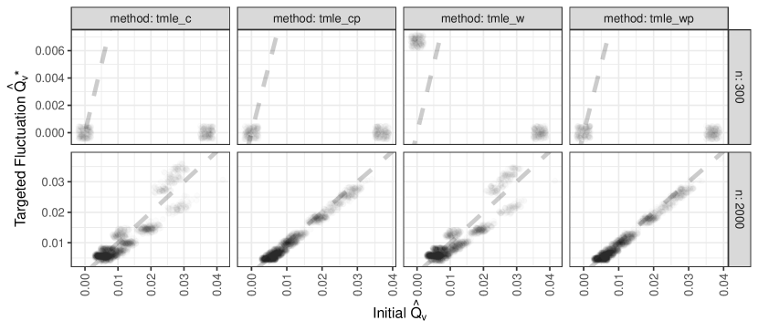
Figure S3: The fluctuated and the initial outcome regression estimators evaluated at each observed $X_{i}$ in two simulation runs. The points are jittered and semi-transparent for better visibility. The gray dashed line is the diagonal line $y=x$. Note the different y-axis scales between the two rows. The points appear far from the diagonal line in small samples ($n=300$, Row 1), indicating discordance between targeted fluctuation $\hat{Q}^{*}_{v}$ and initial $\hat{Q}_{v}$. In contrast, the points are closer to the diagonal line in relatively large samples ($n=2000$, Row 2), indicating more concordance.

To further investigate potential causes of the poorer small-sample performance of TMLE than DML estimators, I present the sampling distribution of the fluctuation coefficient $\epsilon^{*}_{v}$ of TMLE in Fig. 2. Sample mean relative absolute differences (MRAD), $n^{-1}\sum_{v=1}^{V}\sum_{i\in I_{v}}\left|\hat{Q}_{v}^{*}(X_{i})-\hat{Q}_{v}(X_{i})/\hat{Q}_{v}^{*}(X_{i})\right|$, between the fluctuation $\hat{Q}^{*}_{v}$ and the initial $\hat{Q}_{v}$ are presented in Fig. 3 in the supplemental material. I choose the fluctuation $\hat{Q}_{v}^{*}$ rather than the initial $\hat{Q}_{v}$ as the denominator because $\hat{Q}_{v}(X_{i})$ might equal zero exactly. In Fig. S3 in the supplemental material, I also plot the predicted values of the fluctuated outcome regression $\hat{Q}^{*}_{v}$ in the simulated data set against those of the initial outcome regression $\hat{Q}_{v}$ (i) in a simulation run where the sample size is small ($n=300$), the poor-performing TMLEs are almost zero, and DML estimators is closer to the truth, and (ii) in a simulation run with a relatively large sample size ($n=2000$).

One sufficient condition to justify TMLE is that the initial outcome regression estimator $\hat{Q}_{v}$ is close to the truth $Q$ and the magnitude of fluctuation is small. It is plausible that the fluctuation has a small magnitude in large samples because the targeting step refits the outcome regression based on a well-trained initial fit. Indeed, this appears to hold approximately in relatively large samples ($n=2000$), with $\epsilon^{*}_{v}$ and sample mean MRAD concentrating around zero (Fig. 2b, Fig. 3b), and $\hat{Q}^{*}_{v}(X_{i})$ similar to $\hat{Q}_{v}(X_{i})$ (Fig. S3 Row 2). However, in small samples ($n=300$), there is a high probability that the fluctuation has a large magnitude, namely $\epsilon^{*}_{v}$ and sample MRAD has huge magnitudes (Fig. 2a, Fig. 3a) and $\hat{Q}^{*}_{v}(X_{i})$ is far from $\hat{Q}_{v}(X_{i})$ (Fig. S3 Row 1). In this simulation, because of clipping $\operatorname{logit}\hat{Q}_{v}(x)$ into a large finite interval to account for $\hat{Q}_{v}(x)=0$, one scenario of a significant fluctuation is no cases in the data, although other scenarios also exist. In the simulation run shown in Fig. S3 Row 1, at least one fluctuation has a large magnitude (of order $10^{3}$ or even $10^{15}$) for all four versions of TMLEs.

Based on these simulation results, I conjecture that TMLE might perform unsatisfactorily in a given data if the magnitude $|\epsilon^{*}_{v}|$ of the fluctuation is large and if the predicted values of the fluctuated and initial outcome regressions are qualitatively different.

Therefore, it might be beneficial to check at least one of the following:

• For each fold $v$, after computing the fluctuated outcome regression estimator $\hat{Q}^{*}_{v}$, typically by fitting a generalized linear model with fitted coefficient $\epsilon^{*}_{v}$, if $|\epsilon^{*}_{v}|$ is extremely large (e.g., greater than 10), the TMLE might perform unsatisfactorily. When a pooled logistic regression is used for targeting, if the one fluctuation coefficient $\epsilon^{*}$ has an extremely large absolute value, the TMLE might perform unsatisfactorily.

• For every observation index $i$, compute the predicted value $\hat{Q}_{i}^{*}:=\hat{Q}_{v}^{*}(X_{i})$ and $\hat{Q}_{i}:=\hat{Q}_{v}(X_{i})$ for the fluctuated and initial outcome regression estimators, where $v$ is the fold containing observation $i$ (i.e., $i\in I_{v}$). Compute the sample MRAD, $n^{-1}\sum_{i=1}^{n}\left|\hat{Q}_{i}^{*}-\hat{Q}_{i}/\hat{Q}_{i}^{*}\right|$. If MRAD is extremely large (e.g., greater than 10), the TMLE might perform unsatisfactorily.

• Plot $\hat{Q}_{i}^{*}$ against $\hat{Q}_{i}$ for all observations in the data, for example, as Fig. S3 in the supplemental material. If many points appear far from the diagonal line, this indicates discordance between $\hat{Q}^{*}_{v}$ and $\hat{Q}_{v}$ and the TMLE might perform unsatisfactorily. Compared to $|\epsilon^{*}_{v}|$ and MRAD, this plot provides a more intuitive visualization of the concordance between $\hat{Q}^{*}_{v}$ and $\hat{Q}_{v}$.

The above thresholds for large $|\epsilon^{*}_{v}|$ and MRAD are chosen based on this simulation and are somewhat arbitrary.

All these diagnoses can be easily implemented because they use intermediate computation results from TMLE. It remains challenging to identify a clear theoretically justified threshold to determine whether the fluctuation is too large or acceptable. After removing TMLE estimates satisfying one of these conditions, the TMLE sampling distributions appear better (see Fig. 4). However, since excluding estimators based on diagnosis tools is conditioning on a subset of all realizations of the data, statistical properties of the procedure such as bias and CI coverage are not guaranteed by theory. As shown in Table 2, after excluding simulation runs based on the above diagnosis, for all estimators, the bias has become larger. The Wald-CI overcovers or undercover, but the coverage has improved when it undercovers. The MSE appears to remain similar. How to incorporate diagnosis into statistical procedures with theoretical guarantees is an interesting open question.

I conclude by remarking that TMLE might still perform well even if the fluctuation is large, for example, tmle_w in this simulation. Thus, a large fluctuation should be interpreted as a warning rather than a falsification of TMLE.

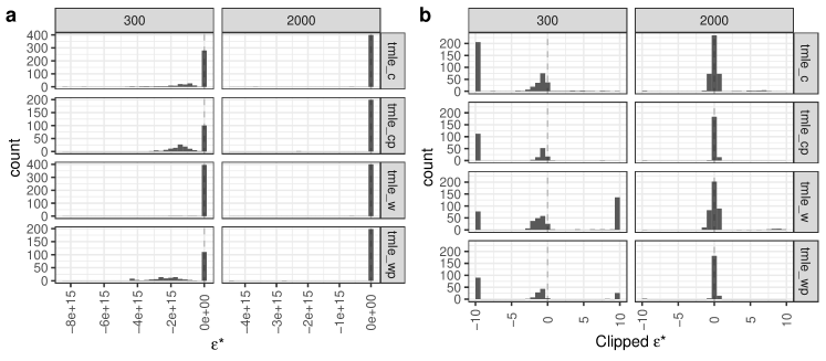
Figure 2: Histograms of the fluctuation coefficient $\epsilon^{*}_{v}$ or $\epsilon^{*}$ for the four versions of TMLE. Each column is a sample size and each row is a version of TMLE. The vertical dashed line represents no fluctuation, namely zero fluctuation coefficient. Subfigure (b) presents $\epsilon^{*}_{v}$ or $\epsilon^{*}$ clipped to fall in the interval $[-10,10]$; the clipping affects only six values on samples with $n=2000$.

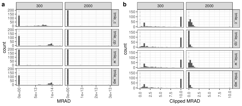
Figure 3: Sampling distributions of sample MRAD. Subfigure (b) presents MRAD clipped to fall in the interval $[0,10]$; the clipping affects only six values in all simulation runs with $n=2000$.

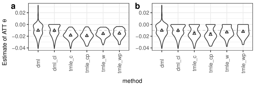
Figure 4: Plots similar to Fig. 1 after removing potentially problematic TMLE in small samples ($n=300$). In Subfigures (a) and (b), TMLE estimates with $|\epsilon^{*}_{v}|>10$ and sample MRAD greater than 10 are removed, respectively.

	Remove $|\epsilon^{*}_{v}|>10$			Remove $|\text{MRAD}|>10$
Method	Bias ($\times 10^{-4}$)	MSE ($\times 10^{-4}$)	CI coverage	Bias ($\times 10^{-4}$)	MSE ($\times 10^{-4}$)	CI coverage
dml	-46.22	1.05	100%	-17.28	0.98	81.1%
dml_cl	-48.64	0.97	100%	-18.81	0.93	81.1%
tmle_c	-78.79	1.19	98.9%	-37.58	1.14	79.5%
tmle_cp	-81.81	1.45	96.8%	-37.60	1.35	76.2%
tmle_w	-59.23	0.85	100%	-26.53	0.85	81.1%
tmle_wp	-37.30	0.84	96.8%	-6.45	0.86	76.2%

Table 2: Table similar to Table. 1 after removing potentially problematic TMLE in small samples ($n=300$).

6 Discussion

I show in a simulation that in finite samples, a plug-in estimator might perform worse than a non-plug-in estimator sharing the same large-sample properties, even though the plug-in estimator always respects known bounds on the parameter while the non-plug-in estimator might not.

This example is cherry-picked and has several limitations. In practice, when the outcome is rare, other sampling schemes such as case-control are often adopted to overcome the challenge of too few cases. However, a preliminary analysis with data from a small cohort or cross-sectional study might fit this example. If the propensity score is estimated with a flexible machine learning algorithm that might overfit in small samples (e.g., without clipping), the propensity score estimator is more vulnerable to overfitting and near positivity violation, and thus DML estimators may perform much worse than TMLE in small samples. If the estimand is the ATT instead of the mean counterfactual outcome among treated, TMLE might also perform well due to the small magnitude of its bias. Nevertheless, the mean counterfactual outcome may still be of scientific interest because it informs the counterfactual result of one intervention. It is also closely related to covariate shift problems in machine learning (Lei and Candès, 2021; Qiu et al., 2023).

I use TMLE and DML estimators as examples from the two categories of estimators—plug-in and non-plug-in—but counterexamples might exist for other pairs of estimators with the same large-sample behaviors. I further propose methods to diagnose whether TMLE might perform worse than DML estimators due to a large fluctuation based on this simulation. Because intuitive arguments such as the plug-in principle may be flawed, more rigorous theoretical justification is needed to understand and compare the finite-sample performance of highly flexible estimators in general.

Supplement to “Non-Plug-In Estimators Could Outperform Plug-In Estimators:
a Cautionary Note and a Diagnosis”

I present the six estimators of the mean counterfactual outcome corresponding to control among the treated, ${\mathbb{E}}[Y(0)\mid A=1]$, described in Section 3. The major differences (i) among the four TMLEs, and (ii) between the two DML estimators, are highlighted in blue. Methods to estimate the nuisance functions are described in Section 3. The method to compute standard errors and construct Wald-CI is non-unique; only one simple working method is described. I use $z_{\alpha}$ to denote the $(1-\alpha/2)$-quantile of the standard normal distribution. After obtaining an estimator $\hat{\psi}$ of $\psi$, the ATT $\theta$ is estimated by

$$\hat{\theta}:=\frac{\sum_{i=1}^{n}{\mathbbm{1}}(A_{i}=1)Y_{i}}{\sum_{i=1}^{n}{\mathbbm{1}}(A_{i}=1)}-\hat{\psi}.$$

Algorithm S1 Estimator tmle_c of $\psi={\mathbb{E}}[Y(0)\mid A=1]$.

1:Randomly split data into $V$ folds of approximately equal sizes. Denote the index sets of observations in and out of fold $v$ by $I_{v}$ and $I_{v}^{C}$, respectively.

2:for $v=1,\ldots,V$ do

3:     Estimate the outcome regression $Q$ by $\hat{Q}_{v}$ trained using data in the control group ($A_{i}=0$) in $I_{v}^{C}$ (namely outside fold $v$).

4:     Estimate the propensity score $g$ by $\hat{g}_{v}$ trained using data in $I_{v}^{C}$ (namely outside fold $v$).

5:     Estimate the marginal probability of treatment $\pi$ by $\hat{\pi}_{v}:=\sum_{i\in I_{v}}{\mathbbm{1}}(A_{i}=1)/|I_{v}|$.

6:     Define $H_{v}(x):=\frac{\hat{g}_{v}(X)}{\hat{\pi}_{v}\{1-\hat{g}_{v}(X)\}}$. $\triangleright$ (Define clever covariate)

7:     Using observations in $I_{v}$ in the control group ($A_{i}=0$), run a logistic regression with outcome $Y_{i}$, offset $\operatorname{logit}\hat{Q}_{v}(X_{i})$, covariate $H_{v}(X_{i})$, and no intercept. Denote the fitted slope by $\epsilon^{*}_{v}$. $\triangleright$ (Targeting within each fold)

8:     Define the targeted outcome regression $\hat{Q}^{*}_{v}(x):=\operatorname{expit}\left\{\operatorname{logit}\hat{Q}_{v}(x)+\epsilon^{*}_{v}H_{v}(x)\right\}$.

9:     Compute the plug-in estimator based on the targeted outcome regression, namely

$$\hat{\psi}_{v}:=\frac{\sum_{i\in I_{v}}{\mathbbm{1}}(A_{i}=1)\hat{Q}^{*}_{v}(X_{i})}{\sum_{i\in I_{v}}{\mathbbm{1}}(A_{i}=1)}.$$

10:Output the cross-fit estimator $\hat{\psi}=n^{-1}\sum_{v=1}^{V}|I_{v}|\hat{\psi}_{v}$.

11:Wald-CI: Compute the standard error $\mathrm{SE}:=\{n^{-1}\sum_{v=1}^{V}\sum_{i\in I_{v}}D(\hat{Q}_{v}^{*},\hat{g}_{v},\hat{\pi}_{v},\hat{\psi})(X_{i},A_{i},Y_{i})^{2}\}^{-1/2}/\sqrt{n}$ and construct two-sided $(1-\alpha)$-level Wald-CI $\hat{\psi}\pm z_{\alpha}\times\mathrm{SE}$.

Algorithm S2 Estimator tmle_w of $\psi={\mathbb{E}}[Y(0)\mid A=1]$.

1:Randomly split data into $V$ folds of approximately equal sizes. Denote the index sets of observations in and out of fold $v$ by $I_{v}$ and $I_{v}^{C}$, respectively.

2:for $v=1,\ldots,V$ do

3:     Estimate the outcome regression $Q$ by $\hat{Q}_{v}$ trained using data in the control group ($A_{i}=0$) in $I_{v}^{C}$ (namely outside fold $v$).

4:     Estimate the propensity score $g$ by $\hat{g}_{v}$ trained using data in $I_{v}^{C}$ (namely outside fold $v$).

5:     Estimate the marginal probability of treatment $\pi$ by $\hat{\pi}_{v}:=\sum_{i\in I_{v}}{\mathbbm{1}}(A_{i}=1)/|I_{v}|$.

6:     Define $W_{v}(a,x):=\frac{{\mathbbm{1}}(a=0)\hat{g}_{v}(x)}{\hat{\pi}_{v}\{1-\hat{g}_{v}(x)\}}$. $\triangleright$ (Define weight)

7:     Using data in $I_{v}$, run an intercept-only logistic regression with outcome $Y_{i}$, offset $\operatorname{logit}\hat{Q}_{v}(X_{i})$, and weight $W_{v}(A_{i},X_{i})$. Denote the fitted intercept by $\epsilon^{*}_{v}$. $\triangleright$ (Targeting within each fold)

8:     Define the targeted outcome regression $\hat{Q}^{*}_{v}(x):=\operatorname{expit}\left\{\operatorname{logit}\hat{Q}_{v}(x)+\epsilon^{*}_{v}\right\}$.

9:     Compute the plug-in estimator based on the targeted outcome regression, namely

$$\hat{\psi}_{v}:=\frac{\sum_{i\in I_{v}}{\mathbbm{1}}(A_{i}=1)\hat{Q}^{*}_{v}(X_{i})}{\sum_{i\in I_{v}}{\mathbbm{1}}(A_{i}=1)}.$$

10:Output the cross-fit estimator $\hat{\psi}=n^{-1}\sum_{v=1}^{V}|I_{v}|\hat{\psi}_{v}$.

11:Wald-CI: Compute the standard error $\mathrm{SE}:=\{n^{-1}\sum_{v=1}^{V}\sum_{i\in I_{v}}D(\hat{Q}_{v}^{*},\hat{g}_{v},\hat{\pi}_{v},\hat{\psi})(X_{i},A_{i},Y_{i})^{2}\}^{-1/2}/\sqrt{n}$ and construct two-sided $(1-\alpha)$-level Wald-CI $\hat{\psi}\pm z_{\alpha}\times\mathrm{SE}$.

Algorithm S3 Estimator tmle_cp of $\psi={\mathbb{E}}[Y(0)\mid A=1]$.

1:Randomly split data into $V$ folds of approximately equal sizes. Denote the index sets of observations in and out of fold $v$ by $I_{v}$ and $I_{v}^{C}$, respectively.

2:for $v=1,\ldots,V$ do

3:     Estimate the outcome regression $Q$ by $\hat{Q}_{v}$ trained using data in the control group ($A_{i}=0$) in $I_{v}^{C}$ (namely outside fold $v$).

4:     Estimate the propensity score $g$ by $\hat{g}_{v}$ trained using data in $I_{v}^{C}$ (namely outside fold $v$).

5:     Estimate the marginal probability of treatment $\pi$ by $\hat{\pi}_{v}:=\sum_{i\in I_{v}}{\mathbbm{1}}(A_{i}=1)/|I_{v}|$.

6:     For each $i\in I_{v}$, define $\hat{Q}_{i}:=\hat{Q}_{v}(X_{i})$ and $H_{i}:=\frac{\hat{g}_{v}(X_{i})}{\hat{\pi}_{v}\{1-\hat{g}_{v}(X_{i})\}}$. $\triangleright$ (Define clever covariate)

7:Using observations in the control group ($A=0$) in the entire dataset, run a logistic regression with outcome $Y_{i}$, offset $\operatorname{logit}\hat{Q}_{v}(X)$, covariate $H_{v}(X)$, and no intercept. Denote the fitted slope by $\epsilon^{*}$. $\triangleright$ (Targeting over the entire, namely pooled, data)

8:Compute the targeted outcome regression evaluated at each observation $\hat{Q}^{*}_{i}:=\operatorname{expit}\left\{\operatorname{logit}\hat{Q}_{i}+\epsilon^{*}H_{i}\right\}$.

9:Output the plug-in estimator based on the targeted outcome regression

$$\hat{\psi}:=\frac{\sum_{i=1}^{n}{\mathbbm{1}}(A_{i}=1)\hat{Q}^{*}_{i}}{\sum_{i=1}^{n}{\mathbbm{1}}(A_{i}=1)}.$$

10:Wald-CI: With $\hat{Q}_{v}^{*}:=\operatorname{expit}\left\{\operatorname{logit}\hat{Q}+\epsilon^{*}\frac{\hat{g}_{v}}{\hat{\pi}_{v}\{1-\hat{g}_{v}\}}\right\}$, compute the standard error $\mathrm{SE}:=\{n^{-1}\sum_{v=1}^{V}\sum_{i\in I_{v}}D(\hat{Q}_{v}^{*},\hat{g}_{v},\hat{\pi}_{v},\hat{\psi})(X_{i},A_{i},Y_{i})^{2}\}^{-1/2}/\sqrt{n}$ and construct two-sided $(1-\alpha)$-level Wald-CI $\hat{\psi}\pm z_{\alpha}\times\mathrm{SE}$.

Algorithm S4 Estimator tmle_wp of $\psi={\mathbb{E}}[Y(0)\mid A=1]$.

1:Randomly split data into $V$ folds of approximately equal sizes. Denote the index sets of observations in and out of fold $v$ by $I_{v}$ and $I_{v}^{C}$, respectively.

2:for $v=1,\ldots,V$ do

3:     Estimate the outcome regression $Q$ by $\hat{Q}_{v}$ trained using data in the control group ($A_{i}=0$) in $I_{v}^{C}$ (namely outside fold $v$).

4:     Estimate the propensity score $g$ by $\hat{g}_{v}$ trained using data in $I_{v}^{C}$ (namely outside fold $v$).

5:     Estimate the marginal probability of treatment $\pi$ by $\hat{\pi}_{v}:=\sum_{i\in I_{v}}{\mathbbm{1}}(A_{i}=1)/|I_{v}|$.

6:     For each $i\in I_{v}$, define $\hat{Q}_{i}:=\hat{Q}_{v}(X_{i})$ and $W_{i}:=\frac{{\mathbbm{1}}(A_{i}=0)\hat{g}_{v}(X_{i})}{\hat{\pi}_{v}\{1-\hat{g}_{v}(X_{i})\}}$. $\triangleright$ (Define weight)

7:Using observations in the entire dataset, run an intercept-only logistic regression with outcome $Y_{i}$, offset $\operatorname{logit}\hat{Q}_{i}$, and weight $W_{i}$. Denote the fitted intercept by $\epsilon^{*}$. $\triangleright$ (Targeting over the entire, namely pooled, data)

8:Compute the targeted outcome regression evaluated at each observation $\hat{Q}^{*}_{i}:=\operatorname{expit}\left\{\operatorname{logit}\hat{Q}_{i}+\epsilon^{*}\right\}$.

9:Compute the plug-in estimator based on the targeted outcome regression

$$\hat{\psi}:=\frac{\sum_{i=1}^{n}{\mathbbm{1}}(A_{i}=1)\hat{Q}^{*}_{i}}{\sum_{i=1}^{n}{\mathbbm{1}}(A_{i}=1)}.$$

10:Wald-CI: With $\hat{Q}_{v}^{*}:=\operatorname{expit}\left\{\operatorname{logit}\hat{Q}+\epsilon^{*}\right\}$, compute the standard error $\mathrm{SE}:=\{n^{-1}\sum_{v=1}^{V}\sum_{i\in I_{v}}D(\hat{Q}_{v}^{*},\hat{g}_{v},\hat{\pi}_{v},\hat{\psi})(X_{i},A_{i},Y_{i})^{2}\}^{-1/2}/\sqrt{n}$ and construct two-sided $(1-\alpha)$-level Wald-CI $\hat{\psi}\pm z_{\alpha}\times\mathrm{SE}$.

Algorithm S5 Estimator dml of $\psi={\mathbb{E}}[Y(0)\mid A=1]$.

1:Randomly split data into $V$ folds of approximately equal sizes. Denote the index sets of observations in and out of fold $v$ by $I_{v}$ and $I_{v}^{C}$, respectively.

2:for $v=1,\ldots,V$ do

3:     Estimate the outcome regression $Q$ by $\hat{Q}_{v}$ trained using data in the control group ($A_{i}=0$) in $I_{v}^{C}$ (namely outside fold $v$).

4:     Estimate the propensity score $g$ by $\hat{g}_{v}$ trained using data in $I_{v}^{C}$ (namely outside fold $v$).

5:     Estimate the marginal probability of treatment $\pi$ by $\hat{\pi}_{v}:=\sum_{i\in I_{v}}{\mathbbm{1}}(A_{i}=1)/|I_{v}|$.

6:     Compute the DML estimator

$$\hat{\psi}_{v}:=\frac{1}{|I_{v}|}\sum_{i\in I_{v}}\left\{\frac{{\mathbbm{1}}(A_{i}=1)\hat{Q}_{v}(X_{i})}{{\mathbbm{1}}(A_{i}=1)}+\frac{{\mathbbm{1}}(A_{i}=0)\hat{g}_{v}(X_{i})}{\hat{\pi}_{v}\{1-\hat{g}_{v}(X_{i})\}}\{Y_{i}-\hat{Q}_{v}(X_{i})\}\right\}.$$

7:Output the cross-fit DML estimator $\hat{\psi}=n^{-1}\sum_{v=1}^{V}|I_{v}|\hat{\psi}_{v}$.

8:Wald-CI: Compute the standard error $\mathrm{SE}:=\{n^{-1}\sum_{v=1}^{V}\sum_{i\in I_{v}}D(\hat{Q}_{v},\hat{g}_{v},\hat{\pi}_{v},\hat{\psi})(X_{i},A_{i},Y_{i})^{2}\}^{-1/2}/\sqrt{n}$ and construct two-sided $(1-\alpha)$-level Wald-CI $\hat{\psi}\pm z_{\alpha}\times\mathrm{SE}$.

Algorithm S6 Estimator dml_cl of $\psi={\mathbb{E}}[Y(0)\mid A=1]$.

1:Randomly split data into $V$ folds of approximately equal sizes. Denote the index sets of observations in and out of fold $v$ by $I_{v}$ and $I_{v}^{C}$, respectively.

2:for $v=1,\ldots,V$ do

3:     Estimate the outcome regression $Q$ by $\hat{Q}_{v}$ trained using data in the control group ($A_{i}=0$) in $I_{v}^{C}$ (namely outside fold $v$).

4:     Estimate the propensity score $g$ by $\hat{g}_{v}$ trained using data in $I_{v}^{C}$ (namely outside fold $v$).

5:     Estimate the marginal probability of treatment $\pi$ by $\hat{\pi}_{v}:=\sum_{i\in I_{v}}{\mathbbm{1}}(A_{i}=1)/|I_{v}|$.

6:     Compute the DML estimator

$$\hat{\psi}_{v}:=\frac{1}{|I_{v}|}\sum_{i\in I_{v}}\left\{\frac{{\mathbbm{1}}(A_{i}=1)\hat{Q}_{v}(X_{i})}{{\mathbbm{1}}(A_{i}=1)}+\frac{{\mathbbm{1}}(A_{i}=0)\hat{g}_{v}(X_{i})}{\hat{\pi}_{v}\{1-\hat{g}_{v}(X_{i})\}}\{Y_{i}-\hat{Q}_{v}(X_{i})\}\right\}.$$

7:Compute the cross-fit DML estimator $\hat{\psi}=n^{-1}\sum_{v=1}^{V}|I_{v}|\hat{\psi}_{v}$.

8:Output $\hat{\psi}^{\dagger}:=\min\{\max\{\hat{\psi},0\},1\}$. $\triangleright$ (Clipping to $[0,1]$)

9:Wald-CI: Compute the standard error $\mathrm{SE}:=\{n^{-1}\sum_{v=1}^{V}\sum_{i\in I_{v}}D(\hat{Q}_{v},\hat{g}_{v},\hat{\pi}_{v},\hat{\psi}^{\dagger})(X_{i},A_{i},Y_{i})^{2}\}^{-1/2}/\sqrt{n}$ and construct two-sided $(1-\alpha)$-level Wald-CI $\hat{\psi}^{\dagger}\pm z_{\alpha}\times\mathrm{SE}$.

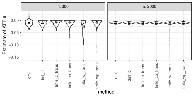
Figure S2: Figure similar to Fig. S1 with the bounds on $Q$ set to be $[0,0.2]$.

References

- Balakrishnan et al. (2023) S. Balakrishnan, E. H. Kennedy, and L. Wasserman. The Fundamental Limits of Structure-Agnostic Functional Estimation. arXiv preprint arXiv:2305.04116v1, 2023.
- Balzer et al. (2016) L. Balzer, J. Ahern, S. Galea, and M. Van der Laan. Estimating Effects with Rare Outcomes and High Dimensional Covariates: Knowledge is Power. Epidemiologic Methods, 5(1):1–18, 2016. ISSN 2161962X. doi: 10.1515/em-2014-0020.
- Barash et al. (2012) J. A. Barash, R. A. Desai, and H. S. Patwa. Veterans health administration information systems as a resource for rare disorders research: Creutzfeldt-Jakob disease as a paradigm. Military Medicine, 177(11):1343–1347, 2012. ISSN 00264075. doi: 10.7205/MILMED-D-12-00198. URL https://dx.doi.org/10.7205/MILMED-D-12-00198.
- Bickel et al. (1993) P. J. Bickel, C. A. Klaassen, Y. Ritov, and J. A. Wellner. Efficient and Adaptive Estimation for Semiparametric Models., volume 4. Johns Hopkins University Press, 1993. ISBN 978-0-387-98473-5. doi: 10.2307/2533465.
- Brown et al. (2001) L. D. Brown, T. T. Cai, and A. Das Gupta. Interval estimation for a binomial proportion. Statistical Science, 16(2):101–117, 2001. ISSN 08834237. doi: 10.1214/ss/1009213286.
- Chen and Guestrin (2016) T. Chen and C. Guestrin. XGBoost: A scalable tree boosting system. Proceedings of the ACM SIGKDD International Conference on Knowledge Discovery and Data Mining, 13-17-Augu:785–794, 2016. doi: 10.1145/2939672.2939785.
- Chernozhukov et al. (2017) V. Chernozhukov, D. Chetverikov, M. Demirer, E. Duflo, C. Hansen, and W. Newey. Double/debiased/Neyman machine learning of treatment effects. American Economic Review, 107(5):261–265, 2017. ISSN 00028282. doi: 10.1257/aer.p20171038.
- Chernozhukov et al. (2018) V. Chernozhukov, D. Chetverikov, M. Demirer, E. Duflo, C. Hansen, W. Newey, and J. Robins. Double/debiased machine learning for treatment and structural parameters. Econometrics Journal, 21(1):C1–C68, 2018. ISSN 1368423X. doi: 10.1111/ectj.12097.
- Gruber and Van Der Laan (2010) S. Gruber and M. J. Van Der Laan. A targeted maximum likelihood estimator of a causal effect on a bounded continuous outcome. International Journal of Biostatistics, 6(1), 2010. ISSN 15574679. doi: 10.2202/1557-4679.1260.
- Gruber and Van Der Laan (2014) S. Gruber and M. J. Van Der Laan. Targeted minimum loss based estimation of a causal effect on an outcome with known conditional bounds. International Journal of Biostatistics, 8(1), 2014. ISSN 15574679. doi: 10.1515/1557-4679.1413.
- Guo et al. (2023) A. Guo, D. Benkeser, and R. Nabi. Targeted Machine Learning for Average Causal Effect Estimation Using the Front-Door Functional. arXiv preprint arXiv:2312.10234v1, 2023. URL http://arxiv.org/abs/2312.10234.
- Hahn (1998) J. Hahn. On the Role of the Propensity Score in Efficient Semiparametric Estimation of Average Treatment Effects. Econometrica, 66(2):315, 1998. ISSN 00129682. doi: 10.2307/2998560.
- Jin and Syrgkanis (2024) J. Jin and V. Syrgkanis. Structure-agnostic Optimality of Doubly Robust Learning for Treatment Effect Estimation. arXiv preprint arXiv:2402.14264, 2024.
- Kennedy (2022) E. H. Kennedy. Semiparametric doubly robust targeted double machine learning: a review. arXiv preprint arXiv:2203.06469v2, 2022.
- Lei and Candès (2021) L. Lei and E. J. Candès. Conformal inference of counterfactuals and individual treatment effects. Journal of the Royal Statistical Society. Series B: Statistical Methodology, 83(5):911–938, 2021. ISSN 14679868. doi: 10.1111/rssb.12445.
- Levy (2018) J. Levy. An Easy Implementation of CV-TMLE. arXiv preprint arXiv:1811.04573v2, 2018. URL http://arxiv.org/abs/1811.04573.
- Levy et al. (2018) J. Levy, M. van der Laan, A. Hubbard, and R. Pirracchio. A Fundamental Measure of Treatment Effect Heterogeneity. arXiv preprint arXiv:1811.03745v3, 2018.
- Li et al. (2022) H. Li, S. Rosete, J. Coyle, R. V. Phillips, N. S. Hejazi, I. Malenica, B. F. Arnold, J. Benjamin-Chung, A. Mertens, J. M. Colford, M. J. van der Laan, and A. E. Hubbard. Evaluating the robustness of targeted maximum likelihood estimators via realistic simulations in nutrition intervention trials. Statistics in Medicine, 41(12):2132–2165, 2022. ISSN 10970258. doi: 10.1002/sim.9348.
- McCann et al. (2006) L. J. McCann, A. D. Juggins, S. M. Maillard, L. R. Wedderburn, J. E. Davidson, K. J. Murray, and C. A. Pilkington. The Juvenile Dermatomyositis National Registry and Repository (UK and Ireland) - Clinical characteristics of children recruited within the first 5 yr. Rheumatology, 45(10):1255–1260, 2006. ISSN 14620324. doi: 10.1093/rheumatology/kel099. URL https://dx.doi.org/10.1093/rheumatology/kel099.
- Neyman (1923) J. Neyman. Sur les applications de la théorie des probabilités aux expériences agricoles: Essay des principles. (Excerpts reprinted and translated to English, 1990). Statistical Science, 5:463–472, 1923.
- Ogburn and Shpitser (2021) E. L. Ogburn and I. Shpitser. Causal Modelling: The Two Cultures. Observational Studies, 7(1):179–183, 2021. ISSN 27673324. doi: 10.1353/obs.2021.0006.
- Pfanzagl (1985) J. Pfanzagl. Contributions to a general asymptotic statistical theory, volume 3 of Lecture Notes in Statistics. Springer New York, New York, NY, 1985. ISBN 978-0-387-90776-5. doi: 10.1524/strm.1985.3.34.379.
- Pfanzagl (1990) J. Pfanzagl. Estimation in semiparametric models. pages 17–22. Springer, New York, NY, 1990. doi: 10.1007/978-1-4612-3396-1˙5.
- Qiu et al. (2023) H. Qiu, E. Dobriban, and E. T. Tchetgen. Prediction sets adaptive to unknown covariate shift. Journal of the Royal Statistical Society. Series B: Statistical Methodology, 85(5):1680–1705, 2023. ISSN 14679868. doi: 10.1093/jrsssb/qkad069.
- Robins et al. (1994) J. M. Robins, A. Rotnitzky, and L. P. Zhao. Estimation of regression coefficients when some regressors are not always observed. Journal of the American Statistical Association, 89(427):846–866, 1994. ISSN 1537274X. doi: 10.1080/01621459.1994.10476818.
- Robins et al. (1995) J. M. Robins, A. Rotnitzky, and L. P. Zhao. Analysis of semiparametric regression models for repeated outcomes in the presence of missing data. Journal of the American Statistical Association, 90(429):106–121, 1995. ISSN 1537274X. doi: 10.1080/01621459.1995.10476493.
- Rubin (1974) D. B. Rubin. Estimating causal effects of treatments in randomized and nonrandomized studies. Technical Report 5, 1974.
- Rytgaard et al. (2021) H. C. W. Rytgaard, F. Eriksson, and M. Van der Laan. Estimation of time-specific intervention effects on continuously distributed time-to-event outcomes by targeted maximum likelihood estimation. arXiv preprint arXiv:2106.11009v1, 2021.
- Schick (1986) A. Schick. On Asymptotically Efficient Estimation in Semiparametric Models. The Annals of Statistics, 14(3):1139–1151, 1986. ISSN 0090-5364. doi: 10.1214/aos/1176350055.
- Smith et al. (2023) M. J. Smith, R. V. Phillips, M. A. Luque-Fernandez, and C. Maringe. Application of targeted maximum likelihood estimation in public health and epidemiological studies: a systematic review. Annals of Epidemiology, 86:34–48.e28, 2023. ISSN 18732585. doi: 10.1016/j.annepidem.2023.06.004. URL https://doi.org/10.1016/j.annepidem.2023.06.004.
- Tran et al. (2019) L. Tran, C. Yiannoutsos, K. Wools-Kaloustian, A. Siika, M. Van Der Laan, and M. Petersen. Double Robust Efficient Estimators of Longitudinal Treatment Effects: Comparative Performance in Simulations and a Case Study. International Journal of Biostatistics, 15(2), 2019. ISSN 15574679. doi: 10.1515/ijb-2017-0054.
- Tran et al. (2023) L. Tran, M. Petersen, J. Schwab, and M. J. van der Laan. Robust variance estimation and inference for causal effect estimation. Journal of Causal Inference, 11(1), 2023. doi: 10.1515/jci-2021-0067.
- van der Laan (2019) M. J. van der Laan. TMLE versus the one-step estimator · The Research Group of Mark van der Laan, 2019. URL https://vanderlaan-lab.org/2019/05/10/tmle-versus-the-one-step-estimator/.
- Van der Laan and Rose (2018) M. J. Van der Laan and S. Rose. Targeted Learning in Data Science. Springer, 2018. ISBN 978-3-319-65303-7. doi: 10.1007/978-3-319-65304-4.
- van der Laan and Rubin (2006) M. J. van der Laan and D. Rubin. Targeted Maximum Likelihood Learning. The International Journal of Biostatistics, 2(1), jan 2006. ISSN 1557-4679. doi: 10.2202/1557-4679.1043.
- Van Der Laan et al. (2007) M. J. Van Der Laan, E. C. Polley, and A. E. Hubbard. Super learner. Statistical Applications in Genetics and Molecular Biology, 6(1), 2007. ISSN 15446115. doi: 10.2202/1544-6115.1309.
- van der Laan et al. (2013) M. J. van der Laan, M. Petersen, and W. Zheng. Estimating the Effect of a Community-Based Intervention with Two Communities. Journal of Causal Inference, 1(1):83–106, 2013. ISSN 2193-3677. doi: 10.1515/jci-2012-0011.
- van der Vaart and Wellner (1996) A. van der Vaart and J. Wellner. Weak Convergence and Empirical Processes: With Applications to Statistics. Springer Series in Statistics. Springer, 1996. ISBN 0387946403.
- Venables and Ripley (2002) W. N. Venables and B. D. Ripley. Modern Applied Statistics with S. Statistics and Computing. Springer New York, New York, NY, fourth edition, 2002. ISBN 978-1-4419-3008-8. doi: 10.1007/978-0-387-21706-2.
- Wakefield (2013) J. Wakefield. Bayesian and Frequentist Regression Methods. Springer Science & Business Media, 2013. ISBN 978-1-4419-0924-4. doi: 10.1007/978-1-4419-0925-1.
- Wang et al. (2017) A. Wang, R. A. Nianogo, and O. A. Arah. G-computation of average treatment effects on the treated and the untreated. BMC Medical Research Methodology, 17(1), 2017. ISSN 14712288. doi: 10.1186/s12874-016-0282-4.
- Wright and Ziegler (2017) M. N. Wright and A. Ziegler. Ranger: A fast implementation of random forests for high dimensional data in C++ and R. Journal of Statistical Software, 77(1):1–17, 2017. ISSN 15487660. doi: 10.18637/jss.v077.i01.
- Yang et al. (2022) Y. Yang, A. K. Kuchibhotla, and E. Tchetgen Tchetgen. Doubly Robust Calibration of Prediction Sets under Covariate Shift. arXiv preprint arXiv:2203.01761v1, 2022. doi: 10.48550/arxiv.2203.01761.
- Zheng and van der Laan (2011) W. Zheng and M. J. van der Laan. Cross-Validated Targeted Minimum-Loss-Based Estimation. In Targeted Learning, pages 459–474. Springer, New York, NY, 2011. doi: 10.1007/978-1-4419-9782-1˙27.