No Screening is More Efficient with Multiple Objects

Abstract

We study efficient mechanism design for allocating multiple heterogeneous objects. We aim to maximize the residual surplus, the total value generated from an allocation minus the costs for screening agents’ values. We discover a robust trend indicating that no-screening mechanisms such as serial dictatorship with exogenous priority order tend to perform better as the variety of goods increases. We analyze the underlying reasons by characterizing efficient mechanisms in a stylized environment. We also apply an automated mechanism design approach to numerically derive efficient mechanisms and validate the trend in general environments. Building on this implication, we propose the register-invite-book system (RIB) as an efficient system for scheduling vaccination against pandemic diseases.

Keywords: Money Burning, Multi-dimensional Types, Pandemic Vaccine, Extreme Value Theory, Automated Mechanism Design

1 Introduction

Policymakers often face the challenge of allocating scarce resources in the presence of information asymmetry. It is desirable to allocate goods to those who truly need them, i.e., agents with high valuations. However, when tractable screening devices such as monetary transfers are unavailable, screening can be costly. For instance, while a first-come, first-served (FCFS) mechanism incentivizes high-value agents to arrive early and secure the goods, it significantly wastes effort. By contrast, a lottery-based mechanism prevents wasted effort but risks high-value agents not receiving the goods. To maximize social welfare (i.e., residual surplus, the sum of agents’ payoffs from the allocation minus the sum of screening costs wasted), we must evaluate the tradeoff between allocative efficiency and screening costs.

Despite its practical importance, the literature has not fully characterized an efficient screening mechanism, except for the environment with single-dimensional types representing the values for homogeneous goods (Hartline and Roughgarden, 2008). Many real-world problems involve multiple heterogeneous objects. The scheduling of vaccine appointments during the COVID-19 pandemic was a prominent example—reservation slots, each of which specifies when, where, and which vaccines will be administered, are highly heterogeneous goods, and potential recipients have diverse preferences over slots. In such an environment, each agent’s effort level affects not only whether they can obtain a good (vaccine) but also which good (reservation slot) they can choose, influencing the performance of mechanisms. Given the possibility of another pandemic requiring the swift and efficient distribution of vaccines, a policy recommendation for this problem is highly demanded by society.

In this paper, we study efficient screening mechanisms for allocating heterogeneous objects. Agents have multi-dimensional types representing their values for each object, whereas they only have a unit demand. Agents can signal their values by making efforts as a form of payment. The central planner aims to choose the mechanism that maximizes residual surplus from a variety of options. A potential candidate is serial dictatorship with exogenous order (SD), under which agents sequentially select their most preferred goods from the remaining ones according to a predetermined order. SD is a no-screening mechanism in that agents cannot improve their allocations by paying the effort cost. Another candidate is the Vickrey-Clarke-Groves mechanism (VCG), which induces full screening of agents’ values to achieve allocative efficiency while incurring substantial screening costs. Besides these, the central planner has numerous options regarding the extent of screening costs to incur and how to allocate goods based on agents’ revealed values. Characterization of efficient mechanisms for such a multi-dimensional environment is widely believed challenging because we cannot pin down the payment rule from an allocation rule and strategy-proofness using the revenue equivalence theorem (Myerson, 1981).

This study discovers a robust trend indicating that as the variety of goods increases, no-screening mechanisms such as SD tend to perform better. First, to explore the reasons behind this, we analyze a stylized environment that allows for analytical characterization. Agents attempt to choose their preferred goods from a variety. Consequently, agents’ values in a multi-object problem can largely be represented by the largest order statistic of their values for individual goods. We examine the behavior of the largest order statistic as the sample size increases using extreme value theory, proving that the performance of no-screening mechanisms improves. Second, we employ the rapidly advancing technology of automated mechanism design (Sandholm, 2003; Conitzer and Sandholm, 2004; Dütting et al., 2019) to numerically explore efficient mechanisms in more general environments beyond the stylized setup. In many settings involving multiple goods, no-screening mechanisms perform well, indicating that the strong assumptions of the stylized environment (such as large market, symmetric capacity, and i.i.d. values) do not critically impact the implications. Finally, we consider a real-world application: scheduling vaccine appointments during the COVID-19 pandemic. We discuss that the register-invite-book system (RIB), a sequential-form implementation of SD, is an effective method for distributing a large number of heterogeneous goods, such as reservation slots for vaccines.

In a stylized environment developed for theoretical analyses, we consider a large market model with a continuum of agents and objects. Each agent consumes at most one object, and objects are categorized into a finite number of types with equal capacities. Each agent’s value for each object type is drawn i.i.d. from a marginal value distribution. In this environment, all types of goods are equally popular and scarce; thus, agents obtain either their favorite object or nothing, under any mechanisms of interest (satisfying symmetry and ex post efficiency, defined later). Accordingly, this problem can be reduced to a single-dimensional environment, where each agent’s value for the single-dimensional problem is the value for her favorite object, i.e., the largest order statistic, in the original multi-dimensional problem.

The value distribution of each agent’s favorite object is crucial for the nature of efficient mechanisms. For a single-dimensional environment, Hartline and Roughgarden (2008) prove that no screening is efficient when the value distribution has an increasing hazard rate (hereafter IHR), and full screening is efficient when it has a decreasing hazard rate (DHR). In other cases, an efficient mechanism is obtained through Myerson’s (1981) ironing. Accordingly, by evaluating the distribution of the largest order statistic, we can characterize an efficient mechanism in the stylized environment.

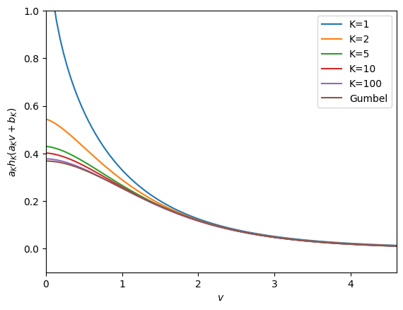
(a) Probability Density

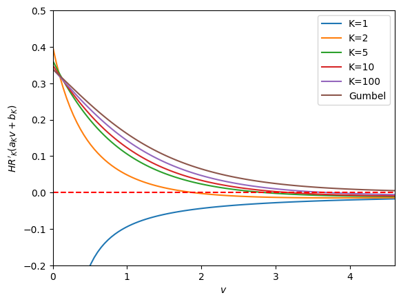
(b) Derivative of the Hazard Rate

Figure 1: The behavior of the distribution of the normalized largest order statistic ($a_{K}v+b_{K}$) when the value distribution is the Weibull distribution with shape parameter $0.9$. The sequence $(a_{K},b_{K})$ is shown in Appendix B.1.

To illustrate the behavior of the distribution of the largest order statistic, suppose that there are $K$ objects and an agent’s value for each good $v_{k}$ follows the Weibull distribution with shape parameter $0.9$, i.e., $G(v_{k})=1-\exp(-{v_{k}}^{-0.9})$. The Weibull distribution has a DHR whenever its shape parameter is smaller than one; thus, when goods are homogeneous and agents’ types are single-dimensional (i.e., $K=1$), full screening is efficient. However, if there are $K\geq 2$ goods whose value follows the same distribution i.i.d., then the distribution of the largest order statistic, $v=\max\{v_{1},\dots,v_{K}\}$, no longer has a DHR. As illustrated in Figure 1, even with $K=2$, the distribution of $v$ has an IHR for a substantially large region of $v$, and the region expands as the variety of goods $K$ increases. In the limit of $K\to\infty$, the distribution converges to the Gumbel distribution, which has an IHR for all $v\in[0,+\infty)$, implying the optimality of a no-screening mechanism in the limit of $K\to\infty$. We also note that, even with $K=2$, no screening substantially outperforms full screening (see Appendix B.1).

We further exploit the extreme value theory to analyze the limit as the number of object types approaches infinity. When there are $K$ types of different objects, an agent’s value in the reduced environment follows the largest order statistic of $K$ samples from a marginal value distribution. The classic extreme value theorem (Fisher and Tippett, 1928; Gnedenko, 1943) shows that the largest order statistic after proper renormalization can only converge in distribution to one of the three distribution families: the Gumbel, Fréchet, or reverse-Weibull distributions. For example, in the example illustrated as Figure 1, the distribution of the normalized maximum, $a_{K}v+b_{K}$, converges to Gumbel as $K\to\infty$. The limiting distribution can be reverse-Weibull only when the marginal value distribution has bounded support, with which the residual surplus of no screening trivially approaches the first best and that of full screening goes to zero. With unbounded support, the limiting distribution is determined solely by the property of the upper tail, and roughly speaking, (i) if the tail of the marginal value distribution is exponentially bounded, the limiting distribution is Gumbel, and (ii) if the marginal value distribution is heavy-tailed. In case (i), as Gumbel has an IHR, the results of Hartline and Roughgarden (2008) imply that no screening is efficient. In case (ii), Fréchet has an increasing and decreasing hazard rate (IDHR), i.e., it has an IHR if a value is smaller than a threshold and has a DHR otherwise. In this case, the efficient mechanism in the limit is characterized by the scarcity of the goods and the shape parameter of Fréchet. We demonstrate that, under a wide range of parameters, an efficient mechanism distributes goods to most people in the same manner as a no-screening mechanism, while it may reserve an option for only a few agents with exceptionally large values to endure substantial effort costs to ensure receipt of the goods. To our knowledge, this is the first paper to utilize extreme value theory for mechanism design.

While our formal theoretical analysis mostly concentrates on a stylized environment, we also discuss the implication of our results to broader environments. When some objects are commonly more valuable than others (between-agent correlation), agents are more willing to pay effort costs while the common value component benefits all users. Thus, SD performs even better. Conversely, we can also consider an environment where some agents have high valuations for all goods and others do not (within-agent correlation). As the homogeneous-good environment studied by Hartline and Roughgarden (2008) is an extreme case of this, we expect that the results should be intermediate between the homogeneous-good case and the multiple-good case.

We also investigate efficient mechanisms for broader continuous markets with multiple objects. First, we numerically compute social welfare achieved by no-screening and full-screening mechanisms for the cases of finite object types. We confirm that even when the marginal value distribution has a DHR, the performance of a no-screening mechanism improves quickly as the variety increases. Second, exploiting the property of the continuous market, we establish a linear program for deriving an efficient mechanism with general value distributions, beyond the simple i.i.d. environments, e.g., the cases of correlated values. Third, we investigate the case of asymmetric capacities. Whereas the structure of the efficient mechanism may be complicated and there is another no-screening mechanism that outperforms SD, the performance difference is relatively small. These results suggest that the insight of the theoretical analysis not only applies to the limit but also to practical situations.

We then study the automated mechanism design of an efficient mechanism for the cases of finitely many objects, which is known as a challenging task in a multi-dimensional environment with multiple objects. Nevertheless, we solve it by adopting a deep-learning approach for the automated design of a revenue-maximizing auction proposed by Dütting et al. (2019). Consistent with the theoretical and numerical analyses of the continuous market, our program often finds SD efficient even when the marginal value distribution has a DHR. This outcome suggests that the analytical assumption of the theoretical model, where each object type has a large capacity and can be approximated as a continuum, does not play a crucial role in the implication that no-screening mechanisms like SD improve in performance as the variety of goods increases.

Finally, we discuss the implication of this paper’s finding to the distribution of the pandemic vaccines against COVID-19 and other infectious diseases that may become prevalent in the future. During the COVID-19 pandemic, many authorities distributed reservation slots on an FCFS basis, with which agents can increase the probability of being assigned by enduring the costs of arriving early. Indeed, a rush to make reservations immediately after the opening was observed in many countries. It has also been reported that people were stressed because they could not make reservations without wasting much effort. In contrast, some countries adopted a mechanism that is essentially SD with an exogenous priority order and prevented this crisis preemptively. Among several different implementations of SD, we discuss how the register-invite-book system (RIB) adopted by several authorities including British Columbia and Singapore can efficiently allocate reservation slots.

2 Related Literature

The maximization of residual surplus studied in this paper is analogous to designing mechanisms with monetary transfers, such as auctions, that aim to maximize social welfare while assuming any money paid by agents is discarded. Hence, this issue is also referred to as the problem of money burning. Efficient money-burning mechanisms for agents with single-dimensional types have been characterized by Hartline and Roughgarden (2008); Yoon (2011); Condorelli (2012); Chakravarty and Kaplan (2013). These studies adopt Myerson’s (1981) approach, originally established for revenue maximization, to derive optimal solutions.

In contrast, characterizing optimal mechanisms in a setting with multiple objects and multi-dimensional types is known to be challenging. Despite revenue maximization being an important issue that many researchers have tackled (e.g., Manelli and Vincent, 2006; Pavlov, 2011; Haghpanah and Hartline, 2021; Giannakopoulos and Koutsoupias, 2018; Daskalakis et al., 2015), no complete characterization has been derived even for simple scenarios involving just two bidders and two items. Moreover, the extant partial characterization has revealed that the form of revenue-maximizing auctions varies significantly depending on specific situational details.

The literature has also shown that maximizing the residual surplus in a multi-object environment is as challenging as maximizing the revenue. Fotakis et al. (2016); Goldner and Lundy (2024) have proposed approximation mechanisms that provide certain performance guarantees, yet these do not lead to optimal solutions in general domains. The matching theory literature has also characterized efficient ordinal mechanisms (Bogomolnaia and Moulin, 2001; Che and Kojima, 2010; Liu and Pycia, 2016; Ashlagi and Shi, 2016) and applied the insights to practical applications such as school choice (Abdulkadiroğlu and Sönmez, 2003; Abdulkadiroğlu et al., 2009). However, it remains unknown whether and under which conditions ordinal mechanisms, which are no-screening mechanisms in the sense that they do not require money burning, can perform better than screening mechanisms. To address this challenge, we utilized extreme value theory to fully characterize the efficient mechanism in the large market limit under certain conditions.

Efforts have also been made to numerically maximize revenue with multi-dimensional types. Pioneering studies in the literature of automated mechanism design, such as Sandholm (2003); Conitzer and Sandholm (2004), utilize linear programming to derive an optimal mechanism. More recently, Dütting et al. (2019) addressed scalability issues by incorporating methods from deep learning, significantly enhancing the efficiency of exploring revenue-maximizing mechanisms in multi-object settings. To our knowledge, our study is the first to analyze residual surplus maximization using the automated mechanism design approach.

Previous research has established that SD, a typical implementation of the no-screening mechanism, possesses various advantageous properties, including the ones abstracted away from the model considered in this paper. Pycia and Troyan (2024) demonstrate that the random serial dictatorship in sequential form is the only mechanism that satisfies Pareto efficiency, symmetry, and obvious strategy-proofness (Li, 2017). Bade (2015) shows that SD in sequential form is the only ordinally efficient and group strategy-proof mechanism when agents can endogenously acquire information about their preferences, and Hakimov et al. (2023) empirically confirm that this effect is substantial in a school choice problem. Krysta et al. (2014) prove that random serial dictatorship achieves at least $1-1/e\>(\approx 63.2\%)$ of the first-best matching size (which corresponds to the total number of vaccines administered in the vaccine application), and Noda (2020) shows that no strategy-proof mechanism has a better worst-case guarantee. Hakimov et al. (2021) further demonstrate that SD can prevent market functionality from being compromised by scalpers. In addition to these properties, this paper demonstrates that SD achieves high social welfare (residual surplus) when many heterogeneous objects are distributed. Considering these results, SD is well-suited for allocating many heterogeneous goods like reservation slots for vaccines.

Finally, research on the allocation and supply of medical resources during public health crises like the COVID-19 pandemic has been rapidly increasing in recent years. Ahuja et al. (2021); Castillo et al. (2021); Athey et al. (2022) analyze how to incentivize pharmaceutical companies to invest in production capacity, thereby accelerating vaccine supply. Noda (2018) proposes a matching mechanism to maximize the vaccination rate when authorities can design the capacity of vaccination sites. Gans (2022) and Akbarpour et al. (2023) study optimal vaccination priorities based on the private and social benefits. Pathak et al. (2022, 2024) design a reserve system to fairly allocate scarce medical resources. These studies have contributed to the optimization of the upstream segments of the massive undertaking of vaccine production, distribution, and allocation. In contrast, our paper focuses on the downstream segment, enhancing the efficiency of the vaccine distribution process by determining when and at which vaccination site individuals should receive their vaccines.

3 Continuous Market

3.1 Model

We first consider a continous market with a unit mass of a continuum of agents $I\coloneqq[0,1]$ with a unit demand. Each object has a type $k\in K$. We assume that $K$ is a finite set. The set of object types $K$ is assumed to be finite, and the mass of type-$k$ objects is denoted by $m_{k}\in\mathbb{R}_{+}$. We denote the total mass of objects by $\bar{m}\coloneqq\sum_{k\in K}m_{k}$.

Each agent is specified by their valuation vector, $\mathbf{v}=(v_{k})_{k\in K}\in V\subset\mathbb{R}_{+}^{K}$, where $v_{k}$ denotes this agent’s valuation for a type-$k$ object. For notational simplicity, we omit the index specifying the agent’s identity; thus, $\mathbf{v}$ represents the valuation vector of a single agent, not their profile. Agents can choose the level of effort costs, and the central planner can observe it. Since efforts are used just like payments, we refer to them simply as “payments” in this paper, whereas we emphasize that all payments are burned without enriching the central planner as revenue. We assume that agents have a quasi-linear utility function. Accordingly, when this agent obtains object $k$ with probability $x_{k}\in[0,1]$ for each $k$ while making a payment of $p$, her payoff is

$$\sum_{k\in K}v_{k}x_{k}-p.$$ (1)

Throughout this section, we consider direct mechanisms that determine an allocation and payment based only on the agent’s own report and the distribution of the reported type profiles. This restriction has two effects. First, we can drop an index representing the agent’s identity because an agent’s identity does not alter the agent’s outcome. Second, in a continuous market, there is no aggregate uncertainty, and thus if a mechanism satisfies an appropriate incentive compatibility condition, the distribution of reported types remains constant in equilibrium. Accordingly, we can also omit the other agents’ type reports from arguments of the mechanism. A mechanism $\mathcal{M}$ is comprised of an allocation rule $\mathbf{x}:V\to[0,1]^{K}$ and a payment rule $p:V\to\mathbb{R}_{+}$, where $\mathbf{x}(\mathbf{v})$ and $p(\mathbf{v})$ are the respective allocation and payment when the agent has a valuation $\mathbf{v}$. Let $F:V\to[0,1]$ be the cumulative distribution function of agents’ valuations. Our main measure of social welfare, residual surplus from a mechanism $\mathcal{M}=(\mathbf{x},p)$ is defined as

$$RS(\mathcal{M})\coloneqq\int_{V}\left(\sum_{k\in K}v_{k}x_{k}(\mathbf{v})-p(\mathbf{v})\right)dF(\mathbf{v}).$$ (2)

In our setting, because payments are burned, the objective function (2) differs from the gross surplus, social welfare considered in a setting with monetary transfers:

$$GS(x)\coloneqq\int_{V}\sum_{k\in K}v_{k}x_{k}(\mathbf{v})dF(\mathbf{v}).$$ (3)

An allocation rule $\mathbf{x}$ is allocatively efficient if it maximizes the gross surplus.

Below, we list several constraints a mechanism must satisfy. A mechanism $\mathcal{M}$ satisfies the resource constraint if, for each $k$, there is at most mass $m_{k}$ of agents who receive object $k$.

$$\int_{V}x_{k}(\mathbf{v})dF(\mathbf{v})\leq m_{k}\text{ for all }k\in K.$$ (4)

A mechanism $\mathcal{M}$ is strategy-proof if no agent obtains a higher payoff by pretending to have another valuation:

$$\sum_{k\in K}v_{k}x_{k}(\mathbf{v})-p(\mathbf{v})\geq\sum_{k\in K}v_{k}x_{k}(\mathbf{v}^{\prime})-p(\mathbf{v}^{\prime})\text{ for all }\mathbf{v},\mathbf{v}^{\prime}\in V.$$ (5)

A mechanism $\mathcal{M}$ is individually rational if no agent obtains a negative payoff:

$$\sum_{k\in K}v_{k}x_{k}(\mathbf{v})-p(\mathbf{v})\geq 0\text{ for all }\mathbf{v}\in V.$$ (6)

A mechanism $\mathcal{M}$ satisfies the unit demand condition if an agent obtains at most one object in expectation.

$$\sum_{k\in K}x_{k}(\mathbf{v})\leq 1\text{ for all }\mathbf{v}\in V.$$ (7)

A mechanism $\mathcal{M}$ is efficient if it maximizes the residual surplus $RS$ subject to all the above constraints, (4), (5), (6), and (7).

3.2 Theoretical Analysis

3.2.1 I.I.D. Environment

In this section, we derive a closed-form characterization of an efficient mechanism. It is well-known that characterizing mechanisms that optimize objectives such as revenue or agents’ welfare in a money-burning setting is an extremely challenging task when agents have multi-dimensional private information. Therefore, we make several additional simplifying assumptions to enable theoretical analysis within this section. We then utilize numerical computations to examine the extent to which our findings can apply to more practical settings.

Specifically, we assume that the set of all possible valuations $V$ can be written as a $V=[0,\bar{v}]^{K}$, where $\bar{v}\in\mathbb{R}\cup\{+\infty\}$, and there exists a marginal value distribution $G:[0,\bar{v}]\to[0,1]$ such that the distribution function of valuation vectors, $F$, can be written as a product of the $G$ function: For all $\mathbf{v}=(v_{k})_{k\in K}$, we have $F(\mathbf{v})=\prod_{k\in K}G(v_{k})$. That is, each valuation for object $k$, $v_{k}$, follows $G$ i.i.d. Throughout this paper, we assume that $G$ has full support and $G$ is twice continuously differentiable. The first and second-order derivative of $G$ is written as $g$ and $g^{\prime}$, respectively. We further assume that all object types have the same capacity; i.e., we set $m_{k}=\bar{m}/K$ for all objects $k\in K$. We focus on the case of $\bar{m}<1$ to make the problem non-trivial. We refer to this environment as an i.i.d. environment. As we assume all object types are symmetric, an i.i.d. environment is parametrized by its marginal value distribution $G$ and the cardinality of object types, $|K|$. Slightly abusing notation, we denote $K$ to represent its cardinality $|K|$ unless it causes confusion.

3.2.2 Reduction to a Single-Dimensional Environment

To facilitate our analysis, we additionally impose two conditions on the mechanisms: object symmetry and ex post efficiency. We say that a mechanism is object-symmetric if it treats all objects symmetrically, without using their a priori labels.

Definition 1 (Object-Symmetry).

A mechanism $\mathcal{M}=(\mathbf{x},p)$ is object-symmetric if for all permutation of objects $\sigma:K\to K$, we have

$$\mathbf{x}(\sigma(\mathbf{v})) =\sigma(\mathbf{x}(\mathbf{v})),$$ (8)

$$p(\sigma(\mathbf{v})) =p(\mathbf{v}).$$ (9)

In the i.i.d. environment considered in this section, all objects are symmetric, thus it is natural to focus on object-symmetric mechanisms. The assumption of object-symmetry is innocuous by itself in the sense that any i.i.d. environment has an efficient and object-symmetric mechanism.

Proposition 1.

In an i.i.d. environment, there exists an efficient and object-symmetric mechanism.

The proof is similar to that of Theorem 1 of Rahme et al. (2021).

We say that a mechanism is ex post (Pareto) efficient if the allocation resulting from the mechanism satisfies the property that no group of agents can simply exchange objects without monetary transfers and still make a mutual gain.

Definition 2 (Ex Post Efficiency).

An allocation rule $x$ is ex post efficient if there is no allocation rule $x^{\prime}$ that satisfies the following four conditions: (i) the resource constraint, (ii) the unit demand condition, (iii) $\sum_{k\in K}v_{k}x^{\prime}_{k}(\mathbf{v})\geq\sum_{k\in K}v_{k}x_{k}(\mathbf{v})$ for all $\mathbf{v}\in V$, and (iv) there exists $V^{\prime}\subset V$ such that $F(V^{\prime})>0$ and $\sum_{k\in K}v_{k}x^{\prime}_{k}(\mathbf{v})>\sum_{k\in K}v_{k}x_{k}(\mathbf{v})$ for all $\mathbf{v}\in V^{\prime}$.

Ex post efficiency is clearly a necessary condition for a mechanism to maximize the gross surplus in a broad range of environments. Whereas it is not immediately clear whether ex post efficiency is also a necessary condition for the residual-surplus maximization, ex post efficiency, which guarantees no incentive to simply exchange objects allocated, is in itself a desirable property in practice. Therefore, we impose this condition as a constraint that mechanisms must satisfy, and leverage it in our theoretical analysis.

To achieve ex post efficiency, we should allocate objects in such a way that agents receive their favorite one whenever possible. In an i.i.d. environment, the scarcity of all objects is equal, and object-symmetry requires the mechanism to allocate objects in a symmetric manner. Accordingly, it is indeed feasible to assign every agent their favorite one whenever they are allocated. Consequently, under a mechanism that is both object-symmetric and ex post efficient, each agent faces only two possibilities: receiving their favorite objects or receiving nothing at all.

Theorem 1.

In a continuous i.i.d. environment, if $\mathcal{M}=(x,p)$ is object-symmetric and ex post efficient, then there exists $V^{\prime}\subset V$ such that $F(V^{\prime})=1$ and $x_{k}(\mathbf{v})>0$ implies $v_{k}=\max_{l\in K}v_{l}$ for all $\mathbf{v}\in V^{\prime}$.

Proofs are shown in Appendix A. Due to Theorem 1, since each agent can only obtain their favorite object, valuations for other objects can be disregarded. Thus, the problem can be reduced to a simpler environment with single-dimensional types. We denote each agent’s valuation for the “single object” in the reduced environment as $v$, and let $G_{K}$ be its distribution. The value $v$ is defined as the largest order statistic of valuations in the original environment: $v\coloneqq\max_{k\in K}v_{k}$. Thus, we can derive its distribution $G_{K}$ using the marginal value distribution $G$ as $G_{K}(v)\coloneqq(G(v))^{K}$. We refer to $G_{K}$ as the reduced value distribution. Slightly abusing the notation, we use $(x,p)$ to represent the allocation rule and the payment rule, whereas now $x:[0,\bar{v}]\to[0,1]$ and $p:[0,\bar{v}]\to\mathbb{R}$ maps each agent’s value for the favorite object $v$ to the probability that she obtains her favorite good $x(v)$ and her payment $p(v)$, respectively.

The reduced problem is expressed as follows.

$$\max_{(x,p)}\int_{0}^{\infty}\left(vx(v)-p(v)\right)dG_{K}(v)$$ (10)

s.t. $$\int_{0}^{\bar{v}}x(v)dG_{K}(v)=\bar{m}\text{ for all }w\in[0,\bar{v}],$$ (Resource Constraint)

$$vx(v)-p(v)\geq vx(v^{\prime})-p(v^{\prime})\text{ for all }v,v^{\prime}\in[0,\bar{v}],$$ (Strategy-Proofness)

$$vx(v)-p(v)\geq 0\text{ for all }v\in[0,\bar{v}],$$ (Individual Rationality)

$$x(v)\leq 1\text{ for all }v\in[0,\bar{v}].$$ (Unit Demand)

3.2.3 Mechanisms

No Screening and Serial Dictatorship

For a reduced environment, a no-screening mechanism is defined as a mechanism that randomly assigns $\bar{m}$ units of the right to obtain the most preferred object to one unit of agents, regardless of their (reduced) value $v$. That is, $x(v)=\bar{m}$ and $p(v)=0$ for all $v\in[0,\bar{v}]$. This result is achieved in an i.i.d. environment if we apply serial dictatorship (SD), in which agents take their most preferred objects sequentially following a priority order. The residual surplus achieved under SD is

$$RS(\mathcal{M}_{SD})=\bar{m}\int_{0}^{\bar{v}}vdG_{K}(v).$$ (12)

Note that, besides SD, various no-screening mechanisms (e.g., the random favorite mechanism discussed in Section 3.3.2) yield an equivalent reduced mechanism to SD in an i.i.d. environment.

Full Screening and VCG

For a reduced environment, a full-screening mechanism is defined as a mechanism that, even at the cost of screening, identifies agents’ values to achieve allocative efficiency. In the reduced environment, the allocatively efficient allocation rule is to assign the right to obtain the most preferred object with probability $1$ to the agents with the highest value for a mass $\bar{m}$ units, while not allocating the good to any other agents; i.e., $x(v)=1$ if $v\geq q$ and $x(v)=0$ otherwise, where $q\in[0,\bar{v}]$ is the $(1-\bar{m})$-quantile of the reduced value distribution $G_{K}$: $1-G_{K}(q)=\bar{m}$. To implement this allocation rule, in a continuous i.i.d. environment, the mechanism should require paying a price of $q$ for allocated agents. The residual surplus achieved under VCG is

$$RS(\mathcal{M}_{VCG})=\int_{q}^{\bar{v}}\left(v-q\right)dG_{K}(v).$$ (13)

For general environments, including finite environments and continuous but non-i.i.d. environments, the Vickrey-Clarke-Groves mechanism (VCG), which requires each agent to pay their externality, achieves allocative efficiency. Furthermore, the revenue equivalence theorem of Myerson (1981) shows that VCG is the unique direct mechanism for achieving allocative efficiency in single-dimensional environments.

Unlike purely artificial mechanism designs such as auctions, direct mechanisms, including VCG, are not practically used in screening mechanisms utilizing ordeals. However, when indirect mechanisms are employed, the resulting equilibrium allocations often coincide with those achieved by direct mechanisms. For example, FCFS is analogous to an all-pay auction in the sense that (i) those who exert more effort and arrive first obtain the goods, and (ii) the effort cost is incurred even if the good is not secured. In a single-dimensional environment, an all-pay auction has an equilibrium where the good is allocated to the mass $\bar{m}$ of agents with the highest value, and the expected payment in this equilibrium matches that of VCG. Although it is uncertain whether similar results hold in general multi-object environments, even in such cases, VCG remains a useful benchmark for mechanisms that involve screening.

3.2.4 Characterizations for the Single-Dimensional Environment

Hartline and Roughgarden (2008) analyzes a money-burning problem with single-dimensional environments, applying the Myersonean approach originally established for revenue maximization (Myerson, 1981). We review their results to present our characterization for a continuous i.i.d. environment. Note that, while Myerson (1981) and Hartline and Roughgarden (2008) state all the characterization results under Bayesian incentive compatibility (BIC), we replace BIC with strategy-proofness because these two incentive constraints are equivalent in a continuous environment.

Myerson (1981) proves that (i) an allocation rule can comprise a strategy-proof mechanism if and only if $x$ is monotonic (i.e., $x(v^{\prime})\geq x(v)$ for all $v^{\prime}\geq v$), and (ii) if an allocation is nondecreasing, strategy-proofness uniquely identifies the payment rule (up to constant). Using this approach, Hartline and Roughgarden (2008) show that expected social welfare is equal to the expectation of the virtual valuation for utility $\vartheta$ under strategy-proofness (see their Lemma 2.6):

$$\mathbb{E}[vx(v)-p(v)]=\int_{0}^{\bar{v}}\left(vx(v)-p(v)\right)dG_{K}(v)=\int_{0}^{\bar{v}}\vartheta(v;G_{K})x(v)dG_{K}(v)=\mathbb{E}[\vartheta(v;G_{K})x(v)].$$ (14)

where

$$\vartheta(v;G_{K})\coloneqq\frac{1-G_{K}(v)}{g_{K}(v)}.$$ (15)

In the context of revenue maximization, we exploit the relation of $\mathbb{E}[p(v)]=\mathbb{E}[(v-\vartheta(v;G_{K}))x(v)]$ to characterize an optimal mechanism. The value, $v-\vartheta(v;G_{K})$, is defined as the virtual valuation for payment. Since this paper’s focus is on residual-surplus maximization, we rather refer to $\vartheta(v;G_{K})$ as the virtual valuation (for residual surplus).

Note also that $r(v;G)=1/\vartheta(v;G)=g(v)/(1-G(v))$ is called the hazard rate function of the distribution $G$. We say that a distribution $G$ has an increasing hazard rate (IHR) if $r(\cdot;G)$ is nondecreasing. Conversely, $G$ has a decreasing hazard rate (DHR) if $r(\cdot;G)$ is nonincreasing.

Given the characterization above, the problem reduces to the maximization of $\mathbb{E}[\vartheta(v)x(v)]$ subject to the resource constraint, individual rationality, the unit demand condition, and monotonicity of $x$. If the reduced value distribution $G_{K}$ has a DHR, the monotonicity constraint is unbinding, and an efficient mechanism maximizes the value of $x(v)$ in regions where $v$ is larger, while fulfilling the resource constraint and the unit demand condition, which is precisely a full-screening mechanism. Conversely, if $G_{K}$ has an IHR, the monotonicity constraint is binding for every $v$, and therefore, a no-screening mechanism adopting $x(v)\equiv\bar{m}$ is efficient.

Theorem 2.

In a continuous i.i.d. environment $(G,K)$,

1. If the reduced value distribution $G_{K}$ has an IHR, then a no-screening mechanism is efficient.

2. If $G_{K}$ has a DHR, then a full-screening mechanism is efficient.

Theorem 2 is immediate from Corollary 2.11 and 2.12 of Hartline and Roughgarden (2008), given that the residual-surplus maximization problem in a continuous i.i.d. market can be reduced to the problem in a single-dimensional environment with the value distribution $G_{K}$.

The behavior of the hazard rate is closely related to the tail weight of the value distribution. Under the exponential distribution, $G_{K}(v)=1-e^{-\lambda v}$ for all $v\geq 0$ where $\lambda>0$ is a parameter, the hazard rate (and thus the virtual valuation) is constant. Thus, both no- and full-screening mechanisms are efficient and these two mechanisms lead to identical residual surplus. IHR and DHR imply that the tail of the value distribution is lighter and heavier than the exponential distribution. As the tail becomes heavier, the benefit of screening for agents with very high valuations increases.

Finally, if the reduced value distribution satisfies neither IHR nor DHR properties, an efficient mechanism can be obtained through a procedure called “ironing,” proposed by Myerson (1981).

3.2.5 Hazard Rate Property

This section discusses how the hazard rate function $r(\cdot;G_{K})$ of the reduced value distribution $G_{K}$ changes as the variety of objects, $K$, increases. Even when the marginal value distribution $G$ has a DHR, the distribution of the largest order statistic $G_{K}$ may not have a DHR. Weibull with parameter $\alpha<1$ is an example, as illustrated in Figure 1.

The following theorem conversely proves that as the variety of objects increases, the region in which the reduced value distribution has an IHR expands.

Theorem 3.

Let $r^{\prime}(\cdot;G_{K})$ be the derivative of $r(\cdot;G_{K})$ with respect to $v$. Then, $r^{\prime}(v;G_{K+1})\geq 0$ if $r^{\prime}(v;G_{K})\geq 0$. Furthermore, for all $v\in[0,\bar{v}]$, there exists $K_{0}$ such that for all $K>K_{0}$, $r^{\prime}(v;G_{K})>0$.

One useful implication immediately arises as corollaries from Theorem 3: it ensures that, if the reduced value distribution $G_{K}$ has an IHR (for all $v\in[0,\bar{v}]$) for some $K$, then for all $K^{\prime}>K$, $G_{K^{\prime}}$ also has an IHR.

Corollary 1.

In an i.i.d. environment with a marginal value distribution $G$, if $G_{K}$ has an IHR, then for all $K^{\prime}>K$, $G_{K^{\prime}}$ also has an IHR. In particular, if $G$ itself has an IHR, then for all $K\geq 1$, $G_{K}$ has an IHR.

Roughly speaking, Theorem 3 and Corollary 1 imply that, as the variety of objects $K$ increases, the reduced value distribution $G_{K}$ (i) is more likely to have an IHR, and (ii) cannot have a DHR for all $v\in[0,\bar{v}]$. As discussed in Section 3.2.4, the hazard rate property plays a critical role in characterizing efficient mechanisms, making this a significant finding.

However, it is important to note that Theorem 3 does not guarantee that a no-screening mechanism becomes efficient for sufficiently large $K$ with arbitrary marginal value distribution $G$. When the marginal value distribution is unbounded (i.e., $\bar{v}=+\infty$), the region where the reduced value distribution $G_{K}$ carries most of its probability weight shifts upward without bound as $K$ increases. While Theorem 3 ensures that the hazard rate becomes increasing around a fixed value $v$ for sufficiently large $K$, the probability of such $v$ occurring might be almost equal to zero for such large $K$. In such a case, the design of $x(v)$ and $p(v)$ around such fixed $v$ may have little impact on the overall performance of the mechanism. Accordingly, cases not covered by Corollary 1 require separate asymptotic analysis.

3.2.6 Extreme Value Theory

This section discusses the large-market results based on the asymptotic properties of the reduced value distribution $G_{K}$ in the limit of $K\to\infty$. The limiting behavior of the largest order statistic has been extensively analyzed in the literature of extreme value theory. We utilize these results to characterize efficient mechanisms in the large-market limit.

When the number of object types $K$ becomes sufficiently large, the shape of the reduced value distribution $G_{K}$ becomes less dependent on the shape of the marginal value distribution, $G$. Consequently, the limit distribution can only be either Gumbel, Fréchet, or reverse-Weibull distribution.

Definition 3.

Let $G$, $H$ be distribution functions. We say that $H$ is an extreme value distribution and that $G$ lies in its domain of attraction of $H$ if $G$ and $H$ are nondegenerate and there exist a sequence of constants $(a_{K},b_{K})_{K=1}^{\infty}$ with $a_{K}>0$ for all $K$, such that $\hat{G}_{K}(w)\coloneqq G_{K}(a_{K}w+b_{K})\to H(w)$ as $K\to\infty$ for all $w$ at which $G$ is continuous.

For notational simplicity, we define a normalized reduced value distribution $\hat{G}_{K}$ and allocation rule $\hat{x}$ as $\hat{G}_{K}(w)\coloneqq G_{K}(a_{K}w+b_{K})$ and $\hat{x}(w)\coloneqq x(a_{K}w+b_{K})$. Since $a_{K}>0$, the residual surplus maximization for $\hat{G}_{K}$ is equivalent to that for $G_{K}$. When $G$ belongs to the domain of attraction of $H$, then $\hat{G}_{K}(w)\to H(w)$.

Proposition 2 (Fisher and Tippett (1928); Gnedenko (1943)).

Only the Gumbel distribution, the Fréchet distribution, and the reverse-Weibull distribution can be an extreme value distribution, where these distributions are given by

$$\Lambda(w) =\exp(-\exp(w)),\hskip 9.00002pt-\infty<w<\infty$$ (Gumbel)

$$\Phi_{\alpha}(w) =\exp(-w^{-\alpha}),\hskip 9.00002ptw\geq 0,\alpha>0$$ (Fréchet)

$$\Psi_{\alpha}(w) =\begin{cases}\exp(-(-w)^{\alpha})&w<0\\ 1&w\geq 1\end{cases},\hskip 9.00002pt\alpha>0.$$ (reverse-Weibull)

For the proof of Proposition 2, please refer to Theorems 1.1.3 and 1.1.6 of De Haan and Ferreira (2006). Theorem 1.1.6 of De Haan and Ferreira (2006) additionally implies that, whenever a distribution function $G$ belongs to the domain of attraction of Gumbel, $\hat{G}_{K}(w)\coloneqq G_{K}(a_{K}w+b_{K})\to\Lambda(w)$ with

$$a_{K}=s(G^{-1}(1-1/K)),\>b_{K}=G^{-1}(1-1/K)$$ (16)

where

$$s(v)=\frac{\int_{v}^{\bar{v}}(1-G(v^{\prime}))dv^{\prime}}{1-G(v)}.$$ (17)

Whenever a distribution function $G$ belongs to the domain of attraction of Fréchet with shape parameter $\alpha$, $\hat{G}_{K}(w)\coloneqq G_{K}(a_{K}w+b_{K})\to\Phi_{\alpha}(w)$ with

$$a_{K}=G^{-1}(1-1/K),\>b_{K}=0$$ (18)

Throughout the paper, when we refer to $(a_{K},b_{K})_{K=1}^{\infty}$, these constants are defined by (16) or (18).

We omit the condition for reverse-Weibull because the convergence occurs only if $\bar{v}<+\infty$ and for such a case, we do not need extreme value theory for characterizing an efficient mechanism in the limit (see Theorem 4).

Proposition 2 does not state that the distribution of the normalized maximum does converge. Nevertheless, it is also known that many continuous distribution functions have an extreme value distribution. Table 1 lists extreme value distributions of common probability distributions. The limit is identical as long as distributions have the same right-tail property, even when their overall shape differs significantly.

Table 1: Extreme Value Distributions of Common Probability Distributions

Limit	Marginal Value Distribution
Gumbel	Exponential, Normal, Gamma, Log-Normal, Logistic, Weibull, Gumbel, etc.
Fréchet	Pareto, Cauchy, $t$, $F$, Burr, Log-Gamma, Zipfianm, Fréchet, etc.
Reverse-Weibull	Uniform, Beta, Reverse-Weibull, etc. (Unimportant for our analysis)

The extreme value theory literature has also characterized the conditions under which a marginal value distribution $G$ belongs to the domain of attraction of each extreme value distribution. However, this paper focuses not on the convergence of distribution functions, but on the changes in hazard rates, namely the convergence of their derivatives:

$$r^{\prime}(w;\hat{G}_{K})=\frac{\hat{g}^{\prime}_{K}(w)(1-\hat{G}_{K}(w))+(\hat{g}_{K}(w))^{2}}{\left(1-\hat{G}_{K}(w)\right)^{2}}.$$ (19)

For convergence of $r^{\prime}(\cdot;\hat{G}_{K})$, we also need a convergence of $\hat{g}_{K}$ and $\hat{g}^{\prime}_{K}$, which are the first and second derivatives of $\hat{G}_{K}$. The following is the necessary and sufficient condition for $\hat{G}_{K}$, $\hat{g}_{K}$, and $\hat{g}^{\prime}_{K}$ to converge.

Definition 4.

Let $G$ and $H$ be distribution functions. We say that $G$ lies in the twice differentiable domain of attraction of $H$ if $G$ and $H$ are nondegenerate and twice differentiable for all sufficiently large $w$ and $\hat{G}_{K}^{(l)}(w)\to H^{(l)}(w)$ as $K\to\infty$ uniformly for all $w$ in any finite interval for all $l=0,1,2$.

Definition 5 (von Mises condition).

A distribution function $G$ satisfies the von Mises condition with parameter $\alpha$ if $G$ is twice differentiable for all sufficiently large $v$ and

$$\vartheta^{\prime}(v;G)=\left(\frac{1-G(v)}{g(v)}\right)^{\prime}\to\gamma\text{ as }K\to\infty.$$ (20)

We denote the set of all distribution functions satisfying (20) by VMC($\gamma$).

The von Mises condition (20) is originally established by von Mises (1936) as a tractable sufficient condition for convergence of a distribution function. Later, Pickands III (1986) proves that (20) is a necessary and sufficient condition for convergence of the second derivative of the distribution function.

Proposition 3 (Theorem 5.2 of Pickands III (1986)).

1. $G$ is in the twice differentiable domain of attraction of the Gumbel distribution $\Lambda$ if and only if $G\in\textbf{VMC}(0)$.

2. $G$ is in the twice differentiable domain of attraction of the Fréchet distribution with shape parameter $\alpha$, $\Phi_{\alpha}$, if and only if $G\in\textbf{VMC}(1/\alpha)$.

3.2.7 Efficient Mechanisms in the Large Market Limit

This section characterizes efficient mechanisms in a large market limit of the i.i.d. environment.

Bounded Support

We start with the case of bounded support, i.e., $\bar{v}<+\infty$. In this case, no screening is efficient with sufficiently large $K$, while full screening is conversely the worst. When $K$ is large, almost every agent has at least one good that they value close to $\bar{v}$. Therefore, even with no screening, the gross surplus approaches $\bar{v}$, and there is no need to screen the intensity of preferences. On the other hand, if screening is conducted, all the surplus is burned due to competition.

Formally, for any $\epsilon>0$ and $\delta>0$, with a sufficiently large $K$, the fraction of agents whose value for the favorite object $v$ is in $(\bar{v}-\epsilon,\bar{v}]$ is larger than $1-\delta$. For such a large $K$, the residual surplus generated by no screening is at least $\bar{m}(1-\delta)(\bar{v}-\epsilon)$, which can be arbitrarily close to the first-best value of $\bar{m}\bar{v}$, implying that no screening is approximately efficient. By contrast, the residual surplus achieved by full screening is at most $\bar{m}\epsilon$, which becomes arbitrarily close to zero.

Theorem 4.

Suppose that $\bar{v}<+\infty$. Then, for any $\epsilon>0$ and $\delta>0$, there exists $K_{0}>0$ such that for all $K>K_{0}$, we have both $RS(\mathcal{M}_{SD})>\bar{m}(1-\delta)(\bar{v}-\epsilon)$ and $RS(\mathcal{M}_{VCG})<\bar{m}\epsilon$.

Gumbel Case

Next, we consider the case where the marginal value distribution $G$ satisfies VMC(0), and thus belongs to the twice differentiable domain of attraction of the Gumbel distribution $\Lambda$. The hazard rate function of Gumbel is given by

$$r(w;\Lambda)=\frac{\lambda(w)}{1-\Lambda(w)}=\frac{\exp(-w)}{\exp(\exp(-w))-1},$$ (21)

and thus the Gumbel distribution $\Lambda$ has an IHR. Accordingly, if the reduced value distribution is exactly Gumbel, then an efficient mechanism is a no-screening mechanism.

Proposition 3 ensures that whenever $G\in\textbf{VMC}(0)$, $\hat{G}_{K}(w)$ converges to $\Lambda(w)$ up to the second derivative, uniformly in any finite interval of $w$. Accordingly, for any finite interval $[\underline{c},\bar{c}]$, the virtual valuation $\vartheta(\cdot;\hat{G}_{K})$ becomes decreasing in $[\underline{c},\bar{c}]$ with sufficiently large $K$.

Lemma 1.

If $G\in\textbf{VMC}(0)$, then for any finite interval $[\underline{c},\bar{c}]$, there exists $K_{0}$ such that for all $K>K_{0}$, we have $\vartheta^{\prime}(w;\hat{G}_{K})<0$ for $w\in[\underline{c},\bar{c}]$.

The following lemma, a well-known fact in the revenue maximization literature, ensures that an optimal allocation rule $x$ is constant for any interval $[a,b]$ where the virtual valuation $\vartheta$ is nonincreasing.

Lemma 2.

Let $[a,b]$ be an interval on which virtual valuation $\vartheta(\cdot;\hat{G}_{K})$ is nonincreasing, and $x$ be the allocation rule of any strategy-proof mechanism. Then, the allocation rule

$$\tilde{x}(w)\coloneqq\begin{cases}\dfrac{\displaystyle\int_{a}^{b}x(w^{\prime})\hat{g}_{K}(w^{\prime})dw^{\prime}}{\hat{G}_{K}(a)-\hat{G}_{K}(b)}&\text{ if }w\in[a,b]\\ x(w)&\text{otherwise}\end{cases}$$ (22)

is a monotonic allocation rule that satisfies the resource constraint. Furthermore, its residual surplus is no less than that of $x$.

Lemmas 1 and 2 immediately imply that for any interval $[\underline{c},\bar{c}]$, there exists $K_{0}$ such that for all $K>K_{0}$, an efficient allocation rule becomes constant in the interval: $\hat{x}(w)=\bar{x}$ for $w\in[\underline{c},\bar{c}]$. Furthermore, as $\hat{G}(\bar{c})-\hat{G}(\underline{c})\to\Lambda(\bar{c})-\Lambda(\underline{c})$, by taking small $\underline{c}$, large $\bar{c}$, and large $K$, we can make $\hat{G}_{K}(\bar{c})-\hat{G}_{K}(\underline{c})$ arbitrarily close to one. Since all of the $\bar{m}$ unit of goods should be allocated equally to agents with $w\in[\underline{c},\bar{c}]$, their probability of assignment also becomes arbitrarily close to $\bar{m}$. In this sense, an efficient mechanism conducts no screening asymptotically.

Theorem 5.

If $G\in\textbf{VMC}(0)$, then for all $\epsilon>0$, there exists $K_{0}$ such that for all $K>K_{0}$, an efficient allocation rule $\hat{x}$ for $(G,K)$ satisfies $\Pr(\hat{x}(w)=\bar{x})>1-\epsilon$, where $\bar{x}\in((\bar{m}-\epsilon)/(1-\epsilon),\bar{m}/(1-\epsilon))$.

Fréchet Case

Finally, we consider the case where the marginal value distribution $G$ satisfies VMC($1/\alpha$) for some $\alpha>0$, and thus belongs to the twice differentiable domain of attraction of the Fréchet distribution with shape parameter $\alpha$, $\Phi_{\alpha}$. When $\alpha\in(0,1]$, the right tail is extremely heavy, and the distribution does not have a mean; thus, we focus on the case of $\alpha>1$, where agents’ expected payoffs are well-defined. The hazard rate function of Fréchet with parameter $\alpha$ is given by

$$r(w;\Phi_{\alpha})=\frac{\phi_{\alpha}(w)}{1-\Phi_{\alpha}(w)}=\frac{\alpha w^{-\alpha-1}\exp(-w^{-\alpha})}{1-\exp(-w)^{-\alpha}}.$$ (23)

By direct calculation, we can verify that Fréchet has an IDHR, i.e., there exists $w^{*}$ such that the hazard rate is increasing for $w<w^{*}$ and it is decreasing for $w>w^{*}$.

If the reduced value distribution has neither IHR nor DHR, we need to apply Myerson’s (1981) ironing to produce the ironed virtual value $\bar{\vartheta}$. An efficient mechanism maximizes the value of $\hat{x}(w)$ in regions where $\bar{\vartheta}(w;\hat{G}_{K})$ is larger while fulfilling the resource constraint and the unit demand condition (see Theorem 2.8 of Hartline and Roughgarden, 2008). When $\hat{G}_{K}$ has an IDHR, the shape of the ironed virtual value $\bar{\vartheta}$ is relatively simple.

Lemma 3.

When the reduced value distribution $\hat{G}_{K}$ has an IDHR, the ironed virtual value $\bar{\vartheta}$ is given by

$$\bar{\vartheta}(w;\hat{G}_{K})=\begin{cases}\vartheta(w^{**};\hat{G}_{K})&\text{ for }w\in[0,w^{**}]\\ \vartheta(w;\hat{G}_{K})&\text{ for }w\in(w^{**},+\infty)\end{cases}$$ (25)

where $w^{**}$ is the solution of

$$\frac{\displaystyle\int_{0}^{w}\vartheta(w^{\prime};\hat{G}_{K})\hat{g}_{K}(w^{\prime})dw^{\prime}}{\hat{G}_{K}(v)}=\vartheta(w;\hat{G}_{K}).$$ (26)

Note that $w^{**}>w^{*}$ must be the case because when $w=w^{*}$, the left-hand side of (26) is negative while the right-hand side is zero.

Lemma 3 implies that if the reduced value distribution has an IDHR, then an efficient mechanism fully screens agents’ preferences for $w>w^{**}$, whereas conducts no screening for $w<w^{**}$. If the supply $\bar{m}$ is insufficient to allocate all agents with $w>w^{**}$, then only those with the highest values will win an item. Otherwise, an efficient mechanism first allocates goods with probability one to agents with values $w>w^{**}$. The remaining goods are then distributed equally among the other agents without requiring money burning.

Proposition 4.

When the reduced value distribution function $\hat{G}_{K}$ has an IDHR, there exists $w^{**}>w^{*}$ with which an efficient allocation rule $\hat{x}$ is represented as follows:

1. If $1-\hat{G}_{K}(w^{**})\geq\bar{m}$, then

   $$\hat{x}(w)=\begin{cases}1&\text{ for }w\in[\hat{G}_{K}^{-1}(1-\bar{m}),+\infty),\\ 0&\text{ for }w\in[0,\hat{G}_{K}^{-1}(1-\bar{m})).\end{cases}$$ (27)

2. If $1-\hat{G}_{K}(w^{**})<\bar{m}$, then

   $$\hat{x}(w)=\begin{cases}1&\text{ for }w\in[w^{**},+\infty),\\ \dfrac{\bar{m}-(1-\hat{G}_{K}(w^{**}))}{\hat{G}_{K}(v^{**})}&\text{ for }w\in[0,w^{**}).\end{cases}$$ (28)

The proof is immediate from Lemma 3.

In particular, if the value distribution is Fréchet with parameter $\alpha$, then $w^{**}$ is a solution of

$$(1-\exp(-w^{-\alpha}))w+\Gamma\left(\frac{\alpha-1}{\alpha},w^{-\alpha}\right)-\frac{1}{\alpha}w^{\alpha+1}(1-\exp(-w^{-\alpha}))=0,$$ (29)

where $\Gamma(s,x)=\int_{x}^{\infty}t^{s-1}e^{-t}dt$ is the upper incomplete gamma function.

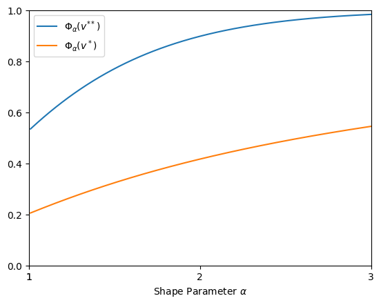
Figure 2: $\Phi_{\alpha}(w^{*})$, the size of the region where Frećhet with shape parameter $\alpha$ has an IHR, and $\Phi_{\alpha}(w^{**})$, the size of the region where the ironed virtual value is flat.

Figure 2 shows the values of $\Phi_{\alpha}(w^{*})$ and $\Phi_{\alpha}(w^{**})$ for various shape parameters $\alpha$. As $\alpha$ becomes larger, the right tail of Fréchet decays, and in the limit of $\alpha\to\infty$, the distribution converges to Gumbel. Accordingly, as $\alpha$ increases, both $\Phi_{\alpha}(w^{*})$ and $\Phi_{\alpha}(w^{**})$ increase and converge to one. Nevertheless, the convergence of $\Phi_{\alpha}(w^{*})$ is relatively slow. By contrast, the fraction of agents with $w>w^{**}$ diminishes rapidly even with relatively small $\alpha$, implying that under Fréchet with relatively small $\alpha$, an efficient mechanism conducts no screening for most agents. For example, in the case of $\alpha=3$ and $\bar{m}=0.5$, an efficient mechanism requires a substantial amount of money burning as a condition for obtaining a good with probability $1$, which only agents with the highest $1.5$% of values will choose. The remaining units, which can cover $48.5$% of the population, are distributed to the rest of $98.5$% of agents without any cost or screening, just as SD would do.

Finally, we characterize the efficient mechanism when $G\in\textbf{VMC}(1/\alpha)$ and $K$ is large but finite. The condition $G\in\textbf{VMC}(1/\alpha)$ implies that for any finite interval $[\underline{c},\bar{c}]$, if $K$ is sufficiently large, $\hat{G}_{K}$ is close to Fréchet $\Phi_{\alpha}$ within that interval. By choosing $\underline{c}$ close to zero and $\bar{c}$ larger than $w^{**}$, and accordingly taking a large $K$, the efficient allocation rule $\hat{x}$ for $\hat{G}_{K}$ becomes constant over most of the interval $[0,w^{**}]$.

Theorem 6.

If $G\in\textbf{VMC}(1/\alpha)$, then for all $\epsilon>0$, there exists $K_{0}$ such that for all $K>K_{0}$, an efficient allocation rule $\hat{x}$ for $(G,K)$ satisfies $\Pr(\hat{x}(w)=\bar{x})\in(\Phi_{\alpha}(w^{**}-\epsilon),\Phi_{\alpha}(w^{**}+\epsilon))$, where $w^{**}$ is a solution of the equation (29).

3.3 Numerical Analysis

Despite our theoretical analysis, it remains unclear what happens when the number of types of goods is finite or when the goods are asymmetric. Besides, mechanism design in multi-dimensional environments is known as a challenging task. Characterizing an efficient mechanism in non-i.i.d. environments analytically is particularly difficult. Therefore, we use a numerical approach to analyze cases that fall outside the scope of our theoretical analysis.

3.3.1 Finite Variety

We first examine whether the limit theorems provide useful insights for the case of finite object types, $K$. We numerically analyze a distribution that shifts the Pareto distribution such that the lower bound of its support becomes zero. Its distribution function is given by $G(v)=1-[(1/(v+1)]^{\alpha}$. For any $\alpha>0$, this distribution has a DHR, and thus VCG is efficient if objects are homogeneous, i.e., $K=1$. As $K\to\infty$, the distribution converges to $\Phi_{\alpha}$, Fréchet with shape parameter $\alpha$.

We investigate two scenarios. In both scenarios, $\alpha=2$, thus the limit distribution is $\Phi_{2}$. However, we assume a relatively abundant endowment in case (i), with $\bar{m}=0.6$, whereas in case (ii), we assume extreme scarcity with $\bar{m}=0.1$. If the reduced value distribution is $\Phi_{2}$, then SD outperforms VCG in case (i), while the opposite is true in case (ii).

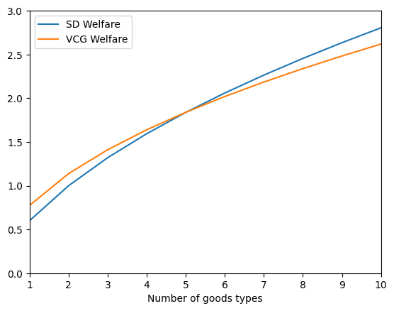
(a) Case (i): $(\bar{m},\alpha)=(0.6,2)$

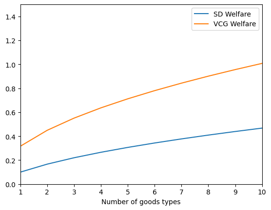
(b) Case (ii): $(\bar{m},\alpha)=(0.1,2)$

Figure 3: The residual surplus achieved by SD and VCG under Pareto distribution with finite object types.

Figure 3 plots $RS(\mathcal{M}_{SD})$ and $RS(\mathcal{M}_{VCG})$ for finite $K$ in cases (i) and (ii). In case (i), where SD performs better in the limit, the performance of SD improves rapidly, and SD outperforms VCG even with a relatively small number of object types, such as $K=5$. By contrast, in case (ii), VCG consistently performs better for all $K$ and the difference in social welfare seems monotonic in $K$. These examples suggest that our analysis of the limit could be useful for predicting what mechanisms perform well even in a practical environment with finite object types.

3.3.2 Asymmetric Capacity

In Section 3.2, for analytical tractability, we assumed that all object types have an equal capacity. This assumption is not always realistic; for example, there are only two weekend days compared to five weekdays. In such environments, an ex post efficient mechanism may assign non-favorite objects when an agent’s favorite object is scarce, making it difficult to reduce the problem to a single-dimensional environment as discussed in Section 3.2.2. This complexity makes it challenging to characterize an efficient mechanism.

In this section, we solve a linear program (LP) to numerically derive an efficient mechanism and compare its structure with that of the efficient mechanism in an i.i.d. environment. The residual surplus function $RS$ and constraints (4), (5), (6), and (7) are all linear in the allocation and payment rule, $(x,p)$, and thus this problem is an LP. To use a solver, we discretize the valuation space $V\subset\mathbb{R}^{K}$ by dividing each dimension into $n$ intervals with equal probability weights to produce $n^{K}$ grid points, each of which is specified as a $K$-tuple of lower endpoints. Throughout this paper, we take $n=40$ intervals.

We consider the case of $K=2$ and assume that the value for each object is drawn from a standard exponential distribution independently. If both objects had an equal capacity, then SD would be efficient. Here, we instead assume that $m_{1}=0.4$ and $m_{2}=0.1$.

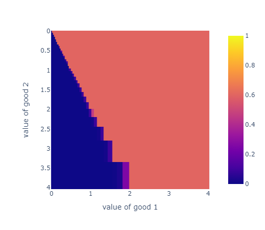
(a) $x_{1}(v_{1},v_{2})$

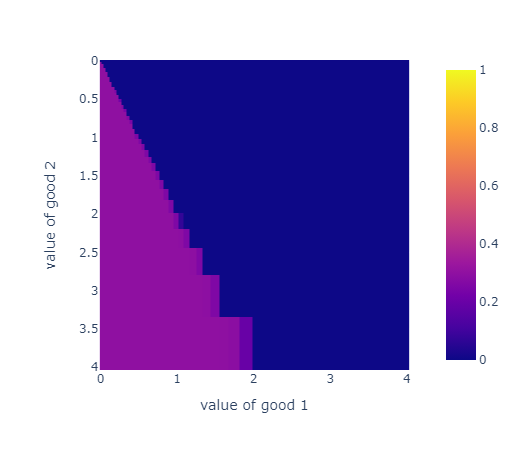
(b) $x_{2}(v_{1},v_{2})$

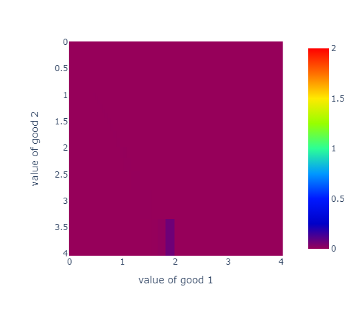
(c) $p(v_{1},v_{2})$

Figure 4: An efficient mechanism for the case of asymmetric capacity. The optimal solution can be achieved with RF.

Figure 4 illustrates an optimal solution to the LP for the case of asymmetric capacity. For all figures, the horizontal axis represents the value of object $1$ ($v_{1}$), and the vertical axis represents the value of object $2$ ($v_{2}$). The colors of panels (a), (b), and (c) indicate the probability of allocating objects $1$ and $2$ ($x_{1}(v_{1},v_{2}),x_{2}(v_{1},v_{2})$), and the payment ($p(v_{1},v_{2})$), respectively. (Figures B.9 and B.10 in Appendix B.2 show SD and VCG as an efficient mechanism in an i.i.d. environment in the same style as Figure 4.)

The efficient mechanism is neither SD nor VCG. The mechanism offers two options: Receiving object $1$ with high probability or receiving object $2$ with low probability, without requiring payments. Following the terminology of Goldner and Lundy (2024), we call this mechanism the random-favorites mechanism (RF). By requiring which object to claim before drawing a lottery, this mechanism partially screens for agents’ preference for their favorite object relative to the other one—only agents who strongly prefer object $2$ over object $1$ desire to claim object $2$, given that object $1$ is much easier to obtain. By contrast, under SD, claiming object $2$ when it is available is risk-free, and therefore, all agents who prefer object $2$ over object $1$ obtain object $2$ whenever possible. Consequently, RF outperforms SD with asymmetric capacities.

While RF outperforms SD in the residual surplus, it comes with several drawbacks. While RF can be implemented as a strategy-proof mechanism in a continuous market, to determine the allocation probability of each option, we need information about the value distribution, which is often considered challenging in the market design literature (Wilson, 1985). By contrast, SD is detail-free. Furthermore, RF cannot satisfy strategy-proofness in a finite market, even if the market is large. In addition, RF cannot satisfy the practically desirable properties that FCFS and the sequential-form SD meet (discussed in Section 5).

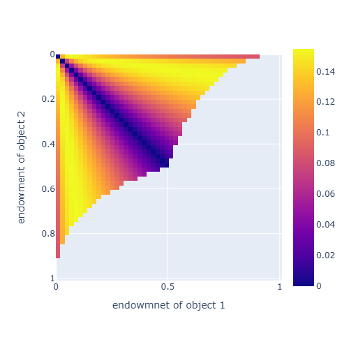
Figure 5: Percentage difference of social welfare between RF and SD $(RS(\mathcal{M}_{RF})-RS(\mathcal{M}_{SD}))/RS(\mathcal{M}_{RF})$.

To evaluate the tradeoff between social welfare and the simplicity of the mechanism, we compare the performance of SD and RF. The allocation probability of RF should satisfy a market-clearing condition. That is, given the allocation probability, agents should optimally choose one option. This determines the demand for each object, and together with the resource constraint, the demand determines the allocation probability. The initial allocation probability should be consistent with the last one. For each pair of endowments $(m_{1},m_{2})$, there exists a unique RF that satisfies the market-clearing condition, and its performance has a closed-form representation when values follow an exponential distribution. The derivation is presented in Appendix A.10.

Figure 5 displays the percentage difference of residual surplus between RF and SD (i.e., $(RS(\mathcal{M}_{RF})-RS(\mathcal{M}_{SD}))/RS(\mathcal{M}_{RF})$) for various endowments, $(m_{1},m_{2})$. For any endowments, RF performs as good as or better than SD. Indeed, when $m_{1}=m_{2}$, RF and SD return an identical allocation and the performance difference is zero. The percentage difference is at most 15%, implying that the gain from using RF is not excessively large.

4 Finite Market

Analyzing finite markets, where a finite number of agents are allocated a finite number of objects, is considerably more challenging than analyzing continuous markets. In this study, instead of characterizing efficient mechanisms, we adopted the deep learning-based approach developed by Dütting et al. (2019), originally for automatically constructing revenue-maximizing auction mechanisms, design mechanisms that maximize residual surplus in finite markets numerically.

4.1 Model

We consider a finite market with a finite set of agents $I$ and a finite set of object types $K$. The endowment of each object type $k$ is $m_{k}$. Slightly abusing notation, $I$ and $K$ also represent the cardinality of those sets. Agents’ utilities are identical to that of the continuous market: When agent $i$ obtains object $k$ with probability $x_{k}^{i}$ for each $k$ while making a payment of $p^{i}$, her payoff is

$$\sum_{k\in K}v_{k}^{i}x_{k}^{i}-p^{i}.$$ (30)

Let $V^{i}\subset\mathbb{R}^{K}$ be the set of all possible valuation vectors for agent $i$, and $\mathbf{v}^{i}$ be its generic element. We define the set of all valuation profiles as $V\coloneqq\bigtimes_{i\in I}V^{i}$, and $\mathbf{v}=(\mathbf{v}^{i})_{i\in I}$ as its generic element. Here, we abandon equal treatment of equals and a direct mechanism $\mathcal{M}$ is comprised of an allocation rule $\mathbf{x}:V\to[0,1]^{I\times K}$ and a payment rule $\mathbf{p}:V\to\mathbb{R}_{+}^{I}$, where $\mathbf{x}^{i}(\mathbf{v})$ and $p^{i}(\mathbf{v})$ are the respective allocation and payment for agent $i$ under valuation profile $\mathbf{v}$. Let $F$ be the probability distribution that valuation profile $\mathbf{v}$ follows.

The residual surplus from a mechanism $\mathcal{M}=(\mathbf{x},\mathbf{p})$ is

$$RS(\mathcal{M})\coloneqq\int_{V}\sum_{i\in I}\left(\sum_{k\in K}v^{i}_{k}x^{i}_{k}(\mathbf{v})-p^{i}(\mathbf{v})\right)dF(\mathbf{v}).$$ (31)

A mechanism $\mathcal{M}$ satisfies the resource constraint if

$$\sum_{i\in I}x^{i}_{k}(\mathbf{v})\leq m_{k}\text{ for all }k\in K,\mathbf{v}\in V.$$ (32)

A mechanism $\mathcal{M}$ is strategy-proof if

$$\sum_{k\in K}v^{i}_{k}x^{i}_{k}(\mathbf{v}^{i},\mathbf{v}^{-i})-p^{i}(\mathbf{v}^{i},\mathbf{v}^{-i})\geq\sum_{k\in K}v^{i}_{k}x^{i}_{k}(\hat{\mathbf{v}}^{i},\mathbf{v}^{-i})-p(\hat{\mathbf{v}}^{i},\mathbf{v}^{-i})\text{ for all }i\in I,\mathbf{v}^{i},\hat{\mathbf{v}}^{i}\in V^{i},\mathbf{v}^{-i}\in V^{-i}.$$ (33)

A mechanism $\mathcal{M}$ is individually rational if

$$\sum_{k\in K}v^{i}_{k}x^{i}_{k}(\mathbf{v})-p^{i}(\mathbf{v})\geq 0\text{ for all }i\in I,\mathbf{v}\in V.$$ (34)

A mechanism $\mathcal{M}$ satisfies the unit demand condition if

$$\sum_{k\in K}x^{i}_{k}(\mathbf{v})\leq 1\text{ for all }i\in I,\mathbf{v}\in V.$$ (35)

A mechanism $\mathcal{M}$ is efficient if it maximizes the residual surplus (31) subject to (32), (33), (34), and (35).

4.2 Numerical Analysis

4.2.1 Methodology

In order to numerically derive an efficient mechanism for finite markets, we adopt RegretNet, a deep learning-based method for designing revenue-maximizing auction mechanisms proposed by Dütting et al. (2019). In RegretNet, a mechanism, which is a function that takes a valuation profile as input and returns an allocation and a payment profile, is represented by a neural network, which can approximate a wide range of functions using a relatively small number of parameters. The loss function used for learning consists of two terms: the negated empirical expected revenue of the seller and a penalty term for violating strategy-proofness, called regret. We use the augmented Lagrange method to find a mechanism (i.e., the network’s parameter) minimizing such loss. In this manner, RegretNet maximizes revenue while minimizing violations of strategy-proofness.

Residual-surplus maximization and revenue maximization have different objective functions but share the same constraints. Therefore, we can derive an efficient money-burning mechanism by simply changing the objective function without making other modifications.

4.2.2 I.I.D. Case

We examine the extent to which the continuous-market model well approximates a finite market. We first consider a market with $4m$ agents and two object types ($K=2$) each with $m\in\mathbb{Z}_{+}$ capacities. Each agent $i$’s value for object $k$, $v_{k}^{i}$ follows Weibull, i.i.d.

For $m=1,5,10$, we generate one million samples and compare the ratio of social welfare achieved by SD and VCG, i.e., $RS(\mathcal{M}_{SD})/RS(\mathcal{M}_{VCG})$. We also plot (i) the ratio in a continuous market with a unit mass of agents and two objects with $m_{k}=0.25$ unit of endowments (i.e., $\bar{m}=0.5$), which corresponds to a finite market in the limit of $m\to\infty$, and (ii) the ratio in a finite market with two agents and one object, which corresponds to the single-good case.

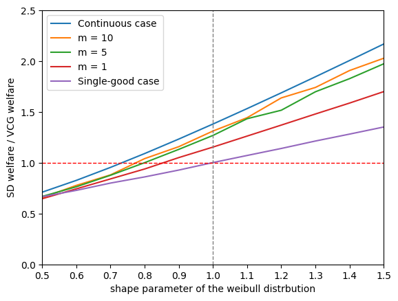
Figure 6: The ratio of the residual surplus achieved by SD and VCG, $(RS(\mathcal{M}_{SD})/RS(\mathcal{M}_{VCG}))$.

Figure 6 shows the results. As characterized by Hartline and Roughgarden (2008), SD outperforms VCG if and only if $\alpha>1$, for the single-good case. Consistent with our theoretical analysis, in the continuous case, SD achieves larger social welfare than VCG as long as the shape parameter is larger than roughly $0.7$, given $K=2$. We observe a similar pattern for finite markets: Even with $m=1$, the threshold at which SD starts to outperform VCG is strictly smaller than $1.0$, and as $m$ increases, the market becomes closer to the continuous case.

Next, we use RegretNet to derive an efficient mechanism for small finite markets. We consider the case of two agents and two objects, where each agent’s value $v_{k}^{i}$ follows (i) Weibull with shape parameter 0.8, and (ii) Weibull with shape parameter 0.7.

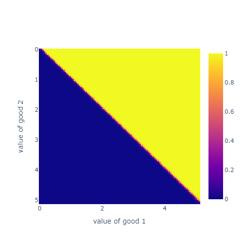
(a) Case (i): $x_{1}^{1}(v_{1}^{1},v_{1}^{2},2,1)$

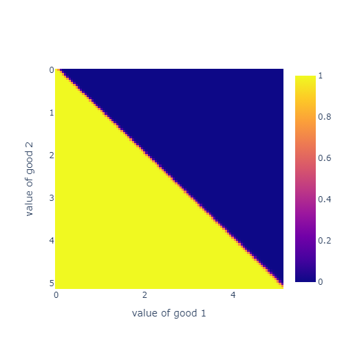
(b) Case (i): $x_{2}^{1}(v_{1}^{1},v_{1}^{2},2,1)$

(c) Case (i): $p^{1}(v_{1}^{1},v_{1}^{2},2,1)$

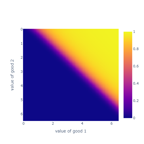
(d) Case (ii): $x_{1}^{1}(v_{1}^{1},v_{1}^{2},2,1)$

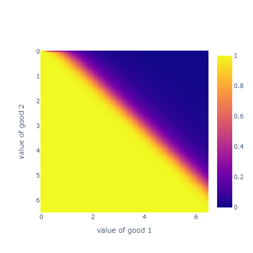
(e) Case (ii): $x_{2}^{1}(v_{1}^{1},v_{1}^{2},2,1)$

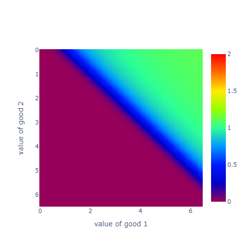
(f) Case (ii): $p^{1}(v_{1}^{1},v_{1}^{2},2,1)$

Figure 7: Allocation and payment for agent 1 from an efficient mechanism learned by RegretNet. Agent 2’s value is fixed to $(v^{2}_{1},v^{2}_{2})=(2,1)$.

Figure 7 shows the approximately efficient mechanisms learned by RegretNet. The horizontal and vertical axis represents $v_{1}^{1}$ and $v_{2}^{1}$, agent $1$’s value for objects $1$ and $2$. Agent $1$’s allocation probability and the amount of agent $1$’s payment are represented by color. While RegretNet returns the full shape of the mechanism, for the illustration’s sake, we fix agent $2$’s valuation to $(v_{1}^{2},v_{2}^{2})=(2,1)$ to draw these figures.

Panels (a), (b), and (c) show the result for case (i). The learned mechanism allocates agent $1$ their favorite object, without payment and regardless of agent $2$’s value, implying that the mechanism is SD that prioritizes agent $1$ over agent $2$. Accordingly, under this setting, despite the marginal value distribution having a DHR, RegretNet still returns SD as an efficient mechanism.

Panels (d), (e), and (f) show the result for case (ii). The value distribution has a thicker tail than case (i), and the learned mechanism allocates the contested object with a price of the other agent’s value—since agent $2$ prefers object $1$ over object $2$ by $v_{1}^{2}-v_{2}^{2}=2-1=1$, agent $1$ obtains object $1$ only if her excess value $v_{1}^{1}-v_{2}^{1}$ is larger than $1$, and agent $1$ has to pay the price of $1$ in such cases. This is how VCG allocates objects.

These results suggest that the trends observed through the analysis of continuous markets are useful even in finite markets, where deriving an efficient mechanism is highly challenging. Specifically, the more strongly the marginal value distribution exhibits DHR, the more likely the efficient mechanism will be VCG. However, in multi-object allocations, even if the marginal value distribution has a DHR, SD can still be (at least approximately) an efficient mechanism.

4.2.3 Correlation

Next, we relax the i.i.d. assumption and investigate cases where values are correlated. The correlation between values $v_{k}^{i}$ can be classified into two patterns. The first is the within-agent correlation, the correlation between $v_{k}^{i}$ and $v_{l}^{i}$ for two distinct objects $k\neq l$ (e.g., some agents need any object more strongly than other agents), and the second is the between-agent correlation, the correlation between $v_{k}^{i}$ and $v_{k}^{j}$ for two distinct agents $i\neq j$ (e.g., some objects are more popular than other agents). In this section, we numerically analyze the effects of both types of correlation on efficient mechanisms. Specifically, we consider the following two cases.

In case (iii), we consider the within-agent correlation. The marginal distribution of $v_{k}^{i}$ is fixed to Weibull with shape parameter $0.8$, the same as case (i) in Subsection 4.2.2, where SD was efficient. Values are independent across agents. With probability $1/2$, the values for the two objects are also drawn independently, the same as an i.i.d. environment. With probability $1/2$, each agent $i=1,2$ receives an identical value for both objects: $v_{1}^{i}=v_{2}^{i}$.

The efficient mechanism for case (iii), illustrated in Figure B.11 in Appendix B.3, is VCG. In the case where the marginal value distribution is the same and all values are drawn independently (case (i) in Subsection 4.2.2), SD was efficient, making this result non-trivial. This suggests that within-agent correlation might attenuate the performance improvement of the no-screening mechanism as the variety of goods increases. In particular, when the within-agent correlation is perfect, each agent has the same value for all objects, and thus the problem essentially has homogeneous goods and single-dimensional types. When the within-agent correlation is intermediate (as in case (iii)), the results are also expected to be intermediate between the single-dimensional type (or perfect correlation) and the multi-dimensional i.i.d. types.

In case (iv), we consider the between-agent correlation. The marginal distribution of $v_{k}^{i}$ is fixed to Weibull with shape parameter $0.7$, the same as case (ii) in Subsection 4.2.2, where VCG is efficient. Values are independent across objects. With probability $1/2$, the two agents’ values are also drawn independently, the same as an i.i.d. environment. With probability $1/2$, the values for each object $k=1,2$ are common across agents: $v_{k}^{1}=v_{k}^{2}$.

In contrast to case (iii), the efficient mechanism for case (iv), illustrated in Figure B.11 in Appendix B.3, is SD, whereas VCG was efficient for case (ii), where values follow the same marginal distribution whereas all values were drawn i.i.d. Compared to the i.i.d. case, no-screening mechanisms are even more advantageous with the between-agent correlation. This is because popular goods will yield high value regardless of to whom they are allocated. As the environment approaches a common value scenario, the benefits of screening diminish, and the performance of SD improves. In contrast, adopting a mechanism that involves screening, such as VCG, would lead to intense competition for popular goods. Consequently, the common value would be lost as a result of money burning.

5 Application: Mass Vaccination against Pandemic Diseases

5.1 Lessons from the COVID-19 Pandemic

The global outbreak of COVID-19 had a profound impact on the world economy and social welfare. In response to the severity of the situation, the development and approval of vaccines for COVID-19 progressed at an unprecedented speed. By the end of 2020, several pharmaceutical companies had successfully developed vaccines, which were deployed with great expectations and indeed achieved significant results. The total number of COVID-19 vaccinations reached 9.14 billion by the end of 2021 (Mathieu et al., 2021), making it arguably the largest allocation problem in history.

Before the start of distribution, clinical trials had confirmed that vaccines were effective in preventing severe illness and the onset of COVID-19, and they were also expected to prevent infection and transmission. Preventing severe illness helped ensure the health and safety of healthcare workers, reduced the number of patients needing hospitalization, and thus prevented the overburdening of medical resources. If vaccines could prevent infection, it could gradually reduce the number of cases and eventually control the pandemic. Therefore, rapidly distributing vaccines to those who need them is crucial for mitigating the impact of the pandemic.

Vaccine production is sequential and gradual, whereas the number of people wishing to be vaccinated and eligible for vaccination is large from the outset. Consequently, at the initial stages of distribution, vaccines are an extremely scarce resource. Although vaccines themselves are largely homogeneous, the reservation slots, defined by the “when, where, and which vaccine,” are heterogeneous, and people have diverse preferences over slots depending on their residence, workplace, convenient dates and times, etc. Developing an efficient system for handling these reservations falls within the realm of market/mechanism design.

Unfortunately, vaccine development progressed too rapidly, and thus mechanism designers were unable to conduct sufficient analysis and make policy recommendations before distribution began. As a result, the logistics of vaccine distribution in many countries did not fully incorporate insights from mechanism design, leading to various confusions. With the advancement of globalization, the possibility of future pandemics from infections other than COVID-19 has been highlighted. On the other hand, improvements in vaccine development technology suggest that effective vaccines can be quickly developed for future pandemics. Researching optimal mass vaccination logistics during normal situations is crucial, not only as a reflection on the COVID-19 pandemic but also for preparedness for future pandemics.

5.2 First-Comes, First-Served (FCFS)

During the COVID-19 pandemic, the most widely used reservation system was based on FCFS. An FCFS system continuously displays currently available (remaining slots). Individuals can access the system at any time, choose their preferred slot, and complete their reservation instantly.

The FCFS system is considered a desirable mechanism during normal times when slots are abundant and individuals do not need to rush to secure a slot. FCFS has various practically desirable properties, including the following:

Simplicity

FCFS is easy to implement as a system and straightforward for participants to understand the rules. Furthermore, once a participant accesses the system, they can easily figure out an optimal action to take.

Low Communication Cost

Under FCFS, each participant only needs to communicate their favorite slot among available ones, reducing communication costs substantially. This information is relatively easy to convey orally via phones, making it convenient for individuals with limited digital literacy.

Immediate Confirmation

With FCFS, reservations are confirmed at the moment the action is taken; thus, participants do not need to hold multiple dates tentatively.

Perhaps for these reasons, the FCFS reservation system is commonly used in our daily lives, and thus the same method was adapted for the special circumstance of pandemic vaccine distribution.

However, in situations where demand far exceeds supply, such as the early stages of pandemic vaccine distribution, the drawbacks of FCFS become more pronounced. In FCFS, participants can secure a reservation by acting faster than others. Thus, it is a screening mechanism that incurs effort costs, and our analysis indicates that such mechanisms are inefficient given that many heterogeneous objects (reservation slots) are allocated. Participants expend substantial effort competing for limited slots, and this cost outweighs the benefit of screening.

During the COVID-19 pandemic, participants’ efforts also raised issues not formally modeled in this paper. Under FCFS, the probability of securing a reservation depends on “how quickly one can access the reservation system,” for online reservations, “how quickly one can call the call center” for phone reservations, or “how early one can go to the vaccination site and line up” for physical site reservations. Such efforts resulted in server crashes, overwhelmed call center lines, and long queues around vaccination sites, causing traffic disruptions in the surrounding areas. While our model treats effort as wasteful but harmless like money burning, in reality, the effort often imposes undue stress on systems and authorities, as well as on residents.

FCFS also has issues with fairness. While some argue that the structure of those who access early get the slots is fair, this claim is not entirely valid. The ability to secure slots that access the system immediately after the start of reservations depends on factors such as whether one can enlist help from family members for booking or if one’s home Internet connection is strong enough. There is no justification for why those with ample resources (but who may not necessarily value the vaccine highly) should find it easier to secure slots.

5.3 Unilateral Assignment

Some authorities, disliking the wasted effort associated with FCFS, employed unilateral assignment mechanisms that do not reflect participants’ preferences for the allocation. In this approach, the authority unilaterally assigns dates and locations for vaccination, and participants receive the vaccine according to these assignments. Participants’ preferences are ignored, thus they do not need to make reservations.

This approach retains the simplicity, low communication cost, and immediate confirmation of vaccination appointments, all practical and desirable features akin to FCFS. Since unilateral assignment is a no-screening mechanism, it does not induce unnecessary effort and avoids the disruption caused by FCFS. In Japan, where society was troubled by the chaos of FCFS, unilateral assignment was favorably reported and shared as a success story on the Prime Minister’s Office website.

However, unilateral assignment disregards the information on preference order, which can be utilized without incurring screening costs. Therefore, in our model (which ignores the cost of making reservations itself), unilateral assignment is dominated by SD and is never output as an optimal mechanism. Obviously, it also lacks performance guarantees in the worst-case scenario. Additionally, it is important to note that the successful examples reported in Japan mainly involved vaccinations for the elderly, who had fewer unacceptable dates and times.

5.4 Direct-Mechanism Implementation of SD

In Kakogawa City, Japan, a mechanism similar to a direct-mechanism implementation of SD, was employed for distributing vaccines to residents aged 65 and over (Tada, 2021). Initially, the city used FCFS, but like other municipalities, this led to an overwhelming number of server accesses and numerous complaints to the call center. Consequently, Kakogawa City switched to a lottery system that treated all applications equally if submitted by the deadline.

In this implementation, batches of reservation slots were created at regular intervals and allocated simultaneously. Participants could indicate whether they found available dates, times (morning or afternoon), and five mass vaccination sites in the city acceptable. The priority within the participants, all of whom were 65 years or older, was determined randomly. Reservation slots were then allocated sequentially to those who had declared them acceptable based on their randomly assigned priority.

The mechanism in Kakogawa City was also reported favorably and featured on the Prime Minister’s Office website as a successful case. However, for vaccinations of residents under 65, the city reverted to FCFS, citing the increased complexity of preferences regarding dates and locations. While Kakogawa City attempted to reduce communication costs by asking participants to declare whether slots were acceptable rather than ranking them in order of preference, this adjustment reduces the cardinality of all possible reports only from $K!$ to $2^{K}$, which was not entirely sufficient. In addition, the implementation in Kakogawa City required participants to keep all potential dates open until the lottery draw, which does not provide immediate confirmation of appointments.

5.5 Register-Invite-Book System (RIB)

Finally, we introduce the register-invite-book system (RIB), a mechanism that is the most suitable for handling pandemic vaccine appointments in our opinion. This mechanism is similar to SD in sequential form and was effectively used for COVID-19 vaccine distribution in places including British Columbia, Canada, and Singapore.

As the name suggests, RIB first requires participants to complete registration. By registering, participants provide contact information such as an email address and input information relevant to their priority (e.g., age, occupation, underlying health condition). At this stage, no information about participants’ preferences over slots is entered. The system sorts the registered participants using methods other than FCFS, such as age or a lottery. The system sequentially sends an invitation to the next participant in line, while controlling the timing taking into account the current availability of reservation slots (i.e., sends invitations more rapidly if many slots are remaining). Upon receiving an invitation, participants access the system and select their preferred slot from available options to complete their booking on an FCFS basis.

The final stage of RIB retains the desirable practical properties of FCFS: simplicity, low communication cost, and immediate confirmation. However, because invitations are sent gradually, the incentive for participants to exert effort to secure a slot is low, as only a few can be overtaken by accessing the system immediately after being invited. Therefore, RIB is approximately a no-screening mechanism and equivalent to SD implemented in sequential form, sorting agents by an exogenous priority order and allowing them to choose their most preferred remaining slot in turn. RIB thus combines the practical advantages of FCFS with the theoretically desirable properties of SD, particularly the tendency to be an efficient mechanism when many heterogeneous objects are allocated, as discussed in this paper.

In the application of vaccine distribution, RIB has other noteworthy advantages. First, it is easy to prioritize specific groups of people. Those at higher risk, those prioritized for reasons of fairness, and those prioritized to prevent the spread of infection are likely to emerge for many diseases and vaccines, as discussed by Pathak et al. (2022, 2024); Akbarpour et al. (2023). This prioritization can be even more important than willingness to pay based on the effort cost reflecting how strongly someone wants the good. In RIB, policymakers can freely adjust the order in which invitations are sent. Although this paper’s model assumes that all agents are ex ante symmetric, the no-screening mechanism’s superiority should be maintained regardless of how priority is set.

Second, RIB minimizes communication costs in the case of gradually supplied goods. When goods are gradually supplied other mechanisms typically suffer from increased communication costs. For instance, FCFS used in New York City released slots for several days ahead every midnight; thus, participants had to repeatedly access the system every night until they successfully made a reservation, which imposed unnecessary effort on participants and increased server load. Implementing SD as a direct mechanism would require creating a new lottery notification each time vaccines are supplied to the city and having participants submit their preferences for new dates, which incurs significant unmodeled costs. In contrast, with RIB, participants only need to access the system once to register and do not need to access it again until they receive an invitation. This property greatly reduces communication costs even compared with FCFS.

Finally, RIB allows participants to predict when they might secure a reservation slot more easily. Vaccines are supplied sequentially, and all participants will eventually receive a vaccination. However, under FCFS, the competition for slots occurs each time new slots are released, thereby participants cannot predict their chances of securing a slot based on past attempts. In other words, there is no assurance that having participated in many previous rounds of competition will increase their likelihood of securing a slot in the future. This uncertainty persists until a reservation is secured, requiring participants to keep potential dates open and causing mental stress. In contrast, with RIB, the system can continuously disclose how many people have higher priority, allowing participants to estimate when their turn might come. Although the exact timing can be difficult to predict due to potential new registrations and uncertainties in vaccine supply, RIB provides a much clearer and more predictable framework compared to FCFS.

In addition to the various advantages of the sequential form of SD discussed in Section 2, RIB further enhances these benefits in the context of pandemic vaccine distribution. This paper also demonstrates that even when framing the vaccine distribution problem purely as efficient screening through money burning, no-screening mechanisms like SD perform well in a wide range of situations, as long as multiple goods are allocated. Therefore, at present, RIB can be considered a state-of-the-art mechanism for the distribution of pandemic vaccines.

6 Concluding Remarks

We studied the efficient money-burning mechanism for allocating multiple heterogeneous goods, where agents can take costly actions to signal the magnitude of their values. We found that as the variety of goods increases, the performance of no-screening mechanisms like SD improves.

We first explored this trend by analyzing a stylized environment with continuously many agents and objects, assuming the values for all object types are drawn i.i.d., and the capacity of each object type is uniform. Agents tend to acquire the goods they prefer more. As the variety of goods increases, the distribution of the value for the “more preferred goods,” which is the largest order statistic in the i.i.d. environment, increasingly favors no-screening mechanisms. We further applied extreme value theory—a long-established but previously unused technology in mechanism design—and proved that in the limit of the large variety, the efficient mechanism involves little to no screening.

Second, we applied the automated mechanism design method established by Dütting et al. (2019) for revenue maximization to numerically explore efficient money-burning mechanisms. The results showed that several strong assumptions imposed on the stylized environment—such as the continuously many agents and objects, the very large variety $K$, the i.i.d. draw of marginal values $v_{k}^{i}$ for each agent $i$ and object $k$, and the uniform capacity for each object type $k$—are not essential to the trend that no-screening mechanisms tend to be efficient in multi-object allocations. This finding implies that no-screening mechanisms can perform well in practical settings. Considering the various excellent properties of SD discussed in previous studies, this result suggests that SD is a promising option.

Third, as an application, we discussed the implication of our findings for pandemic vaccine distribution. Since reservation slots specifying when and where the vaccine is administered are heterogeneous goods, managing vaccine appointments is a problem of allocating a large number of heterogeneous goods. This paper demonstrates that using mechanisms like FCFS, where effort costs increase the probability of obtaining desired goods, is inefficient for this problem. While there are various mechanisms and implementations within the class of no-screening mechanisms, RIB stands out. RIB, which has theoretical properties close to those of SD in sequential form and user experience akin to FCFS, is likely the state-of-the-art method for distribution at this time.

Finally, we make two concluding remarks for future research and policy design. First, while this paper primarily discusses vaccine distribution as its main application, the issue of policymakers allocating goods without monetary transfers is commonplace. This paper offers policy implications for all such problems. In particular, the justification for imposing burdensome administrative procedures to ensure that only those who truly need goods and services receive them may be valid in far fewer situations than previously thought. Second, although the immediate problem of COVID-19 vaccine distribution has subsided at the time of writing, this does not imply that pandemic vaccine distribution is no longer a crucial issue. We should have learned from COVID-19 that once a pandemic begins, most societal resources are directed toward managing the crisis, leaving little time to research and develop new mechanisms. Now that we have the time for thorough research and development, we must work on implementing mechanisms like RIB or develop more effective mechanisms that may exist.

Appendix

Appendix A Proofs

A.1 Proof of Theorem 1

Proof.

We show the contraposition. Suppose that there exist $V^{*}\subset V$ with $F(V^{*})>0$ and $k^{-}\in K$ such that $k^{-}\notin\operatorname*{arg\,max}_{l\in K}v_{l}$ whereas $x_{k^{-}}(\mathbf{v})>0$. Take $k^{+}\in\operatorname*{arg\,max}_{l\in K}v_{l}$ arbitrarily. We define a mapping $T:V\to V$ by

$$Tv_{k^{+}}=v_{k^{-}},Tv_{k^{-}}=v_{k^{+}},Tv_{k}=v_{k}\text{ for all }k\in K\setminus\{k^{+},k^{-}\}.$$ (36)

By object-symmetry, we have $x_{k^{+}}(\mathbf{v})=x_{k^{-}}(T\mathbf{v})$, $x_{k^{-}}(\mathbf{v})=x_{k^{+}}(T\mathbf{v})$, and $x_{k}(\mathbf{v})=x_{k}(T\mathbf{v})$ for all $k\in K\setminus\{k^{+},k^{-}\}$. We define an alternative allocation rule $\mathbf{x}^{\prime}$ by

$$x^{\prime}_{k^{+}}(\mathbf{v}) =x_{k^{+}}(\mathbf{v})+x_{k^{-}}(\mathbf{v})\text{ for all }\mathbf{v}\in V^{*},$$ (37)

$$x^{\prime}_{k^{-}}(\mathbf{v}) =0\text{ for all }\mathbf{v}\in V^{*},$$ (38)

$$x^{\prime}_{k^{+}}(\mathbf{v}) =0\text{ for all }\mathbf{v}\in TV^{*},$$ (39)

$$x^{\prime}_{k^{-}}(\mathbf{v}) =x_{k^{+}}(\mathbf{v})+x_{k^{-}}(\mathbf{v})\text{ for all }\mathbf{v}\in TV^{*},$$ (40)

$$x^{\prime}_{k}(\mathbf{v}) =x_{k}(\mathbf{v})\text{ otherwise.}$$ (41)

By construction, $\sum_{k\in K}x^{\prime}_{k}(\mathbf{v})=\sum_{k\in K}x_{k}(\mathbf{v})\leq 1$, implying that $\mathbf{x}^{\prime}$ satisfies the unit demand condition. Furthermore, since we have $F(\mathbf{v})=F(T\mathbf{v})$ in an i.i.d. environment, the resource constraint is also satisfied. Furthermore, all agents with valuation $\mathbf{v}\in V^{*}\cup TV^{*}$ prefers $\mathbf{x}^{\prime}$ over $\mathbf{x}$, whereas $F(V^{*})>0$ by assumption. Accordingly, $\mathbf{x}$ is not ex post efficient. ∎

A.2 Proof of Theorem 3

Proof.

Recall that

$$r(v;G_{K})=\frac{g_{K}(v)}{1-G_{K}(v)}=\frac{Kg(v)(G(v))^{K-1}}{1-(G(v))^{K}}.$$ (42)

By direct calculation, we can show that

$$r^{\prime}(v;G_{K})=\frac{K(G(v))^{K-2}}{(1-(G(v))^{K})^{2}}\left(K(g(v))^{2}-((g(v))^{2}-g^{\prime}(v)G(v))(1-(G(v))^{K})\right).$$ (43)

Thus, $r^{\prime}(v;G_{K}))\geq 0$ if and only if

$$K(g(v))^{2}\geq((g(v))^{2}-g^{\prime}(v)G(v))(1-(G(v))^{K}).$$ (44)

We show that, for any fixed $v$, if (44) holds with $K$, then (44) also holds with $K+1$. This claim is trivial if $g^{\prime}(v)\geq 0$. In the following, we consider the case of $g^{\prime}(v)<0$.

Suppose that (44) holds with $K$. Then, we have

$$K(g(v))^{2}\geq((g(v))^{2}-g^{\prime}(v)G(v))(1-(G(v))^{K}).$$ (45)

and thus

$$(K+1)(g(v))^{2}\geq((g(v))^{2}-g^{\prime}(v)G(v))\frac{K+1}{K}(1-(G(v))^{K}).$$ (46)

Therefore, it suffices to show that

$$\frac{K+1}{K}(1-x^{K})\geq 1-x^{K+1}$$ (47)

for all $x\in[0,1]$, or equivalently,

$$(K+1)(1-x^{K})-K(1-x^{K+1})\geq 0.$$ (48)

It follows from $1-x^{K}=(1-x)(x^{K-1}+x^{K-2}+\dots+x+1)$ that (48) holds if

$$(K+1)(x^{K-1}+x^{K-2}+\dots+x+1)-K(x^{K}+x^{K-1}+\dots+x+1)\geq 0,$$ (49)

or equivalently,

$$x^{K-1}+\dots+x+1\geq Kx^{K}.$$ (50)

Indeed, (50) holds for all $x\in[0,1]$ because $x^{k}\geq x^{K}$ holds for all $k=0,1,\dots,n-1$, as desired.

We show that for all $v\in[0,\bar{v}]$, there exists $K_{0}$ such that for all $K>K_{0}$, $r^{\prime}(v;G_{K})>0$. The right-hand side of (44) is bounded above by $((g(v))^{2}-g^{\prime}(v)G(v))$. Since we assume that $f$ has full support, i.e., $g(v)>0$ for all $v\in[0,\bar{v}]$, there exists $K_{0}$ such that

$$K_{0}(g(v))^{2}>(g(v))^{2}-g^{\prime}(v)G(v).$$ (51)

Clearly, for all $K>K_{0}$, we have (44), implying that $r^{\prime}(v;K)>0$. ∎

A.3 Proof of Theorem 4

Proof.

Take $\epsilon>0$ and $\delta>0$ arbitrarily. Let $\bar{\delta}=\min\{\delta,(1-\bar{m})/2\}$. Since $\bar{v}=\sup\text{support}(G)<+\infty$, we have $G(\bar{v}-\epsilon)<1$. Let $K_{0}$ be the smallest integer $K$ satisfying $G_{K}(\bar{v}-\epsilon)\coloneqq(G(\bar{v}-\epsilon))^{K}<\bar{\delta}$, i.e., $K_{0}=\lfloor\log\bar{\delta}/\log G(\bar{v}-\epsilon)\rfloor$. By construction of $K_{0}$, for any $K>K_{0}$, we have $G_{K}(\bar{v}-\epsilon)<\bar{\delta}$, or equivalently, $\Pr(v\in(\bar{v}-\epsilon,\bar{v}])>1-\bar{\delta}$.

Given such $K_{0}$, for any $K>K_{0}$,

$$RS(\mathcal{M}_{SD}) =\bar{m}\int_{0}^{\bar{v}}vdG_{K}(v)$$ (52)

$$>\bar{m}\int_{\bar{v}-\epsilon}^{\bar{v}}(\bar{v}-\epsilon)dG_{K}(v)$$ (53)

$$=\bar{m}\Pr(v\in(\bar{v}-\epsilon,\bar{v}])(\bar{v}-\epsilon)$$ (54)

$$>\bar{m}(1-\bar{\delta})(\bar{v}-\epsilon)$$ (55)

$$\geq\bar{m}(1-\delta)(\bar{v}-\epsilon).$$ (56)

Next, we evaluate $RS(\mathcal{M}_{VCG})$ with the same $K_{0}$. For any $K>K_{0}$, we have $G_{K}(\bar{v}-\epsilon)<\bar{\delta}<1-\bar{m}$. Accordingly, we have $q\coloneqq G_{K}^{-1}(1-\bar{m})>\bar{v}-\epsilon$. Accordingly,

$$RS(\mathcal{M}_{VCG}) =\int_{q}^{\bar{v}}\left(v-q\right)dG_{K}(v)$$ (57)

$$<\int_{\bar{v}-\epsilon}^{\bar{v}}\left(\bar{v}-(\bar{v}-\epsilon)\right)dG_{K}(v)$$ (58)

$$=\epsilon(1-G_{K}(\bar{v}-\epsilon))$$ (59)

$$<\bar{m}\epsilon.$$ (60)

∎

A.4 Proof of Lemma 1

Proof.

Recall that $\vartheta^{\prime}(w;\hat{G}_{K})\coloneqq(1-\hat{G}_{K}(w))/\hat{g}_{K}(w)$.

$$\vartheta^{\prime}(w;\hat{G}_{K})\coloneqq\left(\frac{1-\hat{G}_{K}(w)}{\hat{g}_{K}(w)}\right)^{\prime}=\frac{-(\hat{g}_{K}(w))^{2}-\hat{g}^{\prime}_{K}(w)(1-\hat{G}_{K}(w))}{(\hat{g}_{K}(w))^{2}}.$$ (61)

Since $G$ has full support and twice differentiable, there exists $\underline{g}$ such that $\hat{g}_{K}(w)>\underline{g}$ for all $w\in[\underline{c},\bar{c}]$. Furthermore, $\hat{G}_{K},\hat{g}_{K},\hat{g}^{\prime}_{K}$ converges uniformly to $\Lambda,\lambda,\lambda^{\prime}$ in $[\underline{c},\bar{c}]$. Accordingly, for all $w\in[\underline{c},\bar{c}]$,

$$\vartheta^{\prime}(w;\hat{G})\to\frac{-(\lambda(w))^{2}-\lambda^{\prime}(w)(1-\Lambda(w))}{(\lambda(w))^{2}}=\vartheta^{\prime}(w;\Lambda)<0,$$ (62)

where the convergence is uniform in $[\underline{c},\bar{c}]$. Hence, there exists $K_{0}$ such that for all $K>K_{0}$, we have $\vartheta^{\prime}(w;\hat{G}_{K})<0$ for $w\in[\underline{c},\bar{c}]$.

∎

A.5 Proof of Lemma 2

This lemma is a basic step in deriving revenue-maximizing mechanisms and has been well-known. We include it here for completeness. The proof follows the approach outlined in Fu (2017).

Proof.

Since $x$ is an allocation rule of a strategy-proof mechanism, $x$ is monotonic; thus, $\tilde{x}$ is also monotonic.

Next, we show that $\tilde{x}$ satisfies the resource constraint.

$$\int_{0}^{\bar{v}}\tilde{x}(v)g_{K}(v)dv$$ (63)

$$=\int_{a}^{b}\tilde{x}(v)g_{K}(v)dv+\int_{v\notin[a,b]}x(v)g_{K}(v)dv$$ (64)

$$=(G_{K}(a)-G_{K}(b))\dfrac{\int_{a}^{b}x(w)g_{K}(w)dw}{G_{K}(a)-G_{K}(b)}+\int_{v\notin[a,b]}x(v)g_{K}(v)dv$$ (65)

$$=\int_{0}^{\bar{v}}x(v)g_{K}(v)dv.$$ (66)

Since $x$ satisfies the resource constraint, $\tilde{x}$ also satisfies it.

For $v\notin[a,b]$, $x$ and $\tilde{x}$ are identical and hence generate the same residual surplus. On $[a,b]$, let $G_{K}(\cdot|v\in[a,b])$ denote the conditional distribution of $v$ given $v\in[a,b]$, which has density $g_{K}/(G_{K}(b)-G_{K}(a))$. Then,

$$\int_{a}^{b}\tilde{x}(v)\vartheta(v)g_{K}(b)dv$$ (67)

$$=\dfrac{\int_{a}^{b}x(w)g_{K}(w)dw}{G_{K}(a)-G_{K}(b)}\int_{a}^{b}\vartheta(v)g_{K}(v)dv$$ (68)

$$=\mathbb{E}_{v\sim G_{K}(\cdot|v\in[a,b])}[x(v)]\mathbb{E}_{v\sim G_{K}(\cdot|v\in[a,b])}[\vartheta(v)](G_{K}(b)-G_{K}(a))$$ (69)

$$\geq\mathbb{E}_{v\sim G_{K}(\cdot|v\in[a,b])}[x(v)\vartheta(v)](G_{K}(b)-G_{K}(a))$$ (70)

$$=\int_{a}^{b}x(v)\vartheta(v)g_{K}(b)dv.$$ (71)

The inequality is an application of Harris inequality, which states that for any nondecreasing function $f$ and nonincreasing function $g$ on $\mathbb{R}$ and any probability measure on $\mathbb{R}$, we have $\mathbb{E}[fg]\leq\mathbb{E}[f]\mathbb{E}[g]$.

∎

A.6 Proof of Theorem 5

Proof.

Given for any $\epsilon>0$, take $\bar{c}$ and $\underline{c}$ to satisfy $1-\epsilon/2<(\Lambda(\bar{c})-\Lambda(\underline{c}))$. Then, since $\hat{G}_{K}(w)\to\Lambda(w)$ as $K\to\infty$, there exists $K_{0}$ such that for all $K>K_{0}$, we have $1-\epsilon<\hat{G}_{K}(\bar{c})-\hat{G}_{K}(\underline{c})$. Lemmas 1 and 2 imply that there also exists $K_{0}$ such that for all $K>K_{0}$, for all $w\in[\underline{c},\bar{c}]$, $\hat{x}(w)=\bar{x}$. Let $K_{0}$ be the larger one of these two. Then, clearly we have $\Pr(\hat{x}(w)=\bar{x})>1-\epsilon$. Furthermore, the resource constraint implies that

$$\bar{m}=\int_{0}^{\infty}\hat{x}(w)\hat{G}_{K}(w)dw\geq\int_{\underline{c}}^{\bar{c}}\hat{x}(w)\hat{G}_{K}(w)dw>\bar{x}(1-\epsilon),$$ (72)

or equivalently, $\bar{x}<\bar{m}/(1-\epsilon)$. The resource constraint also implies

$$\bar{m}=\int_{0}^{\infty}\hat{x}(w)\hat{G}_{K}(w)dw\leq\int_{\underline{c}}^{\bar{c}}\hat{x}(w)\hat{G}_{K}(w)dw+\int_{w\notin[\underline{c},\bar{c}]}1\cdot\hat{G}_{K}(w)dw=(1-p)\bar{x}+p,$$ (73)

where $p=\Pr(w\notin[\underline{c},\bar{c}])<\epsilon$. The above inequality can be rewritten as $\bar{x}\geq(\bar{m}-p)/(1-p)$. The right-hand side is larger than $(\bar{m}-\epsilon)/(1-\epsilon)$ because it is decreasing in $p$ and $p>\epsilon$. Accordingly, $\bar{x}>(\bar{m}-\epsilon)/(1-\epsilon)$.

∎

A.7 Proof of Lemma 3

Proof.

We apply the construction of the ironed virtual value established in Section 6 of Myerson (1981) to an IDHR distribution function $G_{K}$. As summarized by Hartline and Roughgarden (2008), the ironed virtual value $\bar{\theta}$ is constructed as follows:

1. For $q\in[0,1]$, define $h(q)=\vartheta(G_{K}^{-1}(q);G_{K})$.

2. Define $H(q)=\int_{0}^{q}h(r)dr$.

3. Define $I$ as the convex hull of $H$, the largest convex function bounded above by $H$ for all $q\in[0,1]$.

4. Define $i(q)$ as the derivative of $I(q)$, where defined, and extend to all of $[0,1]$ by right continuity.

5. $\bar{\vartheta}(v;G_{K})=i(G_{K}(v))$.

Since $G_{K}$ has an IDHR, $H$ is concave for $[0,G_{K}{v^{*}})$ and convex for $(G_{K}(v^{*}),+\infty)$. Accordingly, there exists a unique line passing through the origin and being tangent to $H$. Let the $q$-coordinate of the point of tangency be $q^{**}$. Then, the convex hull $I$ of $H$ is given by

$$I(q)=\begin{cases}\dfrac{H(q^{**})}{q^{**}}\cdot q&\text{ for }q<q^{**}\\ G(q)&\text{ for }q\geq q^{**},\end{cases}$$ (74)

implying that the ironed virtual value is given by (25), where $v^{**}=G_{K}^{-1}(v^{**})$.

Furthermore, since $q^{**}$ is defined as the point of tangency, it solves $H(q)/q=h(q)$, or equivalently,

$$\frac{\int_{0}^{q}\vartheta(G_{K}^{-1}(r))dr}{q}=\vartheta(G_{K}^{-1}(q)).$$ (75)

Finally, we obtain (26) by replacing $q$ with $G_{K}(v)$ and applying the substitution $r=G_{K}(v)$ to the integral in the left-hand side.

∎

A.8 Proof of Theorem 6

Proof.

By Theorem 3, for sufficiently large $K$, there exists $\tilde{c}>0$ such that $\hat{G}_{K}$ has an IHR in $[0,\tilde{c})$. Take $\underline{c}<\tilde{c}$ and $\bar{c}>w^{**}$. It follows from $G\in\textbf{VMC}(1/\alpha)$ and Proposition 3 that $\hat{G}_{K},\hat{g}_{K},\hat{g}^{\prime}_{K}$ converges uniformly to $\hat{G}_{\alpha},\hat{g}_{\alpha},\hat{g}^{\prime}_{\alpha}$ in $[\underline{c},\bar{c}]$. Accordingly, for any $\delta^{\prime}>0$, for sufficiently large $K$, $\hat{G}_{K}$ has an IHR for $[0,w^{*}-\delta^{\prime})$.

Since $\vartheta(\cdot;\hat{G}_{K})$ is decreasing for $[0,w^{*}-\delta^{\prime})$, there exists $w^{\dagger}>w^{*}-\delta^{\prime}$ such that $\hat{x}(w)=\bar{x}$ for $w\in[0,w^{\dagger})$. For a reduced distribution $\hat{G}$, define $\Theta(w;\hat{G})$ by

$$\Theta(w;\hat{G})\coloneqq\dfrac{\displaystyle\int_{0}^{w}\vartheta(w^{\prime};\hat{G})\hat{g}(w^{\prime})dw^{\prime}}{\hat{G}(w)-\vartheta(w;\hat{G})}.$$ (76)

For the same reasons used in the proof of Lemma 3, $w^{\dagger}$ must solve $\Theta(w;\hat{G}_{K})=0$, and $w^{**}$ must solve $\Theta(w;\Phi_{\alpha})=0$. Since $\Phi_{\alpha}$ has an IDHR, $\Theta(\cdot;\Phi_{\alpha})$ is increasing in the neighborhood of $w^{**}$. Furthermore, for any $\delta^{\prime\prime}>0$, by taking sufficiently large $K$, we can make

$$|\Theta(w;\hat{G}_{K})-\Theta(w;\Phi_{\alpha})|<\delta^{\prime\prime}.$$ (77)

Accordingly, for any $\epsilon>0$, for sufficiently large $K$, $w^{\dagger}\in(w^{**}-\epsilon,w^{**}+\epsilon)$. Together with the fact that $\hat{G}_{K}(w)\to\Phi_{\alpha}(w)$ uniformly in $[\underline{c},\bar{c}]$, we have the desired conclusion.

∎

A.9 Efficient Mechanism for a Fréchet Case

We transform (26) to derive (29) as follows.

$$0 =\dfrac{\int_{0}^{v}\vartheta(w;\Phi_{\alpha})\phi_{\alpha}(w)dw}{\Phi_{\alpha}(v)}-\vartheta(v;\Phi_{\alpha}),$$ (78)

$$0 =\dfrac{\int_{0}^{v}(1-\Phi_{\alpha}(w))dw}{\Phi_{\alpha}(v)}-\frac{1-\Phi_{\alpha}(v)}{\phi_{\alpha}(v)},$$ (79)

$$0 =\int_{0}^{v}(1-e^{-v^{-\alpha}})dv-\frac{1-e^{-v^{-\alpha}}}{\alpha v^{-\alpha-1}},$$ (80)

$$0 =\left[v-\frac{1}{\alpha}\Gamma\left(-\frac{1}{\alpha},v^{-\alpha}\right)\right]^{v}_{0}-\frac{1-e^{-v^{-\alpha}}}{\alpha v^{-\alpha-1}},$$ (81)

$$0 =v-\frac{1}{\alpha}\Gamma\left(-\frac{1}{\alpha},v^{-\alpha}\right)-\frac{1-e^{-v^{-\alpha}}}{\alpha v^{-\alpha-1}},$$ (82)

$$0 =v-\frac{1}{\alpha}(-\alpha)\left[\Gamma\left(1-\frac{1}{\alpha},v^{-\alpha}\right)-ve^{-v^{-\alpha}}\right]-\frac{1-e^{-v^{-\alpha}}}{\alpha v^{-\alpha-1}},$$ (83)

$$0 =(1-e^{-v^{-\alpha}})v+\Gamma\left(\frac{\alpha-1}{\alpha},v^{-\alpha}\right)-\frac{1}{\alpha}v^{\alpha+1}(1-e^{-v^{-\alpha}}).$$ (84)

A.10 Random Favorite (RF) Mechanism

We characterize the RF mechanism for the following setting:

• A continuous i.i.d. market.

• Two object types: $K=2$.

• The marginal value distribution is standard exponential: $G(v)=1-e^{-v}$.

• The capacities of objects $1$ and $2$ are given by $(m_{1},m_{2})$, where $m_{1}\geq m_{2}>0$ and $m_{1}+m_{2}\leq 1$.

RF offers two options: without making any payments, (i) obtain object $1$ with probability $a\in(0,1]$ and obtain object $2$ with a zero probability, or (ii) obtain object $2$ with probability $b\in(0,1]$ and obtain object $1$ with a zero probability. An agent claims object $1$ if $av_{1}\geq bv_{2}$, or equivalently, $av_{1}/b\geq v_{2}$ and claims object $2$ otherwise.

Conditional on $v_{1}$, the probability that an agent claims object $2$ is $1-G(av_{1}/b)=e^{-av_{1}/b}$. Thus, the total mass of agents who claim object $2$ is

$$\int_{0}^{\infty}e^{-\frac{a}{b}v_{1}}e^{-v_{1}}dv_{1}=\frac{b}{a+b}.$$ (85)

Accordingly, given $(a,b)$, the demand for object $1$ is $a^{2}/(a+b)$ and the demand for object $2$ is $b^{2}/(a+b)$. The market clearing condition requires that $a^{2}/(a+b)=m_{1}$ and $b^{2}/(a+b)=m_{2}$. Solving these equations, we obtain $a=m_{1}+\sqrt{m_{1}m_{2}}$ and $b=m_{2}+\sqrt{m_{1}m_{2}}$ as a unique $(a,b)$ satisfying the agent’s optimality condition and the market clearing condition.

The residual surplus achieved by RF is

$$RS(\mathcal{M}_{RF})$$ (86)

$$=a\int_{0}^{\infty}v_{1}(1-e^{-\frac{a}{b}v_{1}})e^{-v_{1}}dv_{1}+b\int_{0}^{\infty}v_{2}(1-e^{-\frac{b}{a}v_{2}})e^{-v_{2}}dv_{2}$$ (87)

$$=a\left(1-\frac{b^{2}}{(a+b)^{2}}\right)+b\left(1-\frac{a^{2}}{(a+b)^{2}}\right)$$ (88)

$$=(a+b)-\frac{ab(a+b)}{(a+b)^{2}}$$ (89)

$$=m_{1}+m_{2}+2\sqrt{m_{1}m_{2}}-\sqrt{m_{1}m_{2}}$$ (90)

$$=m_{1}+m_{2}+\sqrt{m_{1}m_{2}}.$$ (91)

Next, we compute the residual surplus achieved by SD. Since $m_{1}\geq m_{2}$ and objects $1$ and $2$ are equally popular, in the beginning, all agents obtain their favorite objects, and object $2$ is exhausted when the first $2m_{2}(<m_{1}+m_{2}<1)$ unit of agents makes a choice. Afterward, all agents obtain object $1$, and when an additional $m_{1}-m_{2}$ unit of agents makes a choice, object $1$ is also exhausted. Accordingly, the residual surplus achieved by SD is

$$RS(\mathcal{M}_{SD})$$ (92)

$$=2m_{2}\int_{0}^{\infty}vg_{2}(v)dv+(m_{1}-m_{2})\int_{0}^{\infty}vg(v)dv$$ (93)

$$=2m_{2}\int_{0}^{\infty}v(2e^{-v}-2^{-2v})dv+(m_{1}-m_{2})\int_{0}^{\infty}ve^{-v}dv$$ (94)

$$=3m_{2}+(m_{1}-m_{2})$$ (95)

$$=m_{1}+2m_{2}.$$ (96)

Since we assume $m_{1}\geq m_{2}$, $RS(\mathcal{M}_{RF})\geq RS(\mathcal{M}_{SD})$ always holds, and the equality holds if and only if $m_{1}=m_{2}$. In Figure 5, we plot

$$\frac{RS(\mathcal{M}_{RF})-RS(\mathcal{M}_{SD})}{RS(\mathcal{M}_{RF})}=\frac{\sqrt{m_{1}m_{2}}-\min\{m_{1},m_{2}\}}{m_{1}+m_{2}+\sqrt{m_{1}m_{2}}}$$ (97)

to illustrate the performance difference between RF and SD.

Appendix B Supplementary Materials

B.1 Supplementary Materials for Section 1

This section details the example of the Weibull distribution with shape parameter $0.9$, which is described as Figure 1 of the introduction.

The Weibull distribution with shape parameter $\alpha>0$ is given by

$$G(v)=1-\exp(-v^{\alpha}),$$ (98)

and its probability density function is

$$g(v)=\alpha v^{\alpha-1}\exp(-v^{\alpha}).$$ (99)

Note that Weibull has an IHR if $\alpha\geq 1$ and a DHR if $\alpha\leq 1$. When $\alpha=1$, it is identical to a standard exponential distribution.

The inverse hazard rate is given by

$$\vartheta(v;G)=\frac{1-G(v)}{g(v)}=\frac{1}{\alpha}v^{1-\alpha}$$ (100)

and thus

$$\vartheta^{\prime}(v;G)=\frac{1-\alpha}{\alpha}v^{-\alpha}\to 0\text{ as }v\to\infty,$$ (101)

implying that the Weibull distribution satisfies the von Mises condition (Definition 5) for all $\alpha>0$, implying that the Weibull distribution belongs to the twice differentiable domain of attraction of Gumbel.

When $G$ is the Weibull distribution with shape parameter $\alpha$, from (16), we have

$$a_{K}=\frac{K}{\alpha}\Gamma\left(\frac{1}{\alpha},\log K\right),\>b_{K}=\left(\log K\right)^{\frac{1}{\alpha}}.$$ (102)

The probability density of the normalized probability density function, which is illustrated as Panel (a) of Figure 1 is given by $\hat{g}_{K}(w)=a_{K}g_{K}(a_{K}w+b_{K})$. The normalized hazard rate is given by

$$r(w;\hat{G}_{K})=\frac{a_{K}g_{K}(a_{K}w+b_{K})}{1-G_{K}(a_{K}w+b_{K})},$$ (103)

and its derivative, illustrated as Panel (b) of Figure 1, is given by

$$r^{\prime}(w;\hat{G}_{K})=\frac{a_{K}^{2}g^{\prime}_{K}(a_{K}w+b_{K})(1-G_{K}(a_{K}w+b_{K}))+a_{K}^{2}g_{K}^{2}(a_{K}w+b_{K})}{(1-G_{K}(a_{K}w+b_{K}))^{2}}.$$ (104)

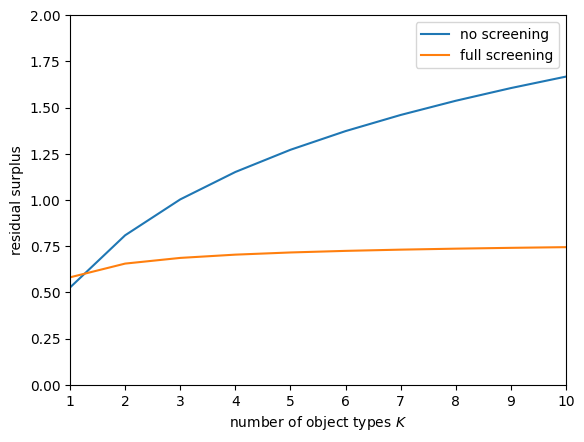
Figure B.8: The performance of no screening and full screening when the marginal value distribution $G$ is Weibull with shape parameter $0.9$.

Finally, we depict the performance of a no-screening mechanism and full-screening mechanism in Figure B.8. With small $K$, there is a substantially large region at which the hazard rate is still decreasing. Nevertheless, Figure B.8 indicates that a no-screening mechanism (e.g., SD) outperforms a full-screening mechanism (e.g., VCG) even with $K=2$, and the relative performance of no screening improves rapidly as $K$ increases.

B.2 Supplementary Materials for Section 3

This section illustrates how SD and VCG as an efficient mechanism in an i.i.d. environment looks like. We compare these with figures presented in Section B.2 for contrast. Specifically, we adopt Weibull with shape parameter $\alpha$ as the marginal value distribution. We illustrate two cases. In Figure B.9, we illustrate the case of $(\bar{m},\alpha)=(0.25,1.1)$, with which the marginal value distribution $G$ has an IHR, and thus SD is efficient for all $K\geq 1$. In Figure B.10, we depict the case of $(\bar{m},\alpha)=(0.25,0.5)$. In this case, for $K=2$, the reduced value distribution $G_{K}$ has a DHR, and VCG is an efficient mechanism.

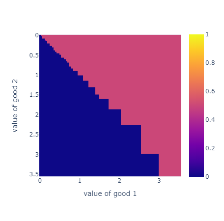
(a) $x_{1}(v_{1},v_{2})$

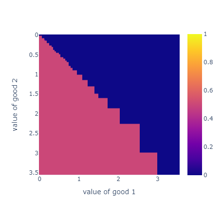
(b) $x_{2}(v_{1},v_{2})$

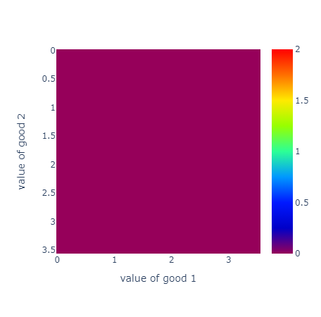
(c) $p(v_{1},v_{2})$

Figure B.9: An efficient mechanism for the case at which $G$ is Weibull with shape parameter $\alpha=1.1$, and $\bar{m}=0.25$. This optimal solution can be achieved by SD.

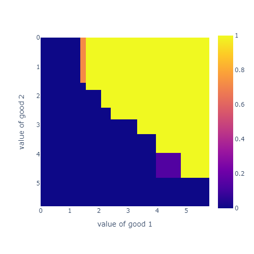
(a) $x_{1}(v_{1},v_{2})$

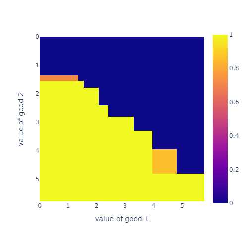
(b) $x_{2}(v_{1},v_{2})$

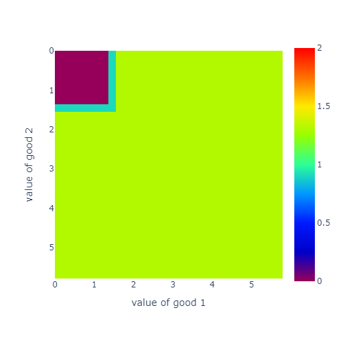
(c) $p(v_{1},v_{2})$

Figure B.10: An efficient mechanism for the case at which $G$ is Weibull with a shape parameter $\alpha=0.5$, and $\bar{m}=0.25$. This optimal solution can be achieved by VCG.

In Figure B.9, SD is shown as an efficient mechanism. No agent makes payment, and the allocation probability is independent of agents’ values (i.e., preference intensity) conditional on the preference order. By contrast, Figure B.10 concretely exhibits VCG’s property: Each agent is assigned only when their value is higher than a threshold (roughly $1.3$).

B.3 Supplementary Materials for Section 4

(a) Case (iii): $x_{1}^{1}(v_{1}^{1},v_{2}^{1},2,1)$

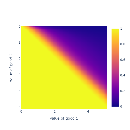
(b) Case (iii): $x_{2}^{1}(v_{1}^{1},v_{2}^{1},2,1)$

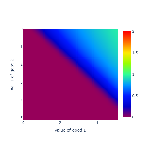
(c) Case (iii): $p^{1}(v_{1}^{1},v_{2}^{1},2,1)$

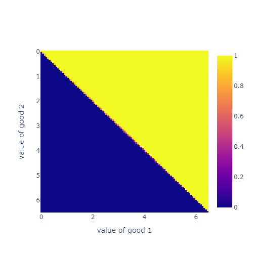
(d) Case (iv): $x_{1}^{1}(v_{1}^{1},v_{2}^{1},2,1)$

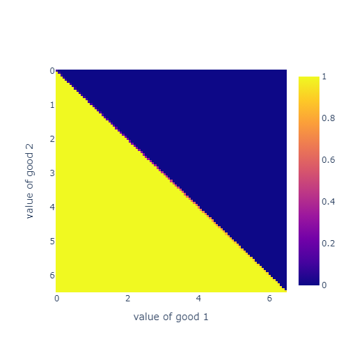
(e) Case (iv): $x_{2}^{1}(v_{1}^{1},v_{2}^{1},2,1)$

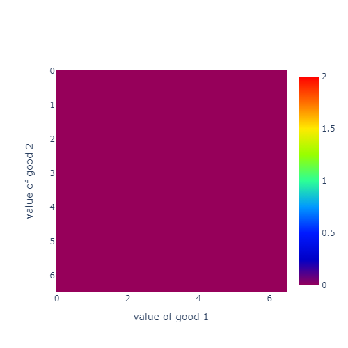
(f) Case (iv): $p^{1}(v_{1}^{1},v_{2}^{1},2,1)$

Figure B.11: Allocation and payment for agent 1 from an efficient mechanism learned by RegretNet for cases (iii) and (iv) in Section 4.2.3. Agent 2’s value is fixed to $(v^{2}_{1},v^{2}_{2})=(2,1)$. VCG is efficient for case (iii), whereas SD is efficient for case (iv).

Figures B.11 shows the mechanisms returned by RegretNet for cases (iii) and (iv) in Section 4.2.2. As shown in Panels (a), (b), and (c), in case (iii), RegretNet returns VCG as an efficient mechanism, although SD is the efficient mechanism in the corresponding i.i.d. case, case (i) in Section 4.2.2. Conversely, Panels (d), (e), and (c) demonstrate that, in case (iv), RegretNet returns SD as an efficient mechanism, whereas VCG is the efficient mechanism in the corresponding i.i.d. case.

References

- Abdulkadiroğlu et al. (2011) Abdulkadiroğlu, A., Y.-K. Che, and Y. Yasuda (2011): “Resolving Conflicting Preferences in School Choice: The “Boston Mechanism” Reconsidered,” American Economic Review, 101, 399–410.
- Abdulkadiroğlu et al. (2009) Abdulkadiroğlu, A., P. A. Pathak, and A. E. Roth (2009): “Strategy-Proofness Versus Efficiency in Matching with Indifferences: Redesigning the NYC High School Match,” American Economic Review, 99, 1954–1978.
- Abdulkadiroğlu and Sönmez (2003) Abdulkadiroğlu, A. and T. Sönmez (2003): “School Choice: A Mechanism Design Approach,” American Economic Review, 93, 729–747.
- Ahuja et al. (2021) Ahuja, A., S. Athey, A. Baker, E. Budish, J. C. Castillo, R. Glennerster, S. D. Kominers, M. Kremer, J. Lee, C. Prendergast, C. M. Snyder, A. Tabarrok, B. J. Tan, and W. Wiecek (2021): “Preparing for a Pandemic: Accelerating Vaccine Availability,” AEA Papers and Proceedings, 111, 331–35.
- Akbarpour et al. (2023) Akbarpour, M., E. Budish, P. Dworczak, and S. D. Kominers (2023): “An Economic Framework for Vaccine Prioritization,” Quarterly Journal of Economics, 139, 359–417.
- Asahi Shimbun (2021a) Asahi Shimbun (2021a): “Vaccine Reservations Overwhelming Phone Lines: Concerns of Nationwide Confusion,” Asahi Shimbun, in Japanese. Accessed: 2024-08-06.
- Asahi Shimbun (2021b) ——— (2021b): “Yokohama City Halts Vaccine Reservations: Overwhelming Access, Insufficient Response,” Asahi Shimbun, in Japanese. Accessed: 2024-08-06.
- Ashlagi and Shi (2016) Ashlagi, I. and P. Shi (2016): “Optimal Allocation Without Money: An Engineering Approach,” Management Science, 62, 1078–1097.
- Athey et al. (2022) Athey, S., J. C. Castillo, E. Chaudhuri, M. Kremer, A. Simoes Gomes, and C. M. Snyder (2022): “Expanding Capacity for Vaccines against COVID-19 and Future Pandemics: A Review of Economic Issues,” Oxford Review of Economic Policy, 38, 742–770.
- Bade (2015) Bade, S. (2015): “Serial Dictatorship: The Unique Optimal Allocation Rule when Information is Endogenous,” Theoretical Economics, 10, 385–410.
- Bogomolnaia and Moulin (2001) Bogomolnaia, A. and H. Moulin (2001): “A New Solution to the Random Assignment Problem,” Journal of Economic Theory, 100, 295–328.
- Castillo et al. (2021) Castillo, J. C., A. Ahuja, S. Athey, A. Baker, E. Budish, T. Chipty, R. Glennerster, S. D. Kominers, M. Kremer, G. Larson, J. Lee, C. Prendergast, C. M. Snyder, A. Tabarrok, B. J. Tan, and W. Wiecek (2021): “Market Design to Accelerate COVID-19 Vaccine Supply,” Science, 371, 1107–1109.
- Chakravarty and Kaplan (2013) Chakravarty, S. and T. R. Kaplan (2013): “Optimal Allocation without Transfer Payments,” Games and Economic Behavior, 77, 1–20.
- Che and Kojima (2010) Che, Y.-K. and F. Kojima (2010): “Asymptotic Equivalence of Probabilistic Serial and Random Priority Mechanisms,” Econometrica, 78, 1625–1672.
- Condorelli (2012) Condorelli, D. (2012): “What Money Can’t Buy: Efficient Mechanism Design with Costly Signals,” Games and Economic Behavior, 75, 613–624.
- Conitzer and Sandholm (2004) Conitzer, V. and T. Sandholm (2004): “Self-interested Automated Mechanism Design and Implications for Optimal Combinatorial Auctions,” in Proceedings of the 5th ACM Conference on Electronic Commerce, 132–141.
- Daskalakis et al. (2015) Daskalakis, C., A. Deckelbaum, and C. Tzamos (2015): “Strong Duality for a Multiple-Good Monopolist,” in Proceedings of the Sixteenth ACM Conference on Economics and Computation, 449–450.
- De Haan and Ferreira (2006) De Haan, L. and A. Ferreira (2006): Extreme Value Theory: An Introduction, vol. 3, Springer.
- Dütting et al. (2019) Dütting, P., Z. Feng, H. Narasimhan, D. Parkes, and S. S. Ravindranath (2019): “Optimal Auctions through Deep Learning,” in International Conference on Machine Learning, PMLR, 1706–1715.
- Fisher and Tippett (1928) Fisher, R. A. and L. H. C. Tippett (1928): “Limiting Forms of the Frequency Distribution of the Largest or Smallest Member of a Sample,” in Mathematical proceedings of the Cambridge philosophical society, Cambridge University Press, vol. 24, 180–190.
- Fotakis et al. (2016) Fotakis, D., D. Tsipras, C. Tzamos, and E. Zampetakis (2016): “Efficient Money Burning in General Domains,” Theory of Computing Systems, 59, 619–640.
- Fu (2017) Fu, H. (2017): “Notes on Myerson’s Revenue Optimal Mechanisms,” Lecture Note.
- Gans (2022) Gans, J. S. (2022): “Optimal Allocation of Vaccines in a Pandemic,” Oxford Review of Economic Policy, 38, 912–923.
- Giannakopoulos and Koutsoupias (2018) Giannakopoulos, Y. and E. Koutsoupias (2018): “Duality and Optimality of Auctions for Uniform Distributions,” SIAM Journal on Computing, 47, 121–165.
- Gnedenko (1943) Gnedenko, B. (1943): “Sur La Distribution Limite Du Terme Maximum D’Une Serie Aleatoire,” Annals of Mathematics, 44, 423–453.
- Goldner and Lundy (2024) Goldner, K. and T. Lundy (2024): “Simple Mechanisms for Utility Maximization: Approximating Welfare in the I.I.D. Unit-Demand Setting,” Working Paper.
- Gumbel (1958) Gumbel, E. J. (1958): Statistics of Extremes, Columbia University Press.
- Haghpanah and Hartline (2021) Haghpanah, N. and J. Hartline (2021): “When Is Pure Bundling Optimal?” Review of Economic Studies, 88, 1127–1156.
- Hakimov et al. (2021) Hakimov, R., C.-P. Heller, D. Kübler, and M. Kurino (2021): “How to Avoid Black Markets for Appointments with Online Booking Systems,” American Economic Review, 111, 2127–51.
- Hakimov et al. (2023) Hakimov, R., D. Kübler, and S. Pan (2023): “Costly Information Acquisition in Centralized Matching Markets,” Quantitative Economics, 14, 1447–1490.