Orbital Energies Are Chemical Potentials in Ground-State Density Functional Theory and Excited-State $\Delta$SCF Theory

Abstract

We prove the general chemical potential theorem: the noninteracting one-electron orbital energies in DFT ground states and $\Delta$SCF excited states are corresponding chemical potentials of electron addition or removal, from an $N$-particle ground or excited state to an $(N\pm 1)$-particle ground or excited state. This greatly extends the previous ground state results. Combining with the recently developed exact linear conditions for fractional charges in excited states, where the slopes of the linear lines are defined as the excited-state chemical potentials, our result establish the physical meaning of orbital energies as approximation to the corresponding excited-state ionization potentials and electron affinities, for both ground and excited states of a molecule or a bulk system. To examine the quality of this approximation we demonstrate numerically significant delocalization error in commonly used functionals and excellent agreement in functionals correcting the delocalization error.

Density functional theory (DFT) was formulated as a ground-state theory and has since become the primary tool for electronic structure calculations [1, 2, 3, 4, 5]. The accuracy of DFT computations hinges critically on the employed density functional approximations (DFAs). Developing improved functionals necessitates a deep understanding of the exact conditions they must fulfill [6, 7, 8, 9, 10, 11, 12].

The extension to fractional charges and the exact linear conditions for the energy were developed by Perdew, Parr, Levy and Baldus (PPLB) based on grand canonical ensembles [13, 14]. This led to the conclusion that the exact chemical potentials, as the derivative of total energy with respect to electron number has two limits for an integer particle system: it is equal to the negative of ionization potential (IP) on the electron removal side, and equal to the negative of electron affinity (EA) on the electron addition side [13]. The PPLB conditions were subsequently derived based on the exact properties of quantum mechanical degeneracy and size consistency [15], and extended to the combination of fractional charges and spins [16, 17]. The PPLB conditions play an important role in understanding the systematic errors in commonly used DFAs and in developing their corrections.

A major systematic error in DFAs is the delocalization error (DE) [18], which leads to the underestimation of band gaps, reaction barriers, binding energies of charge-transfer complexes, and dissociation energies, as well as the overestimation of polymer polarizabilities [19, 8, 20]. The DE has a size-dependent manifestation: for systems small both in number of atoms and in physical extent, DE appears as the convex deviation from the PPLB linearity conditions; but for large systems and bulk systems, DE leads to the incorrect total energy differences with the ($N\pm 1)$ charged states and consequently the underestimation of band gaps for bulk systems [18, 21]. To address these challenges, numerous correction methods have been proposed [22, 23, 24, 25, 26, 27, 28, 29, 30, 31, 32, 33, 34, 35, 36, 37, 38, 39, 40, 41, 21].

In the ground state KS theory, while the electron density is the basic but implicit variable, the noninteracting reference system provides the explicit variable for defining the kinetic and exchange-correlation energy functionals, and the electron density or the density matrix. The noninteracting reference system is associated with a noninteracting Hamiltonian, the eigenstates of which are the one-electron Kohn-Sham (KS) orbitals with corresponding orbital energies. The Janak theorem established the equality of orbital energies with the derivatives of total energy with respect to the orbital occupation numbers [42]. This is very important, but not directly connecting orbital energies to experimental observables. The physical meaning of the orbital energies is most interesting and has been explored over a long time from the conditions of the exact functional and exact asymptotic density behavior [43, 13, 44, 45], the connection with Dyson orbitals and ionization energies [46, 47], the observed approximation to optical excitation energies [48, 49], and the equality of frontier orbital energies with the chemical potentials (thus approximation to the ionization energy and electron affinity) [50, 8, 51].

In ground state DFT, two relationships connecting orbital energies to experimental observables have been established rigorously: (1) The ionization potential theorem [13]: For the exact and local Kohn-Sham potential, the KS highest occupied molecular orbital (HOMO) energy is negative of the first ionization energy [13, 44]. (2) The ground state chemical potential theorem [50]: In any ground-state DFA calculation with an $E_{xc}$ functional that is a continuous functional of density or the KS density matrix, the energy of the HOMO is the chemical potential of the electron removal and the energy of the lowest unoccupied molecular orbital (LUMO) is the chemical potential of electron addition [50, 8, 51]. The ground state chemical potential theorem justifies using the frontier orbital energies to approximate experimental IP and EA in molecules and valence and conduction band edge energies and hence band gaps in bulk systems, as the exact ground state chemical potentials are -IP and -EA from the PPLB condition [50, 8, 51]. The result is applicable both for the KS calculations with a local potential when the $E_{xc}$ is given as a functional of the density, and for the generalized KS calculation with a nonlocal potential when the $E_{xc}$ is given as a functional of the density matrix of the noninteracting reference system. Particularly, the ground state chemical potential theorem for the first time established the physical meaning of the LUMO energy in ground state (G)KS calculations, supported with numerical results [50, 51]. Further discussion for bulk systems can be found in Ref.[52].

The meaning of the other orbitals has also been much explored. For the occupied orbitals below HOMO, connections to the higher ionization energies has been discussed and observed in some DFA calculations with good agreement [46, 47]. For the unoccupied orbitals above LUMO, good agreement to the optical excitation energies was observed in atomic calculations with accurate KS local potentials [48], which was further explored [49].

Consistent with the ground-state chemical potential theorem, recent functional developments in reducing DE lead to results in excellent agreement of frontier orbital energies with the IP and EA in molecules, and band gaps for bulk systems, similar or better than the GW Green’s function results [50, 38, 39, 40, 53, 24, 26, 54, 34, 35, 55, 56, 57, 58, 59, 29, 60, 61]. Remarkably, similar agreements also have been reported for the energies of orbitals below HOMO with the negative of corresponding higher IPs [62], even for core orbitals [61], supporting the interpretation for all orbital energies as quasiparticle energies [62]. This quasiparticle energy interpretation is consistent with the IP and EA connection to the HOMO and LUMO energies and would present a unified physical meaning for the entire orbital spectrum, much like the Koopmans’ theorem for Hartree-Fock theory, under the frozen orbital assumption [63]. Furthermore, two groups have independently developed the method for calculating optical excitation energies of an $N$-particle system based on the ground state orbital energies of an $N-1$or $N+1$systems, using quasipaticle energies as approximated from the corresponding ground state orbital energies [64, 65, 62]. This method was called quasiparticle energy DFT (QE-DFT) and has been shown to describe well valence and Rydberg excitations [62], and charge transfer excitations [66], conical intersections [67] and excited-state charge transfer coupling [68].

For the quasiparticle energy interpretation of all orbital energies of a ground state to be true, the ground state DFT functional has to contain excited-state information. A abundance of accurate numerical results supports this interpretation [62, 61], but lacking a rigorous theoretical foundation. This motivated us to seek for the understanding, leading to the development of theoretical foundation for the $\Delta$SCF excited state approach [69], the extension of the excited state theory to fractional charges and the proof of the exact linear conditions [70], and the present work. The key result of present work is the establishment of the general chemical potential theorem on the physical meanings of all orbital energies, both for ground state (G)KS calculations while encompassing the previous ground state chemical potential theorem, and for excited state $\Delta$SCF calculations. Before we proceed, we need to review related developments in excited state theory.

Indeed, deviating from the ground-state formulation, KS DFT has been extensively employed for excited-state calculations via the $\Delta$SCF approach for a long time[71, 72]. It has demonstrated significant numerical success in predicting excitation energies [73, 74, 75, 76, 77, 78, 79, 80, 81, 82, 83, 84, 85, 86, 87, 88], albeit lacking a rigorous theoretical foundation [88], until recently [69].

To describe excited states, the electron density alone is insufficient. Instead, a set of equivalent variables defining the non-interacting reference system can be utilized: the excitation number $n_{s}$ and the local one-electron potential $w_{s}({\bf x})$, the noninteracting wavefunction $\Phi,$ or the 1-particle density matrix $\gamma_{s}({\bf x},{\bf x}^{\prime})$ [69]. While the electron density is no longer the fundamental variable, it remains crucial as the physical system’s density equals that of the non-interacting reference system for both ground states [1, 2, 3, 4] and excited states [69]. Ground and excited state energies and densities are obtained from the minimum and stationary solutions of the same universal functional.

Using $\gamma_{s}$ as the basic variable for describing excited states in the density matrix functional ($\gamma_{s}$FT) [69], the excited-state theory has been recently extended to fractional charges for excited states [70], following the previous approach for ground states [15]. Consider two many-electron systems with the same external potential $v(\mathbf{r})$, one with $N$ electron in the $n$th excited state, and the other with $N+1$ electrons in the $m$th excited state. The energies of these two states are $E_{v}^{n}(N)$ and $E_{v}^{m}(N+1)$ respectively. Within the $\Delta$SCF theory, as formulated recently, the corresponding non-interacting reference systems have the first-order density matrices $\gamma_{s}^{n_{s}}(N)$, and $\gamma_{s}^{m_{s}}(N+1)$ respectively, where $n_{s}$ and $m_{s}$ are the corresponding excitation numbers of the non-interacting reference systems [69]. Parallel to the ground state fractional charges in terms of electron densities, the fractional charge system for excited states is described by the density matrix, for $0\leq\delta\leq 1$,

$$\gamma_{s}=(1-\delta)\gamma_{s}^{n_{s}}(N)+\delta\gamma_{s}^{m_{s}}(N+1)$$ (1)

The following linear conditions has been proved for the exact energy functional [70]:

$$E_{v}[(1-\delta)\gamma_{s}^{n_{s}}(N)+\delta\gamma_{s}^{m_{s}}(N+1)]$$

$$= (1-\delta)E_{v}^{n}(N)+\delta E_{v}^{m}(N+1).$$ (2)

Note that the excited state excitation levels $n$ and $m$ correspond to the excitation levels $n_{s}$ and $m_{s}$ of the noninteracting reference system – they do not need to be the same [69]. This result agrees with PPLB linear conditions in the special case of ground states: $n_{s}=m_{s}=n=m=0.$ It extends the PPLB linear conditions in two key ways: the basic variables for the fractional charge systems are now $\gamma_{s},$ the 1-particle density matrices of the noninteracting reference systems, and the $N$- and $\left(N+1\right)$-electron states are all states, ground and excited.

For ground states, the PPLB linear conditions set the physical meaning for ground-state chemical potentials [89], $\mu=\left(\frac{\partial E_{v}(\mathit{\mathcal{N}})}{\partial\mathit{\mathcal{N}}}\right)_{v}$, the slopes of $E_{v}(\mathit{\mathcal{N}})$ ($\mathit{\mathcal{N}}$denotes fractional electron numbers): $\mu^{-}=-IP$ and $\mu^{+}=-EA$, where the ionization potential $IP=E_{v}(N-1)-E_{v}(N)$ and the electron affinity $EA=E_{v}(N)-E_{v}(N+1)$ [13, 3].

For excited states, the slopes of the linear curves in Eq. (2) also convey physical meanings. For a given $n_{s}$th eigenstate with an integer particle number $N,$ the fractional electron number $\mathit{\mathcal{N}}$ connecting to the $m_{s}$th eigenstate of the $(N+1)-$electron system (described by $\gamma_{s}^{m_{s}}(N+1)$) is $\mathit{\mathcal{N}}=(1-\delta)N+\delta(N+1)$, and the energy as a function of $\mathit{\mathcal{N}}$ is $E_{v}^{+}(n_{s},m_{s},\mathit{\mathcal{N}})=E_{v}[(1-\delta)\gamma_{s}^{n_{s}}(N)+\delta\gamma_{s}^{m_{s}}(N+1)],$ the left hand side of Eq. (2). The excited-state chemical potential $\mu_{n_{s}m_{s}}^{+}$ is the slope of $E_{v}^{+}(n_{s},m_{s},\mathit{\mathcal{N}})$: For $N\leq\mathcal{N}\leq N+1$,

$$\mu_{n_{s}m_{s}}^{+}(\mathcal{N})=\left(\frac{\partial E_{v}^{+}(n_{s},m_{s},\mathit{\mathcal{N}})}{\partial\mathit{\mathcal{N}}}\right)_{v}=E_{v}^{m}(N+1)-E_{v}^{n}(N).$$ (3)

Similarly on the electron removal side, the fractional electron number $\mathit{\mathcal{N}}$ connecting to the $l_{s}$th eigenstate of the $(N-1)-$electron system (described by $\gamma_{s}^{l_{s}}(N-1)$) is $\mathit{\mathcal{N}}=(1-\delta)N+\delta(N-1)$, and the energy as a function of $\mathit{\mathcal{N}}$ is $E_{v}^{-}(n_{s},l_{s},\mathit{\mathcal{N}})=E_{v}[(1-\delta)\gamma_{s}^{n_{s}}(N)+\delta\gamma_{s}^{l_{s}}(N-1)].$ The excited-state chemical potential $\mu_{n_{s}m_{s}}^{-}$ is the slope of $E_{v}^{-}(n_{s},l_{s},\mathit{\mathcal{N}})$: For $N-1\leq\mathcal{N}\leq N$,

$$\mu_{n_{s}l_{s}}^{-}(\mathcal{N})=\left(\frac{\partial E_{v}^{-}(n_{s},l_{s},\mathit{\mathcal{N}})}{\partial\mathit{\mathcal{N}}}\right)_{v}=E_{v}^{n}(N)-E_{v}^{l}(N-1).$$ (4)

There is an symmetry: $\mu_{n_{s}m_{s}}^{+}(N)$=$\mu_{m_{s}n_{s}}^{-}(N+1)$ [70]. For ground states, $\mu_{00}^{+}$ and $\mu_{00}^{-}$ agree with the chemical potentials, $\mu^{+}$ and $\mu^{-}$, from the PPLB condition [13, 3]. The excited-state chemical potentials are thus the negative of IP associated with an excited state with one electron removed as in Eq. (4), or the negative of EA associated with an excited state with one added electron as in Eq.(3).

Now we describe present work on the physical meaning of all orbital energies in $\Delta$SCF excited state theory for an $N$-particle ground or excited state. Consider a $\Delta$SCF calculation with a given DFA $E_{xc}[\gamma_{s}({\bf x},{\bf x}^{\prime})]$ for an excited state with fractional charge of Eq. (1), using fractional occupations of $0\leq f_{p}\leq 1,$

$$\gamma_{s}({\bf x},{\bf x}^{\prime})=\sum_{p}f_{p}\phi_{p}(\mathbf{x})\phi_{p}^{*}({\bf x}^{\prime}),$$ (5)

which is consistent with how fractional charge calculations are carried out in the ground-state (G)KS calculations ([72, 90, 91]. The total energy functional is

$$E_{v}\left[\gamma_{s}\right]=T_{s}\left[\gamma_{s}\right]+J\left[\rho\right]+E_{xc}[\gamma_{s}]+\int d\mathbf{r}v(\mathbf{x})\rho(\mathbf{x}),$$ (6)

where $T_{s}\left[\gamma_{s}\right]=\textrm{Tr}(t\gamma_{s})$ and $J\left[\rho\right]$ is the classical Coulomb interaction energy. The one-electron Hamiltonian for the nonintercating reference system is

$$h_{\text{eff}}({\bf x},{\bf x}^{\prime})=\frac{\delta E_{v}[\gamma_{s}]}{\delta\gamma_{s}(\mathbf{r}^{\prime},\mathbf{r})}=t+v_{\text{eff}}(\mathbf{x},\mathbf{x}^{\prime}),$$ (7)

where in general one has an effective nonlocal potential $v_{\text{eff}}(\mathbf{x},\mathbf{x}^{\prime})=\left(v(\mathbf{x})+v_{J}(\mathbf{r})\right)\delta(\mathbf{x}-\mathbf{x}^{\prime})+v_{xc}(\mathbf{x},\mathbf{x}^{\prime}),$with $v_{xc}(\mathbf{r},\mathbf{r}^{\prime})=\frac{\delta E_{xc}[\gamma_{s}]}{\delta\gamma_{s}(\mathbf{r}^{\prime},\mathbf{r})}$. When one uses a density functional approximation $E_{xc}[\rho]$, then $v_{xc}(\mathbf{x},\mathbf{x}^{\prime})=\frac{\delta E_{xc}[\rho]}{\delta\rho(\mathbf{r})}\delta(\mathbf{x},\mathbf{x}^{\prime})=v_{xc}(\mathbf{x})\delta(\mathbf{x},\mathbf{x}^{\prime})$.

Consider the derivative of the total energy with respect to the orbital occupation $f_{q}$,

$$\frac{\partial E_{v}\left[\gamma_{s}\right]}{\partial f_{q}} =\int d{\bf x}d{\bf x}^{\prime}\frac{\delta E_{v}[\gamma_{s}]}{\delta\gamma_{s}({\bf x},{\bf x}^{\prime})}\left(\frac{\partial\gamma_{s}({\bf x},{\bf x}^{\prime})}{\partial f_{q}}\right)$$

$$=\left\langle\phi_{q}\left|h_{\text{eff}}\right|\phi_{q}\right\rangle=\varepsilon_{q}$$ (8)

where we used $h_{\text{eff}}\left|\phi_{q}\right\rangle=\varepsilon_{q}\left|\phi_{q}\right\rangle$ which is satisfied upon SCF convergence and the fact that orbital derivative terms sum to zero: $\left\langle\phi_{p}\left|h_{\text{eff}}\right|\frac{\partial\phi_{p}}{\partial f_{q}}\right\rangle+\left\langle\frac{\partial\phi_{p}}{\partial f_{q}}\left|h_{\text{eff}}\right|\phi_{p}\right\rangle=\varepsilon_{p}\frac{\partial}{\partial f_{q}}\left\langle\phi_{p}\right|\left.\phi_{p}\right\rangle=0.$ Eq. (8) is a direct generalization of Janak’s result to $\Delta$SCF excited state theory for fractional particle numbers, and with extension for nonlocal potential GKS calculations (which was previously developed for ground states [19, 21]). It is thus valid for all orbitals with any fractional occupation, with local or nonlocal one-electron potential and for ground-state and excited state $\Delta$SCF calculations.

For a physical system with integer particle numbers in its $n$th excited state described by the $n_{s}$th excited state of of a noninteracting system in $\Delta$SCF approach, we consider the removal of an infinitesimal charge $\delta f_{i}$ from an occupied orbital $i$. This moves our system from the original $N$-particle excited state $n_{s}$ towards the $(N-1)$-particle excited state $l_{s}$, the associated chemical potential is

$$\mu_{n_{s}l_{s}}^{-}(N) =\left.\left(\frac{\partial E_{v}^{-}(n_{s},l_{s},\mathit{\mathcal{N}})}{\partial\mathit{\mathcal{N}}}\right)_{v}\right|_{f_{i}=1}$$

$$=\left.\frac{\partial E_{v}\left[\gamma_{s}\right]}{\partial f_{i}}\right|_{f_{i}=1}=\varepsilon_{i}(N),$$ (9)

which is just the orbital energy of the $i$th occupied state. Similarly for an unoccupied orbital $a$ ,

$$\mu_{n_{s}m_{s}}^{+}(N) =\left.\left(\frac{\partial E_{v}^{+}(n_{s},m_{s},\mathit{\mathcal{N}})}{\partial\mathit{\mathcal{N}}}\right)_{v}\right|_{f_{a}=0}$$

$$=\left.\frac{\partial E_{v}\left[\gamma_{s}\right]}{\partial f_{a}}\right|_{f_{a}=0}=\varepsilon_{a}(N).$$ (10)

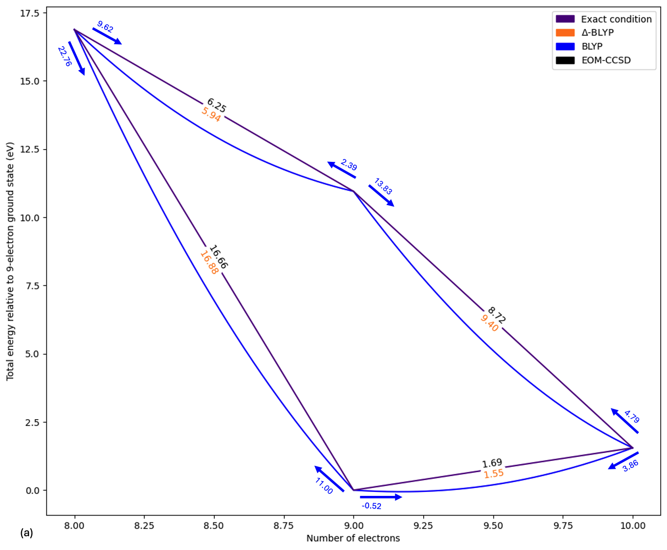
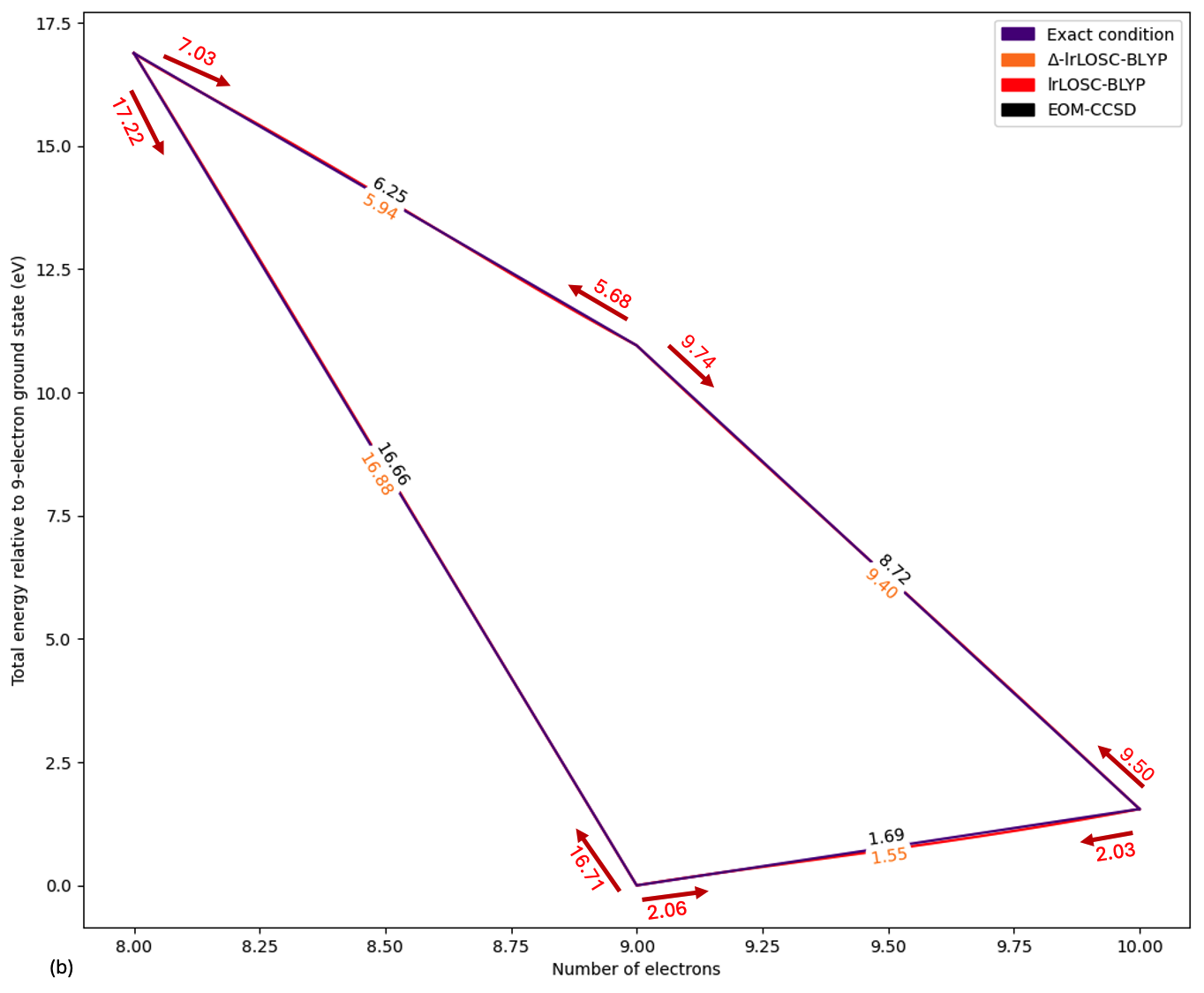
Figure 1: Excited-state energies for fractional charges and excited-state chemical potentials calculated from orbital energies in transitions between three systems in four states, $\text{OH}^{+}$ (N=8, excited state ${}^{3}\Pi$ ), OH (N=9, ground state ${}^{2}\Pi$ and excited state ${}^{4}\Pi$), and $\text{OH}^{-}$ (N=10, ${}^{3}\Pi$ excited state). Orbital energies for BLYP[92, 93] (a, blue) and lrLOSC-BLYP[40, 41, 94, 61, 60] (b, red) are shown with numbers and arrows indicating the + or the - sign for the corresponding chemical potentials. Additionally, $\Delta$-BLYP (a,orange), $\Delta$-lrLOSC-BLYP (b, orange)and the reference EOM-CCSD results (black) are shown as inline labels.

The initial and the final excitation levels, $n_{s}$, $l_{s}$ and $m_{s}$, are uniquely determined by the three sets of integer orbital occupations corresponding to the initial $N$electron state and the final $(N\mp 1)$ states, together with the spectrum of the corresponding three distinctive noninteracting Hamiltonians. Note that within $\Delta$SCF, each excited state of a physical system has its own inoninteracting reference system and a unique $h_{\text{eff}}$. While the orbital index $i$ for electron removal and $a$ for electron addition do not themselves explicitly lead to the excitation levels $l_{s}$ and $m_{s}$ for the final $(N\mp 1)$ states, they do so in combination with the spectrum of each $h_{\text{eff}}$. The symmetry relation in chemical potentials $\mu_{n_{s}m_{s}}^{+}(N)$=$\mu_{m_{s}n_{s}}^{-}(N+1)$ for the exact theory will also be reflected in the corresponding symmetry of orbital energies $\varepsilon_{a}(N)$ and $\varepsilon_{i}(N+1)$.

Eqs. (9-10), exact for any continuous (approximate) DFAs, are the key results of the general chemical potential theorem: It equates an occupied/unocxcupied orbital energy to the corresponding excited-state chemical potential of electron removal/addition. It greatly extends the previous results that are limited to all ground-state quantities [50]. With the exact conditions for excited-state chemical potentials, Eqs. (3-4), the orbital energies are thus the DFA approximation to the corresponding excited-state IP, or excited-state quasiparticle energy,

$$\varepsilon_{i}(N)=E_{v}^{n}(N)-E_{v}^{l}(N-1).$$ (11)

and excited-state EA, or excited-state quasiparticle energy,

$$\varepsilon_{a}(N)=E_{v}^{m}(N+1)-E_{v}^{n}(N).$$ (12)

When starting from a ground state, $n=n_{s}=0$, we have $\varepsilon_{i}(N)=E_{v}^{0}(N)-E_{v}^{l}(N-1),$ and $\varepsilon_{a}(N)=E_{v}^{m}(N+1)-E_{v}^{0}(N).$ This provides the theoretical foundation for the quasiparticle energy interpretation of all orbital energies of ground-state calculations and thus for using orbital energies in predicting photoemission and inverse photoemission spectra of ground state systems [62]. It also justifies the QE-DFT approach [64, 65, 62] to calculating optical excitation energies of an $N$-particle system from $(N\pm 1)$-particle ground-state orbital energies.

Before this work, no interpretation of the orbital energies had been reported for excited state $\Delta$SCF calculations. Eqs. (11-12), going beyond QE-DFT, provides a new approach, which we call excited state quasiparticle energy from DFT (exQE-DFT), to predicting excitation energies of the $(N\pm 1)$-particle excited states, from the orbital energies of an $N$-particle excited state $\Delta$SCF calculation, allowing efficient computational approach to broader excitations.

For optimized effective potential (OEP) calculations, the orbital energies are in general not equal to the chemical potentials for ground states [19] and similarly for excited states (See SI). The quality of the approximation of orbital energies to the corresponding excited-state IPs/EAs depends on the exchange-correlation energy functional approximations used, as expected from previous results for ground state quantities [19].

Molecular	Chemical				EOM-
Orbital	Potential	$\varepsilon_{\text{PBE}}$	$\varepsilon_{\text{lrLOSC-PBE}}$	$\Delta$-PBE	CCSD
$(\sigma_{\beta}^{*})^{0}$	$\mu_{{}^{2}\Pi,^{1}\Pi}^{+}$(13)	11.382	6.432	6.548	6.855
$(\sigma_{\beta}^{*})^{1}$	$\mu_{{}^{1}\Pi,^{2}\Pi}^{-}$(14)	1.934	6.269
$(\sigma_{\alpha}^{*})^{0}$	$\mu_{{}^{2}\Pi,^{3}\Pi}^{+}$(13)	13.492	8.377	8.410	8.656
$(\sigma_{\alpha}^{*})^{1}$	$\mu_{{}^{3}\Pi,^{2}\Pi}^{-}$(14)	3.506	8.150
$(\sigma_{\beta}^{*})^{0}$	$\mu_{{}^{2}\Sigma^{+},^{1}\Sigma^{+}}^{+}$(13)	18.364	14.287	13.853	14.165
$(\sigma_{\beta}^{*})^{1}$	$\mu_{{}^{1}\Sigma^{+},^{2}\Sigma^{+}}^{-}$(14)	9.039	13.882
$(\pi_{\beta})^{0}$	$\mu_{{}^{2}\Pi,^{1}\Sigma^{+}}^{+}$(13)	22.624	17.315	17.223	17.039
$(\pi_{\beta})^{1}$	$\mu_{{}^{1}\Sigma^{+},^{2}\Pi}^{-}$(14)	11.835	17.065

Table 1: Excited state chemical potentials for carbon monoxide (CO) in eV. The first column shows the relevant molecular orbital with its occupation number in super script. The chemical potentials are expressed with molecular term symbols to label the excited states involved, with the number of electrons in parenthesis to indicate the particle number in the $\Delta$SCF calculation. The table includes chemical potentials between the ground state (${}^{1}\Sigma^{+}$) and the excited states (${}^{1}\Pi,^{3}\Pi$) of CO and the ground state (${}^{2}\Sigma^{+}$) and the excited state (${}^{2}\Pi$) of $\text{CO}^{+}$. The spin purification [73, 78] has been applied to $\mu_{{}^{2}\Pi,^{1}\Pi}^{+}$ and $\mu_{{}^{1}\Pi,^{2}\Pi}^{-}$ in $\Delta$PBE[6] and orbital energy calculations. PBE has good agreement with EOM-CCSD for chemical potentials from $\Delta$SCF total energy differences but significant exDE for chemical potentials from orbital energies. lrLOSC-PBE [40, 41, 94, 61, 60] gives essentially the same good total energies as PBE (not listed), but excellent chemical potentials from orbital energies. lrLOSC-PBE orbital energies also approximately satisfy the exact symmetry, eg, $\mu_{{}^{2}\Pi,^{1}\Pi}^{+}(13)=6.432\approx\mu_{{}^{1}\Pi,^{2}\Pi}^{-}(14)=6.269$.

While Eqs. (9-10) are exact for any continuous (approximate) DFAs, how well Eqs. (11-12) are satisfied depends on the quality of the DFA. With commonly used DFAs, we numerically demonstrate significant excited-state delocalization error (exDE) [70], in Figure 1, Table 1 and SI with many more systems. For small systems, DFAs have good description of the total excitation energies at integer charges and exDE is reflected in the significant and systematic convex deviation from exact linear lines for fractional charges proven recently [70], and the underestimation/overestimation of excited state IPs/EAs from orbital energies, similarly to ground states[19]. Based on the ground state understanding [18], we expect the underestimation/overestimation of excited state IPs/EAs from orbital energies will persist as systems get larger and approach the bulk limit: Even though the convex deviation from the linear conditions will decrease and disappear, exDE will manifest as the errors in the $\Delta$SCF excited state total energy differences. With functionals correcting DE (LOSC [40, 41, 94, 61, 60]) we show excellent agreement of excited state IPs/EAs with orbital energies from excited-state $\Delta$SCF calculations.

Our numerical results exemplify the general chemical potential theorem established in present work on the physical meaning of energies of all orbitals, occupied and virtual, for all states, ground and excited.

We acknowledge support from the National Science Foundation (CHE-2154831) and the National Institute of Health (R01-GM061870).

References

- Hohenberg and Kohn [1964] P. Hohenberg and W. Kohn, Inhomogeneous Electron Gas, Physical Review 136, B864 (1964).
- Kohn and Sham [1965] W. Kohn and L. J. Sham, Self-Consistent Equations Including Exchange and Correlation Effects, Physical Review 140, A1133 (1965).
- Parr and Yang [1989] R. G. Parr and W. Yang, Density-Functional Theory of Atoms and Molecules (Oxford University Press, New York, 1989).
- Dreizler and Gross [1990] R. M. Dreizler and E. K. U. Gross, Density functional theory: an approach to the quantum many-body problem (Springer, Berlin Heidelberg, 1990).
- M. Teale et al. [2022] A. M. Teale, T. Helgaker, A. Savin, C. Adamo, B. Aradi, A. V. Arbuznikov, P. W. Ayers, E. Jan Baerends, V. Barone, P. Calaminici, E. Cancès, E. A. Carter, P. Kumar Chattaraj, H. Chermette, I. Ciofini, T. Daniel Crawford, F. D. Proft, J. F. Dobson, C. Draxl, T. Frauenheim, E. Fromager, P. Fuentealba, L. Gagliardi, G. Galli, J. Gao, P. Geerlings, N. Gidopoulos, P. M. W. Gill, P. Gori-Giorgi, A. Görling, T. Gould, S. Grimme, O. Gritsenko, H. J. Aagaard Jensen, E. R. Johnson, R. O. Jones, M. Kaupp, A. M. Köster, L. Kronik, A. I. Krylov, S. Kvaal, A. Laestadius, M. Levy, M. Lewin, S. Liu, P.-F. Loos, N. T. Maitra, F. Neese, J. P. Perdew, K. Pernal, P. Pernot, P. Piecuch, E. Rebolini, L. Reining, P. Romaniello, A. Ruzsinszky, D. R. Salahub, M. Scheffler, P. Schwerdtfeger, V. N. Staroverov, J. Sun, E. Tellgren, D. J. Tozer, S. B. Trickey, C. A. Ullrich, A. Vela, G. Vignale, T. A. Wesolowski, X. Xu, and W. Yang, DFT exchange: Sharing perspectives on the workhorse of quantum chemistry and materials science, Physical Chemistry Chemical Physics , 28700 (2022).
- Perdew et al. [1996] J. P. Perdew, K. Burke, and M. Ernzerhof, Generalized gradient approximation made simple, Physical Review Letters 77, 3865 (1996).
- Burke [2012] K. Burke, Perspective on density functional theory, Journal of Chemical Physics 136, 150901 (2012).
- Cohen et al. [2012] A. J. Cohen, P. Mori-Sánchez, and W. Yang, Challenges for Density Functional Theory, Chemical Reviews 112, 289 (2012).
- Becke [2014] A. D. Becke, Perspective: Fifty years of density-functional theory in chemical physics, The Journal of Chemical Physics 140, 18A301 (2014).
- Sun et al. [2015] J. Sun, A. Ruzsinszky, and J. P. Perdew, Strongly Constrained and Appropriately Normed Semilocal Density Functional, Physical Review Letters 115, 036402 (2015).
- Wang et al. [2020] Y. Wang, P. Verma, L. Zhang, Y. Li, Z. Liu, D. G. Truhlar, and X. He, M06-SX screened-exchange density functional for chemistry and solid-state physics, Proceedings of the National Academy of Sciences 117, 2294 (2020).
- Mardirossian and Head-Gordon [2016] N. Mardirossian and M. Head-Gordon, omega B97M-V: A combinatorially optimized, range-separated hybrid, meta-GGA density functional with VV10 nonlocal correlation, Journal of Chemical Physics 144, 214110 (2016).
- Perdew et al. [1982] J. Perdew, R. Parr, M. Levy, and J. Balduz, Density-Functional Theory for Fractional Particle Number - Derivative Discontinuities of the Energy, Physical Review Letters 49, 1691 (1982).
- Zhang and Yang [2000] Y. Zhang and W. Yang, Perspective on ”Density-functional theory for fractional particle number: derivative discontinuities of the energy”, Theoretical Chemistry Accounts: Theory, Computation, and Modeling (Theoretica Chimica Acta) 103, 346 (2000).
- Yang et al. [2000] W. Yang, Y. Zhang, and P. W. Ayers, Degenerate ground states and a fractional number of electrons in density and reduced density matrix functional theory, Physical Review Letters 84, 5172 (2000).
- Cohen et al. [2008a] A. J. Cohen, P. Mori-Sánchez, and W. Yang, Fractional spins and static correlation error in density functional theory, The Journal of Chemical Physics 129, 121104 (2008a).
- Mori-Sánchez et al. [2009] P. Mori-Sánchez, A. J. Cohen, and W. Yang, Discontinuous Nature of the Exchange-Correlation Functional in Strongly Correlated Systems, Physical Review Letters 102, 066403 (2009).
- Mori-Sánchez et al. [2008] P. Mori-Sánchez, A. J. Cohen, and W. Yang, Localization and Delocalization Errors in Density Functional Theory and Implications for Band-Gap Prediction, Physical Review Letters 100, 146401 (2008).
- Cohen et al. [2008b] A. J. Cohen, P. Mori-Sanchez, and W. Yang, Insights into Current Limitations of Density Functional Theory, Science 321, 792 (2008b).
- Bryenton et al. [2022] K. R. Bryenton, A. A. Adeleke, S. G. Dale, and E. R. Johnson, Delocalization error: The greatest outstanding challenge in density-functional theory, Wiley Interdisciplinary Reviews-Computational Molecular Science 13, e1631 (2022).
- Mei et al. [2022] Y. Mei, J. Yu, Z. Chen, N. Q. Su, and W. Yang, LibSC: Library for Scaling Correction Methods in Density Functional Theory, Journal of Chemical Theory and Computation 18, 840 (2022).
- Perdew and Zunger [1981] J. Perdew and A. Zunger, Self-Interaction Correction to Density-Functional Approximations for Many-Electron Systems, Physical Review B 23, 5048 (1981).
- Pederson et al. [2014] M. R. Pederson, A. Ruzsinszky, and J. P. Perdew, Communication: Self-interaction correction with unitary invariance in density functional theory, Journal of Chemical Physics 140, 121103 (2014).
- Savin [1996] A. Savin, On degeneracy, near-degeneracy and density functional theory, in Theoretical and Computational Chemistry, Vol. 4 (Elsevier, 1996) pp. 327–357.
- Iikura et al. [2001] H. Iikura, T. Tsuneda, T. Yanai, and K. Hirao, A long-range correction scheme for generalized-gradient-approximation exchange functionals, The Journal of Chemical Physics 115, 3540 (2001).
- Song et al. [2009] J.-W. Song, M. A. Watson, and K. Hirao, An improved long-range corrected hybrid functional with vanishing Hartree-Fock exchange at zero interelectronic distance, LC2gau-BOP, Journal of Chemical Physics 131, 144108 (2009).
- Wagle et al. [2021] K. Wagle, B. Santra, P. Bhattarai, C. Shahi, M. R. Pederson, K. A. Jackson, and J. P. Perdew, Self-interaction correction in water–ion clusters, The Journal of Chemical Physics 154, 094302 (2021).
- Baer et al. [2010] R. Baer, E. Livshits, and U. Salzner, Tuned range-separated hybrids in density functional theory, Annual Review of Physical Chemistry 61, 85 (2010).
- Wing et al. [2021] D. Wing, G. Ohad, J. B. Haber, M. R. Filip, S. E. Gant, J. B. Neaton, and L. Kronik, Band gaps of crystalline solids from Wannier-localization–based optimal tuning of a screened range-separated hybrid functional, Proceedings of the National Academy of Sciences 118, 10/gmt8wp (2021).
- Su et al. [2014] N. Q. Su, W. Yang, P. Mori-Sánchez, and X. Xu, Fractional Charge Behavior and Band Gap Predictions with the XYG3 Type of Doubly Hybrid Density Functionals, J. Phys. Chem. A 118, 9201 (2014).
- Su and Xu [2016] N. Q. Su and X. Xu, Second-Order Perturbation Theory for Fractional Occupation Systems: Applications to Ionization Potential and Electron Affinity Calculations, J. Chem. Theory Comput. 12, 2285 (2016).
- [32] J. Li and W. Yang, Chemical Potentials and the One-Electron Hamiltonian of the Second-Order Perturbation Theory from the Functional Derivative Approach, J. Phys. Chem. A 128, 4876.
- Anisimov and Kozhevnikov [2005] V. I. Anisimov and A. V. Kozhevnikov, Transition state method and Wannier functions, Physical Review B 72, 075125 (2005).
- Ma and Wang [2016] J. Ma and L.-W. Wang, Using Wannier functions to improve solid band gap predictions in density functional theory, Scientific Reports 6, 24924 (2016).
- Dabo et al. [2010] I. Dabo, A. Ferretti, N. Poilvert, Y. Li, N. Marzari, and M. Cococcioni, Koopmans’ condition for density-functional theory, Physical Review B 82, 115121 (2010).
- Colonna et al. [2022a] N. Colonna, R. De Gennaro, E. Linscott, and N. Marzari, Koopmans spectral functionals in periodic-boundary conditions, Journal of Chemical Theory and Computation 18 (2022a).
- Cohen et al. [2007] A. J. Cohen, P. Mori-Sánchez, and W. Yang, Development of exchange-correlation functionals with minimal many-electron self-interaction error, The Journal of Chemical Physics 126, 191109 (2007).
- Zheng et al. [2011] X. Zheng, A. J. Cohen, P. Mori-Sánchez, X. Hu, and W. Yang, Improving Band Gap Prediction in Density Functional Theory from Molecules to Solids, Physical Review Letters 107, 10.1103/PhysRevLett.107.026403 (2011).
- Li et al. [2015] C. Li, X. Zheng, A. J. Cohen, P. Mori-Sánchez, and W. Yang, Local Scaling Correction for Reducing Delocalization Error in Density Functional Approximations, Physical Review Letters 114, 053001 (2015).
- Li et al. [2018] C. Li, X. Zheng, N. Q. Su, and W. Yang, Localized orbital scaling correction for systematic elimination of delocalization error in density functional approximations, National Science Review 5, 203 (2018).
- Su et al. [2020a] N. Q. Su, A. Mahler, and W. Yang, Preserving Symmetry and Degeneracy in the Localized Orbital Scaling Correction Approach, The Journal of Physical Chemistry Letters 11, 1528 (2020a).
- Janak [1978] J. F. Janak, Proof that in density-functional theory, Physical Review B 18, 7165 (1978).
- Morrell et al. [1975] M. M. Morrell, R. G. Parr, and M. Levy, Calculation of ionization potentials from density matrices and natural functions, and the long-range behavior of natural orbitals and electron density, The Journal of Chemical Physics 62, 549 (1975).
- Perdew and Levy [1997] J. P. Perdew and M. Levy, Comment on “Significance of the highest occupied Kohn-Sham eigenvalue”, Physical Review B 56, 16021 (1997).
- Tozer and Handy [2000] D. J. Tozer and N. C. Handy, On the determination of excitation energies using density functional theory, Phys. Chem. Chem. Phys. 2, 2117 (2000).
- Chong et al. [2002] D. P. Chong, O. V. Gritsenko, and E. J. Baerends, Interpretation of the Kohn–Sham orbital energies as approximate vertical ionization potentials, The Journal of Chemical Physics 116, 1760 (2002).
- Gritsenko et al. [2003] O. V. Gritsenko, B. Braïda, and E. J. Baerends, Physical interpretation and evaluation of the Kohn-Sham and Dyson components of the -I relations between the Kohn-Sham orbital energies and the ionization potentials, The Journal of Chemical Physics 119, 1937 (2003).
- Savin et al. [1998] A. Savin, C. J. Umrigar, and X. Gonze, Relationship of Kohn-Sham eigenvalues to excitation energies, Chemical Physics Letters 288, 391 (1998).
- van Meer et al. [2014] R. van Meer, O. V. Gritsenko, and E. J. Baerends, Physical Meaning of Virtual Kohn–Sham Orbitals and Orbital Energies: An Ideal Basis for the Description of Molecular Excitations, Journal of Chemical Theory and Computation 10, 4432 (2014).
- Cohen et al. [2008c] A. J. Cohen, P. Mori-Sánchez, and W. Yang, Fractional charge perspective on the band gap in density-functional theory, Physical Review B 77, 115123 (2008c).
- Yang et al. [2012] W. Yang, A. J. Cohen, and P. Mori-Sánchez, Derivative discontinuity, bandgap and lowest unoccupied molecular orbital in density functional theory, The Journal of Chemical Physics 136, 204111 (2012).
- Perdew et al. [2017] J. P. Perdew, W. Yang, K. Burke, Z. Yang, E. K. U. Gross, M. Scheffler, G. E. Scuseria, T. M. Henderson, I. Y. Zhang, A. Ruzsinszky, H. Peng, J. Sun, E. Trushin, and A. Goerling, Understanding band gaps of solids in generalized Kohn-Sham theory, Proc. Natl. Acad. Sci. U. S. A. 114, 2801 (2017), 28265085 .
- Su et al. [2020b] N. Q. Su, A. Mahler, and W. Yang, Preserving symmetry and degeneracy in the localized orbital scaling correction approach, J. Phys. Chem. Lett. 11, 1528 (2020b).
- Hirao et al. [2021] K. Hirao, H.-S. Bae, J.-W. Song, and B. Chan, Koopmans’-Type Theorem in Kohn–Sham Theory with Optimally Tuned Long-Range-Corrected (LC) Functionals, The Journal of Physical Chemistry A 125, 3489 (2021).
- Borghi et al. [2014] G. Borghi, A. Ferretti, N. L. Nguyen, I. Dabo, and N. Marzari, Koopmans-compliant functionals and their performance against reference molecular data, Physical Review B 90, 075135 (2014).
- Colonna et al. [2018] N. Colonna, N. L. Nguyen, A. Ferretti, and N. Marzari, Screening in Orbital-Density-Dependent Functionals, Journal of Chemical Theory and Computation 14, 2549 (2018).
- Nguyen et al. [2018] N. L. Nguyen, N. Colonna, A. Ferretti, and N. Marzari, Koopmans-Compliant Spectral Functionals for Extended Systems, Physical Review X 8, 021051 (2018).
- Colonna et al. [2019] N. Colonna, N. L. Nguyen, A. Ferretti, and N. Marzari, Koopmans-Compliant Functionals and Potentials and Their Application to the GW100 Test Set, Journal of Chemical Theory and Computation 15, 1905 (2019).
- Colonna et al. [2022b] N. Colonna, R. De Gennaro, E. Linscott, and N. Marzari, Koopmans Spectral Functionals in Periodic Boundary Conditions, Journal of Chemical Theory and Computation 18, 5435 (2022b).
- Williams and Yang [2024] J. Z. Williams and W. Yang, Correcting Delocalization Error in Materials with Localized Orbitals and Linear-Response Screening (2024), arXiv:2406.07351 [cond-mat, physics:physics].
- Yu et al. [2024] J. Yu, Y. Mei, Z. Chen, and W. Yang, Accurate Prediction of Core Level Binding Energies from Ground-State Density Functional Calculations: The Importance of Localization and Screening (2024), arXiv:2406.06345 [physics].
- Mei et al. [2019] Y. Mei, C. Li, N. Q. Su, and W. Yang, Approximating Quasiparticle and Excitation Energies from Ground State Generalized Kohn–Sham Calculations, The Journal of Physical Chemistry A 123, 666 (2019).
- Koopmans [1934] T. Koopmans, Über die zuordnung von wellenfunktionen und eigenwerten zu den einzelnen elektronen eines atoms, Physica 1, 104 (1934).
- Haiduke and Bartlett [2018] R. L. A. Haiduke and R. J. Bartlett, Communication: Can excitation energies be obtained from orbital energies in a correlated orbital theory?, The Journal of Chemical Physics 149, 131101 (2018).
- Mei et al. [2018] Y. Mei, C. Li, N. Q. Su, and W. Yang, Approximating Quasiparticle and Excitation Energies from Ground State Generalized Kohn-Sham Calculations, arXiv:1810.09906 [physics] (2018), arXiv: 1810.09906.
- Mei and Yang [2019a] Y. Mei and W. Yang, Charge transfer excitation energies from ground state density functional theory calculations, The Journal of Chemical Physics 150, 144109 (2019a).
- Mei and Yang [2019b] Y. Mei and W. Yang, Excited-State Potential Energy Surfaces, Conical Intersections, and Analytical Gradients from Ground-State Density Functional Theory, The Journal of Physical Chemistry Letters , 2538 (2019b).
- Kuan et al. [2024] K.-Y. Kuan, S.-H. Yeh, W. Yang, and C.-P. Hsu, Excited-State Charge Transfer Coupling from Quasiparticle Energy Density Functional Theory, The Journal of Physical Chemistry Letters 15, 6126 (2024).
- Yang and Ayers [2024] W. Yang and P. W. Ayers, Foundation for the SCF Approach in Density Functional Theory (2024), arXiv:2403.04604.
- Yang and Fan [2024] W. Yang and Y. Fan, Fractional Charges, Linear Conditions and Chemical Potentials for Excited States in SCF Theory (2024), arXiv:2408.08443.
- Slater [1972] J. C. Slater, Statistical exchange-correlation in the self-consistent field, in Advances in quantum chemistry, Vol. 6, edited by P.-O. Löwdin (Academic Press, 1972) pp. 1–92.
- Slater and Wood [1970] J. C. Slater and J. H. Wood, Statistical exchange and the total energy of a crystal, International Journal of Quantum Chemistry 5, 3 (1970).
- Ziegler et al. [1977] T. Ziegler, A. Rauk, and E. J. Baerends, On the calculation of multiplet energies by the hartree-fock-slater method, Theoretica chimica acta 43, 261 (1977).
- Gavnholt et al. [2008] J. Gavnholt, T. Olsen, M. Engelund, and J. Schiøtz, self-consistent field method to obtain potential energy surfaces of excited molecules on surfaces, Physical Review B 78, 075441 (2008).
- Gilbert et al. [2008] A. T. B. Gilbert, N. A. Besley, and P. M. W. Gill, Self-consistent field calculations of excited states using the maximum overlap method (MOM), J. Phys. Chem. A 112, 13164 (2008).
- Besley et al. [2009] N. A. Besley, A. T. B. Gilbert, and P. M. W. Gill, Self-consistent-field calculations of core excited states, The Journal of Chemical Physics 130, 124308 (2009).
- Harbola and Samal [2009] M. K. Harbola and P. Samal, Time-independent excited-state density functional theory: study of 1s(2)2p(3)(S-4) and 1s(2)2p(3)(D-2) states of the boron isoelectronic series up to Ne5+, Journal of Physics B-Atomic Molecular and Optical Physics 42, 015003 (2009).
- Kowalczyk et al. [2011] T. Kowalczyk, S. R. Yost, and T. V. Voorhis, Assessment of the SCF density functional theory approach for electronic excitations in organic dyes, The Journal of Chemical Physics 134, 054128 (2011).
- Maurer and Reuter [2011] R. J. Maurer and K. Reuter, Assessing computationally efficient isomerization dynamics: SCF density-functional theory study of azobenzene molecular switching, The Journal of Chemical Physics 135, 224303 (2011).
- Maurer and Reuter [2013] R. J. Maurer and K. Reuter, Excited-state potential-energy surfaces of metal-adsorbed organic molecules from linear expansion -self-consistent field density-functional theory (SCF-DFT), The Journal of Chemical Physics 139, 014708 (2013).
- Seidu et al. [2015] I. Seidu, M. Krykunov, and T. Ziegler, Applications of time-dependent and time-independent density functional theory to rydberg transitions, The Journal of Physical Chemistry A 119, 5107 (2015).
- Ye et al. [2017] H.-Z. Ye, M. Welborn, N. D. Ricke, and T. Van Voorhis, -SCF: A direct energy-targeting method to mean-field excited states, The Journal of Chemical Physics 147, 214104 (2017).
- Hait and Head-Gordon [2020] D. Hait and M. Head-Gordon, Highly accurate prediction of core spectra of molecules at density functional theory cost: Attaining sub-electronvolt error from a restricted open-shell Kohn–Sham approach, The Journal of Physical Chemistry Letters 11, 775 (2020).
- Carter-Fenk and Herbert [2020] K. Carter-Fenk and J. M. Herbert, State-targeted energy projection: A simple and robust approach to orbital relaxation of non-aufbau self-consistent field solutions, Journal of Chemical Theory and Computation 16, 5067 (2020).
- Levi et al. [2020] G. Levi, A. V. Ivanov, and H. Jónsson, Variational calculations of excited states via direct optimization of the orbitals in DFT, Faraday Discussions 224, 448 (2020).
- Corzo et al. [2022] H. H. Corzo, A. Abou Taka, A. Pribram-Jones, and H. P. Hratchian, Using projection operators with maximum overlap methods to simplify challenging self-consistent field optimization, Journal of Computational Chemistry 43, 382 (2022).
- Kumar and Luber [2022] C. Kumar and S. Luber, Robust SCF calculations with direct energy functional minimization methods and STEP for molecules and materials, The Journal of Chemical Physics 156, 154104 (2022).
- Vandaele et al. [2022] E. Vandaele, M. Mališ, and S. Luber, The SCF method for non-adiabatic dynamics of systems in the liquid phase, The Journal of Chemical Physics 156, 130901 (2022).
- Parr et al. [1978] R. G. Parr, R. A. Donnelly, M. Levy, and W. E. Palke, Electronegativity: the density functional viewpoint, The Journal of Chemical Physics 68, 3801 (1978).
- Mori-Sánchez et al. [2006] P. Mori-Sánchez, A. J. Cohen, and W. Yang, Many-electron self-interaction error in approximate density functionals, The Journal of Chemical Physics 125, 201102 (2006).
- Ruzsinszky et al. [2006] A. Ruzsinszky, J. P. Perdew, G. I. Csonka, O. A. Vydrov, and G. E. Scuseria, Spurious fractional charge on dissociated atoms: Pervasive and resilient self-interaction error of common density functionals, Journal of Chemical Physics 125, 194112 (2006).
- Becke [1988] A. D. Becke, Density-functional exchange-energy approximation with correct asymptotic behavior, Phys. Rev. A 38, 3098 (1988).
- Lee et al. [1988] C. Lee, W. Yang, and R. G. Parr, Development of the colle-salvetti correlation-energy formula into a functional of the electron density, Phys. Rev. B 37, 785 (1988).
- Mei et al. [2021] Y. Mei, Z. Chen, and W. Yang, Exact second-order corrections and accurate quasiparticle energy calculations in density functional theory, J. Phys. Chem. Lett. 12, 7236 (2021).