Quantum Register Machine: Efficient Implementation of Quantum Recursive Programs

Abstract

Quantum recursive programming has been recently introduced for describing sophisticated and complicated quantum algorithms in a compact and elegant way. However, implementation of quantum recursion involves intricate interplay between quantum control flows and recursive procedure calls. In this paper, we aim at resolving this fundamental challenge and develop a series of techniques to efficiently implement quantum recursive programs. Our main contributions include:

1. We propose a notion of quantum register machine, the first purely quantum architecture (including an instruction set) that supports quantum control flows and recursive procedure calls at the same time.

2. Based on quantum register machine, we describe the first comprehensive implementation process of quantum recursive programs, including the compilation, the partial evaluation of quantum control flows, and the execution on the quantum register machine.

3. As a bonus, our efficient implementation of quantum recursive programs also offers automatic parallelisation of quantum algorithms. For implementing certain quantum algorithmic subroutine, like the widely used quantum multiplexor, we can even obtain exponential parallel speed-up (over the straightforward implementation) from this automatic parallelisation. This demonstrates that quantum recursive programming can be win-win for both modularity of programs and efficiency of their implementation.

1 Introduction

Recursion in classical programming languages enables programmers to conveniently describe complicated computations as compact programs. By allowing any procedure to call itself, a short static program text can generate (unbounded) long dynamic program execution [26]. In the context of quantum programming, recursion has been recently studied for similar reasons [73, 24, 75]. In particular, a language $\mathbf{RQC}^{++}$ was introduced in [73, 75] for recursively programmed quantum circuits and quantum algorithms. The expressive power of $\mathbf{RQC}^{++}$ has been demonstrated by various examples.

The aim of this paper is to study how quantum recursive programs can be efficiently implemented. We choose to consider quantum recursive programs described by the language $\mathbf{RQC}^{++}$ [75]. But we expect that the techniques developed in this paper can work for other quantum programming languages that support recursion.

In general, quantum recursion involves the interplay of the following two programming features:

• Quantum control flows (in particular, those defined by quantum if-statements [2, 74, 61, 15, 71]) that allow program executions to be in quantum superposition, controlled by some external quantum coin.

• Recursive procedure calls that allow a procedure to call itself with different classical parameters.

A good implementation of quantum recursive programs should support the above two features harmoniously. A better implementation should further be efficient.

1.1 Motivating Example: Quantum Multiplexor

…increase of efficiency always comes down to exploitation of structure …

Edsger W. Dijkstra [27]

To illustrate the basic idea of our implementation, let us start with an algorithmic subroutine called quantum multiplexor [62], and see how quantum recursive programs can benefit its description and implementation. Quantum multiplexor is used in a wide range of quantum algorithms, for example, linear combination of unitaries (LCU) [19, 13, 14, 42], Hamiltonian simulation [6, 7, 8, 47], quantum state preparation [3, 82, 83, 46], solving quantum linear system of equations [18]. Let $N=2^{n}$ and $[N]=\left\{0,1,\ldots,N-1\right\}$. A quantum multiplexor can be described by the unitary

$$U=\sum_{x\in[N]}\ket{x}\!\bra{x}\otimes U_{x}.$$ (1)

Here, every unitary $U_{x}$ can be described by a quantum circuit, or more generally, a quantum program, say $C_{x}$. The quantum multiplexor $U$ applies $U_{x}$, conditioned on the state $\ket{x}$ of the first $n$ qubits.

A straightforward implementation of $U$ is by applying a sequential products of $N$ controlled-$U_{x}$:

$$\prod_{x\in[N]}\Big{(}\ket{x}\!\bra{x}\otimes U_{x}+\sum_{y\neq x}\ket{y}\!\bra{y}\otimes\mathbbm{1}\Big{)}.$$ (2)

This implementation has time complexity $O\left\lparen\sum_{x\in[N]}T_{x}\right\rparen$, where $T_{x}$ is the time for executing $C_{x}$ (i.e., implementing $U_{x}$). On the other hand, there exists a more efficient parallel implementation [82, 83] of $U$, with parallel time complexity $O\left\lparen n+\max_{x\in[N]}T_{x}\right\rparen$, using rather involved constructions similar to the bucket-brigade quantum random access memories [31, 30, 35, 34]. This implementation achieves exponential parallel speed-up (with respect to $n$) over the straightforward one. The price for obtaining such efficiency is the manual design of rather low-level quantum circuits.

It is natural to ask if we can design at high-level and still obtain an efficient implementation. For this example of quantum multiplexor, the intuition is as follows. First, $U$ can be described by a high-level quantum recursive program $\mathcal{P}$, which encapsulates both the control structure in 1 and all programs $C_{x}$ for describing unitaries $U_{x}$. Then, by storing the program $\mathcal{P}$ in a quantum memory, we can design a quantum register machine (to be formally defined in this paper) that automatically exploits the structure of $\mathcal{P}$ and executes all $C_{x}$’s (i.e., implements all $U_{x}$’s) in quantum superposition, thereby outperforming the straightforward implementation that only sequentially executes $C_{x}$’s.

$$\begin{split}P_{\textup{main}}\left\lparen n\right\rparen\Leftarrow\ &\mathit{P}\left\lparen n,0\right\rparen\\ \mathit{P}\left\lparen k,x\right\rparen\Leftarrow\ &\mathbf{if}\ k=0\ \mathbf{then}\ Q[x]\\ &\mathbf{else}\\ &\ \ \mathbf{qif}\left[q\left[k\right]\right]\ \ket{0}\rightarrow\mathit{P}\left\lparen k-1,2x\right\rparen\\ &\qquad\quad\square\ \ \ket{1}\rightarrow\mathit{P}\left\lparen k-1,2x+1\right\rparen\\ &\ \ \mathbf{fiq}\\ &\mathbf{fi}\\ Q[0]\Leftarrow\ &C_{0}\\ \ldots&\\ Q[N-1]\Leftarrow\ &C_{N-1}.\end{split}$$

Figure 1: Quantum multiplexor as a quantum recursive program.

Let us make the above intuition more concrete, by describing $U$ in a quantum recursive program (in the language $\mathbf{RQC}^{++}$ [75], further explained in Section 2) as in Figure 1. Here, the main procedure $P_{\textup{main}}\left\lparen n\right\rparen$ describes $U$, and every $Q[x]$ (or their procedure body $C_{x}$) describes $U_{x}$. Procedure $\mathit{P}\left\lparen k,x\right\rparen$ recursively collects the control information $x$ using the quantum if-statement ($\mathbf{qif}$ statement) and calls $Q[x]$ when $k=0$. At this point, we only need to note that the program in Figure 1 involves the interplay of the quantum control flow (managed by the $\mathbf{qif}$ statement) and recursive procedure calls. The $\mathbf{qif}$ statement in $\mathit{P}\left\lparen k,x\right\rparen$ creates two quantum branches (in superposition): if $q[k]$ is in state $\ket{0}$, $\mathit{P}\left\lparen k-1,2x\right\rparen$ is called; if $q[k]$ is in state $\ket{1}$, $\mathit{P}\left\lparen k-1,2x+1\right\rparen$ is called.

If the program in Figure 1 is compiled and stored into a quantum memory, then a quantum register machine that supports quantum control flows and recursive procedure calls can run through the two quantum branches in superposition. The cost for executing the $\mathbf{qif}$ statement only depends on the quantum branch that takes longer running time. This will incur a final time complexity proportional to the maximum $\max_{x\in[N]}T_{x}$ (compared to the sum $\sum_{x\in[N]}T_{x}$ in the straightforward implementation) and lead to an exponential parallel speed-up, similar to [82, 83].

1.2 Main Contributions

1.2.1 Architecture: Quantum Register Machine

We propose a notion of quantum register machine, a purely quantum architecture that supports quantum control flows and procedure calls at the same time. Its storage components include a constant number of quantum registers (simply called registers in the sequel) and a quantum random access memory (QRAM). The QRAM stores both compiled quantum programs and quantum data. The machine operates on registers like a classical CPU, executing the compiled program by fetching instructions from the QRAM. The machine is also accompanied with a set of low-level instructions, each specifying operations to be carried out by the machine. We briefly explain how the quantum register machine handles the aforementioned two features as follows:

Handle quantum control flows: Inspired by the previous work [80] (which borrows ideas from the classical reversible architectures [28, 70, 5, 68]), we put the program counter into a quantum register, which can be in quantum superposition. However, existing techniques are not enough. The quantum control flows introduce a challenge known as the synchronisation problem [51, 12, 53, 44, 54, 63, 49, 72, 80], which we want the machine to automatically handle. Our solution is to use a partial evaluation of quantum control flows (to be explained soon) before execution, and design a few corresponding quantum registers and mechanisms to exploit the partial evaluation result at runtime.

Handle recursive procedure calls: We allocate a call stack in the QRAM, which can also be in quantum superposition. Stack operations are made reversible by borrowing techniques from the classical reversible computing (e.g., [4]). It is worth noting that at runtime, all quantum registers and the QRAM (which also stores the dynamic call stack) can be in an entangled quantum state.

1.2.2 Implementation: Compilation, Partial Evaluation and Execution

We propose a comprehensive process of implementing high-level quantum recursive programs (described in the language $\mathbf{RQC}^{++}$) on the quantum register machine. This includes the following three steps: the first two are purely classical and the last is quantum.

Step 1. Compilation (presented in Section 4): The high-level program in $\mathbf{RQC}^{++}$ is compiled into a low-level one described by instructions, together with a series of transformations. This step only depends on the program text and is independent of inputs.

Step 2. Partial evaluation (presented in Section 5): Given the classical inputs (often specifying the size of quantum inputs), the quantum control flow information of the compiled program is evaluated. This step is independent of quantum inputs.

Step 3. Execution (presented in Section 6): With the programs and partial evaluation results loaded into the QRAM, the quantum inputs are finally considered, and the compiled program is executed with the aid of the partial evaluation results.

1.2.3 Bonus: Automatic Parallelisation

We show that quantum recursive programming can be win-win for both modularity of programs (demonstrated in [75] via various examples) and efficiency of their implementation (realised in this paper). In particular, as a bonus, the efficient implementation (as briefly described in Section 1.2.2) also offers automatic parallelisation of quantum algorithms. For implementing certain quantum algorithmic subroutine, like the quantum multiplexor introduced in Section 1.1, we can obtain an exponential speed-up (over the straightforward implementation) from this automatic parallelisation, in terms of (classical and quantum) parallel time complexity. Here, the classical parallel time complexity is relevant because the partial evaluation (Step 2 in Section 1.2.2) will be performed by a classical parallel algorithm.

For implementing the quantum multiplexor, we obtain the following theorem from the automatic parallelisation, whose proof sketch is to be shown in Section 7.

Theorem 1 (Automatic parallelisation of quantum multiplexor).

Via the quantum register machine, the quantum multiplexor 1 with each $U_{x}$ consisting of $T_{x}$ elementary unitary gates can be implemented in (classical and quantum) parallel time complexity (i.e., circuit depth) $\widetilde{O}\left\lparen n\cdot\max_{x\in[N]}T_{x}+n^{2}\right\rparen$, where $\widetilde{O}\left\lparen\cdot\right\rparen$ hides logarithmic factors.

Although the complexity in Theorem 1 is slightly worse than that in [82, 83] by a factor of $\widetilde{O}(n)$, it is worth stressing that the parallelisation in Theorem 1 is obtained automatically. Our framework steps towards a top-down design of (parallel) efficient quantum algorithms: the programmer only needs to design the high-level quantum programs (like in Figure 1), and the parallelisation is automatically realised by our implementation based on the quantum register machine. Further comparison of Theorem 1 and [82, 83] is deferred to Section I.2.

1.3 Structure of the Paper

For convenience of the reader, in Section 2 we briefly review the language $\mathbf{RQC}^{++}$ [75] for describing quantum recursive programs. In Section 3, we introduce the notion of quantum register machine. In Section 4, we present the compilation of programs in $\mathbf{RQC}^{++}$ to low-level instructions. Then, in Section 5, we present the partial evaluation of quantum control flows on the compiled program. In Section 6, we present the execution on quantum register machine. Finally, in Section 7, we analyse the efficiency of implementing quantum recursive programs in our framework, and show how it offers automatic parallelisation. In Section 8 we discuss related work, and in Section 9 we conclude and discuss future topics.

For readability, further details of Sections 2, 3, 4, 5, 6 and 7 are deferred to Appendices A, B, C, D, E and F, respectively. Also, more examples of quantum recursive programs are provided in Appendix H, and further discussions on related work are presented in Appendix I.

2 Background on Quantum Recursive Programs

In this section, we briefly introduce the high-level language $\mathbf{RQC}^{++}$ for describing quantum recursive programs, defined in [75]. A more detailed introduction will be presented in Appendix A. The two key features of this language, compared to other existing quantum programming languages, are quantum control flows and recursive procedure calls, which together support the quantum recursion (different from classical recursion in quantum programs as considered in e.g., [71, 24]).

2.1 Syntax

The alphabet of $\mathbf{RQC}^{++}$ consists of: (a) Classical variables, often denoted by $x,x_{1},x_{2},\ldots$; (b) Quantum variables, often denoted by $q,q_{1},q_{2},\ldots$; (c) Procedure identifiers, often denoted by $P,Q,P_{1},P_{2},\ldots$; and (d) Elementary unitary gates and elementary classical arithmetic operators. A program in $\mathbf{RQC}^{++}$ typically describes a parameterised unitary, where classical variables are solely for specifying the control of programs. We use $\overline{x}=x_{1}\ldots x_{n}$ to denote a list of classical variables. Similar notations apply to quantum variables and procedure identifiers.

Variables can be simple or array variables. The notion of array is standard, e.g., if $x$ is an one-dimensional classical array, then $x[10]$ represents the $10^{\textup{th}}$ element in $x$. Array variables induce subscripted variables: e.g., for a quantum array $q$, $q[2y+z]$ is an element in $q$ with subscription $2y+z$. For simplicity of presentation, in this paper we only consider one-dimensional arrays, and requires that for any classical subscripted variable $x[t]$, the expression $t$ contains no more subscripted variables.

We also consider arrays of procedure and subscripted procedure identifiers, for which notations are similar to that for variables. Moreover, for any procedure identifier $P$, we correspond to it a classical variable $P.\mathit{ent}$, storing the entry address of the declaration of $P$. The value of $P.\mathit{ent}$ is determined after the program is compiled and loaded into the quantum memory.

The syntax of $\mathbf{RQC}^{++}$ is summarised in Figure 2.

$$\mathcal{P}= \ \left\{P_{1}\left\lparen\overline{u}_{1}\right\rparen\Leftarrow C_{1},...,P_{n}\left\lparen\overline{u}_{n}\right\rparen\Leftarrow C_{n}\right\}$$ Procedure declaration

$$C::= \ \mathbf{skip}\mid C_{1};C_{2}$$ Sequential composition

$$\mid\overline{x}:=\overline{t}$$ Classical assignment

$$\mid U\left[\overline{q}\right]$$ Quantum unitary gate

$$\mid P(\overline{t})$$ Procedure call

$$\mid\mathbf{if}\ b\ \mathbf{then}\ C_{1}\ \mathbf{else}\ C_{2}\ \mathbf{fi}$$ Classical if-statement

$$\mid\mathbf{while}\ b\ \mathbf{do}\ C\ \mathbf{od}$$ Classical loop

$$\mid\mathbf{begin}\ \mathbf{local}\ \overline{x}:=\overline{t};\ C\ \mathbf{end}$$ Local classical variable block

$$\mid\mathbf{qif}\left[q\right](\ket{0}\rightarrow C_{0})\square(\ket{1}\rightarrow C_{1})\mathbf{fiq}$$ Quantum if-statement

Figure 2: The syntax of quantum recursive programming language $\mathbf{RQC}^{++}$.

Here, a program is specified by $\mathcal{P}$, a set of procedure declarations, among which there is a main procedure $P_{\textup{main}}$. Each procedure declaration has the form $P(\overline{u})\Leftarrow C$, where $P$ is the procedure identifier, $\overline{u}$ is a list of formal parameters (which can be empty), and $C$ is the procedure body. The recursion is supported by that $C$ can contains $P$ itself. A statement $C$ is inductively defined, where $U$ represents an elementary unitary gate and $b$ represents a classical binary expression. We further explain as follows.

• The procedure call $P\left\lparen\overline{t}\right\rparen$ has a list of classical expressions $\overline{t}$ as its actual parameters.

• The block statement $\mathbf{begin}\ \mathbf{local}\ \overline{x}:=\overline{t};C\ \mathbf{end}$ temporarily initialises classical variables $\overline{x}$ with the values of $\overline{t}$ at the beginning of the block, and restores their old values at the end of the block.

• The unitary gate $U\left[\overline{q}\right]$ applies the elementary quantum gate $U$ on quantum variables $\overline{q}$.

• The quantum if-statement $\mathbf{qif}\left[q\right]\left\lparen\ket{0}\rightarrow C_{0}\right\rparen\square\left\lparen\ket{1}\rightarrow C_{1}\right\rparen\mathbf{fiq}$ executes $C_{i}$, conditioned on the external qubit variable $q$ (a.k.a., quantum coin): if $q$ is in state $\ket{0}$, then $C_{0}$ is executed; if $q$ is in state $\ket{1}$, then $C_{1}$ is executed. Its formal semantics is presented in Section 2.2. Unlike the classical if-statement where the control flow only runs through one of the two branches, the quantum control flows run through both quantum branches created by the $\mathbf{qif}$ statement, in superposition. Note that the superposition state is held in the composite system including $q$ and the quantum variables in $C_{0},C_{1}$.

2.2 Semantics

Now we briefly introduce the operational semantics of $\mathbf{RQC}^{++}$. We use $\left\lparen C,\sigma,\ket{\psi}\right\rparen$ to denote a configuration, where $C$ is the remaining statement to be executed or $C=\ \downarrow$ (standing for termination), $\sigma$ is the current classical state, and $\ket{\psi}$ is the current quantum state. The operational semantics is defined in terms of transitions between configurations of the form: $\left\lparen C,\sigma,\ket{\psi}\right\rparen\rightarrow\left\lparen C^{\prime},\sigma^{\prime},\ket{\psi^{\prime}}\right\rparen$.

For simplicity of presentation, we only show the most non-trivial transition rule (QIF) for the operational semantics in Figure 3. Other transition rules are rather standard and deferred to Section A.3. In the (QIF) rule, $\ket{0}_{q}$ and $\ket{1}_{q}$ corresponds to the two quantum branches, controlled by the external quantum coin $q$. As usual, $\rightarrow^{k}$ denotes the composition of $k$ copies of $\rightarrow$, and $\rightarrow^{*}=\bigcup_{k=0}^{\infty}\rightarrow^{k}$. Note that $\left\lparen C_{i},\sigma,\ket{\theta_{i}}\right\rparen$ are required to terminate in the same classical state $\sigma^{\prime}$ for both branches ($i=0,1$) to prevent classical variables from being in superposition. This requirement can be promised by Condition 2 later explained in Section 2.3.

The semantics of the $\mathbf{qif}$ statement is exactly a quantum multiplexor [62] with one control qubit $q$: if each $C_{i}$ describes a unitary $U_{i}$, then $\mathbf{qif}[q]\left\lparen\ket{0}\rightarrow C_{0}\right\rparen\square\left\lparen\ket{1}\rightarrow C_{1}\right\rparen\mathbf{fiq}$ describes the unitary $U_{0}\oplus U_{1}=\ket{0}\!\bra{0}_{q}\otimes U_{0}+\ket{1}\!\bra{1}_{q}\otimes U_{1}$.

$$(\textup{QIF})\qquad\frac{\ket{\psi}=\alpha_{0}\ket{0}_{q}\ket{\theta_{0}}+\alpha_{1}\ket{1}_{q}\ket{\theta_{1}},\qquad\left\lparen C_{i},\sigma,\ket{\theta_{i}}\right\rparen\rightarrow^{*}\left\lparen\downarrow,\sigma^{\prime},\ket{\theta_{i}^{\prime}}\right\rparen\ (i=0,1)}{\left\lparen\mathbf{qif}\left[q\right]\left\lparen\ket{0}\rightarrow C_{0}\right\rparen\square\left\lparen\ket{1}\rightarrow C_{1}\right\rparen\mathbf{fiq},\sigma,\ket{\psi}\right\rparen\rightarrow\left\lparen\downarrow,\sigma^{\prime},\alpha_{0}\ket{0}_{q}\ket{\theta_{0}^{\prime}}+\alpha_{1}\ket{1}_{q}\ket{\theta_{1}^{\prime}}\right\rparen}$$

Figure 3: Selected transition rule (QIF) for the operational semantics of $\mathbf{RQC}^{++}$.

2.3 Conditions for Well-Defined Semantics

A program following the syntax in Figure 2 is not yet guaranteed to have well-defined semantics. We present three conditions for the program to have well-defined semantics. All conditions are introduced so that the (QIF) rule can be properly applied.

The first condition guarantees that in every $\mathbf{qif}$ statement, the quantum coin $q$ is external. We use $\mathit{qv}\left\lparen C,\sigma\right\rparen$ to denote the quantum variables in statement $C$ with respect to a given classical state $\sigma$. Its precise definition is given in Section A.3.1.

Condition 1 (External quantum coin).

For any $P(\overline{u})\Leftarrow C\in\mathcal{P}$, any $\mathbf{qif}[q]\left\lparen\ket{0}\rightarrow C_{0}\right\rparen\square\left\lparen\ket{1}\rightarrow C_{1}\right\rparen\mathbf{fiq}$ appearing in $C$, and any classical state $\sigma$ (of concern), $q\notin\mathit{qv}\left\lparen C_{0},\sigma\right\rparen\cup\mathit{qv}\left\lparen C_{1},\sigma\right\rparen$.

The second condition says that in every $\mathbf{qif}$ statement, both quantum branches $C_{0},C_{1}$ contain no free changed (classical) variables. A classical variable is free if it is not declared as local variable. It is changed if it appears on the LHS of an assignment. We use $\mathit{fcv}\left\lparen C,\sigma\right\rparen$ to denote the free changed variables in statement $C$ with respect to a given classical state $\sigma$. Its precise definition is given in Section A.3.1. This condition is introduced because the (QIF) rule requires $\left\lparen C_{i},\sigma,\ket{\psi}\right\rparen$ to terminate in the same classical state $\sigma^{\prime}$ for both branches $i=0,1$.

Condition 2 (No free changed variables in the $\mathbf{qif}$ statements).

For any $P\left\lparen\overline{u}\right\rparen\Leftarrow C\in\mathcal{P}$, any $\mathbf{qif}[q]\left\lparen\ket{0}\rightarrow C_{0}\right\rparen\square\left\lparen\ket{1}\rightarrow C_{1}\right\rparen\mathbf{fiq}$ appearing in $C$, and any classical state $\sigma$ (of concern), $\mathit{fcv}\left\lparen C_{0},\sigma\right\rparen=\mathit{fcv}\left\lparen C_{1},\sigma\right\rparen=\emptyset$.

Condition 2 seems stronger than required. However, note that if both $C_{0}$ and $C_{1}$ make consistent changes to some free variables (which is the case when the (QIF) rule is applicable), then such changes actually do not need to be performed inside the $\mathbf{qif}$ statement and can be pulled out to satisfy Condition 2. Thus, Condition 2 is a fair condition to achieve in practice.

The third condition says that every procedure body contains no free changed variables. This condition is introduced to simplify the process of compilation, as it allows the procedure calls to be arbitrarily used together with the $\mathbf{qif}$ statements without violating Condition 2. It is also easy to achieve in practice.

Condition 3 (No free changed variables in procedure bodies).

For any $P\left\lparen\overline{u}\right\rparen\Leftarrow C\in\mathcal{P}$ and any classical state $\sigma$ (of concern), $\mathit{fcv}\left\lparen C,\sigma\right\rparen=\emptyset$.

3 Quantum Register Machine

Now we start to consider how to implement quantum recursive programs defined in the previous section. As the basis, let us introduce the notion of quantum register machine, an architecture that supports quantum control flows and recursive procedure calls at the same time. Unlike most existing quantum architectures that use classical controllers to implement quantum circuits, the quantum register machine stores quantum programs and data in a quantum random access memory (QRAM) and executes on quantum registers. Like a classical CPU, the machine works by repeatedly applying a fixed unitary $U_{\textup{cyc}}$ every instruction cycle, which consists of several stages, including fetching an instruction from the QRAM, decoding it and executing it by performing corresponding operations. To support quantum control flows, additional stages related to the partial evaluation are also needed.

In the following, we first explain quantum registers and QRAM, and then describe a low-level instruction set QINS (quantum instructions) for the quantum register machine.

3.1 Quantum Registers

The quantum register machine has a constant number of quantum registers (or simply, registers), each storing a quantum word composed of $L_{\textup{word}}$ (called word length) qubits. Registers are directly accessible. The machine can perform a series of elementary operations on registers, including word-level arithmetic operations (see also Section 3.3), each assumed to take time $T_{\textup{reg}}$. The precise definition of elementary operations are deferred to Section B.1.

Registers are grouped into two types: system and user registers. There are eight system registers. The first five are rather standard and borrowed from the classical reversible architectures [70, 28, 5, 68], as quantum unitaries are intrinsically reversible. We describe their classical effects as follows.

• Program counter $\mathit{pc}$ records the address of the current instruction.

• Instruction $\mathit{ins}$ records the current instruction.

• Branching offset $\mathit{br}$ records the offset of the address of the next instruction to go from $\mathit{pc}$. More specifically, if $\mathit{br}=0$, then the address of the next instruction will be $\mathit{pc}+1$. Otherwise, the address of the next instruction will be $\mathit{pc}+\mathit{br}$.

• Return offset $\mathit{ro}$ records the offset for $\mathit{br}$ in the return of a procedure call.

• Stack pointer $\mathit{sp}$ records the current topmost location of the call stack.

In contrast, the last three system registers are novelly introduced to support an efficient implementation of the $\mathbf{qif}$ statements. They are related to the qif table, a data structure generated by the partial evaluation of quantum control flows and used to support an efficient implementation of the $\mathbf{qif}$ statements. We briefly describe their classical effects as follows, and will explain further details in Sections 5 and 6.

• Qif table pointer $\mathit{qifv}$ records the current node in the qif table.

• Qif wait counter $\mathit{qifw}$ records the number of instruction cycles to wait at the current node in the qif table.

• Qif wait flag $\mathit{wait}$ records whether the current instruction cycle needs to be skipped.

We also set the initial values of theses registers: $\mathit{pc}$, $\mathit{sp}$ and $\mathit{qifv}$ are initialised to $\ket{j}$, where $j$ is the starting addresses of the main program, the call stack and the qif table, respectively. Other system and user registers are initialised to $\ket{0}$.

3.2 Quantum Random Access Memory

The quantum register machine has a quantum random access memory (QRAM) composed of $N_{\textup{QRAM}}$ memory locations, each storing a quantum word. The QRAM is not directly accessible. Like a classical memory, access to QRAM is by providing an address register specifying the address, and a target register to hold the information retrieved from the specified location. Unlike the classical case, the address register can be in quantum superposition, and registers can be entangled with the QRAM.

We assume the following two types of elementary QRAM accesses.

Definition 1 (Elementary QRAM accesses).

• QRAM (swap) load. This access performs the unitary $U_{\textup{ld}}(r,a,\mathit{mem})$ defined by the mapping:

  $$\ket{x}_{r}\ket{i}_{a}\ket{M}_{\mathit{mem}}\mapsto\ket{M_{i}}_{r}\ket{i}_{a}\ket{M_{0},\ldots,M_{i-1},x,M_{i+1},\ldots,M_{N_{\textup{QRAM}}-1}}_{\mathit{mem}},$$ (3)

  for all $x$, $i$ and $M=(M_{0},\ldots,M_{N_{\textup{QRAM}}-1})$. Here, $r$ is the target register, $a$ is the address register, and $\mathit{mem}$ is the QRAM.

• QRAM (xor) fetch. This access performs the unitary $U_{\textup{fet}}(r,a,\mathit{mem})$ defined by the mapping:

  $$\ket{x}_{r}\ket{i}_{a}\ket{M}_{\mathit{mem}}\mapsto\ket{x\oplus M_{i}}_{r}\ket{i}_{a}\ket{M}_{\mathit{mem}},$$ (4)

  for all $x,i,M$.

Moreover, we assume the controlled versions (controlled by a register) of elementary QRAM accesses are also elementary. Suppose every elementary QRAM access takes time $T_{\textup{QRAM}}$.

3.2.1 Layout of the QRAM

The QRAM in the quantum register machine stores both programs and data. In particular, it contains the following sections.

1. Program section stores the compiled program in a low-level language QINS (to be defined in Section 3.3).

2. Symbol table section stores the name of every variable and its corresponding address. Here, unlike in the classical case, the symbol table is used at runtime instead of compile time (see also Section C.3), because arrays in $\mathbf{RQC}^{++}$ are not declared with fixed size.

3. Variable section stores the classical and quantum variables.

4. Qif table section stores the qif table (to be defined in Section 5.2).

5. Stack section stores the call stack to handle the procedure calls. The stack is composed of multiple stack frames, each corresponding to a procedure call. A stack frame stores the actual parameters and return offset from the caller to the callee, and the local data used by the callee.

We visualise the quantum register machine and the layout of the QRAM in Figure 4.

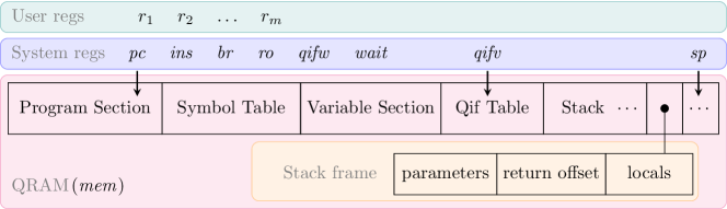
Figure 4: Storage components of the quantum register machine and the layout of the QRAM. All components can be together in a quantum superposition state.

3.3 The Low-Level Language QINS

Now we present QINS, a set of low-level instructions for describing the compiled programs. Each instruction specifies a series of elementary operations to be carried out by the quantum register machine. There are 22 instructions in QINS, which are listed with their classical effects in Figure 5(a). Here, we leave the explanation of instructions qif and fiq to Section 6. The classical effects of other instructions are lifted to quantum in the standard way when being executed by the quantum register machine.

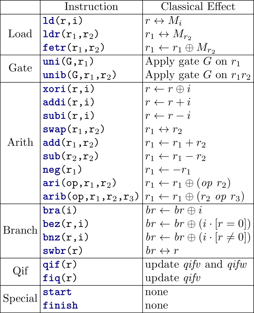
(a) Instructions and corresponding classical effects. Here, $\oplus$ denotes the XOR operator; $[b]=1$ if $b$ is true and $[b]=0$ otherwise.

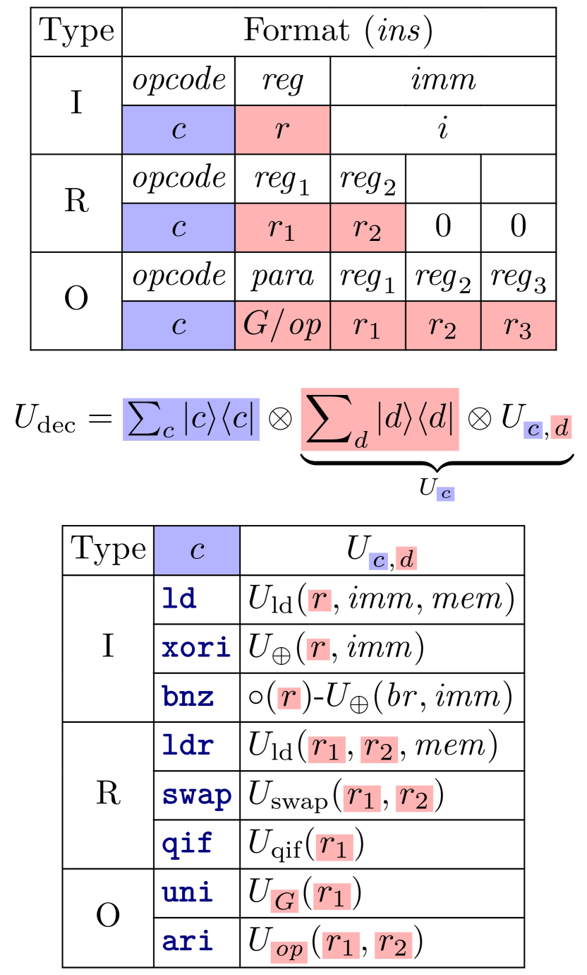
(b) Instruction formats, the decoding unitary $U_{\textup{dec}}$, and selected examples of instruction implementations.

Figure 5: The low-level language QINS and selected examples.

The design of QINS is inspired by the existing classical reversible instruction sets [28, 70, 5, 68]. Nevertheless, several instructions in QINS are essentially new. The most important are instructions qif and fiq, which are designed for a structured management of quantum control flows (generated by the $\mathbf{qif}$ statements in $\mathbf{RQC}^{++}$), in particular, aiding the partial evaluation and execution. Instructions uni and unib are designed for quantum unitary gates.

We group the instructions into three types: I (immediate-type), R (register-type) and O (other-type), according to their formats, as shown in Figure 5(b). In the execution on quantum register machine (to be described in Section 6), when we decode the instruction in register $\mathit{ins}$, we perform a unitary $U_{\textup{dec}}$, as shown in Figure 5(b). The unitary $U_{\textup{dec}}$ is a quantum multiplexor, with section $\mathit{opcode}$ as its first part of control (colored blue), and other sections (depending on the type I/R/O) in $\mathit{ins}$ as its second part of control (colored red). Let $c$ be a computational basis in the first part and $d$ in the second part, then the unitary being controlled is denoted by $U_{c,d}$.

For illustration, we select several instructions and their corresponding $U_{c,d}$ as examples in Figure 5(b). Here, $U_{\textup{ld}}$ is the QRAM access in Definition 1. $U_{\textup{qif}}$ (and similarly $U_{\textup{fiq}}$ for fiq) will be defined in Section 6. Other unitaries are elementary operations on registers: (a) $U_{\oplus}$ performs the mapping $\ket{x}\ket{y}\mapsto\ket{x\oplus y}\ket{y}$; (b) $\circ\left\lparen r\right\rparen$-$U$ stands for the controlled version $\ket{0}\!\bra{0}_{r}\otimes U+\sum_{x\neq 0}\ket{x}\!\bra{x}_{r}\otimes\mathbbm{1}$ of unitary $U$; (c) $U_{\textup{swap}}$ performs the mapping $\ket{x}\ket{y}\mapsto\ket{y}\ket{x}$; (d) $U_{G}$ applies the elementary gate $G$; (e) $U_{\mathit{op}}$ performs the mapping $\ket{x}\ket{y}\mapsto\ket{x\oplus\left\lparen\mathit{op}\ y\right\rparen}\ket{y}$ for unary operator $\mathit{op}$.

Further details of QINS are deferred to Section B.2.

4 Compilation

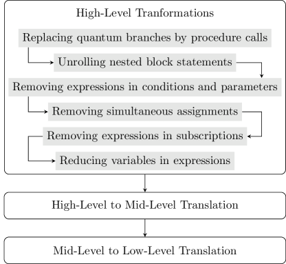
Figure 6: The compilation process.

As usual, the first step in the implementation of quantum recursive programs is their compilation. Roughly speaking, the compilation of a program $\mathcal{P}$ in $\mathbf{RQC}^{++}$ consists of the following passes.

1. First, a series of high-level transformations are performed on the original program $\mathcal{P}$, which simplify the program structure and make it easier to be further compiled. The transformed program $\mathcal{P}_{h}$ still follows the syntax of $\mathbf{RQC}^{++}$.

2. Then, the transformed program $\mathcal{P}_{h}$ is translated into an intermediate program $\mathcal{P}_{m}$ in the mid-level language composed of instructions similar to those in QINS but more flexible.

3. Finally, the mid-level $\mathcal{P}_{m}$ is translated into a program $\mathcal{P}_{l}$ in the low-level language QINS.

The compilation process is visualised in Figure 6. The remainder of this section is devoted to describe these passes carefully. In the sequel, we always assume the source program $\mathcal{P}$ to be compiled satisfies Conditions 1, 2 and 3 given in Section 2.3 and therefore has well-defined semantics.

4.1 High-Level Transformations

In this section, we describe the first pass of high-level transformation from $\mathcal{P}$ to $\mathcal{P}_{h}$. The major target of this pass is to simplify the automatic uncomputation of classical variables in later passes.

A program $\mathcal{P}$ in $\mathbf{RQC}^{++}$ may contain irreversible classical computations, e.g., classical assignment $x:=1$. Reversibly implementing irreversible statements introduces garbage data, e.g., through the standard Landauer [43] and Bennett [10] methods. For the overall correctness of the quantum computation, these garbage data should be properly uncomputed. Moreover, the block statement in $\mathbf{RQC}^{++}$ explicitly requires uncomputation of local variables at the end of the block.

$$\begin{split}&\mathbf{begin}\ \mathbf{local}\ x:=1;\\ &\ \ \mathbf{begin}\ \mathbf{local}\ y:=2x;\\ &\ \ \ \ x:=y+1;\\ &\ \ \ \ y:=2x\\ &\ \ \mathbf{end};\\ &\ \ U[q[x+2]]\\ &\mathbf{end}\end{split}$$

Figure 7: An example of nested block statement.

In the execution of a program, when should we perform uncomputation? First, we realise a difficulty from the uncomputation of local variables in nested block statements. Consider the example in Figure 7. The inner block changes the value of $x$, which is used by the outer block. If one tries to uncompute the local variable $y$ at the end of the inner block, the change on $x$ (by the inner block) is also uncomputed, which is an undesirable side effect.

To overcome this difficulty, we will perform a series of transformations on the original program $\mathcal{P}$, such that the transformed program $\mathcal{P}_{h}$ no longer contains nested block statements. Along the way, we also simplify the structure of the program. Consequently, for the program $\mathcal{P}_{h}$, we only need to perform uncomputation at the end of every procedure body (of procedure declarations), which will be automatically done in the high-level to mid-level translation (in Section 4.2).

An overview of high-level transformations is already shown in Figure 6. In the following we only select the first two steps for explanation, while other steps are rather standard (see e.g., the textbook [1]) and deferred to Section C.1.

4.1.1 Replacing Quantum Branches by Procedure Calls

In this step, we replace the program in every quantum branch of every $\mathbf{qif}$ statement by a procedure call. More specifically, for every $\mathbf{qif}$ statement, if $C_{0},C_{1}$ are not procedure identifiers or $\mathbf{skip}$ statements, then we introduce fresh procedure identifiers $P_{0},P_{1}$, perform the replacement:

$$\mathbf{qif}[q](\ket{0}\rightarrow C_{0})\square(\ket{1}\rightarrow C_{1})\mathbf{fiq}\qquad\Rightarrow\qquad\mathbf{qif}[q](\ket{0}\rightarrow P_{0})\square(\ket{1}\rightarrow P_{1})\mathbf{fiq},$$

and add new procedure declarations $P_{i}\Leftarrow C_{i}$ (for $i\in\left\{0,1\right\}$) to $\mathcal{P}$. If only one of $C_{0},C_{1}$ is procedure identifier or $\mathbf{skip}$, then the replacement is performed only for the other branch. It is easy to see the above transformation does not violate Conditions 1, 2 and 3.

4.1.2 Unrolling Nested Block Statements

In this step, we unroll all nested block statements. The program after this step is promised to no more contain block statements, but uncomputation of classical variables needs to be done at the end of every procedure body when the program is implemented, for it to preserve its original semantics. To do this, for any $P\left\lparen\overline{u}\right\rparen\Leftarrow C^{\prime}\in\mathcal{P}$ and every block statement appearing in $C^{\prime}$, we perform the replacement:

$$\mathbf{begin}\ \mathbf{local}\ \overline{x}:=\overline{t};\ C\ \mathbf{end}\qquad\Rightarrow\qquad\overline{x^{\prime}}:=\overline{x};C;\overline{x}:=\overline{x^{\prime}},$$

where $\overline{x^{\prime}}$ is a list of fresh variables. Also, we append $\overline{x^{\prime}}:=\overline{0}$ at the beginning of $C^{\prime}$. It is easy to see the above transformation keeps Conditions 1, 2 and 3 too.

Note that after this step, we actually slightly change the semantics of the language but preserves the semantics of the program, as long as uncomputation is done at the end of every procedure body when the program is implemented.

4.1.3 After the High-Level Transformations

We observe that the program $\mathcal{P}_{h}=\left\{P\left\lparen\overline{u}\right\rparen\Leftarrow C\right\}_{P}$ after the high-level transformations in Figure 6 has the following simplified syntax:

$$\begin{split}C::=&\ \mathbf{skip}\mid x:=t\mid U\left[\overline{q}\right]\mid C_{0};C_{1}\mid P(\overline{x})\mid\mathbf{if}\ x\ \mathbf{then}\ C_{0}\ \mathbf{else}\ C_{1}\ \mathbf{fi}\mid\mathbf{while}\ x\ \mathbf{do}\ C\ \mathbf{od}\\ &\mid\mathbf{qif}\left[q\right](\ket{0}\rightarrow P_{0})\square(\ket{1}\rightarrow P_{1})\mathbf{fiq},\end{split}$$

where every subscripted variable and procedure identifier has a basic classical variable as its subscription (e.g., $x[y]$), and every expression has the form $t\equiv\mathit{op}\ x$ or $t\equiv x\ \mathit{op}\ y$. As aforementioned, the semantics is slightly changed: uncomputation of classical variables are needed at the end of every procedure body in the implementation, (which will be automatically done in the high-level to mid-level translation in Section 4.2).

For illustration, on the LHS of Figure 8, we show an after-the-high-level-transformations version of the quantum multiplexor program in Figure 1. Note that some transformations have no effect on this example.

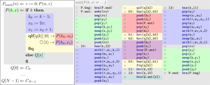
Figure 8: Example of high-level transformations and high-to-mid-level translation. The original program is the quantum multiplexor program in Figure 1. Here, on the LHS is the program after the high-level transformations. On the RHS is the high-to-mid-level translation of the procedure $P(k,x)$. Their connections are highlighted in colors.

4.2 High-Level to Mid-Level Translation

Now we translate the transformed high-level program $\mathcal{P}_{h}$ obtained in the previous subsection into $\mathcal{P}_{m}$ in a mid-level language, which is different from the low-level language QINS (defined in Section 3.3) in the following aspects:

• We do not consider the memory allocation. Thus, instructions ld, ldr and fetr are not needed at this stage.

• Beyond registers and numbers, instructions can also take variables and labels as input. Here, like in the classical assembly language, a label is an identifier for the address of an instruction. (When the program is further translated into QINS, in the next section, every label $l$ will be replaced by the offset of the address of where $l$ is defined from the address of where $l$ is used.)

• We have additional instructions push and pop for stack operations. Also, an additional branching instruction brc will be used in pair with bez (or bnz). In particular, brc(x,l), compared to bra(l), has the additional information of some variable $x$.

The high-to-mid-level translation also automatically handles the initialisation of formal parameters and the uncomputation of classical variables at the end of procedure bodies (see Section 4.1).

Let us use $\mathrm{mid}\left\{D\right\}$ to denote the high-to-mid-level translation of a statement (or declaration) $D$ in $\mathbf{RQC}^{++}$. In Figure 9, we present selected examples of the high-to-mid-level translation, and more details are deferred to Section C.2. Here, $\mathrm{init}\left\{\cdot\right\}$ and $\mathrm{uncp}\left\{\cdot\right\}$ denote the initialisation of formal parameters and uncomputation of classical variables, respectively. We further explain them as follows.

• To reversibly implement $\mathbf{while}\ x\ \mathbf{do}\ C\ \mathbf{od}$, a fresh variable $y$ is introduced to count the number of loops. Similar to the classical reversible architectures [70, 28, 5, 68], we use a pair of branching instructions (e.g., bnz and brc) to realise reversible (conditional) branching.

• In the translation of $\mathbf{qif}[q]\left\lparen\ket{0}\rightarrow C_{0}\right\rparen\square\left\lparen\ket{1}\rightarrow C_{1}\right\rparen\mathbf{fiq}$, we have a pair of instructions qif(q) and fiq(q), which indicate the creation and join of quantum branching, respectively. They will be used in the partial evaluation of quantum control flows and the final execution.

• The translations of procedure call $P\left\lparen\overline{x}\right\rparen$ and declaration $P\left\lparen\overline{u}\right\rparen\Leftarrow C$ are inspired by their counterparts in classical reversible computing [4]. Here, the biggest difference is our design of the automatic uncomputation of classical variables, performed by the program $\mathrm{uncp}\left\{C\right\}$ at the end of procedure body $C$ (see also Section 4.1.2), which reverses the changes on classical variables in $C$. The uncomputation $\mathrm{uncp}\left\{\cdot\right\}$ is also recursively defined, where $\mathrm{uncp}\left\{P\left\lparen\overline{x}\right\rparen\right\}$ and $\mathrm{uncp}\left\{\mathbf{qif}\ldots\mathbf{fiq}\right\}$ are set to empty, due to Conditions 3 and 2.

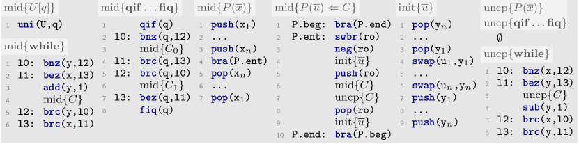
Figure 9: Selected examples of the high-to-mid-level translation. Here, $\mathrm{init}\left\{\cdot\right\}$ and $\mathrm{uncp}\left\{\cdot\right\}$ stand for the initialisation of formal parameters and uncomputation of classical variables, respectively. $y,y_{1},\ldots,y_{n}$ are all fresh variables. Also, $\mathrm{mid}\left\{\mathbf{while}\right\}$ and $\mathrm{uncp}\left\{\mathbf{while}\right\}$ use the same fresh variable $y$.

For illustration, on the RHS of Figure 8, we present an example of the high-to-mid-level translation of the quantum multiplexor program. For simplicity, we only show the translation of the recursive procedure $P(k,x)$. The full translation is deferred to Section C.2.

4.3 Mid-Level to Low-Level Translation

Now we are ready to describe the last pass in which the mid-level program $\mathcal{P}_{m}$ obtained in the previous sections is translated into a program $\mathcal{P}_{l}$ in the low-level language QINS and thus executable on the quantum register machine. In this pass, instructions that take variables and labels as inputs will be translated to instructions that only take registers and immediate numbers as inputs. The additional instructions push, pop and brc also need to be translated. To do this, we need the load instructions ld, ldr and fetr. Let us use $\mathrm{low}\left\{i\right\}$ to denote the mid-to-low-level translation of an instruction $i$. In Figure 10, we present selected examples of the mid-to-low-level translation, and more details are deferred to Section C.4. We further explain them as follows.

• The translation of uni(U,q[x]) shows how to handle inputs containing subscripted quantum variables. We use $@x$ to denote the address of the name $x$ (in the symbol table section of the QRAM; see Section 3.2.1). The word at $@x$ stores the address $\&x$ of the variable $x$ (in the variable section). Lines 1–2 load the value of $x$ into free register $r_{2}$. To obtain the address of $q[x]$, we add the address $\&q=\&\left\lparen q[0]\right\rparen$ and the value of $x$, in Lines 3–4. Line 5 loads the value of $q[x]$ into free register $r_{4}$, on which the instruction uni(U,r₄) is executed. Lines 7–11 reverse the effects of Lines 1-5. Further details of the symbol table and memory allocation of variables are deferred to Section C.3.

• In the translation of bra(P.ent), recall that the classical variable $P.\mathit{ent}$ corresponds to some procedure identifier $P$. Here, Lines 1–3 loads the value of $P.\mathit{ent}$ into free register $r_{2}$. Note that Line 2 uses fetr instead of ldr to preserve the copy of $P.\mathit{ent}$ in the QRAM for recursive procedure calls. Lines 4–5 calculate in $r_{2}$ the offset of $P.\mathit{ent}$ from the address of Line 6. When the branching occurs after Line 6, note that registers $r_{1}$ and $r_{2}$ are cleared. Lines 7–12 are similar.

• The translations of push and pop are rather simple. Note that they are reversible, e.g., if an element is pushed into the stack, the original register $r$ will be cleared.

• The translations of bez and brc are related when they are used in pairs: they use the same free registers $r_{1}$ and $r_{2}$.

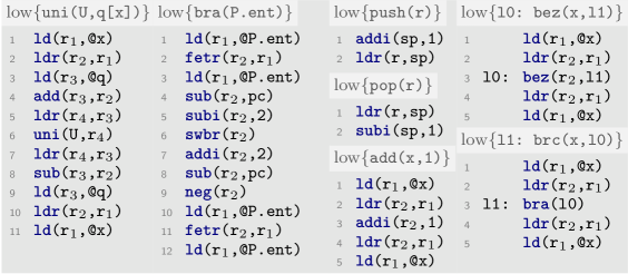
Figure 10: Selected examples of the mid-to-low-level translation. Here, all registers $r_{i}$ are free registers.

To end the compilation, we need to replace every label $l$ in the compiled program by the offset of the address of where $l$ is defined from where $l$ is used. The compiled program is not yet loaded into the QRAM, but stored classically for later partial evaluation in Section 5. We defer the example of mid-to-low-level translation of the quantum multiplexor program to Section C.4 because the translated program is lengthy.

5 Partial Evaluation of Quantum Control Flows

At the end of the last section, a compiled program in the low-level language QINS is obtained. For its execution on the quantum register machine, we need to first perform a partial evaluation of quantum control flows to generate a data structure called qif table, to be loaded into the QRAM. In this section, we carefully describe this partial evaluation.

5.1 The Synchronisation Problem

Programs with only classical control flows can be straightforwardly executed without partial evaluation. However, for programs with quantum control flows, there is an obstruction known as the synchronisation problem [51, 12, 53, 44, 54, 63, 49, 72, 80] (see further discussion in Section I.1). In our case, the synchronisation problem means in executing the statement $\mathbf{qif}\left[q\right]\left\lparen\ket{0}\rightarrow C_{0}\right\rparen\square\left\lparen\ket{1}\rightarrow C_{1}\right\rparen\mathbf{fiq}$, the two quantum branches can take different numbers of instruction cycles. Consequently, the times of two control flows (corresponding to two quantum branches, in superposition) arriving at $\mathbf{fiq}$ are asynchronous, and hence cannot be correctly merged into one control flow, in the same instruction cycle. Another way to view the synchronisation problem is from the transition rule (QIF) defining the semantics of the $\mathbf{qif}$ statement in Figure 3. The problem occurs when $\left\lparen C_{0},\sigma,\ket{\theta_{0}}\right\rparen\rightarrow^{k_{0}}\left\lparen\downarrow,\sigma^{\prime},\ket{\theta_{0}^{\prime}}\right\rparen$ and $\left\lparen C_{1},\sigma,\ket{\theta_{1}}\right\rparen\rightarrow^{k_{1}}\left\lparen\downarrow,\sigma^{\prime},\ket{\theta_{1}^{\prime}}\right\rparen$ for some $k_{0}\neq k_{1}$.

The synchronisation problem becomes more complicated for general quantum recursive programs. Note that $C_{0}$ and $C_{1}$ can further contain quantum recursion, and the number of nested procedure calls involved cannot be determined before hand. The program might not even terminate. How to deal with the probably unbounded quantum recursion?

Our solution is by partial evaluation of the quantum control flows. When the classical inputs are given (while the quantum inputs remained unknown), we can check whether the compiled program $\mathcal{P}$ terminates in some practical (manually set) running time $T_{\textup{prac}}\left\lparen\mathcal{P}\right\rparen$. If the program terminates in $T_{\textup{prac}}\left\lparen\mathcal{P}\right\rparen$ cycles, for every $\mathbf{qif}$ statement, we can count the number of cycles for executing the two quantum branches of $C_{0}$ and $C_{1}$, as well as determine the structure of nested quantum branching induced by nested procedure calls. These can be gathered into a classical data structure called qif table, which will be used later in quantum superposition at runtime to synchronise two quantum branches in every $\mathbf{qif}$ statement. It is worth pointing out again that this process is only dependent on the classical inputs but independent of the quantum inputs.

Along with generating the qif table, given the classical inputs, we can also determine the sizes of all arrays and allocate the addresses for variables (including determining the symbol table). This task is simple and we will not describe its details.

5.2 Qif Table

Now let us introduce the notion of qif table, storing the history information of quantum branching for an execution of the compiled program $\mathcal{P}$, within a given practical running time $T_{\textup{prac}}\left\lparen\mathcal{P}\right\rparen$. The qif table is a classical data structure that will be used in quantum superposition at runtime.

5.2.1 Nodes and Links in Qif Table

Definition 2 (Qif table).

A qif table is composed of linked nodes. There are two types of nodes in the qif table. Each node of type $\bullet$ represents an instantiation of $\mathbf{qif}\ldots\mathbf{fiq}$; i.e., an execution running through the qif to the corresponding fiq once. Nodes of type $\circ$ are ancilla nodes for the qif table to be reversibly used. Each node $v$ of type $\bullet$ records the following information:

1. (Wait counter $v.w$): It stores the number of cycles to wait at node $v$.

2. (Next link $v.\mathit{nx}$): If $v$ has a continuing non-nested instantiation $v^{\prime}$ of $\mathbf{qif}\ldots\mathbf{fiq}$, then $v.\mathit{nx}=v^{\prime}$. Otherwise, $v.\mathit{nx}=v^{\prime\prime}$ for some node $v^{\prime\prime}$ of type $\circ$.

3. (First children links $v.\mathit{fc}_{i}$) and (Last children links $v.\mathit{lc}_{i}$) for $i\in\left\{0,1\right\}$: If $v$ has enclosed nested instantiations of $\mathbf{qif}\ldots\mathbf{fiq}$, then $v.\mathit{fc}_{0}$ and $v.\mathit{fc}_{1}$ links to the first two children nodes, representing the first two enclosed instantiations of $\mathbf{qif}\ldots\mathbf{fiq}$ (corresponding to branches $\ket{0}$ and $\ket{1}$ from $v$, respectively). Moreover, $v.\mathit{lc}_{0}$ and $v.\mathit{lc}_{1}$ links to the last two children nodes, which are the two next nodes (specified by the next link $\mathit{nx}$ and of type $\circ$) of the last two enclosed instantiations of $\mathbf{qif}\ldots\mathbf{fiq}$ (corresponding to branches $\ket{0}$ and $\ket{1}$ from $v$, respectively).

   Otherwise, $v.\mathit{fc}_{0}=v.\mathit{lc}_{0}=v^{\prime}$ and $v.\mathit{fc}_{1}=v.\mathit{lc}_{1}=v^{\prime\prime}$ for some nodes $v^{\prime},v^{\prime\prime}$ of type $\circ$.

Further, each node $v$ of either type $\bullet$ or $\circ$ records the following information:

1. ($v.\mathit{pr}$): $\mathit{pr}$ is the inverse link of $\mathit{nx}$. If $v.\mathit{nx}=v^{\prime}$, then $v^{\prime}.\mathit{pr}=v$.

2. ($v.\mathit{cf}$): $\mathit{cf}$ is the inverse link of $\mathit{fc}_{0}$ and $\mathit{fc}_{1}$. If $v.\mathit{fc}_{0}=v_{0}$ and $v.\mathit{fc}_{1}=v_{1}$, then $v_{0}.\mathit{cf}=v_{1}.\mathit{cf}=v$.

3. ($v.\mathit{cl}$): $\mathit{cl}$ is the inverse link of $\mathit{lc}_{0}$ and $\mathit{lc}_{1}$. If $v.\mathit{lc}_{0}=v_{0}$ and $v.\mathit{lc}_{1}=v_{1}$, then $v_{0}.\mathit{cl}=v_{1}.\mathit{cl}=v$.

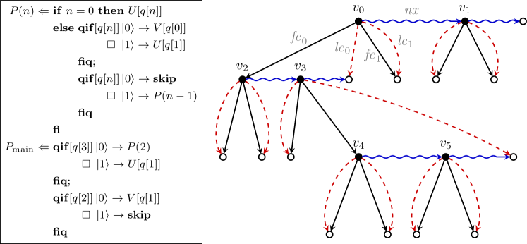
Figure 11: Example of a program in $\mathbf{RQC}^{++}$ and its corresponding qif table. In the qif table, we only show the links $\mathit{fc}_{i}$ (colored in black), $\mathit{lc}_{i}$ (colored in red and dashed) and $\mathit{nx}$ (colored in blue and squiggled), while $w$, $\mathit{cf}$, $\mathit{cl}$ and $\mathit{pr}$ are omitted for simplicity.

In Figure 11, we give an example of a program and its corresponding qif table. We only show the links $\mathit{fc}_{i}$, $\mathit{lc}_{i}$ and $\mathit{nx}$, and omit $\mathit{w}$, $\mathit{cf}$, $\mathit{cl}$ and $\mathit{pr}$ for simplicity of presentation. The partial evaluation should be done on the compiled program, but for clarity we present the original program written in $\mathbf{RQC}^{++}$. Let us explain the nodes in the qif table in Figure 11:

• $v_{0}$ represents the instantiation of the first $\mathbf{qif}\ldots\mathbf{fiq}$ in $P_{\textup{main}}$.

• $v_{1}$ represents the instantiation of the second $\mathbf{qif}\ldots\mathbf{fiq}$ in $P_{\textup{main}}$.

• $v_{2}$ and $v_{4}$ represent the first and second instantiations of the first $\mathbf{qif}\ldots\mathbf{fiq}$ in $P(n)$.

• $v_{3}$ and $v_{5}$ represent the first and second instantiations of the second $\mathbf{qif}\ldots\mathbf{fiq}$ in $P(n)$.

It is easy to verify that the links are consistent with Definition 2.

Additionally, we remark that to store the qif table in the QRAM, we need to encode all links and counter recorded at a node. The simplest way is to store them into a tuple, where links like $v.\mathit{nx}$ records the base address of the tuple of the corresponding node. Further discussion can be found in Section D.1. Another example of qif table for the quantum multiplexor program is provided in Section D.2.

5.2.2 Generation of Qif Table

For a compiled program $\mathcal{P}$, we fix a practical running time $T_{\textup{prac}}\left\lparen\mathcal{P}\right\rparen$. The partial evaluation is performed by multiple parallel processes. We classically emulate the execution of the compiled program, neglecting all quantum inputs and unitary gates. Whenever a qif is met, the current process forks into two sub-processes, each continuing the evaluation of the corresponding quantum branch. Whenever a fiq is met, the current process waits for its pairing sub-process, and collects information from both sub-processes to merge into one process. Every process only goes into a single quantum branch and therefore contains no quantum superposition.

For each process, we maintain the following classical information. We have $6$ system registers $\mathit{pc}$, $\mathit{ins}$, $\mathit{br}$, $\mathit{sp}$, $v$, $t$ and a constant number of user registers. Here, $v$ points to the current node in the qif table, and $t$ is a counter that records the number of instructions already executed. We also have a classical memory $M$ storing classical variables and the stack. Let $M_{i}$ be the value stored at the memory location $i$.

The algorithm for partial evaluation of quantum control flows and generation of the qif table is presented as Algorithm 1. The major part of the function QEva is the loop between Lines 3–16, which consists of three stages that also appear in the execution in Section 6. The first and the last stages are similar to their classical counterparts. We need to carefully explain the stage (Decode & Execute), in particular, when the current instruction is qif or fiq.

• If $\mathit{ins}=$ qif(q), then we meet a creation of quantum branching. We create two new nodes $v_{0},v_{1}$ and link them with the current node $v$. Then, the current process QEva is forked into two sub-processes QEva₀ and QEva₁, going into branches $q=0$ and $q=1$, respectively. For QEva_i, we update the current node $v$ by the children node $v_{i}$.

• If $\mathit{ins}=$ fiq(q), then we meet a join of quantum branching. We wait for the pairing sub-process QEva^′ with the same parent node $\hat{v}=v^{\prime}.\mathit{cl}=v.\mathit{cl}$. Given $\hat{t}=\max\left\{t,t^{\prime}\right\}$, we can calculate the number of instruction cycles to wait at the nodes $v$ and $v^{\prime}$. The wait counters $v.w,v^{\prime}.w$ will be used later in Section 6 to synchronise the two quantum branches (see also Section 5.1). After collecting the information in two quantum branches, we can merge the current process QEva with the pairing process QEva^′ into one by updating $t$ with $\hat{t}$ and $v$ with $\hat{v}$.

  Finally, we create a new node $u$ for the continuing quantum branch. We link $v$ and $u$ via $\mathit{nx}$ (and $\mathit{pr}$), and update $u$ as the new last children node for the parent node $\hat{u}$ of the current node $v$. Then, we update the current node $v$ by $u$.

Algorithm 1 returns a timeout error if $t$ exceeds the practical running time $T_{\textup{prac}}\left\lparen\mathcal{P}\right\rparen$. Otherwise, we obtain the actual running time $t=T_{\textup{exe}}\left\lparen\mathcal{P}\right\rparen$ for later use in Section 6. More detailed explanation of Algorithm 1 is deferred to Section D.3.

Algorithm 1 Partial evaluation of quantum control flow and generation of qif table.

QEva

1:Initialise $\mathit{pc}\leftarrow\text{starting address of the compiled main program}$ and $t\leftarrow 0$

2:Create an initial node $v$ $t\leq T_{\textup{prac}}\left\lparen\mathcal{P}\right\rparen$ [fill=blue!5!white]

3:(Fetch): Let $\mathit{ins}\leftarrow M_{\mathit{pc}}$ and $t\leftarrow t+1$ [fill=red!5!white]

4:(Decode & Execute): $\mathit{ins}=\texttt{qif(q)}$

5:Create nodes $v_{0}$ and $v_{1}$. Set $v.\mathit{fc}_{i},v.\mathit{lc}_{i}\leftarrow v_{i}$ and $v_{i}.\mathit{cf},v_{i}.\mathit{cl}\leftarrow v$

6:Fork into two sub-processes QEva₀ and QEva₁. For QEva_i, set $v\leftarrow v_{i}$ $\mathit{ins}=\texttt{fiq(q)}$

7:Wait for the pairing sub-process QEva^′ with $v^{\prime}.\mathit{cl}=v.\mathit{cl}=\hat{v}$ for some $\hat{v}$

8:$\hat{t}\leftarrow\max\{t,t^{\prime}\}$, $v.w\leftarrow\hat{t}-t$ and $v^{\prime}.w\leftarrow\hat{t}-t^{\prime}$ $\triangleright$ $v^{\prime},t^{\prime}$ are corresponding $v,t$ in QEva^′.

9:Merge with the pairing sub-process QEva^′ by letting $t\leftarrow\hat{t}$ and $v\leftarrow\hat{v}$

10:Create node $u$. Set $v.\mathit{nx}\leftarrow u$ and $u.\mathit{pr}\leftarrow v$. Suppose $v.\mathit{cl}=\hat{u}$ and $\hat{u}.\mathit{lc}_{x}=v$ for some $\hat{u}$ and $x$. Let $u.\mathit{cl}\leftarrow\hat{u}$, $\hat{u}.\mathit{lc}_{x}\leftarrow u$ and $v.\mathit{cl}\leftarrow 0$

11:Update $v\leftarrow u$ $\mathit{ins}=\texttt{finish}$

12:$t$ $\mathit{ins}\notin\{\texttt{uni(G,r)},\texttt{unib(G,r${}_{1}$,r${}_{2}$)}\}$

13:Update registers and $M$ according to Figure 5(a) [fill=green!5!white]

14:(Branch): $\mathit{br}\neq 0$

15:Let $\mathit{pc}\leftarrow\mathit{pc}+\mathit{br}$

16:Let $\mathit{pc}\leftarrow\mathit{pc}+1$

17:Timeout error

6 Execution on Quantum Register Machine

Now we are ready to describe how the compiled program $\mathcal{P}$ is executed, with the aid of partial evaluation results (including symbol table and qif table), on the quantum register machine. Let us load all these instructions and data into the QRAM, according to the layout described in Section 3.2.1.

6.1 Unitary $U_{\textup{cyc}}$ and Unitary $U_{\textup{exe}}$

Algorithm 2 presents the execution on quantum register machine, which consists of repeated cycles, each performing the unitary $U_{\textup{cyc}}$. We fix the number of repetitions to be $T_{\textup{exe}}=T_{\textup{exe}}\left\lparen\mathcal{P}\right\rparen$, obtained from Algorithm 1.

In $U_{\textup{cyc}}$, we need to decide whether to wait (i.e., skip the current cycle) or execute, according to the wait counter information stored in the current node of the qif table. To reversibly implement this procedure, $U_{\textup{cyc}}$ consists of the following three stages:

1. (Set wait flag): We check whether the value $w$ in the wait counter $\mathit{qifw}$ is $>0$. At this point, we are promised the wait flag $\mathit{wait}$ is in state $\ket{0}$. If $w>0$, then we flip $\mathit{wait}$ to $\ket{1}$.

2. (Execute or wait): Conditioned on the wait flag $\mathit{wait}$, we decide whether to wait or apply $U_{\textup{exe}}$ (defined in Algorithm 2 and explained later). If the wait flag is $\ket{0}$, then we apply $U_{\textup{exe}}$; if the wait flag is $\ket{1}$, then we decrement the wait counter $w$ in register $\mathit{qifw}$ by $1$.

3. (Clear wait flag): We clear the wait flag $\mathit{wait}$, according to the value $w$ in $\mathit{qifw}$ and the counter information $v.w$, where $v$ is the value in $\mathit{qifv}$. Specially, if $w<v.w$, then the wait flag is set previously and needs to be cleared now. Note that $v.w$ is stored in the qif table, and needs to be fetched into some free register by $U_{\textup{fet}}$ before being used, of which details are omitted for simplicity. After this stage, $\mathit{wait}$ is guaranteed to be in state $\ket{0}$.

As a subroutine of $U_{\textup{cyc}}$, the unitary $U_{\textup{exe}}$ consists of four stages. They are inspired by the design of classical reversible processor (e.g., [68]) and need little explanation. In the (Decode & Execute) stage, the unitary $U_{\textup{dec}}$ is defined in Figure 5(b). We provide more detailed discussion on Algorithm 2 and its visualisation as quantum circuits in Section E.1.

Algorithm 2 Execution on quantum register machine.

$U_{\textup{main}}$

1:Initialise registers according to Section 3.1 $t=1,\ldots,T_{\textup{exe}}$

2:Apply the unitary [fill=blue!5!white]$U_{\textup{cyc}}$ (defined below) [fill=blue!5!white] $U_{\textup{cyc}}$

3:(Set wait flag): Conditioned on $\mathit{qifw}$, set the wait flag in $\mathit{wait}$:

4:    Perform $\sum_{w,z}\ket{w}\!\bra{w}_{\mathit{qifw}}\otimes\ket{z\oplus\left[w>0\right]}\!\bra{z}_{\mathit{wait}}$

5:(Execute or wait): Conditioned on $\mathit{wait}$, apply the unitary [fill=red!5!white]$U_{\textup{exe}}$ (defined below), or wait and decrement the value in $\mathit{qifw}$:

6:    Perform $\ket{0}\!\bra{0}_{\mathit{wait}}\otimes U_{\textup{exe}}+\sum_{z\neq 0,w}\ket{z}\!\bra{z}_{\mathit{wait}}\otimes\ket{w-1}\!\bra{w}_{\mathit{qifw}}\otimes\mathbbm{1}$

7:(Clear wait flag): Conditioned $\mathit{qifw}$ and $\mathit{qifv}$, uncompute the wait flag in $\mathit{wait}$:

8:    Perform $\sum_{w,v,z}\ket{w}\!\bra{w}_{\mathit{qifw}}\otimes\ket{v}\!\bra{v}_{\mathit{qifv}}\ket{z\oplus\left[w<v.w\right]}\!\bra{z}_{\mathit{wait}}$ [fill=red!5!white] $U_{\textup{exe}}$

9:(Fetch): Apply the unitary $U_{\textup{fet}}\left\lparen\mathit{ins},\mathit{pc},\mathit{mem}\right\rparen$ $\triangleright$ $U_{\textup{fet}}$ is defined in Definition 1.

10:(Decode & Execute): Apply the unitary $U_{\textup{dec}}$ $\triangleright$ $U_{\textup{dec}}$ is defined in Figure 5(b).

11:(Unfetch): Apply the unitary $U_{\textup{fet}}\left\lparen\mathit{ins},\mathit{pc},\mathit{mem}\right\rparen$ again

12:(Branch): Update $\mathit{pc}$, conditioned on $\mathit{br}$:

13:    Apply $U_{+}\left\lparen\mathit{pc},\mathit{br}\right\rparen$ $\triangleright$ $U_{+}$ performs the mapping $\ket{x}\ket{y}\mapsto\ket{x+y}\ket{y}$.

14:    Apply $\circ\left\lparen\mathit{br}\right\rparen$-$\sum_{x}\ket{x+1}\!\bra{x}_{\mathit{pc}}$ $\triangleright$ $\circ\left\lparen\cdot\right\rparen$-$U$ is defined in Section 3.3.

6.2 Unitaries for Executing Qif Instructions

It remains to define the unitaries $U_{\textup{qif}}$ and $U_{\textup{fiq}}$ that are unspecified in Figure 5(a). We present their constructions in Algorithm 3. Additional remarks are as follows.

• For $U_{\textup{qif}}$, note that we are promised that $\mathit{qifw}$ is initially in state $\ket{0}$, because $U_{\textup{qif}}$ is used as a subroutine in $U_{\textup{exe}}$, which will only be called by $U_{\textup{cyc}}$ when the wait counter $\mathit{qifw}$ is in state $\ket{0}$.

• As aforementioned, the information $\mathit{fc}_{x}$, $\mathit{cf}$, $\mathit{lc}_{x}$, $\mathit{cl}$, $\mathit{nx}$, $\mathit{pr}$ and $w$ are stored in the qif node, and need to be fetched using $U_{\textup{fet}}$ into free registers before being used, of which details are omitted for simplicity.

Further explanation of Algorithm 3 is provided in Section E.2.

Algorithm 3 The unitaries $U_{\mathit{qif}}$ and $U_{\mathit{fiq}}$ in Figure 5(b).

$U_{\textup{qif}}$$q$

1:Conditioned on $q$, move $\mathit{qifv}$ to its first children node in the qif table via the links $\mathit{fc}_{0}$ and $\mathit{fc}_{1}$; i.e., perform the following series of unitaries:

2:    $V_{\mathit{fc}}=\sum_{v,x,u}\ket{v}\!\bra{v}_{\mathit{qifv}}\otimes\ket{x}\!\bra{x}_{q}\otimes\ket{u\oplus v.\mathit{fc}_{x}}\!\bra{u}_{r}$, where $r$ is a free register

3:    $V_{\mathit{cf}}=\sum_{v,u}\ket{v\oplus u.\mathit{cf}}\!\bra{v}_{\mathit{qifv}}\otimes\ket{u}\!\bra{u}_{r}$

4:    $U_{\textup{swap}}\left\lparen r,\mathit{qifv}\right\rparen$, which also clears register $r$ $\triangleright$ $U_{\textup{swap}}$ is defined in Section 3.3.

5:Update $\mathit{qifw}$ with the wait counter information corresponding to $\mathit{qifv}$; i.e., perform:

6:    $\sum_{w,v}\ket{v}\!\bra{v}_{\mathit{qifv}}\otimes\ket{w\oplus v.w}\!\bra{w}_{\mathit{qifw}}$ $U_{\textup{fiq}}$$q$

7:Conditioned on $q$, move $\mathit{qifv}$ to its parent node in the qif table via the inverse link $\mathit{cl}$; i.e., perform the following series of unitaries:

8:    $V_{\mathit{cl}}=\sum_{v,u}\ket{v}\!\bra{v}_{\mathit{qifv}}\otimes\ket{u\oplus v.\mathit{cl}}\!\bra{u}_{r}$, where $r$ is a free register

9:    $V_{\mathit{lc}}=\sum_{v,x,u}\ket{v\oplus u.\mathit{lc}_{q}}\!\bra{v}_{\mathit{qifv}}\otimes\ket{x}\!\bra{x}_{q}\otimes\ket{u}\!\bra{u}_{r}$

10:    $U_{\textup{swap}}\left\lparen r,\mathit{qifv}\right\rparen$, which also clears register $r$

11:Move $\mathit{qifv}$ to the next node in the qif table via the link $\mathit{nx}$; i.e., perform the following series of unitaries:

12:    $V_{\mathit{nx}}=\sum_{v,u}\ket{v}\!\bra{v}_{\mathit{qifv}}\otimes\ket{u\oplus v.\mathit{nx}}\!\bra{u}_{r}$, where $r$ is a free register

13:    $V_{\mathit{pr}}=\sum_{v,u}\ket{v\oplus u.\mathit{pr}}\!\bra{v}_{\mathit{qifv}}\otimes\ket{u}\!\bra{u}_{r}$

14:    $U_{\textup{swap}}\left\lparen r,\mathit{qifv}\right\rparen$, which also clears register $r$

Now we remark on how the qif table as a classical data structure is used in quantum superposition during the execution on quantum register machine. Recall that at runtime, the value in register $\mathit{qifv}$ indicates the current node in the qif table. Register $\mathit{qifv}$ can be in a quantum superposition state, in particular, entangled with the quantum coin $q$ (as well as other register and the QRAM) when instruction qif(q) is executed (see Algorithm 3). For example, after the unitary $U_{\textup{qif}}(q)$ is performed, the state of the quantum register machine can be $\frac{1}{\sqrt{2}}\ket{0}_{q}\ket{v_{1}}_{\mathit{qifv}}\ket{\psi_{0}}+\frac{1}{\sqrt{2}}\ket{1}_{q}\ket{v_{2}}_{\mathit{qifv}}\ket{\psi_{1}}$, where $\ket{\psi_{0}}$ and $\ket{\psi_{1}}$ are states of the remaining quantum registers and the QRAM. In this way, the information in the qif table is used in quantum superposition.

7 Efficiency and Automatic Parallelisation

An implementation of quantum recursive programs has been presented in the previous sections. In this section, we analyse its efficiency, and further show that as a bonus, such implementation also offers automatic parallelisation. For implementing certain algorithmic subroutine, like the quantum multiplexor introduced in Section 1.1, we can even obtain exponential parallel speed-up (over the straightforward implementation) from this automatic parallelisation. This steps towards a top-down design of efficient quantum algorithms: we only need to design high-level quantum recursive programs, and let the machine automatically realise the parallelisation (whose quality, of course, still depends on the structures in the programs). The intuition for the automatic parallelisation was already pointed out in Section 1.1: with quantum control flows, the quantum register machine can go through quantum branches in superposition; and with recursive procedure calls, the program can generate exponentially many quantum branches (as each instantiation of the $\mathbf{qif}$ statement creates two quantum branches).

In the following, we briefly analyse the complexity of implementing quantum recursive programs; in particular, the costs for the partial evaluation and execution. More details can be found in Sections D.4 and E.3.

1. Algorithm 1 takes $O\left\lparen T_{\textup{exe}}\left\lparen\mathcal{P}\right\rparen\right\rparen$ classical parallel elementary operations. The adjective “elementary” means the operation only involves a constant number of memory locations in the classical RAM (as the partial evaluation is performed classically). The adjective “parallel” means multiple elementary operations performed simultaneously are counted as one parallel elementary operation, like in the standard parallel computing.

   To see this, note that Algorithm 1 terminates correctly iff $t=T_{\textup{exe}}\left\lparen\mathcal{P}\right\rparen$. It suffices to show every step in QEva takes $O\left\lparen 1\right\rparen$ classical parallel elementary operations. When a process is forked into two sub-processes (e.g., Line 6), we need to create a copy of all data of the current process, which can be done using $O\left\lparen 1\right\rparen$ classical parallel elementary operations. The merging of sub-processes is similar. Other steps are rather simple. The full analysis is deferred to Section D.4.

2. Algorithm 2 takes $O\left\lparen T_{\textup{exe}}\left\lparen\mathcal{P}\right\rparen\right\rparen$ quantum elementary operations, including on registers and QRAM accesses (see Definition 1).

   To see this, note that the time complexity of $U_{\textup{main}}$ is dominated by that of the repeated applications of $U_{\textup{cyc}}$, while the latter is further dominated by that of $U_{\textup{exe}}$. It suffices to show that $U_{\textup{exe}}$ takes $O\left\lparen 1\right\rparen$ quantum elementary operations. The most expensive stage in $U_{\textup{exe}}$ is (Decode & Execute), where the unitary $U_{\textup{dec}}$ (see definition in Figure 5(b)) is applied. $U_{\textup{dec}}=\sum_{c}\ket{c}\!\bra{c}\otimes\sum_{d}\ket{d}\!\bra{d}\otimes U_{c,d}$ is essentially a quantum multiplexor, where the number of terms in the summation is $O\left\lparen 1\right\rparen$. So this reduces to verifying each $U_{c,d}$ takes $O\left\lparen 1\right\rparen$ quantum elementary operations, which is rather simple. The full analysis is deferred to Section E.3.

The above costs are given in terms of elementary operations. If we consider more refined time complexity, then the overall (classical and quantum) parallel time complexity of Algorithms 1 and 2 will be

$$O\left\lparen T_{\textup{exe}}\left\lparen\mathcal{P}\right\rparen\cdot\left\lparen T_{\textup{reg}}+T_{\textup{QRAM}}\right\rparen\right\rparen,$$

where $T_{\textup{reg}}$ and $T_{\textup{QRAM}}$ are parallel time complexities for elementary operations on registers and QRAM accesses, as aforementioned. Here, we assume that classical elementary operations are cheaper than their quantum counterparts.

For concreteness, let us return to the example of quantum multiplexor program $\mathcal{P}$ in Figure 1. Recall that in Figure 8 the programs after high-level transformations and high-to-mid-level translation are already presented, while the full compiled program is lengthy and deferred to Figure 18. Now we provide a proof sketch of Theorem 1, whose full proof is deferred to Section F.2.

Proof Sketch of Theorem 1.

Since each $C_{x}$ only consists of $T_{x}$ quantum unitary gates, the number of instructions in the compiled program of $P[x]\Leftarrow C_{x}$ will be $O\left\lparen T_{x}\right\rparen$. As a result, the whole compiled quantum multiplexor program (deferred to Figure 18) contains $\Theta\left\lparen\sum_{x\in[N]}T_{x}\right\rparen$ instructions. It is easy to verify that $T_{\textup{exe}}\left\lparen\mathcal{P}\right\rparen=O\left\lparen\max_{x\in[N]}T_{x}+n\right\rparen$.

Let us determine $T_{\textup{reg}}$ and $T_{\textup{QRAM}}$ by implementing the quantum register machine in the more common quantum circuit model. We can calculate the size $N_{\textup{QRAM}}$ of the QRAM and the word length $L_{\textup{word}}$ for implementing $\mathcal{P}$. In particular, taking $N_{\textup{QRAM}}=\Theta\left\lparen\sum_{x}T_{x}\right\rparen$ is sufficient. To see this, we can calculate that the sizes of the program, symbol table and variable sections are upper bounded by $\Theta\left\lparen\sum_{x}T_{x}\right\rparen$. The size of the qif table is $\Theta\left\lparen 2^{n}\right\rparen$. The size of the stack is upper bounded by $\Theta\left\lparen\sum_{x}T_{x}\right\rparen+\Theta\left\lparen n\right\rparen$. To store an address in such QRAM, taking $L_{\textup{word}}=\Theta\left\lparen\log N_{\textup{QRAM}}\right\rparen$ is sufficient.

By lifting results from classical parallel circuits for elementary arithmetic [52, 59, 9], we have $T_{\textup{reg}}=O\left\lparen\log^{2}L_{\textup{word}}\right\rparen$. By extending existing circuit QRAM constructions (e.g., [31, 34]), we have $T_{\textup{QRAM}}=O\left\lparen\log N_{\textup{QRAM}}+\log L_{\textup{word}}\right\rparen$. The above calculations are carried out in terms of parallel time complexity, i.e., quantum circuit depth. Combining the above arguments leads to Theorem 1. ∎

8 Related Work

Low-level quantum instructions

Several quantum instruction set architectures have been proposed in the literature, e.g., OpenQASM [21], Quil [64], eQASM [29]. Only the architecture introduced in [80], called quantum control machine, supports program counter in superposition (and hence quantum control flows), and the others do not support quantum control flows at the instruction level. Quantum control machine also supports conditional jumps, but different from quantum register machine defined in this paper, it does not support arbitrary procedure calls.

Automatic parallelisation

Numerous efforts have been devoted to parallelisation of quantum circuits of specific patterns, e.g., [20, 50, 32, 67, 37, 11, 66, 39, 84, 85, 60, 65, 82, 81]. Other than the quantum circuit model, the measurement-based quantum computing [58] is also shown to provide certain benefits for parallelisation [40, 23, 16, 17, 57, 22]. These techniques of parallelisation are at the low level. In comparison, the automatic parallelisation from our implementation is at the high level: the quantum register machine automatically exploits parallelisation opportunities in the structures of the high-level quantum recursive programs.

Automatic uncomputation

Silq [15] is the first quantum programming language that supports automatic uncomputation, which was further investigated in [55, 79, 71, 78, 56, 69]. Silq’s uncomputation is for quantum programs lifted from classical ones, or in their terminology, lifted functions (whose semantics can be described classically and preserves the input). Later works like [71, 69] also considered uncomputation of quantum programs but they do not support quantum recursion. In comparison, $\mathbf{RQC}^{++}$ supports quantum recursion, where classical variables are used solely for specifying the control (not data). The automatic uncomputation in our implementation is of these classical variables in quantum recursive programs.

Classical reversible languages

There are extensive works in classical reversible programming languages, including the high-level language Janus [48, 77, 76], low-level instruction set architectures PISA [70, 28, 5] and BobISA [68]. Some of these reversible languages support local variables, specified by a pair of local-delocal statements, which have explicitly reversible semantics. In $\mathbf{RQC}^{++}$, irreversible classical computation can be done on local variables, but their translations into low-level instructions become reversible.

9 Conclusion

We propose the notion of quantum register machine, an architecture that supports quantum control flows and recursive procedure calls at the same time. We design a comprehensive process of implementing quantum recursive programs on the quantum register machine, including compilation, partial evaluation of quantum control flows and execution. As a bonus, our implementation offers automatic parallelisation, from which we can even obtain exponential parallel speed-up (over the straightforward implementation) for implementing some important quantum algorithmic subroutines like the quantum multiplexor.

To conclude this paper, let us list several topics for future research. Firstly, an immediate next step is to develop a software that realises our implementation of quantum recursive programs for actual execution on future quantum hardware. Secondly, our implementation is designed to be simple for clarity. It is worth extending the features of the quantum register machine and further optimise the steps in the compilation, partial evaluation and execution. Thirdly, it is interesting to see what other quantum algorithms (except those considered in [75] and this paper) can be written in quantum recursive programs and benefit (with possible speed-up) from the efficient implementation of the quantum register machine.

Appendix A Quantum Recursive Programming Language $\mathbf{RQC}^{++}$

In this appendix, we provide a more detailed introduction to the syntax and semantics of high-level language $\mathbf{RQC}^{++}$ for describing quantum recursive programs [75]. For the purpose of this paper, we also make some slight modifications and more illustrations, compared to the original definitions of $\mathbf{RQC}^{++}$ in [75].

Let us first describe several features of the language $\mathbf{RQC}^{++}$. As aforementioned, it allows both quantum control flows and recursive procedure calls, and therefore supports the quantum recursion. For simplicity, $\mathbf{RQC}^{++}$ is not explicitly typed. A program in $\mathbf{RQC}^{++}$ describes a quantum circuit without measurements, whose size is parameterised. The alphabet of $\mathbf{RQC}^{++}$ contains classical and quantum variables, while classical variables solely serve for specifying the control of the programs. The quantum control flows in $\mathbf{RQC}^{++}$ are fully managed by the $\mathbf{qif}$ statements: quantum branches are only created by $\mathbf{qif}$, and only merged by $\mathbf{fiq}$.

A.1 Program Variables and Procedure Identifiers

A.1.1 Classical Variables

Classical variables in $\mathbf{RQC}^{++}$ are solely for specifying the control of programs. A program in $\mathbf{RQC}^{++}$ describes a quantum unitary transformation, whose dimension can depend on classical parameters. Classical variables are classical only in the eyes of the programmer; or more specifically, in the eyes of the enclosing procedure. Meanwhile, the procedure calls can be used in quantum superposition, e.g., within quantum branches created by the $\mathbf{qif}$ statements. In the implementation, classical variables will be realised by the quantum hardware instead.

A classical variable $x$ has a type $T(x)$, which can be thought of as a set; i.e., $x\in T\left\lparen x\right\rparen$. In this paper, we will only consider three types of classical variables, $\mathbf{Uint}$, $\mathbf{Int}$ and $\mathbf{Bit}$, standing for unsigned integer type, integer type and bit type, respectively. We use $\overline{x}=x_{1}x_{2}\ldots x_{n}$ to denote a list of classical variables.

A.1.2 Quantum Variables

Quantum variables are very different from classical variables. The state of quantum variables can be in superposition, and different quantum variables can be entangled. An elementary quantum variable $q$ has a type $T(q)=\mathcal{H}$, which represents the corresponding Hilbert space of $q$. The type (Hilbert space) of a list $\overline{q}$ of distinct quantum variables $q_{1},\ldots,q_{n}$ is then the tensor product $T(\overline{q})=\bigotimes_{i=1}^{n}\mathcal{H}_{i}$, where each $\mathcal{H}_{i}=T(q_{i})$ is the type of $q_{i}$. In this paper, we will only consider two types of quantum variables, $\mathbf{Qint}$ and $\mathbf{Qbit}$, standing for quantum integer type and qubit type, respectively.

A.1.3 Procedure Identifiers

Procedure identifiers are the names of procedures and are of a designated type $\mathbf{Pid}$. For each procedure identifier $P$, we can correspond to it a classical variable $P.\mathit{ent}$ of type $\mathbf{Uint}$, storing the entry address of the procedure declaration of $P$. The value of $P.\mathit{ent}$ is determined and static after the program is compiled and loaded into the memory. In the compiled program, $P.\mathit{ent}$ will be used for handling procedure calls (see also Section 4.3).

A.1.4 Arrays

Classical and quantum variables can all be generalised to array variables. Procedure identifiers can be generalised to procedure arrays too. An array can be subscripted by classical values. For simplicity of presentation, in this paper, we only consider one-dimensional arrays. High-dimensional arrays can be easily simulated by one-dimensional arrays.

The type of an array depends on the type of its elements:

1. The type of a classical array $x$ is $\left\lparen T\rightarrow X\right\rparen\equiv X^{T}$, where $X$ is the type of the elements in $x$, and $T$ is the type of the subscript.

2. The type of a quantum array $q$ is $\left\lparen T\rightarrow\mathcal{H}\right\rparen\equiv\bigotimes_{t\in T}\mathcal{H}_{t}$, where $\mathcal{H}_{t}=\mathcal{H}$ is the type of the element, and $T$ is the type of the subscript.

3. The type of a procedure array is $\left\lparen T\rightarrow\mathbf{Pid}\right\rparen\equiv\mathbf{Pid}^{T}$, where $T$ is the type of the subscript.

Elements in a classical or quantum array are assigned contiguous addresses in the memory (see also Section C.3), and hence can be efficiently addressed.

Given an array variable, we can also write corresponding subscripted variables. For classical array $x$ of type $T\rightarrow X$ and quantum array $q$ of type $T\rightarrow\mathcal{H}$, we can write subscripted variables $x[t]$, $q[t]$ for classical expression $t$ of type $T$, respectively. They are of types $X$ and $\mathcal{H}$, respectively. For example, one can write subscripted quantum variable $q[5x+2y]$, where $x,y$ are classical variables. Similarly, given a procedure array $P$, we can also write corresponding subscripted procedure identifiers $P[t]$.

For simplicity of presentation, we restrict the use of nested subscriptions. In particular, for classical subscripted variable $x[t]$, we require that $t$ contains no more subscripted variables. For example, we do not allow subscripted variable $x[y[10]]$ for classical $x,y$, but allow $q[x[7z]]$ for quantum $q$ and classical $x,z$. The implementation of nested subscriptions can actually be treated in similar but more complicated ways.

Suppose $x$ is a classical array of type $T\rightarrow X$ with $T=\mathbf{Uint}$ or $\mathbf{Int}$. We use the notation $x[k:l]$ to denote the restriction of $x$ to the interval $[k:l]=\left\{k,k+1,\ldots,l-1,l\right\}$. Then, $x[k:l]$ is a variable of type $[k:l]\rightarrow X$. The same convention applies to quantum and procedure arrays.

A.1.5 Global Variables vs. Local Variables

In $\mathbf{RQC}^{++}$, a variable is not declared before its use. All variables are treated as global variables. Local (classical) variables will be realised by the block statement

$$\mathbf{begin}\ \mathbf{local}\ \overline{x}:=\overline{t};\ldots\mathbf{end}.$$

Within the scope of the block, the list of classical variables $\overline{x}$ are regarded as local variables, initialised to new values specified by the list of expressions $\overline{t}$ at the begining of the block, and restore their old values at the end of the block. A consequence of this treatment is that in a procedure call, the callee can use the variables setting up by the caller.

A.2 Syntax

The syntax of $\mathbf{RQC}^{++}$ is already summarised in Figure 2. Here, we provide some more detailed explanations.

A.2.1 Classical Assignment, If-Statement and Loop

In $\mathbf{RQC}^{++}$, the classical assignment, if-statement and loop are similar to their counterparts in classical programming languages.

• The assignment $\overline{x}:=\overline{t}$ simultaneously assigns the values of the list of expressions $\overline{t}$ to the list of classical variables $\overline{x}$. Note that in $\overline{t}=t_{1}t_{2}\ldots t_{n}$, $t_{i}$ might contains variables in $\overline{x}=x_{1}x_{2}\ldots x_{n}$.

• The $\mathbf{if}\ b\ \mathbf{then}\ C_{1}\ \mathbf{else}\ C_{2}\ \mathbf{fi}$ statement chooses one of statements $C_{1}$ and $C_{2}$ to execute, depending on the value of the boolean expression $b$.

• The $\mathbf{while}\ b\ \mathbf{do}\ C\ \mathbf{od}$ statement repeatedly execute statement $C$, conditioned on that the value of the boolean expression $b$ is $1$.

A.2.2 Block Statement

The block statement is used to declare classical variables as local variables. In particular, the statement

$$\mathbf{begin}\ \mathbf{local}\ \overline{x}:=\overline{t};\ C\ \mathbf{end}$$

declares the list of variables $\overline{x}$ as local variables within the scope of $\mathbf{begin}\ldots\mathbf{end}$, initialised to values of the list of expressions $\overline{t}$. At the end of the block, $\overline{x}$ will restore the old values. The block statement is also useful in defining the semantics of procedure calls (see Section A.3).

A.2.3 Procedure Call

The procedure call and procedure declaration are also similar to their classical counterparts.

• The procedure declaration $P\left\lparen\overline{u}\right\rparen\Leftarrow C$ declares a procedure identifier $P$ with the list of formal parameters $\overline{u}$ and procedure body $C$.

• The procedure call $P\left\lparen\overline{t}\right\rparen$ calls the procedure with identifier $P$ with the list of actual parameter $\overline{t}$.

A.2.4 Quantum Unitary Gate

The statement $U[\overline{q}]$ applies an elementary quantum unitary gate $U$ on the list $\overline{q}$ of quantum variables. For simplicity of presentation, we restrict that $\overline{q}$ contains at most two quantum variables, which are of type $\mathbf{Qbit}$. The type of the unitary gate $U$ needs to be matched with $\overline{q}$. If $\overline{q}=q_{1}$, then $U$ is a single-qubit unitary gate; if $\overline{q}=q_{1}q_{2}$, then $U$ is a two-qubit unitary gate. Moreover, we restrict that $U$ is chosen from a fixed set of elementary unitary gate set $\mathcal{G}$ of size $\left\lvert\mathcal{G}\right\rvert=O(1)$. For example, $\mathcal{G}=\left\{H,T,\mathit{CNOT}\right\}$. More complicated unitaries, like parameterised rotation $R_{X}(\theta)$, can be implemented by procedure call with classical parameters.

A.2.5 Quantum Control Flow

The quantum if-statement $\mathbf{qif}[q]\left\lparen\ket{0}\rightarrow C_{0}\right\rparen\square\left\lparen\ket{1}\rightarrow C_{1}\right\rparen\mathbf{fiq}$ in $\mathbf{RQC}^{++}$ explicitly manages quantum control flows. Unlike the classical if-statement with classical control flow, the control flow in the $\mathbf{qif}$ statement is essentially quantum. Conditioned on the value ($\ket{0}$ or $\ket{1}$) of the external quantum coin $q$, the statements $C_{0}$ and $C_{1}$ will be executed. When $q$ is in a quantum superposition state, the subsystems that $C_{0}$ and $C_{1}$ act on will be entangled with $q$. The condition of the external quantum coin is to promise the physicality of the $\mathbf{qif}$ statement, which is already stated in Condition 1, and will be further explained later when we come to the semantics of $\mathbf{RQC}^{++}$.

It is also worth pointing out that in $\mathbf{RQC}^{++}$, the quantum control flows are fully guarded by the $\mathbf{qif}$ statements. In particular, quantum branches are only created by $\mathbf{qif}$, and only merged by $\mathbf{fiq}$.

A.3 Semantics

As aforementioned in Section 2.2, the operational semantics of $\mathbf{RQC}^{++}$ is defined in terms of transitions between configurations. A configuration is represented by $\left\lparen C,\sigma,\ket{\psi}\right\rparen$, where $C$ is the remaining statement to be executed or $C=\ \downarrow$ (standing for termination; and we denote $\downarrow;C^{\prime}\equiv C^{\prime}$), $\sigma$ is the current classical state of all classical variables, and $\ket{\psi}$ is the current quantum state of all quantum variables. Let $\mathcal{C}$ be the set of configurations. Then, the operational semantics is defined as the transition relation $\rightarrow\ \in\mathcal{C}\times\mathcal{C}$, of the form $\left\lparen C,\sigma,\ket{\psi}\right\rparen\rightarrow\left\lparen C^{\prime},\sigma^{\prime},\ket{\psi^{\prime}}\right\rparen$, by a series of transition rules. Due to the limited space there, we only gave the transition rule for quantum if-statement in Figure 3. Now we present all transition rules for defining the operational semantics of $\mathbf{RQC}^{++}$ in Figure 12. Let us also further explain some of them as follows.

$$(\textup{SK}) \ \left\lparen\mathbf{skip},\sigma,\ket{\psi}\right\rparen\rightarrow\left\lparen\downarrow,\sigma,\ket{\psi}\right\rparen$$

$$(\textup{AS}) \ \left\lparen\overline{x}:=\overline{t},\sigma,\ket{\psi}\right\rparen\rightarrow\left\lparen\downarrow,\sigma\left[\overline{x}:=\sigma\left\lparen\overline{t}\right\rparen\right],\ket{\psi}\right\rparen$$

$$(\textup{GA}) \ \left\lparen U\left[\overline{q}\right],\sigma,\ket{\psi}\right\rparen\rightarrow\left\lparen\downarrow,\sigma,\left\lparen U_{q}\otimes\mathbbm{1}\right\rparen\ket{\psi}\right\rparen$$

$$(\textup{SC}) \ \frac{\left\lparen C_{1},\sigma,\ket{\psi}\right\rparen\rightarrow\left\lparen C_{1}^{\prime},\sigma^{\prime},\ket{\psi^{\prime}}\right\rparen}{\left\lparen C_{1};C_{2},\sigma,\ket{\psi}\right\rparen\rightarrow\left\lparen C_{1}^{\prime};C_{2},\sigma^{\prime},\ket{\psi^{\prime}}\right\rparen}$$

$$(\textup{IF}) \ \frac{\sigma\models b}{\left\lparen\mathbf{if}\ b\ \mathbf{then}\ C_{1}\ \mathbf{else}\ C_{2}\ \mathbf{fi},\sigma,\ket{\psi}\right\rparen\rightarrow\left\lparen C_{1},\sigma,\ket{\psi}\right\rparen}$$

$$\ \frac{\sigma\models\neg b}{\left\lparen\mathbf{if}\ b\ \mathbf{then}\ C_{1}\ \mathbf{else}\ C_{2}\ \mathbf{fi},\sigma,\ket{\psi}\right\rparen\rightarrow\left\lparen C_{2},\sigma,\ket{\psi}\right\rparen}$$

$$(\textup{LP}) \ \frac{\sigma\models b}{\left\lparen\mathbf{while}\ b\ \mathbf{do}\ C\ \mathbf{od},\sigma,\ket{\psi}\right\rparen\rightarrow\left\lparen C;\mathbf{while}\ b\ \mathbf{do}\ C\ \mathbf{od},\sigma,\ket{\psi}\right\rparen}$$

$$\ \frac{\sigma\models\neg b}{\left\lparen\mathbf{while}\ b\ \mathbf{do}\ C\ \mathbf{od}\right\rparen,\sigma,\ket{\psi}\rightarrow\left\lparen\downarrow,\sigma,\ket{\psi}\right\rparen}$$

$$(\textup{QIF}) \ \frac{\ket{\psi}=\alpha_{0}\ket{0}_{q}\ket{\theta_{0}}+\alpha_{1}\ket{1}_{q}\ket{\theta_{1}},\qquad\left\lparen C_{i},\sigma,\ket{\theta_{i}}\right\rparen\rightarrow^{*}\left\lparen\downarrow,\sigma^{\prime},\ket{\theta_{i}^{\prime}}\right\rparen\ (i=0,1)}{\left\lparen\mathbf{qif}\left[q\right]\left\lparen\ket{0}\rightarrow C_{0}\right\rparen\square\left\lparen\ket{1}\rightarrow C_{1}\right\rparen\mathbf{fiq},\sigma,\ket{\psi}\right\rparen\rightarrow\left\lparen\downarrow,\sigma^{\prime},\alpha_{0}\ket{0}_{q}\ket{\theta_{0}^{\prime}}+\alpha_{1}\ket{1}_{q}\ket{\theta_{1}^{\prime}}\right\rparen}$$

$$(\textup{BS}) \ \left\lparen\mathbf{begin}\ \mathbf{local}\ \overline{x}:=\overline{t};C\ \mathbf{end},\sigma,\ket{\psi}\right\rparen\rightarrow\left\lparen\overline{x}:=\overline{t};C;\overline{x}:=\sigma\left\lparen\overline{x}\right\rparen,\sigma,\ket{\psi}\right\rparen$$

$$(\textup{RC}) \ \frac{P\left\lparen\overline{u}\right\rparen\Leftarrow C\in\mathcal{P}}{\left\lparen P\left\lparen\overline{t}\right\rparen,\sigma,\ket{\psi}\right\rparen\rightarrow\left\lparen\mathbf{begin}\ \mathbf{local}\ \overline{u}:=\overline{t};C\ \mathbf{end},\sigma,\ket{\psi}\right\rparen}$$

Figure 12: Transition rules for defining the operational semantics of $\mathbf{RQC}^{++}$.

• In the (QIF) rule, we see how the condition of external quantum coin (Condition 1, in which $\mathit{qv}$ will be defined in Definition 3 below) is used: it promises that $q$ is separated from the subsystems that $C_{0}$ and $C_{1}$ act on, and therefore the current state $\ket{\psi}$ can be written as $\alpha_{0}\ket{0}_{q}\ket{\theta_{0}}+\alpha_{1}\ket{1}_{q}\ket{\theta_{1}}$.

  Another point to note is that the executions of $C_{i}$ in both quantum branches ($i=0,1$) take the same classical state $\sigma$ to the same $\sigma^{\prime}$. This promises that classical variables are disentangled from quantum variables after the $\mathbf{qif}$ statement, and thus $\sigma^{\prime}$ will not be in superposition. It is worth pointing out that classical variables in $\mathbf{RQC}^{++}$ are classical only in the eyes of the programmer (or the enclosing procedure); they become quantum when the program is implemented on quantum hardware.

• In the (BS) rule, the sequential composition $\overline{x}:=\overline{t};C;\overline{x}:=\sigma\left\lparen\overline{x}\right\rparen$ formalises the meaning of initialising $\overline{x}$ at the beginning of the block and restoring their old values (i.e., $\sigma\left\lparen\overline{x}\right\rparen$) at the end of the block.

• In the (RC) rule, the formal parameters $\overline{u}$ to be used by the callee will be locally replaced by the actual parameters $\overline{t}$ set by the caller.

A.3.1 Conditions for Well-defined Semantics

A program written in the syntax in Figure 2 is not yet promised to have well-defined semantics. To guarantee that a program in $\mathbf{RQC}^{++}$ has well-defined semantics, recall that in Section 2.3 we introduce three conditions (Conditions 1, 2 and 3), in which two notions are remained to be formally defined.

The first notion is the quantum variables $\mathit{qv}\left\lparen C,\sigma\right\rparen$ in a statement $C$ with respect to a given classical state $\sigma$. It is used in Condition 1. Before formally defining $\mathit{qv}$, we need some additional notions. We use $\mathcal{Q}\mathcal{V}$ to denote the set of all quantum variables. Let $\mathcal{C}^{\prime}$ be the set of classical configurations of the form $(C,\sigma)$. Let $\mathcal{F}\equiv\mathcal{C}^{\prime}\rightarrow 2^{\mathcal{Q}\mathcal{V}}$ be the set of functions $f$ that maps a configuration $(C,\sigma)\in\mathcal{C}^{\prime}$ to a set of quantum variables $f(C,\sigma)\in 2^{\mathcal{Q}\mathcal{V}}$. Then, we can define a partial order $\sqsubseteq$ on $\mathcal{F}$, such that for $f,g\in\mathcal{F}$, $f\sqsubseteq g$ iff $\forall(C,\sigma)\in\mathcal{C}^{\prime}$, $f(C,\sigma)\subseteq g(C,\sigma)$.

Definition 3 (Quantum variables).

For a statement $C\in\mathbf{RQC}^{++}$ and a classical state $\sigma$, the quantum variables of $C$ with respect to $\sigma$ is denoted by $\mathit{qv}\left\lparen C,\sigma\right\rparen$, and $\mathit{qv}(\cdot,\cdot):\mathcal{C}^{\prime}\rightarrow 2^{\mathcal{Q}\mathcal{V}}$ is defined as the least element $f\in\mathcal{F}$ (with respect to the order $\sqsubseteq$) that satisfies the following conditions:

1. $f\left\lparen C,\sigma\right\rparen\supseteq\emptyset$ if $C\equiv\mathbf{skip}\mid\overline{x}:=\overline{t}$.

2. $f\left\lparen U[\overline{q}],\sigma\right\rparen\supseteq\overline{q}$.

3. $f\left\lparen C_{1};C_{2},\sigma\right\rparen\supseteq f\left\lparen C_{1},\sigma\right\rparen\cup f\left\lparen C_{2},\sigma^{\prime}\right\rparen$, where $\sigma^{\prime}$ satisfies $\left\lparen C_{1},\sigma,\ket{\psi}\right\rparen\rightarrow^{*}\left\lparen\downarrow,\sigma^{\prime},\ket{\psi}\right\rparen$ for any quantum state $\ket{\psi}$.

4. $f\left\lparen\mathbf{if}\ b\ \mathbf{then}\ C_{1}\ \mathbf{else}\ C_{2}\ \mathbf{fi},\sigma\right\rparen\supseteq\begin{cases}f\left\lparen C_{1},\sigma\right\rparen,&\sigma\models b,\\ f\left\lparen C_{2},\sigma\right\rparen,&\sigma\models\neg b.\end{cases}$

5. $f\left\lparen\mathbf{while}\ b\ \mathbf{do}\ C\ \mathbf{od},\sigma\right\rparen\supseteq\begin{cases}f\left\lparen C;\mathbf{while}\ b\ \mathbf{do}\ C\ \mathbf{od},\sigma\right\rparen,&\sigma\models b,\\ \emptyset,&\sigma\models\neg b.\end{cases}$

6. $f\left\lparen\mathbf{qif}[q]\left\lparen\ket{0}\rightarrow C_{0}\right\rparen\square\left\lparen\ket{1}\rightarrow C_{1}\right\rparen\mathbf{fiq},\sigma\right\rparen\supseteq\left\{q\right\}\cup f\left\lparen C_{0},\sigma\right\rparen\cup f\left\lparen C_{1},\sigma\right\rparen$.

7. $f\left\lparen\mathbf{begin}\ \mathbf{local}\ \overline{x}:=\overline{t};C\ \mathbf{end},\sigma\right\rparen\supseteq f\left\lparen\overline{x}:=\overline{t};C;\overline{x}:=\sigma\left\lparen\overline{x}\right\rparen,\sigma\right\rparen$.

8. $f\left\lparen P\left\lparen\overline{t}\right\rparen,\sigma\right\rparen\supseteq f\left\lparen\mathbf{begin}\ \mathbf{local}\ \overline{u}:=\overline{t};C\ \mathbf{end},\sigma\right\rparen$, if $P\left\lparen\overline{u}\right\rparen\Leftarrow C\in\mathcal{P}$.

The following lemma shows that $\mathit{qv}(\cdot,\cdot)$ in Definition 3 is well-defined.

Lemma 1.

Let $S$ be the set of all functions $f\in\mathcal{F}$ that satisfy the conditions in Definition 3. Then $S$ has the least element.

Proof.

It is easy to see $S\neq\emptyset$, because the constant function $h$ with $\forall(C,\sigma)\in\mathcal{C}^{\prime},h(C,\sigma)=\mathcal{Q}\mathcal{V}$ is in $S$. Let $g\in\mathcal{F}$ be defined by $g(C,\sigma)=\bigcap_{f\in S}f(C,\sigma)$ for all $(C,\sigma)\in\mathcal{C}^{\prime}$. Then it suffices to show that $g\in S$; that is, $g$ satisfies the conditions in Definition 3. Here, we only prove that $g$ satisfies Condition 6 in Definition 3; other conditions can be verified similarly.

$$g\left\lparen\mathbf{qif}[q]\left\lparen\ket{0}\rightarrow C_{0}\right\rparen\square\left\lparen\ket{1}\rightarrow C_{1}\right\rparen\mathbf{fiq},\sigma\right\rparen =\bigcap_{f\in S}f\left\lparen\mathbf{qif}[q]\left\lparen\ket{0}\rightarrow C_{0}\right\rparen\square\left\lparen\ket{1}\rightarrow C_{1}\right\rparen\mathbf{fiq},\sigma\right\rparen$$

$$\supseteq\bigcap_{f\in S}\left\lparen\left\{q\right\}\cup f\left\lparen C_{0},\sigma\right\rparen\cup f\left\lparen C_{1},\sigma\right\rparen\right\rparen$$

$$\supseteq\left\{q\right\}\cup\Big{(}\bigcap_{f\in S}f\left\lparen C_{0},\sigma\right\rparen\Big{)}\cup\Big{(}\bigcap_{f\in S}f\left\lparen C_{1},\sigma\right\rparen\Big{)}$$

$$=\left\{q\right\}\cup g\left\lparen C_{0},\sigma\right\rparen\cup g\left\lparen C_{1},\sigma\right\rparen$$

∎

The second notion is free changed (classical) variables $\mathit{fcv}\left\lparen C,\sigma\right\rparen$ in a statement $C$ with respect to a given classical state $\sigma$. It is used in Conditions 2 and 3. Similar to the case of defining $\mathit{qv}$, we also need some additional notions. We use $\mathcal{C}\mathcal{V}$ to denote the set of all classical variables. Let $\mathcal{G}\equiv\mathcal{C}^{\prime}\rightarrow 2^{\mathcal{C}\mathcal{V}}$, which also has a partial order $\sqsubseteq$ induced by the subset order $\subseteq$.

Definition 4 (Free changed (classical) variables).

For a statement $C\in\mathbf{RQC}^{++}$ and a classical state $\sigma$, the free changed (classical) variables in $C$ with respect to $\sigma$ is denoted by $\mathit{fcv}\left\lparen C,\sigma\right\rparen$, and $\mathit{fcv}(\cdot,\cdot):\mathcal{C}^{\prime}\rightarrow 2^{\mathcal{C}\mathcal{V}}$ is defined as the least element $f\in\mathcal{G}$ (with respect to the order $\sqsubseteq$) that satisfies the following conditions:

1. $f\left\lparen C,\sigma\right\rparen\supseteq\emptyset$ if $C\equiv\mathbf{skip}\mid U[\overline{q}]\mid P(\overline{t})$.

2. $f\left\lparen C,\sigma\right\rparen\supseteq\overline{x^{\prime}}$ if $C\equiv\overline{x}:=\overline{t}$, where $x^{\prime}_{i}=y_{i}$ if $x_{i}=y_{i}$ for some basic classical variable $y_{i}$, and $x^{\prime}_{i}=y_{i}\left[\sigma\left\lparen e_{i}\right\rparen\right]$ if $x_{i}=y_{i}\left[e_{i}\right]$ for some classical array variable $y_{i}$ and expression $e_{i}$.

3. $f\left\lparen C_{1};C_{2},\sigma\right\rparen\supseteq f\left\lparen C_{1},\sigma\right\rparen\cup f\left\lparen C_{2},\sigma^{\prime}\right\rparen$, where $\sigma^{\prime}$ satisfies $\left\lparen C_{1},\sigma,\ket{\psi}\right\rparen\rightarrow^{*}\left\lparen\downarrow,\sigma^{\prime},\ket{\psi}\right\rparen$ for any quantum state $\ket{\psi}$.

4. $f\left\lparen\mathbf{if}\ b\ \mathbf{then}\ C_{1}\ \mathbf{else}\ C_{2}\ \mathbf{fi},\sigma\right\rparen\supseteq\begin{cases}f\left\lparen C_{1},\sigma\right\rparen,&\sigma\models b,\\ f\left\lparen C_{2},\sigma\right\rparen,&\sigma\models\neg b.\end{cases}$

5. $f\left\lparen\mathbf{while}\ b\ \mathbf{do}\ C\ \mathbf{od},\sigma\right\rparen\supseteq\begin{cases}f\left\lparen C;\mathbf{while}\ b\ \mathbf{do}\ C\ \mathbf{od},\sigma\right\rparen,&\sigma\models b,\\ \emptyset,&\sigma\models\neg b.\end{cases}$

6. $f\left\lparen\mathbf{qif}\left[q\right](\ket{0}\rightarrow C_{0})\square(\ket{1}\rightarrow C_{1})\mathbf{fiq},\sigma\right\rparen\supseteq f\left\lparen C_{0},\sigma\right\rparen\cup f\left\lparen C_{1},\sigma\right\rparen$.

7. $f\left\lparen\mathbf{begin}\ \mathbf{local}\ \overline{x}:=\overline{t};\ C\ \mathbf{end}\right\rparen\supseteq f\left\lparen C\right\rparen-\overline{x}$.

We can also prove $\mathit{fcv}$ in Definition 4 is well-defined, as shown in the following lemma.

Lemma 2.

Let $R$ be the set of all functions in $\mathcal{G}$ that satisfy the conditions in Definition 4. Then $R$ has the least element.

Proof.

The proof is very similar to that of Lemma 1 and thus omitted. ∎

Appendix B Details of Quantum Register Machine

In this appendix, we present further details of the quantum register machine, in addition to Section 3.

B.1 Elementary Operations on Registers

In Section 3.1 we have briefly mentioned that the quantum register machine can perform a series of elementary operations on registers, each taking time $T_{\textup{reg}}$. Now let us make these elementary operations more specific as follows.

Definition 5 (Elementary operations on registers).

The quantum register machine can perform the following elementary operations on registers.

• (Reversible elementary arithmetic): For binary operator $*\in\left\{\oplus,+,-\right\}$, let

  $$U_{*}\left\lparen r_{1},r_{2}\right\rparen:=\sum_{x,y}\ket{x*y}\!\bra{x}_{r_{1}}\otimes\ket{y}\!\bra{y}_{r_{2}}$$

  for distinct registers $r_{1}\neq r_{2}$. Here, $\oplus$ denotes the XOR operator. Also, let $U_{\textup{neg}}\left\lparen r\right\rparen:=\sum_{x}\ket{-x}\!\bra{x}_{r}$ for register $r$.

• (Reversible versions of possibly irreversible arithmetic): Let $\mathcal{O}\mathcal{P}$ be a fix set of concerned unary and binary arithmetic operators with $\left\lvert\mathcal{O}\mathcal{P}\right\rvert=O\left\lparen 1\right\rparen$. For unary operator $\mathit{op}\in\mathcal{O}\mathcal{P}$, let $U_{\mathit{op}}\left\lparen r_{1},r_{2}\right\rparen:=\sum_{x,y}\ket{x\oplus\left\lparen\mathit{op}\ y\right\rparen}\!\bra{x}_{r_{1}}\otimes\ket{y}\!\bra{y}_{r_{2}}$ for distinct registers $r_{1},r_{2}$.

  For binary operator $\mathit{op}\in\mathcal{O}\mathcal{P}$, let $U_{\mathit{op}}\left\lparen r_{1},r_{2},r_{3}\right\rparen:=\sum_{x,y,z}\ket{x\oplus\left\lparen y\ \mathit{op}\ z\right\rparen}\!\bra{x}_{r_{1}}\otimes\ket{y}\!\bra{y}_{r_{2}}\otimes\ket{z}\!\bra{z}_{r_{3}}$ for distinct registers $r_{1},r_{2},r_{3}$.

• (Swap): Let the swap unitary $U_{\textup{swap}}\left\lparen r_{1},r_{2}\right\rparen:=\sum_{x,y}\ket{y}\!\bra{x}_{r_{1}}\otimes\ket{x}\!\bra{y}_{r_{2}}$ for distinct registers $r_{1},r_{2}$.

• (Unitary gate): For unitary gate specified by $G\in\mathcal{G}$ (see also Section A.2.4), let $U_{G}\left\lparen r\right\rparen$ be its corresponding unitary applied on register $r$.

• (Controlled operations): For a register $r$ and an elementary operation (unitary) $U$ not acting on $r$, let the controlled versions of $U$ be

  $$\bullet\left\lparen r\right\rparen\textup{-}U:=\sum_{x\neq 0}\ket{x}\!\bra{x}_{r}\otimes U+\ket{0}\!\bra{0}\otimes\mathbbm{1},$$

  $$\circ\left\lparen r\right\rparen\textup{-}U:=\sum_{x\neq 0}\ket{x}\!\bra{x}_{r}\otimes\mathbbm{1}+\ket{0}\!\bra{0}\otimes U.$$

Suppose that performing any of the above elementary operations takes time $T_{\textup{reg}}$.

Elementary quantum operations in Definition 5 can be further implemented at a lower level by digital quantum circuits composed of quantum gates. We will disucss this more in Section F.1.

B.2 Details of the Low-Level Language QINS

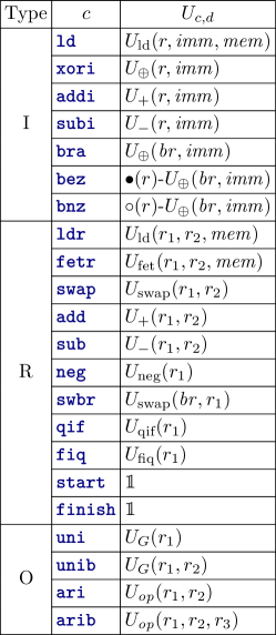
Figure 13: Full list of unitaries $U_{c,d}$ for implementing instructions in QINS.

In Section 3.3, we have shown the list of instructions in the low-level language QINS and their classical effects in Figure 5(a). We have also presented several selected examples of instructions and their corresponding implementation unitaries in Figure 5(b). In this appendix, we provide further details.

Let us first have more discussions about the classical effects of instructions in Figure 5(a).

• Load instructions are used to retrieve information (including instructions and data) from the QRAM. In particular, ld(r,i) swaps the value $M_{i}$ at address $i$ specified by the immediate number and the value in register $r$. ldr(r₁,r₂) works similarly with the address specified by the value in register $r_{2}$. fetr(r₁,r₂) instead copies (via the XOR operator $\oplus$) the value $M_{i}$ at address $i$ specified by the immediate number into register $r$.

• Unitary gate instructions are used to apply elementary quantum gates (chosen from the fixed set $\mathcal{G}$, specified by $\mathbf{RQC}^{++}$ in Section A.2.4) on registers. In particular, uni(G,r₁) applies the single-qubit unitary gate specified by $G$ on register $r_{1}$. unib(G,r₁,r₂) applies the two-qubit unitary gate specified by $G$ on registers $r_{1}$ and $r_{2}$.

• Arithmetic instructions are used to perform word-level elementary arithmetic operations, including reversible and (possibly) irreversible ones (see also Definition 5).

  Reversible arithmetic includes XOR ( xori and xor), addition ( addi and add), subtraction ( subi and sub), negation ( neg) and swap ( swap). These arithmetic operations can also take the immediate number $i$ as one of the inputs.

  A constant number of flexible choices of irreversible arithmetic operations is also allowed. In particular, ari(op,r₁,r₂) copies (by the XOR operator $\oplus$) the result of $\left\lparen\mathit{op}\ r_{2}\right\rparen$ into register $r_{1}$, where $\mathit{op}$ specifies an unary arithmetic operation. arib(op,r₁,r₂,r₃) works similarly with the $\mathit{op}$ specifying a binary arithmetic operation. In both cases, we assume $\mathit{op}\in\mathcal{O}\mathcal{P}$ for a fixed set $\mathcal{O}\mathcal{P}$ of $O(1)$ size (see also Definition 5). Here, the irreversible arithmetic operations are actually implemented reversibly by introducing garbage data.

• Branch instructions are used to realise transfer of control flow. In particular, bra(i) copies (by the XOR operator $\oplus$) the branch offset $i$ specified by the immediate number $i$ into register $\mathit{br}$. bez(r,i) and bnz(r,i) are conditional versions of bra: the former performs bra when the value in register $r$ is zero; while the latter works in the non-zero case. swbr(r) swaps the values in register $r$ and register $\mathit{br}$.

• Qif instructions are used to update the registers $\mathit{qifv}$ and $\mathit{qifw}$. Their effects are already described in Section 6.

• Special instructions are used to specify the start and finishing points of the main program.

Now we provide more details of implementing instructions in QINS. Recall that to execute an instruction stored in register $\mathit{ins}$, the quantum register machine performs a unitary

$$U_{\textup{dec}}=\sum_{c}\ket{c}\!\bra{c}\otimes\sum_{d}\ket{d}\!\bra{d}\otimes U_{c,d},$$

which is previously defined in Figure 5(b). Here, $c$ ranges over possible values of the section $\mathit{opcode}$ (see Figure 5(b)) of $\mathit{ins}$, which corresponds to the name of the instruction in $\mathit{ins}$. Depending on the type (I/R/O) of the instruction (indicated by $c$; see Figure 5(b)), $d$ ranges over possible values of other sections in $\mathit{ins}$:

• If the instruction is of type I, then $d$ ranges over possible values of the section $\mathit{reg}$ in $\mathit{ins}$.

• If the instruction is of type R, then $d$ ranges over possible values of the sections $\mathit{reg}_{1}$ and $\mathit{reg}_{2}$ in $\mathit{ins}$.

• If the instruction is of type O, then $d$ ranges over possible values of the sections $\mathit{para}$, $\mathit{reg}_{1}$, $\mathit{reg}_{2}$ and $\mathit{reg}_{3}$ in $\mathit{ins}$.

In Figure 13, we present the full list of unitaries $U_{c,d}$ for implementing instructions in QINS. Most unitaries on the third columns are defined in Definition 5. The unitaries $U_{\textup{qif}}$ and $U_{\textup{fiq}}$ for implementing instructions qif and fiq are already defined in Section 6.

Appendix C Details of Compilation

In this appendix, we provide further details of the compilation of quantum recursive programs written in the language $\mathbf{RQC}^{++}$.

C.1 Details of High-Level Transformations

In Section 4.1, we have shown a series of high-level transformations to be performed in Figure 6, and only selected the first two steps for illustration. Now we delineate every step in the high-level transformations, as well as the simplified program syntax after each step. Note that the last four steps shown in Sections C.1.3, C.1.4, C.1.5 and C.1.6 are rather simple and standard (see e.g., the textbook [1]), but we describe them in our context (adapted to support some features of the language $\mathbf{RQC}^{++}$) for completeness.

C.1.1 Replacing Quantum Branches by Procedure Calls

The first step is to replace the programs used in every quantum branch of the $\mathbf{qif}$ statements by procedure calls. We already showed this step in Section 4.1.1. For every $\mathbf{qif}$ statement, if $C_{0},C_{1}$ are not procedure identifiers or $\mathbf{skip}$ statements, then we perform the replacement:

$$\mathbf{qif}[q](\ket{0}\rightarrow C_{0})\square(\ket{1}\rightarrow C_{1})\mathbf{fiq}\qquad\Rightarrow\qquad\mathbf{qif}[q](\ket{0}\rightarrow P_{0})\square(\ket{1}\rightarrow P_{1})\mathbf{fiq},$$

where $P_{0},P_{1}$ are fresh procedure identifiers, and we add new procedure declarations $P_{i}\Leftarrow C_{i}$ (for $i\in\left\{0,1\right\}$) to $\mathcal{P}$. If only one of $C_{0},C_{1}$ is procedure identifier or $\mathbf{skip}$, then we only perform the replacement for the other branch. Note that Conditions 1, 2 and 3 are kept after this step. In particular, Condition 2 promises that $\mathit{fcv}(C_{0},\sigma)=\mathit{fcv}(C_{1},\sigma)=\emptyset$ for any classical state $\sigma$, which therefore implies the newly introduced procedure declarations $P_{i}\Leftarrow C_{i}$ satisfy Condition 3.

After this step, the program $\mathcal{P}=\left\{P(\overline{u})\Leftarrow C\right\}_{P}$ has the following simplified syntax:

$$\begin{split}C::=&\ \mathbf{skip}\mid\overline{x}:=\overline{t}\mid U\left[\overline{q}\right]\mid C_{0};C_{1}\mid P(\overline{t})\mid\mathbf{if}\ b\ \mathbf{then}\ C_{0}\ \mathbf{else}\ C_{1}\ \mathbf{fi}\mid\mathbf{while}\ b\ \mathbf{do}\ C\ \mathbf{od}\\ &\mid\mathbf{begin}\ \mathbf{local}\ \overline{x}:=\overline{t};C\ \mathbf{end}\mid\mathbf{qif}\left[q\right](\ket{0}\rightarrow P_{0})\square(\ket{1}\rightarrow P_{1})\mathbf{fiq}.\end{split}$$ (5)

C.1.2 Unrolling Nested Block Statements

The second step is to unroll all nested block statements. We already showed this step in Section 4.1.2. After this step, we are promised that the program no longer contains block statements, but when the program is implemented, we need to perform uncomputation of classical variables at the end of every procedure body for the program to preserve its original semantics. To this end, for every procedure declaration $P\left\lparen\overline{u}\right\rparen\Leftarrow C^{\prime}\in\mathcal{P}$ and every block statement $B$ appearing in $C^{\prime}$, we perform the replacement:

$$B\equiv\mathbf{begin}\ \mathbf{local}\ \overline{x}:=\overline{t};\ C\ \mathbf{end}\qquad\Rightarrow\qquad\overline{x^{\prime}}:=\overline{x};C;\overline{x}:=\overline{x^{\prime}},$$

where $\overline{x^{\prime}}$ is a list of fresh variables. Moreover, we need to append $\overline{x^{\prime}}:=\overline{0}$ at the beginning of $C^{\prime}$.

After this step, the program $\mathcal{P}=\left\{P(\overline{u})\Leftarrow C\right\}_{P}$ has the following simplified syntax:

$$\begin{split}C::=&\ \mathbf{skip}\mid\overline{x}:=\overline{t}\mid U\left[\overline{q}\right]\mid C_{0};C_{1}\mid P(\overline{t})\mid\mathbf{if}\ b\ \mathbf{then}\ C_{0}\ \mathbf{else}\ C_{1}\ \mathbf{fi}\mid\mathbf{while}\ b\ \mathbf{do}\ C\ \mathbf{od}\\ &\mid\mathbf{qif}\left[q\right](\ket{0}\rightarrow P_{0})\square(\ket{1}\rightarrow P_{1})\mathbf{fiq}.\end{split}$$ (6)

It is worth mentioning again that at this point, the semantics of the language defined by 6 is slightly changed (and different from 5) as uncomputation are needed at the end of every procedure body, but the semantics of the program $\mathcal{P}$ is preserved. The uncomputation is to be automatically done in the high-to-mid-level translation (see Section 4.2).

C.1.3 Removing Expressions in Conditions and Parameters

The third step is to remove the expression $b$ in every $\mathbf{if}$ statement and every $\mathbf{while}$ loop, and the list of expressions $\overline{t}$ in every procedure call $P\left\lparen\overline{t}\right\rparen$. After this step, classical expressions only appear in the assignment statements $\overline{x}:=\overline{t}$ and the subscriptions of variables and procedure identifiers.

• For every $\mathbf{if}$ statement, we perform the replacement:

  $$\mathbf{if}\ b\ \mathbf{then}\ C_{0}\ \mathbf{else}\ C_{1}\ \mathbf{fi}\qquad\Rightarrow\qquad x:=b;\mathbf{if}\ x\ \mathbf{then}\ C_{0}\ \mathbf{else}\ C_{1}\ \mathbf{fi}$$

  where $x$ is a fresh boolean variable.

• For every $\mathbf{while}$ statement, we perform the replacement:

  $$\mathbf{while}\ b\ \mathbf{do}\ C\ \mathbf{od}\qquad\Rightarrow\qquad x:=b;\mathbf{while}\ x\ \mathbf{do}\ C;x:=b\ \mathbf{od}$$

  where $x$ is a fresh boolean variable.

• For every procedure call $P\left\lparen\overline{t}\right\rparen$, we perform the replacement:

  $$P\left\lparen\overline{t}\right\rparen\qquad\Rightarrow\qquad\overline{x}:=\overline{t};P\left\lparen\overline{x}\right\rparen,$$

  where $\overline{x}$ is a list of fresh variables.

After this step, the program $\mathcal{P}=\left\{P(\overline{u})\Leftarrow C\right\}_{P}$ has the following simplified syntax:

$$\begin{split}C::=&\ \mathbf{skip}\mid\overline{x}:=\overline{t}\mid U\left[\overline{q}\right]\mid C_{0};C_{1}\mid P(\overline{x})\mid\mathbf{if}\ x\ \mathbf{then}\ C_{0}\ \mathbf{else}\ C_{1}\ \mathbf{fi}\mid\mathbf{while}\ x\ \mathbf{do}\ C\ \mathbf{od}\\ &\mid\mathbf{qif}\left[q\right](\ket{0}\rightarrow P_{0})\square(\ket{1}\rightarrow P_{1})\mathbf{fiq}.\end{split}$$

C.1.4 Removing Simultaneous Assignments

The fourth step is to remove every simultaneous assignment $\overline{x}:=\overline{t}$ by converting it to a series of unary assignments $x:=t$. To do this, for every $\overline{x}:=\overline{t}$ with $\overline{x}\equiv x_{1},x_{2},\ldots,x_{n}$ and $\overline{t}\equiv t_{1},t_{2},\ldots,t_{n}$, we perform the replacement

$$\begin{split}&\overline{x}:=\overline{t}\end{split}\qquad\Rightarrow\qquad\begin{split}&x_{1}^{\prime}:=t_{1};\ldots;x_{n}^{\prime}:=t_{n};\\ &x_{1}:=x_{1}^{\prime};\ldots;x_{n}:=x_{n}^{\prime};\end{split}$$

where $x_{1}^{\prime},\ldots,x_{n}^{\prime}$ are fresh variables.

After this step, the program $\mathcal{P}=\left\{P(\overline{u})\Leftarrow C\right\}_{P}$ has the following simplified syntax:

$$\begin{split}C::=&\ \mathbf{skip}\mid x:=t\mid U\left[\overline{q}\right]\mid C_{0};C_{1}\mid P(\overline{x})\mid\mathbf{if}\ x\ \mathbf{then}\ C_{0}\ \mathbf{else}\ C_{1}\ \mathbf{fi}\mid\mathbf{while}\ x\ \mathbf{do}\ C\ \mathbf{od}\\ &\mid\mathbf{qif}\left[q\right](\ket{0}\rightarrow P_{0})\square(\ket{1}\rightarrow P_{1})\mathbf{fiq}.\end{split}$$

C.1.5 Removing Expressions in Subscriptions

The fifth step is to remove expressions in the subscriptions of subscripted variables. Note that subscripted quantum variables only appear in the $U[\overline{q}]$ statements and the $\mathbf{qif}[q]\left\lparen\ket{0}\rightarrow C_{0}\right\rparen\square\left\lparen\ket{1}\rightarrow C_{1}\right\rparen\mathbf{fiq}$ statements, and subscripted procedure identifiers only appear in the procedure calls $P\left\lparen\overline{x}\right\rparen$. By the previous steps of high-level transformations, subscripted classical variables only appear in the assignments $x:=t$ and the subscriptions of quantum variables and procedure identifiers.

1. For every unitary gate statement $U\left[\overline{q}\right]$, suppose that subscripted quantum variables appearing in it are $q_{1}[e_{1}],\ldots,q_{n}[e_{n}]$ (by our assumption in Section A.2.4, $n\leq 2$), where $q_{1},\ldots,q_{n}$ are quantum arrays and $e_{1},\ldots,e_{n}$ are expressions. We perform the replacement:

   $$\begin{split}&U\left[\overline{q}\right]\end{split}\qquad\Rightarrow\qquad\begin{split}&x_{1}:=e_{1};\ldots;x_{n}:=x_{n};\\ &\left\lparen U\left[q\right]\right\rparen\left[e_{1}\leftarrow x_{1},\ldots,e_{n}\leftarrow x_{n}\right],\end{split}$$

   where $x_{1},\ldots,x_{n}$ are fresh variables, and $\left\lparen U\left[\overline{q}\right]\right\rparen\left[e_{1}\leftarrow x_{1},\ldots,e_{n}\leftarrow x_{n}\right]$ represents replacing every expression $e_{i}$ in the subscription by variable $x_{i}$ in the statement $U\left[\overline{q}\right]$.

2. For every $\mathbf{qif}[q]\left\lparen\ket{0}\rightarrow C_{0}\right\rparen\square\left\lparen\ket{1}\rightarrow C_{1}\right\rparen\mathbf{fiq}$ statement with $q=q^{\prime}[e]$ for some quantum array $q^{\prime}$ and expression $e$, we perform the replacement:

   $$\mathbf{qif}[q]\left\lparen\ket{0}\rightarrow C_{0}\right\rparen\square\left\lparen\ket{1}\rightarrow C_{1}\right\rparen\mathbf{fiq}\qquad\Rightarrow\qquad x:=e;\mathbf{qif}\left[q^{\prime}[x]\right]\left\lparen\ket{0}\rightarrow C_{0}\right\rparen\square\left\lparen\ket{1}\rightarrow C_{1}\right\rparen\mathbf{fiq},$$

   where $x$ is a fresh variable.

3. For every procedure call $P\left\lparen\overline{x}\right\rparen$ (note that at this point, actual parameters in procedure calls are variables) with $P=Q[t]$ for some procedure array $Q$ and expression $t$, we perform the replacement:

   $$P\left\lparen\overline{x}\right\rparen\qquad\Rightarrow\qquad y:=t;Q[y]\left\lparen\overline{x}\right\rparen,$$

   where $x$ is a fresh variable.

4. For every classical assignment $x:=t$, suppose that subscripted classical variables appearing in it are $y_{1}[e_{1}],y_{2}[e_{2}],\ldots,y_{n}[e_{n}]$, where $y_{1},\ldots,y_{n}$ are classical arrays and $e_{1},\ldots,e_{n}$ are expressions. We perform the replacement:

   $$\begin{split}&x:=t\end{split}\qquad\Rightarrow\qquad\begin{split}&z_{1}:=e_{1};\ldots;z_{n}:=e_{n};\\ &\left\lparen x:=t\right\rparen\left[e_{1}\leftarrow z_{1},\ldots,e_{n}\leftarrow z_{n}\right],\end{split}$$

   where $z_{1},\ldots,z_{n}$ are fresh variables, and $\left\lparen x:=t\right\rparen\left[e_{1}\leftarrow z_{1},\ldots,e_{n}\leftarrow z_{n}\right]$ represents replacing every expression $e_{i}$ in the subscription by variable $z_{i}$ in the assignment $x:=t$. Note that here $e_{1},\ldots,e_{n}$ no more contain subscripted classical variables because of our assumption in Section A.1.4.

After this step, every subscription in the program will be a classical variable.

C.1.6 Reducing Variables in Expressions

The sixth step is to replace every assignments $x:=t$ with $t$ involving multiple variables by a series of equivalent assignments

$$x_{1}:=t_{1};\ \ldots\ x_{n}:=t_{n};\ x:=t_{n+1},$$

such that every expression $t_{i}$ contains at most two variables; that is, either $t_{i}\equiv a\ \mathit{op}\ b$, where $a$ and $b$ are variables or constants, and $\mathit{op}\in\mathcal{O}\mathcal{P}$ (see also Definition 5) is an elementary binary operator; or $t_{i}\equiv\mathit{op}\ a$, where $a$ is a variable or constant, and $\mathit{op}\in\mathcal{O}\mathcal{P}$ is an elementary unary operator. We will not bother describing the details of this standard conversion.

This step is the last step of the high-level transformations. The transformed program is denoted by $\mathcal{P}_{h}=\left\{P\left\lparen\overline{u}\right\rparen\Leftarrow C\right\}_{P}$, and has the following simplified syntax:

$$\begin{split}C::=&\ \mathbf{skip}\mid x:=t\mid U\left[\overline{q}\right]\mid C_{0};C_{1}\mid P(\overline{x})\mid\mathbf{if}\ x\ \mathbf{then}\ C_{0}\ \mathbf{else}\ C_{1}\ \mathbf{fi}\mid\mathbf{while}\ x\ \mathbf{do}\ C\ \mathbf{od}\\ &\mid\mathbf{qif}\left[q\right](\ket{0}\rightarrow P_{0})\square(\ket{1}\rightarrow P_{1})\mathbf{fiq}.\end{split}$$

Moreover, every subscripted variable and procedure identifier has a basic classical variable as its subscription (e.g., $z[x],q[y],P[w]$), and every expression has the form $t\equiv\mathit{op}\ x$ or $t\equiv x\ \mathit{op}\ y$.

C.2 Details of High-Level to Mid-Level Translation

In Section 4.2, we have presented selected examples of the high-to-mid-level translation. Now we provide further details of the translation, as well as the full translation of the quantum multiplexor program previously shown in Figure 1 (part of the translation already presented in Figure 8).

We use $\mathrm{mid}\left\{D\right\}$ to denote the high-to-mid-level translation of a statement (or declaration) $D$ in the high-level language $\mathbf{RQC}^{++}$. The definition of $\mathrm{mid}\left\{\cdot\right\}$ is recursive, which further involves $\mathrm{init}\left\{\cdot\right\}$ and $\mathrm{uncp}\left\{\cdot\right\}$: the former stands for the initialisation of formal parameters in procedure declarations, and the latter stands for the uncomputation of classical variables (as required by the slightly changed program semantics after high-level transformations in Section C.1; see also the beginning of Section 4.1).

In Figure 14, we present the full list of the high-to-mid-level translation $\mathrm{mid}\left\{\cdot\right\}$, as well as the initialisation $\mathrm{init}\left\{\cdot\right\}$ and the uncompuation $\mathrm{uncp}\left\{\cdot\right\}$. We further explain as follows.

• For $D\equiv\mathbf{skip}\mid C_{1};C_{2}\mid U[q]\mid U[q_{1}q_{2}]$, the translation $\mathrm{mid}\left\{D\right\}$ and uncomputation $\mathrm{uncp}\left\{D\right\}$ of are self-explanatory. Note that our uncomputation is only for classical variables.

• For $D\equiv x:=\mathit{op}\ y\mid x:=y\ \mathit{op}\ z$, in the translation $\mathrm{mid}\left\{D\right\}$, the standard technique of introducing garbage data in reversible computing [43, 10] is used. We first compute the new value of $x$ into a fresh variable $w$, then swap the values of $x$ and $w$. Finally, the old value of $x$ will be pushed into the stack. The uncomputation $\mathrm{uncp}\left\{D\right\}$ is simply the inverse of $\mathrm{mid}\left\{D\right\}$.

• For $D\equiv\mathbf{if}\ x\ \mathbf{then}\ C_{1}\ \mathbf{else}\ C_{2}\ \mathbf{fi}$, the construction of $\mathrm{mid}\left\{D\right\}$ is inspired by [4]. Note that by the high-level transformation in Section C.1.3, variable $x$ is not changed by $C_{1}$ and $C_{2}$, So, we can use the value of $x$ to determine which branch ($x=0,1$) the control flow has run through. Here, the mid-level instruction brc (a variant of bra) is used in pair with conditional branch instructions bez and bnz to indicate the variable $x$ for the condition, which will be helpful later in the mid-to-low-level translation. The uncomputation $\mathrm{uncp}\left\{D\right\}$ is similarly constructed.

• For $D\equiv\mathbf{qif}[q]\left\lparen\ket{0}\rightarrow C_{0}\right\rparen\square\left\lparen\ket{1}\rightarrow C_{1}\right\rparen\mathbf{fiq}$, the translation $\mathrm{mid}\left\{D\right\}$ is similar to that of the $\mathbf{if}$ statement.

  What is new is our introduction of a pair of instructions qif(q) and fiq(q), which indicate the creation and join of quantum branching controlled by the quantum coin $q$. They are relevant to operations on the qif table in the partial evaluation (described in Section 5) and the execution (described in Section 6). Note that the uncomputation $\mathrm{uncp}\left\{D\right\}$ of the $\mathbf{qif}$ statement is $\emptyset$ due to Condition 2 in Section 2.3: there are no free changed variables and therefore the uncomputation of classical variables is not required.

• For $D\equiv\mathbf{while}\ x\ \mathbf{do}\ C\ \mathbf{od}$, in the translation $\mathrm{mid}\left\{D\right\}$, a fresh variable $y$ is introduced to records the number of steps taken in the loop. Note that by the high-level transformation in Section C.1.3, $x$ is not changed by $C$. So, we can use the value of $x$ and $y$ to determine where the control flow comes from. The construction of the uncomputation $\mathrm{uncp}\left\{D\right\}$ exploits the same fresh variable $y$ as the one in $\mathrm{mid}\left\{D\right\}$.

• For $D\equiv P(\overline{x})$, in the translation $\mathrm{mid}\left\{D\right\}$, we first push $n$ actual parameters $x_{1},\ldots,x_{n}$ into the stack. Then, we branch to the declaration of the procedure $P$, whose address is specified by the variable $P.\mathit{ent}$. Finally, when the procedure call is returned, we pop the actual parameters from the stack. Note that the procedure $P$ here can be subscripted, e.g., $P=Q[y]$ for some procedure array $Q$ and variable $y$. In this case, $P.\mathit{ent}=Q.\mathit{ent}[y]$ is also subscripted. The uncomputation $\mathrm{uncp}\left\{D\right\}=\emptyset$, due to Condition 3 in Section 2.3.

• For $D\equiv P(\overline{u})\Leftarrow C$, we need to handle the initialisation of formal parameters $\overline{u}$ and the automatic uncomputation of classical variables at the end of the procedure body $C$ (see Section C.1). The design of control flow in the translation $\mathrm{mid}\left\{D\right\}$ is inspired by that in the translation of classical reversible languages [4]. Specifically, the entry point and exit point to the declaration of procedure $P$ are the same, specified by $P.\mathit{ent}$. Instruction swbr is used to update the return offset register $\mathit{ro}$ (at both entry and exit), whose value will be temporarily pushed into the stack (see also Section 3.2.1) for supporting recursive procedure calls.

  What is new here is our automatic uncomputation of classical variables, done by $\mathrm{uncp}\left\{C\right\}$ at the end of the procedure body $C$.

• The initialisation $\mathrm{init}\left\{\overline{u}\right\}$ of formal parameters $\overline{u}$ is rather standard: we simply pop the actual parameters from the stack, then update the formal parameters, followed by pushing their old values into the stack.

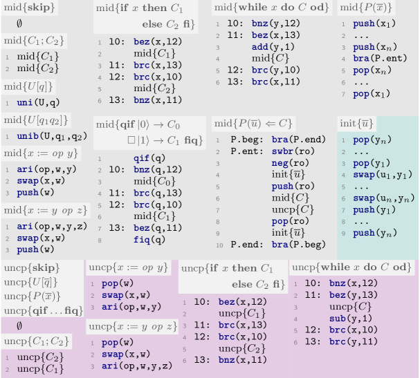
Figure 14: Full list of the high-to-mid-level translation $\mathrm{mid}\left\{\cdot\right\}$. Here, $\mathrm{init}\left\{\cdot\right\}$ and $\mathrm{uncp}\left\{\cdot\right\}$ denote the initialisation of formal parameters and uncomputation of classical variables, respectively.

Now let us apply the high-to-mid-level translation to the transformed quantum multiplexor program on the LHS of Figure 8. This yields the translated program in Figure 15, which is annotated to show the correspondence with the program on the LHS of Figure 8. For simplicity of presentation, we have also done some manual optimisation on the translated program.

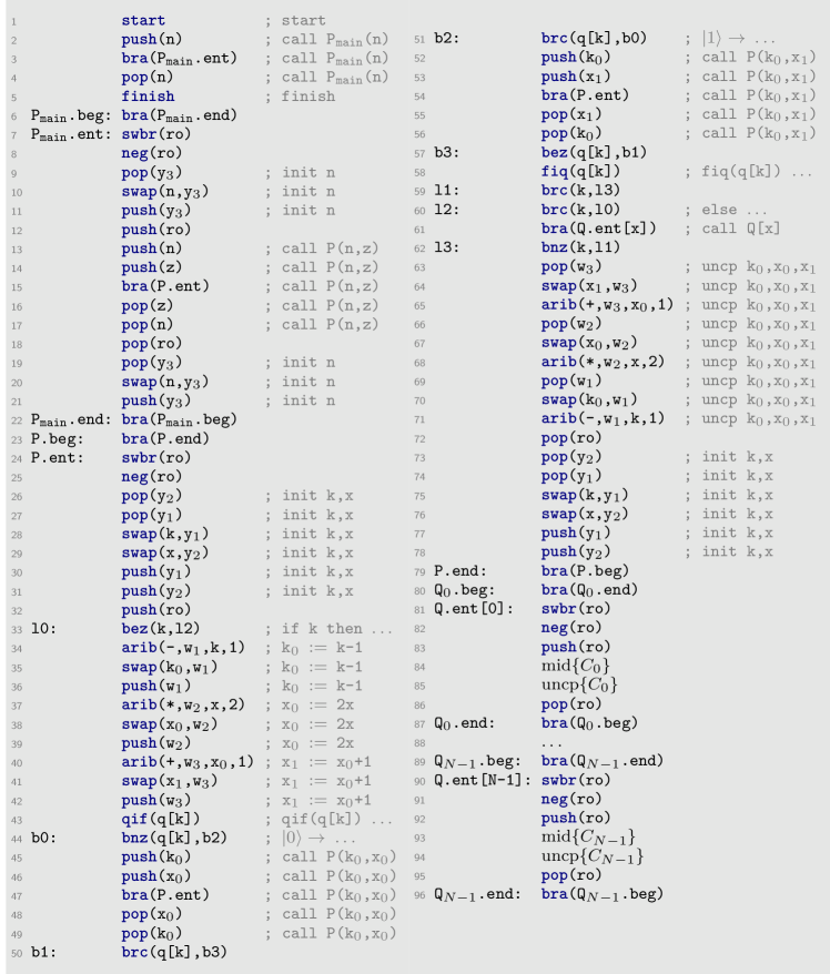
Figure 15: Full high-to-mid-level translation of the quantum multiplexor program. The original program is in Figure 1, with part of the high-to-mid-level translation previously presented in Figure 8.

C.3 Symbol Table and Memory Allocation of Variables

In Section 4.3, we only briefly mentioned the memory allocation of variables and how the symbol table will be used at runtime. In the following, we provide more details of the symbol table and memory allocation.

After the high-level to mid-level translation, we can determine the names of all variables and procedure identifiers by scanning the whole program in the mid-level language, because the mid-to-low-level translation will no more introduce new variables or procedure identifiers. The addresses of all variables (corresponding to their names) will be stored in the symbol table and loaded into the QRAM for the addressing of variables at runtime.

For classical (either basic or array) variable $x$, we use $@x$ to denote the address of the variable name $x$, which falls in the symbol table section of the QRAM (see Section 3.2.1). The memory location at address $@x$ stores $\&x$, which stands for the address of the variable $x$. If $x$ is an array variable, then $\&x$ will be the base address of $x$; i.e., $\&x=\&\left\lparen x[0]\right\rparen$. As an address, $\&x$ falls in the classical variable section of the QRAM, and stores the value of $x$. The same convention applies to any quantum variable.

Figure 16: Example of the symbol table and memory allocation of variables in the QRAM.

An example of the symbol table is visualised in Figure 16. Here, the symbol table section is composed of classical and quantum symbols. The memory location in the QRAM with address $@x$ stores $\&x$, which is the address of the memory location that stores $x[0]$, for classical array variable $x$. Similarly, for quantum variable $q$, the memory location with address $@q$ stores $\&q$, which is the address of the memory location that stores $q$.

Note that the sizes of classical and quantum arrays (except those classical variables $P.\mathit{ent}$ that correspond to procedure arrays $P$) are not determined at compile time as the classical inputs are not yet given. So, the values in the symbol table (i.e., addresses of all variables) need to be filled in after the classical inputs are considered (e.g., during the partial evaluation described in Section 5). Still, for every classical variable $x$, the address $@x$ of the name $x$ is determined. The same holds for every quantum variable. Therefore, the compiled program will be completely determined and independent of classical and quantum inputs.

C.4 Details of Mid-Level to Low-Level Translation

In Section 4.3, we have presented selected examples of the mid-to-low-level translation. In the following, we provide further details of the translation, as well as the final compiled quantum multiplexor program (the original program was previously in Figure 1).

Recall that instructions in the mid-level language can take variables and labels as inputs, while the instructions in the low-level language QINS do not. To this end, we will use load instructions ld, ldr and fetr in QINS to first load variables from the QRAM into registers, and then execute the instruction, followed by storing the results back to the QRAM. Also, the mid-level language has additional instructions push, pop and brc that need to be further translated.

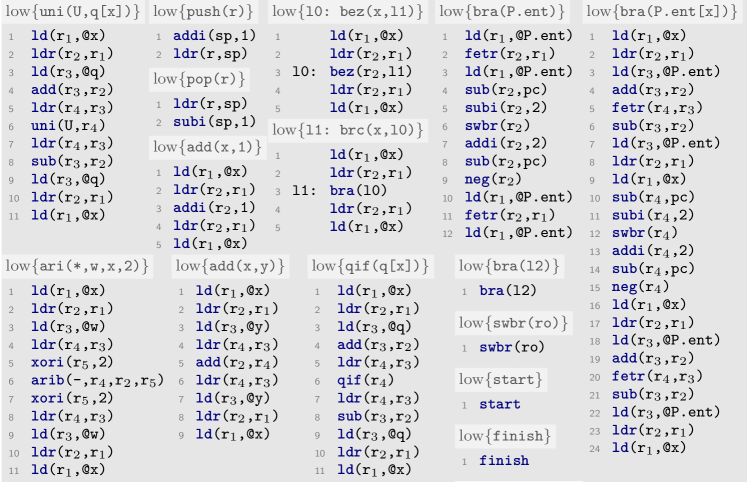
Figure 17: More examples of the mid-to-low-level translation. Here, all registers $r_{i}$ are free registers.

We use $\mathrm{low}\left\{i\right\}$ to denote the mid-to-low-level translation of a mid-level instruction $i$. In Figure 17, we present more examples of the mid-to-low-level translation. Further explanations are as follows.

• In the translation $\mathrm{low}\left\{\textup{{\color[rgb]{0,0,0.5} push}}\texttt{(r)}\right\}$, Line 1 first increments the stack pointer $\mathit{sp}$ by $1$. Then, Line 2 loads the topmost stack element (whose address is specified by $\mathit{sp}$) into free register $r$. The translation $\mathrm{low}\left\{\textup{{\color[rgb]{0,0,0.5} pop}}\texttt{(r)}\right\}$ works similarly.

• In the translation $\mathrm{low}\left\{\texttt{l0:\ }\textup{{\color[rgb]{0,0,0.5} bez}}\texttt{(x,l1)}\right\}$, Lines 1–2 first load the value of variable $x$ into free register $r_{2}$. Then, Line 3 branches to label $l0$, conditioned on $x\neq 0$. Finally, Lines 4–5 reverse the effects of Lines 1–2.

  Note that instruction l1:  brc(x,l0) is used in pair with instruction l0:  bez(x,l1). So, the free registers used in the translations $\mathrm{low}\left\{\texttt{l1:\ }\textup{{\color[rgb]{0,0,0.5} brc}}\texttt{(x,l0)}\right\}$ and $\mathrm{low}\left\{\texttt{l0:\ }\textup{{\color[rgb]{0,0,0.5} bez}}\texttt{(x,l1)}\right\}$ are also related (the same). This correspondence promises that registers $r_{1},r_{2}$ are properly cleared (hence become free again) after being used.

• In the translation $\mathrm{low}\left\{\textup{{\color[rgb]{0,0,0.5} add}}\texttt{(x,1)}\right\}$, Lines 1–2 first load the value of variable $x$ into free register $r_{2}$. Then, Line 3 adds $1$ to $r_{2}$ to obtain $x+1$. Finally, Lines 4–5 reverse the effects of Lines 1–2. Note that we use addi in Line 3, because $1$ is an immediate number.

  In comparison, in the translation $\mathrm{low}\left\{\textup{{\color[rgb]{0,0,0.5} add}}\texttt{(x,y)}\right\}$, we use add in Line 5, because both $x,y$ are variables and loaded into registers.

• In the translation $\mathrm{low}\left\{\textup{{\color[rgb]{0,0,0.5} ari}}\texttt{(*,w,x,2)}\right\}$, Lines 1–4 first load the values of $w$ and $x$ into free registers $r_{2}$ and $r_{4}$, respectively. Then, Line 5 prepares the immediate number $2$ in free register $r_{5}$. Line 6 performs the binary arithmetic operation $*$ and puts the result $x*2$ into register $r_{4}$. Finally, Lines 7–11 reverse the effects of Lines 1–4

• For instructions like bra(l2), swbr(ro), start and finish that are already in QINS, no further translation is needed.

• In the translation $\mathrm{low}\left\{\textup{{\color[rgb]{0,0,0.5} bra}}\texttt{(P.ent[x])}\right\}$, Lines 1–2 first load the value of $x$ into free register $r_{2}$. Then, the base address $\&P.\mathit{ent}$ of classical array $P.\mathit{ent}$ is loaded into $r_{3}$ by Line 3, which is added to $r_{2}$ by Line 4 to obtain the address $\&P.\mathit{ent}[x]$ of the subscripted variable $P.\mathit{ent}[x]$. Line 5 loads the value of $P.\mathit{ent}[x]$ to $r_{4}$, where fetr instead of ldr is used to preserve the copy of $P.\mathit{ent}[x]$ in the QRAM for supporting recursive procedure calls. Lines 6–9 reverse the effects of Lines 1–4.

  Lines 10–11 calculate in $r_{4}$ the offset of $P.\mathit{ent}[x]$ from the address of Line 12, which branches to the declaration of the subscripted procedure $P[x]$. Note that after Line 12, all previously used registers are cleared and become free again. Finally, Lines 13–24 reverse the effects of Lines 1–12.

Now let us apply the mid-to-low-level translation to the quantum multiplexor program in Figure 15 after the high-to-mid-level translation. This yields the full compiled program in Figure 18, which is also annotated to show the correspondence with the mid-level program in Figure 15. As usual, for simplicity of presentation, manual optimisation has been done on the translated program.

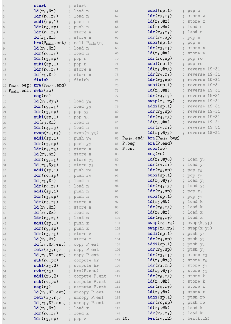
Figure 18: Full compiled quantum multiplexor program, after the mid-to-low-level translation.

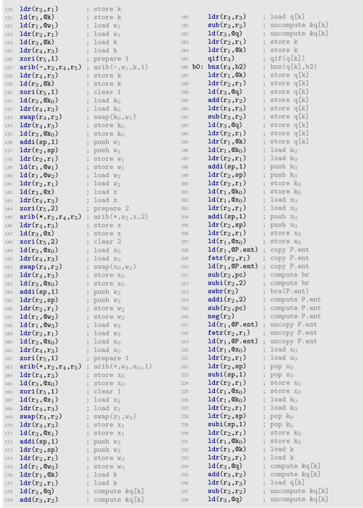
Figure 19: Full compiled quantum multiplexor program, after the mid-to-low-level translation (cont.)

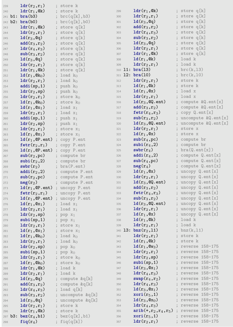
Figure 20: Full compiled quantum multiplexor program, after the mid-to-low-level translation (cont.)

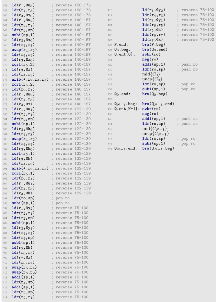
Figure 21: Full compiled quantum multiplexor program, after the mid-to-low-level translation (cont.)

Appendix D Details of Partial Evaluation

In this appendix, we present further details of the partial evaluation of compiled quantum recursive programs, in addition to Section 5.

D.1 Memory Allocation of Qif Table

In Section 5.1, we have identified the synchronisation problem in executing quantum recursive programs, and defined in Section 5.2 a data structure called qif table that will be used in superposition at runtime to address this problem. The qif table generated from the partial evaluation needs to be loaded into the QRAM at runtime. To store a qif table in the QRAM, we need an encoding of every node and its relevant information (links and counter). The simplest way to encode is to gather all information of a node into a $9$-tuple

$$\left\lparen v.w,v.\mathit{nx},v.\mathit{fc}_{0},v.\mathit{fc}_{1},v.\mathit{lc}_{0},v.\mathit{lc}_{1},v.\mathit{pr},v.\mathit{cf},v.\mathit{cl}\right\rparen.$$ (7)

Here, we assume every node $v$ is identified by its base address of the above tuple in the QRAM. For nodes of type $\circ$, some of the entries in 7 might be empty and set to $0$. In this way, the whole qif table is encoded into an array of tuples, each corresponding to a node within. Accessing the information of a node can be done in a way similar to accessing an array element. For example, if every entry in 7 occupies a word, then given the base address $a$ of a tuple that corresponds to a node $v$, one can access the information $v.\mathit{nx}$ by the address $a+1$. In Section 6, the quantum register machine might need to access the value of $v.\mathit{nx}$ (see e.g., Algorithm 3), which in this case can be fetched into a free register $r$ for later computation, by applying the unitary $U_{\mathit{fet}}(r,a+1,\mathit{mem})$.

It is worth mentioning that more compact ways (with smaller space complexity) of encoding the qif table other than the straightforward encoding in 7 exist but are not discussed here, for simplicity of presentation.

D.2 Qif Table for the Quantum Multiplexor Program

In Section 5.2, we have presented an example of an artifitial program and its corresponding qif table in Figure 11. For illustration, in Figure 22, we show the qif table for the quantum multiplexor program as another example. The original program written in $\mathbf{RQC}^{++}$ was already presented in Figure 1, while the full compiled program was shown in Figure 18. Here, we choose $n=3$. As usual, we only show the links $\mathit{fc}_{i}$ (colored in black), $\mathit{lc}_{i}$ (colored in red and dashed) and $\mathit{nx}$ (colored in blue and squiggled), while $w$, $\mathit{cf}$, $\mathit{cl}$ and $\mathit{pr}$ are omitted for simplicity. For the quantum multiplexor program, the qif table is just a tree of depth $3$, because there are only nested instantiations of the $\mathbf{qif}$ statements.

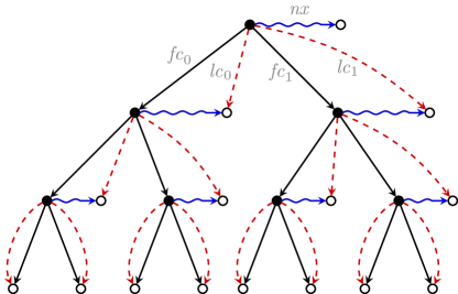
Figure 22: The qif table for the quantum multiplexor program in Figure 1, when $n=3$.

D.3 Details of Qif Table Generation

In Section 5.2.2, we have presented Algorithm 1 of the partial evaluation of quantum control flows and the generation of qif table. In the following, let us give a more detailed explanation of Algorithm 1.

Recall that Algorithm 1 is run by multiple parallel processes. We start with one initial process evaluating the function QEva. At the beginning, the program counter $\mathit{pc}$ is initialised to the starting address of the compiled main program (i.e., the address of instruction start) and the counter $t$ is initialised to $0$. An new node $v$ is created in the qif table as the initial node. In the generation of the qif table, all new nodes created are of type $\circ$, which can later become nodes of type $\bullet$ if needed. The function QEva then repeats Lines 3–16, as long as the running time $t$ does not exceed the practical running time, i.e., $t\leq T_{\textup{prac}}\left\lparen\mathcal{P}\right\rparen$. The repetition consists of the following three stages, which also appear in the execution on quantum register machine (see Section 6).

1. (Fetch):

   In this stage, register $\mathit{ins}$ is updated with the current instruction $M_{\mathit{pc}}$ whose address is specified by register $\mathit{pc}$. The counter $t$ then increments by $1$.

2. (Decode & Execute):

   In this stage, we classically emulate the behaviour of the quantum register machine, given the classical inputs. In particular, we neglect unitary gate instructions uni and unib as they involve the quantum inputs.

   1. If $\mathit{ins}=\textup{{\color[rgb]{0,0,0.5} qif}}\texttt{(q)}$, then we meet a creation of quantum branching, controlled by the quantum coin $q$. In this case, two new nodes $v_{0}$ and $v_{1}$ are created in the qif table, and are then linked with the current node $v$. Since $v_{0}$ and $v_{1}$ are from the first enclosed nested instantiation of $\mathbf{qif}\ldots\mathbf{fiq}$ of $v$, by Definition 2, we have $v.\mathit{fc}_{i}=v.\mathit{lc}_{i}=v_{i}$ for $i=0,1$. The inverse links are created similarly. Next, we fork the current process QEva into two sub-processes QEva₀ and QEva₁, which go into the quantum branches $q=0$ and $q=1$ (corresponding to $\ket{0}\rightarrow\ldots$ and $\ket{1}\rightarrow\ldots$ in the $\mathbf{qif}$ statement), respectively. For each QEva_i, the current node $v$ is updated by the children node $v_{i}$.

   2. If $\mathit{ins}=\textup{{\color[rgb]{0,0,0.5} fiq}}\texttt{(q)}$, then we meet a join of quantum branching, controlled by the quantum coin $q$. This implies the current process is a sub-process forked from some parent process. So, we wait for the pairing sub-process QEva^′ with the same parent node; i.e., $v^{\prime}.\mathit{cl}=v.\mathit{cl}=\hat{v}$ for some $\hat{v}$, where $v^{\prime}$ denotes the current node of QEva^′, and $\hat{v}$ denotes the parent node of $v$ and $v^{\prime}$. Let $\hat{t}$ be the maximum $\max\left\{t,t^{\prime}\right\}$ of the numbers of instructions in executing the two quantum branches (corresponding to $q=0,1$). Given $\hat{t}$, we can calculate $v.w=\hat{t}-t$ and $v^{\prime}.w=\hat{t}-t^{\prime}$, the numbers of instruction cycles one needs to wait at the nodes $v$ and $v^{\prime}$, respectively. Note that one of $v.w$ and $v^{\prime}.w$ will be $0$. These wait counter information will be used to synchronise the two quantum branches at runtime (see Section 6).

      After collecting the information in two quantum branches, the current process QEva will be merged with the pairing process QEva^′ into one process by updating $t$ with $\hat{t}$ and $v$ with $\hat{v}$.

      Finally, we need to create a new node $u$ in the qif table for the continuing quantum branch. We link the nodes $v$ and $u$ via $\mathit{nx}$ and $\mathit{pr}$. According to Definition 2, node $u$ will be updated as the new last children node for the parent node $\hat{u}$ of the current node $v$. Then, we move the current node from $v$ to $u$. Note that the default type of $u$ is $\circ$, and it can become $\bullet$ if later we meet a continuing non-nested instantiation of $\mathbf{qif}\ldots\mathbf{fiq}$.

   3. If $\mathit{ins}=\textup{{\color[rgb]{0,0,0.5} finish}}$, then we have finished the execution of the program, and can return the counter $t$ as the actual running time.

   4. Otherwise, if $\mathit{ins}$ is any instruction other than the unitary gate instructions uni and unib, we update the involved registers and memory locations in $M$ according to Figure 5(a).

3. (Branch):

   In this stage, we update the program counter $\mathit{pc}$ according to the branch offset $\mathit{br}$. As previously mentioned in Section 3.1, if $\mathit{br}=0$, then we increment $\mathit{pc}$ by $1$; if $\mathit{br}\neq 0$, then we update $\mathit{pc}$ with $\mathit{pc}+\mathit{br}$.

If the program $\mathcal{P}$ does not terminate within the practical time $T_{\textup{prac}}\left\lparen\mathcal{P}\right\rparen$, Algorithm 1 returns a timeout error. Otherwise, it returns the actual running time $t$, denoted by $T_{\textup{exe}}\left\lparen\mathcal{P}\right\rparen$, which will be used in the execution on quantum register machine (see Section 6).

It is worth stressing again that in the partial evaluation, only those quantum variables $q$ involved in the quantum control flows (specifically, qif(q) and fiq(q)) and all classical variables need to be evaluated; while all other quantum variables are ignored. The parallel processes for running Algorithm 1 are completely classical. One can also make use of this fact to dynamically maintain the classical registers and memory $M$ for every evaluation process, in order to save the space complexity, but we will not discuss the details here for simplicity.

D.4 Complexity Analysis of Partial Evaluation

Now let us analyse the time complexity of the partial evaluation of quantum control flows and generation of qif table described by Algorithm 1, in terms of classical parallel elemetnary operations. Our goal is to show that Algorithm 1 can be implemented using $O\left\lparen T_{\textup{exe}}\left\lparen\mathcal{P}\right\rparen\right\rparen$ classical parallel elementary operations, which will be explained as follows.

To clarify what is meant by “elementary” here, recall that all registers, the memory and the qif table in Algorithm 1 are simulated on a classical computer and stored in a classical RAM. We regard any operation that involves a constant number of memory locations in the classical RAM as an elementary operation. For example, in Algorithm 1, an operation on classical registers (including system registers $\mathit{pc},\mathit{ins},\mathit{br},\mathit{sp},v,t$ and user registers), an access to the classical memory $M$, or creation of a node in the qif table will all be regarded as a classical elementary operation.

The meaning of “parallel” here is the common one in parallel computing. Multiple elementary operations performed simultaneously are counted as one parallel elementary operation. The parallelism can appear within a single process; e.g., when a process forks into two sub-processes, its data can be copied in a parallel way, for initialising both sub-processes. The parallelism can also appear among multiple processes; e.g., when two sub-processes run simultaneously before being merged, they can perform operations in parallel. We will not bother further going down to the rigorous details.

To prove our goal, note that Algorithm 1 terminates without timeout error if and only if $t=T_{\textup{exe}}\left\lparen\mathcal{P}\right\rparen$. So, it suffices to verify that every step of a process (among other parallel processes) executing QEva can be implemented using $O\left\lparen 1\right\rparen$ classical elementary operations, as follows.

• Consider those steps in Algorithm 1 only involving registers, the memory and the qif table; e.g, $t\leftarrow 0$ in Line 1, $\mathit{ins}\leftarrow M_{\mathit{pc}}$ in Line 3, and the creation of nodes $v_{0},v_{1}$ in Line 5. It is easy to verify that each of them only involves a constant number of memory locations in the classical RAM, and therefore can be implemented by $O\left\lparen 1\right\rparen$ elementary operations.

• Consider those steps in Algorithm 1 involving forking and merging of sub-processes, in particular, Line 6 and Line 9. For the forking of a parent process into two sub-processes, we need to create a copy of all registers and the memory of the parent process. This can be done using $O\left\lparen 1\right\rparen$ classical parallel elementary operations. Similarly, for the merging of two pairing sub-processes, taking the data from any of the two sub-processes and updating registers according to Line 9 can be done using $O(1)$ classical parallel elementary operations.

Appendix E Details of Execution on Quantum Register Machine

In this appendix, we present further details of execution on quantum register machine, in addition to Section 6. Recall that the execution is the last step of implementing quantum recursive programs and the only step that concerns the quantum inputs and requires quantum hardware. At this point, the original program written in the language $\mathbf{RQC}^{++}$ is compiled into a low-level program $\mathcal{P}$ composed of instructions in QINS. We are promised that $\mathcal{P}$ terminates and has running time $T_{\textup{exe}}\left\lparen\mathcal{P}\right\rparen$, and we have generated its corresponding qif table that can be used to solve the synchronisation problem during the execution. Along the way, we have also set up a symbol table and allocated memory locations for classical and quantum variables. All these instructions and data are now loaded into the QRAM, according to the layout described in Section 3.2.1.

E.1 Details of Unitary $U_{\textup{cyc}}$ and Unitary $U_{\textup{exe}}$

In Section 6.1, we have presented in Algorithm 2 the construction of the unitary $U_{\textup{cyc}}$ applied repeatedly by the quantum register machine for each instruction cycle at runtime. We have also briefly explained unitary $U_{\textup{exe}}$ as a subroutine of $U_{\textup{cyc}}$. Now let us provide a more detailed explanation of Algorithm 2.

The execution on quantum register machine described by Algorithm 2 consists of repeated cycles, each performing the unitary $U_{\textup{cyc}}$. From the partial evaluation in Algorithm 1, we already obtain the running time $T_{\textup{exe}}\left\lparen\mathcal{P}\right\rparen$ of the compiled program $\mathcal{P}$, so we can fix the number of repetitions to be $T_{\textup{exe}}=T_{\textup{exe}}\left\lparen\mathcal{P}\right\rparen$. Before the repetitions of $U_{\textup{cyc}}$, we also need to initialise system registers $\mathit{pc},\mathit{sp},\mathit{qifv}$ according to Section 3.1. All other registers are initialised to $\ket{0}$.

For each instruction cycle, in $U_{\textup{cyc}}$, we need to decide whether to wait (i.e., skip the current instruction cycle) or execute, according to the wait counter information stored in the current node (specified by register $\mathit{qifv}$) in the qif table. To reversibly implement this procedure, we exploit two additional registers $\mathit{qifw}$ and $\mathit{wait}$, and unitary $U_{\textup{cyc}}$ is designed to consist of the following three stages.

1. (Set wait flag):

   In this stage, we check whether the value $w$ in the wait counter register $\mathit{qifw}$ is $>0$, which records the number of cycles to be skipped at the current node. At this point, we are promised that the wait flag register $\mathit{wait}$ is in state $\ket{0}$. If the wait counter $w>0$, then we set a wait flag in register $\mathit{wait}$ by flipping it to state $\ket{1}$, which indicates that the machine needs to wait at the current node.

2. (Execute or wait):

   In this stage, conditioned on the wait flag in $\mathit{wait}$, we decide whether to wait (i.e., skip the current cycle), or apply the unitary $U_{\textup{exe}}$ (defined in Algorithm 2 and explained later) to execute. If the wait flag is $0$, then we apply $U_{\textup{exe}}$. If the wait flag is $1$, then we decrement the wait counter $w$ in register $\mathit{qifw}$ by $1$.

3. (Clear wait flag):

   In this stage, we clear the wait flag in register $\mathit{wait}$, conditioned on the value $w$ in register $\mathit{qifw}$ and the counter information $v.w$, where $v$ is the value of register $\mathit{qifv}$ that specifies the current node in the qif table. Specially, if $w<v.w$, which implies that we have set the wait flag in the first stage, then we need to clear the wait flag. Note that $v.w$ is stored in the qif table, and we need to first apply the unitary $U_{\textup{fet}}$ (see Definition 1) to fetch it into some free register before using it, of which details are omitted for simplicity. After this stage, we are guaranteed that the wait flag register $\mathit{wait}$ is in state $\ket{0}$.

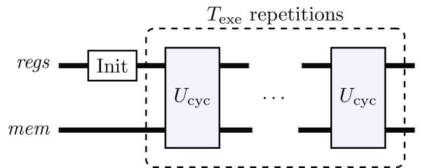
(a) $U_{\textup{main}}$. Here, $\mathit{regs}$ stands for the collection of system and user registers.

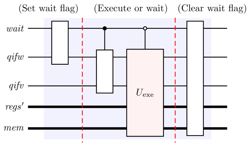
(b) $U_{\textup{cyc}}$. Here, $\mathit{regs}^{\prime}=\mathit{regs}-\mathit{wait}-\mathit{qifw}-\mathit{qifv}$.

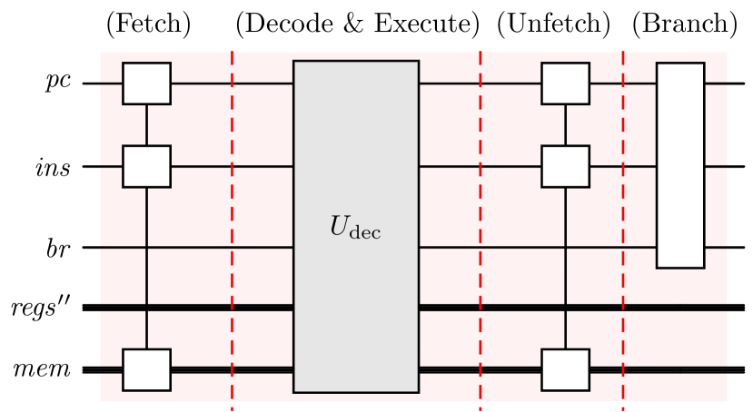
(c) $U_{\textup{exe}}$. Here, $\mathit{regs}^{\prime\prime}=\mathit{regs}-\mathit{wait}-\mathit{pc}-\mathit{ins}-\mathit{br}$.

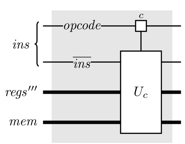
(d) $U_{\textup{dec}}$. Here, $\mathit{regs}^{\prime\prime\prime}=\mathit{regs}-\mathit{wait}-\mathit{ins}$; $\mathit{opcode}$ is the first several qubits of $\mathit{ins}$ (see Section 3.3), and $\overline{\mathit{ins}}=\mathit{ins}-\mathit{opcode}$.

Figure 23: Visualisation of the execution on quantum register machine in the form of quantum circuits. Here, unitaries $U_{\textup{main}}$, $U_{\textup{cyc}}$ and $U_{\textup{exe}}$ are defined in Algorithm 2, while $U_{\textup{dec}}$ is defined in Figure 5(b). A single wire in these quantum circuits stands for a quantum word, or a part of a quantum word, while a bundled wire stands for multiple quantum words.

As a subroutine of $U_{\textup{cyc}}$, the unitary $U_{\textup{exe}}$ consists of the following four stages.

1. (Fetch):

   In this stage, we fetch into register $\mathit{ins}$ the current instruction, whose address is specified by the program counter $\mathit{pc}$. At this point, we are promised that $\mathit{ins}$ is in state $\ket{0}$. So, we simply apply the QRAM fetch unitary $U_{\textup{fet}}\left\lparen\mathit{ins},\mathit{pc},\mathit{mem}\right\rparen$ defined in Definition 1.

2. (Decode & Execute):

   In this stage, we decode the current instruction in $\mathit{ins}$, and execute it by applying the unitary

   $$U_{\textup{dec}}=\sum_{c}\ket{c}\!\bra{c}\otimes\sum_{d}\ket{d}\!\bra{d}\otimes U_{c,d}$$

   previously defined in Figure 5(b). The full list of unitaries $U_{c,d}$ for implementing different instructions are already shown in Figure 13. What remains unspecified in Figure 13 are the unitaries $U_{\textup{qif}}$ and $U_{\textup{fiq}}$ for qif instructions qif and fiq, which are defined in Algorithm 3 and will be explained in detail later in Section E.2.

3. (Unfetch):

   In this stage, we clear the register $\mathit{ins}$ by applying the unitary $U_{\textup{fet}}\left\lparen\mathit{ins},\mathit{pc},\mathit{mem}\right\rparen$ again. After this stage, register $\mathit{ins}$ is guaranteed to be in state $\ket{0}$.

4. (Branch):

   In this stage, we update the program counter $\mathit{pc}$ according to the branch offset register $\mathit{br}$. Specifically, if the value $y$ in $\mathit{br}$ is non-zero, then we add the offset $y$ to the value in $\mathit{pc}$; otherwise, we simply increment the value in $\mathit{pc}$ by $1$.

To sum up, in Figure 23, we visualise the execution on quantum register machine (described by Algorithm 2) in the form of quantum circuits, which could be more familiar to the quantum computing community.

E.2 Details of Unitary $U_{\textup{qif}}$ and $U_{\textup{fiq}}$

In Section 6.2, we have presented in Algorithm 3 the construction of the unitaries $U_{\textup{qif}}$ and $U_{\textup{fiq}}$ for executing qif instructions, which are used in defining the unitary $U_{\textup{dec}}$ in Figure 5(b) (see also the full list of unitaries $U_{c,d}$ for implementing different instructions in Figure 13). Now we provide further explanation of Algorithm 3.

• Unitary $U_{\textup{qif}}(q)$.

  When the current instruction is qif(q), we first move the current node specified by $\mathit{qifv}$ to its first children node corresponding to the quantum coin $q$. Specifically, conditioned on the value $x$ of the quantum coin $q$, for the current node $v$ in register $\mathit{qifv}$, we first compute into some free register $r$ its first children $v.\mathit{fc}_{x}$ (corresponding to $x$); then use the inverse link $\mathit{cf}$ to clear the garbage data $v$. A following swap unitary $U_{\textup{swap}}$ finishes this move of the current node. Note that the free register $r$ is cleared at this point.

  Then, we update the wait counter register $\mathit{qifw}$ with the counter information $v.w$ stored in the qif table, where $v$ is the current node in register $\mathit{qifv}$. Here, we are promised that $\mathit{qifw}$ is initially in state $\ket{0}$, because $U_{\textup{qif}}$ is used as a subroutine of $U_{\textup{exe}}$, which will only be performed by $U_{\textup{cyc}}$ when the wait counter $\mathit{qifw}$ is in state $\ket{0}$.

  Note that in the above, the information $\mathit{fc}_{x}$, $\mathit{cf}$ and $w$ are stored in the qif table, and need to be fetched using $U_{\textup{fet}}$ into free registers before being used (see also Section D.1), of which details are omitted for simplicity.

• Unitary $U_{\textup{fiq}}(q)$.

  When the current instruction is fiq(q), we first move the current node specified by $\mathit{qifv}$ to its parent node. Specifically, similar to the construction of $U_{\textup{qif}}$, for the current node $v$ in register $\mathit{qifv}$, we first compute into some free register $r$ its parent $v.\mathit{cl}$; then conditioned on the value $x$ of the quantum coin $q$, clear the garbage data $v$ using the link $\mathit{lc}_{x}$. A following swap unitary $U_{\textup{swap}}$ finishes this first move of the current node.

  Then, we continue to move the current node to its next node. Specifically, we first compute into some free register $r$ the next node $v.\mathit{nx}$, where $v$ is the current node in register $\mathit{qifv}$. Next, we clear the garbage data $v$ using the inverse link $\mathit{pr}$, followed by a swap unitary $U_{\textup{swap}}$. After the above procedure, the register $r$ is also cleared.

  Similar to the case of $U_{\textup{qif}}$, the information $\mathit{cl}$, $\mathit{lc}_{x}$, $\mathit{nx}$ and $\mathit{pr}$ are stored in the qif table, and need to be fetched using $U_{\textup{fet}}$ into free registers before being used (see also Section D.1), of which details are omitted for simplicity.

E.3 Complexity Analysis of Execution

Now let us analyse the time complexity of the execution on quantum register machine described by Algorithm 2, in terms of quantum elementary operations. Our goal is to show that the unitary $U_{\textup{main}}$ for executing a compiled program $\mathcal{P}$ can be implemented using $O\left\lparen T_{\textup{exe}}\left\lparen\mathcal{P}\right\rparen\right\rparen$ elementary operations on registers (see Definition 5) and elementary QRAM accesses (see Definition 1).

To prove our goal, first note that the time complexity of $U_{\textup{main}}$ is dominated by the repeated applications of unitary $U_{\textup{cyc}}$. It suffices to show that unitary $U_{\textup{cyc}}$ can be implemented using $O\left\lparen 1\right\rparen$ elementary operations on registers and QRAM acesses.

Implementing $U_{\textup{cyc}}$ consists of the following steps. Let us analyse each of them.

1. (Set wait flag) in Line 4.

   It is easy to see that the unitary

   $$\sum_{w,z}\ket{w}\!\bra{w}_{\mathit{qifw}}\otimes\ket{z\oplus\left[w>0\right]}\!\bra{z}_{\mathit{wait}}$$

   can be performed using $O\left\lparen 1\right\rparen$ elementary operations on registers.

2. (Execute or wait) in Line 6.

   To implement the unitary

   $$\ket{0}\!\bra{0}_{\mathit{wait}}\otimes U_{\textup{exe}}+\sum_{z\neq 0,w}\ket{z}\!\bra{z}_{\mathit{wait}}\otimes\ket{w-1}\!\bra{w}_{\mathit{qifw}}\otimes\mathbbm{1},$$

   we first apply $\bullet\left\lparen\mathit{wait}\right\rparen$-$U_{-}\left\lparen\mathit{qifw},\mathit{r}\right\rparen$, where $U_{-}$ and $\bullet(\cdot)$-$U$ are defined in Definition 5, and $\mathit{r}$ is a free register initialised to $\ket{1}$. Then, we apply $\circ\left\lparen\mathit{wait}\right\rparen$-$U_{\textup{exe}}$, where $\circ(\cdot)$-$U$ is defined in Definition 5, and $U_{\textup{exe}}$ will be shown to be implementable using $O\left\lparen 1\right\rparen$ elementary operations on registers and QRAM accesses below. Clearing garbage data is simple and also takes $O(1)$ elementary operations.

3. (Clear wait flag) in Line 8.

   To implement the unitary

   $$\sum_{w,v,z}\ket{w}\!\bra{w}_{\mathit{qifw}}\otimes\ket{v}\!\bra{v}_{\mathit{qifv}}\ket{z\oplus\left[w<v.w\right]}\!\bra{z}_{\mathit{wait}},$$

   suppose that we use the simplest memory allocation of qif table aforementioned in Section D.1. We first apply $U_{\textup{fet}}\left\lparen r,\mathit{qifv},\mathit{mem}\right\rparen$ (defined in Definition 1) to fetch the information $v.w$ into a free register $r$, where $v$ is the value in register $\mathit{qifv}$. Given the information $v.w$ in $r$, it is easy to see that using $O\left\lparen 1\right\rparen$ elementary operations on registers we can compute $z\oplus[w<v.w]$ in register $\mathit{wait}$. Clearing garbage data is simple and also takes $O(1)$ elementary operations.

Next, we show that the unitary $U_{\textup{exe}}$ can be implemented using $O\left\lparen 1\right\rparen$ elementary operations on registers and QRAM accesses. Implementing $U_{\textup{exe}}$ consists of the following steps.

1. (Fetch) in Line 9.

   This is a simple application of $U_{\textup{fet}}$.

2. (Decode & Execute) in Line 10.

   This is an application of $U_{\textup{dec}}$, which will be shown to be implementable using $O\left\lparen 1\right\rparen$ elementary operations on registers and QRAM accesses below.

3. (Unfetch) in Line 11.

   This is a simple application of $U_{\textup{fet}}$ again.

4. (Branch) in Line 12.

   This step can be done by first applying the unitary $U_{+}$ defined in Definition 5, followed by $\circ\left\lparen\mathit{br}\right\rparen$-$U_{+}\left\lparen\mathit{pc},r\right\rparen$, where $r$ is a free register initialised to $\ket{1}$. Clearing garbage data is simple and also takes $O(1)$ elementary operations.

It remains to show that $U_{\textup{dec}}$ can be implemented using $O\left\lparen 1\right\rparen$ elementary operations on registers and QRAM accesses. Recall that $U_{\textup{dec}}$ is a quantum multiplexor $\sum_{c}\ket{c}\!\bra{c}\otimes\sum_{d}\ket{d}\!\bra{d}\otimes U_{c,d}$ (see Figure 5(b)), where the full list of unitaries $U_{c,d}$ for all instructions was presented in Figure 13. It it easy to verify that every $U_{c,d}$ can be implemented by using $O\left\lparen 1\right\rparen$ elementary operations on registers and QRAM accesses. The unitary $U_{\textup{dec}}$ can then be implemented by a sequential composition of controlled-$U_{c,d}$:

$$\ket{c}\!\bra{c}\otimes\ket{d}\!\bra{d}\otimes U_{c,d}+\sum_{c^{\prime}\neq c,d^{\prime}\neq d}\ket{c^{\prime}}\!\bra{c^{\prime}}\otimes\ket{d^{\prime}}\!\bra{d^{\prime}}\otimes\mathbbm{1}$$ (8)

for all $c,d$, each using $O\left\lparen 1\right\rparen$ elementary operations on registers and QRAM accesses. Here, $c$ ranges over possible values of the section $\mathit{opcode}$ in $\mathit{ins}$ (i.e., the names of all instructions), and $d$ ranges over possible values of other sections in $\mathit{ins}$. Since there are only $22$ distinct instructions, $O(1)$ distinct (user and system) registers, and $O(1)$ distinct parameters (in the section $\mathit{para}$ of $\mathit{ins}$; see Figure 5(b)) due to $\left\lvert\mathcal{G}\right\rvert=O(1)$ (see Section A.2.4) and $\left\lvert\mathcal{O}\mathcal{P}\right\rvert=O(1)$ (see Definition 5), the number of unitaries 8 in the sequential composition is also $O\left\lparen 1\right\rparen$. Hence, we conclude that unitary $U_{\textup{dec}}$ can be implemented using $O(1)$ elementary operations.

Appendix F Details of Efficiency and Automatic Parallelisation

In this appendix, we provide further details of the efficiency of implementing quantum recursive programs on quantum register machine as well as the automatic parallelisation, in addition to Section 7. We also present the full proof of Theorem 1 that shows the exponential parallel speed-up (over the straightforward implementation) for implementing the quantum multiplexor, obtained from the automatic parallelisation.

F.1 Quantum Circuit Complexity for Elementary Operations

In Section D.4, we have shown that the partial evaluation for a compiled program $\mathcal{P}$ can be done using $O\left\lparen T_{\textup{exe}}(\mathcal{P})\right\rparen$ classical parallel elementary operations. In Section E.3, we have shown that the execution of $\mathcal{P}$ on quantum register machine can be done using $O\left\lparen T_{\textup{exe}}(\mathcal{P})\right\rparen$ quantum elementary operations, including on registers (see Definition 5) and QRAM accesses (see Definition 1). These costs are in terms of (parallel) elementary operations. An immediate result now is that the overall parallel time complexity for implementing $\mathcal{P}$ is

$$O\left\lparen T_{\textup{exe}}\left\lparen\mathcal{P}\right\rparen\cdot\left\lparen T_{\textup{reg}}+T_{\textup{QRAM}}\right\rparen\right\rparen,$$ (9)

where $T_{\textup{reg}}$ and $T_{\textup{QRAM}}$ are the parallel time complexities for implementing an elementary operations on register and QRAM access, respectively. Here, we use the assumption that classical elementary operations are cheaper than their quantum counterparts.

The parallel time complexities $T_{\textup{reg}}$ and $T_{\textup{QRAM}}$ are further determined by how quantum elementary operations on registers and QRAM accesses are implemented at the lower level. Let us consider the more common quantum circuit model, and determine $T_{\textup{reg}}$ and $T_{\textup{QRAM}}$ when the quantum register machine is further implemented by quantum circuits.

In particular, we present the following two lemmas. The first lemma shows the quantum circuit complexity for implementing elementary operations on registers, which implies $T_{\textup{reg}}=O(\log^{2}L_{\textup{word}})$ if we consider the parallel time complexity.

Lemma 3 (Quantum circuit complexity for elementary operations on registers).

Suppose that $\mathcal{O}\mathcal{P}$ is any subset of the following set of operators: addition, subtraction, multiplication, division, cosine, sine, arctangent, exponentiation, logarithm, maximum, minimum, factorial. Then, every elementary operation on registers defined in Definition 5 can be implemented by a quantum circuit of depth $O\left\lparen\log^{2}L_{\textup{word}}\right\rparen$ and size $O\left\lparen L_{\textup{word}}^{4}\right\rparen$.

Proof.

Let us verify every elementary operation on registers in Definition 5, one by one. For simplicity of presentation, we change the order of items in Definition 5.

• (Reversible versions of possibly irreversible arithmetic): According to Lemma 5 to be presented in Appendix G, elementary arithmetic in $\mathcal{O}\mathcal{P}$ can be implemented by quantum circuits with the desired properties in Lemma 3.

• (Swap): The implementation of $U_{\textup{swap}}$ is trivially a single layer of $O\left\lparen L_{\textup{word}}\right\rparen$ parallel swap gates.

• (Unitary gate): The unitary gates in the fixed set $\mathcal{G}$ only act on one or two qubits, and can be trivially implemented.

• (Reversible elementary arithmetic):

  • The implementation of $U_{\oplus}$ is simply by a single layer of $O\left\lparen L_{\textup{word}}\right\rparen$ parallel CNOT gates.

  • The unitary $U_{+}\left\lparen r_{1},r_{2}\right\rparen$ can be implemented by first performing the mapping

    $$\ket{x}_{r_{1}}\ket{y}_{r_{2}}\ket{z}_{a}\mapsto\ket{x}_{r_{1}}\ket{y}_{r_{2}}\ket{z\oplus\left\lparen x+y\right\rparen}_{a},$$ (10)

    with $a$ being an ancilla register, followed by $U_{\textup{swap}}\left\lparen r_{1},a\right\rparen$, and finally performing the mapping

    $$\ket{x}_{r_{1}}\ket{y}_{r_{2}}\ket{z}_{a}\mapsto\ket{x}_{r_{1}}\ket{y}_{r_{2}}\ket{z\oplus\left\lparen x-y\right\rparen}_{a}.$$ (11)

    Note that 10 and 11 are elementary operations of type (Reversibly versions of possibly irreversible arithmetic) discussed above, and therefore can be implemented by a quantum circuit of depth $O\left\lparen\log^{2}L_{\textup{word}}\right\rparen$ and size $O\left\lparen L_{\textup{word}}^{4}\right\rparen$. We also have already shown that $U_{\textup{swap}}$ can be implemented by a quantum circuit of depth $O\left\lparen 1\right\rparen$ and size $O\left\lparen L_{\textup{word}}\right\rparen$. Hence, $U_{+}$ can be implemented by a quantum circuit with the desired properties in Lemma 3.

  • The implementation of $U_{-}$ is similar to that of $U_{+}$.

  • For $U_{\textup{neg}}$, if we encode an integer by recording its sign in the first bit, then implementing $U_{\textup{neg}}\left\lparen r\right\rparen$ is trivially applying an $X$ gate on the first qubit of $r$.

• (Controlled versions): Recall that we only have a constant number of registers. Suppose that an elementary operation $U$ can be implemented by a quantum circuit $Q$ of depth $O\left\lparen\log^{2}L_{\textup{word}}\right\rparen$ and size $O\left\lparen L_{\textup{word}}^{4}\right\rparen$. Then, the controlled version $\circ\left\lparen r\right\rparen$-$U$ can be implemented by first applying $\circ\left\lparen r\right\rparen$-$X\left\lparen a\right\rparen$, with $a$ being an ancilla qubit, followed by the single-controlled $c\left\lparen a\right\rparen$-$U$, and finally $\circ\left\lparen r\right\rparen$-$X\left\lparen a\right\rparen$ again. Here, $\circ\left\lparen r\right\rparen$-$X\left\lparen a\right\rparen$ is actually a multi-controlled Pauli $X$ gate, which is known to be implementable by a quantum circuit of depth $O\left\lparen\log L_{\textup{word}}\right\rparen$ and size $O\left\lparen L_{\textup{word}}\right\rparen$ (similar to, e.g., Corollary 2.5 in [85]). The single-controlled $c\left\lparen a\right\rparen$-$U$ can be implemented by replacing every gate in $Q$ by its single-controlled version, which gives a quantum circuit of depth $O\left\lparen\log^{2}L_{\textup{word}}\right\rparen$ and size $O\left\lparen L_{\textup{word}}^{4}\right\rparen$. The implementation of $\bullet\left\lparen r\right\rparen$-$U$ is similar.

  Since we only have $O\left\lparen 1\right\rparen$ registers, it is easy to see by induction that the controlled versions of any elementary operation can be implemented by a quantum circuit with the desired properties in Lemma 3.

∎

The second lemma shows the quantum circuit complexity for implementing elementary QRAM accesses, which implies $T_{\textup{QRAM}}=O\left\lparen\log N_{\textup{QRAM}}+\log L_{\textup{word}}\right\rparen$ if we consider the parallel time complexity. Using quantum circuits to implement QRAM is actually a well studied topic, for which the readers are referred to [38] for a detailed review.

Lemma 4 (Quantum circuit complexity for elementary QRAM accesses).

The elementary QRAM accesses defined in Definition 1 can be implemented by quantum circuits of depth $O\left\lparen\log N_{\textup{QRAM}}+\log L_{\textup{word}}\right\rparen$ and size $O\left\lparen L_{\textup{word}}\cdot N_{\textup{QRAM}}\log N_{\textup{QRAM}}\right\rparen$.

Proof.

We first show how to implement $U_{\textup{ld}}$. Suppose that $N=N_{\textup{QRAM}}$ and $L=L_{\textup{word}}$. Existing circuit QRAM constructions (e.g., [31, 34]) show that a QRAM of $N$ qubits can be implemented by a quantum circuit of depth $O\left\lparen\log N\right\rparen$ and size $O\left\lparen N\log N\right\rparen$. To adapt this to a QRAM of $N$ quantum words, we can use $L$ circuit QRAMs in parallel.

Specifically, the implementation of $U_{\textup{ld}}\left\lparen r,a,\mathit{mem}\right\rparen$ is as follows.

1. We first perform the unitary mapping

   $$\ket{x}_{a}\ket{y_{1}}_{a_{1}}\ldots\ket{y_{L-1}}_{a_{L-1}}\mapsto\ket{x}_{a}\ket{y_{1}\oplus x}_{a_{1}}\ldots\ket{y_{L-1}\oplus x}_{a_{L-1}},$$ (12)

   where each of $a_{1},\ldots,a_{L-1}$ is composed of $L$ ancilla qubits and initialised to $\ket{0}$. Here, 12 prepares $L$ copies of the address in $a$ (in the computational basis), and can be implemented by a quantum circuit of depth $O\left\lparen\log L\right\rparen$ and size $O\left\lparen L^{2}\right\rparen$ (see e.g., [20]).

2. Suppose that $\mathit{mem}_{i}$ is composed of the $i^{\textup{th}}$ qubit of every quantum word in our QRAM $\mathit{mem}$ (composed of quantum words). Let $r_{i}$ be the $i^{\textup{th}}$ qubit of the target register $r$, and let $a=a_{0}$. Then, we apply $U_{\textup{ld}}\left\lparen r_{i},a_{i},\mathit{mem}_{i}\right\rparen$ for $i=0$ to $L-1$ in parallel, each of which is implemented by a circuit QRAM composed of qubits, from previous works (e.g., [31, 34]). In total, this step can be implemented by a quantum circuit of depth $O\left\lparen\log N\right\rparen$ and size $O\left\lparen LN\log N\right\rparen$.

3. Finally, we perform the unitary mapping 12 again to clear the garbage data.

It is easy to verify that the above implementation satisfies the properties in Lemma 4. ∎

It turns out that $T_{\textup{reg}}$ and $T_{\textup{QRAM}}$ given by Lemmas 3 and 4 are actually small enough compared to the overall parallel time complexity for implementing quantum recursive programs. In the next section, we will make this more concrete by analysing the example of the quantum multiplexor program.

F.2 Proof of Theorem 1

Now let us analyse the complexity for implementing the quantum multiplexor program on quantum register machine, and prove Theorem 1 (whose proof sketch is already presented in Section 7). Recall that Theorem 1 shows that we can obtain an exponential parallel speed-up (over the straightforward implementation) for implementing the quantum multiplexor.

Proof of Theorem 1.

To determine the parallel time complexity, i.e., quantum circuit depth for implementing the quantum multiplexor program (see Figure 1) on quantum register machine, it suffices to determine the terms $T_{\textup{exe}}(\mathcal{P})$, $T_{\textup{reg}}$ and $T_{\textup{QRAM}}$ in 9, where $\mathcal{P}$ denotes the compiled program in Figure 18.

• To determine $T_{\textup{exe}}(\mathcal{P})$, let us analyse the partial evaluation (described by Algorithm 1) of $\mathcal{P}$. Note that Lines 1–424 of $\mathcal{P}$ are independent of $n$, in the sense that no matter how large $n$ is, this part of the program text is fixed.

  Before branching to each procedure $Q[x]$ (that describes unitary $U_{x}$ in the quantum multiplexor 1) for $x\in[N]$, the value of the counter $t$ is only determined by the number of nesting layers of $\mathbf{qif}\ldots\mathbf{fiq}$ instantiations, up to a constant factor. As the qif table of the quantum multiplexor program is a tree, as shown in Figure 22, the number of nesting layers is exactly the depth of the tree, which is equal to $n$.

  After branching to procedures $Q[x]$ for $x\in[N]$, the value of the counter $t$ is determined by the time complexity of executing every $Q[x]$. Recall that Theorem 1 assumes each $U_{x}$ is composed of $T_{x}$ elementary unitary gates, i.e., the procedure body $C_{x}$ of $Q[x]$ is composed of $T_{x}$ unitary gate instructions. So, the number of cycles to execute every $C_{x}$ is $O(T_{x})$. As Algorithm 1 is run by parallel processes, each going into a single quantum branch, the overall parallel running time is $O\left\lparen\max_{x\in[N]}T_{x}\right\rparen$.

  Combining the above together, we have

  $$T_{\textup{exe}}(\mathcal{P})=O\left\lparen\max_{x\in[N]}T_{x}+n\right\rparen.$$

• To determine $T_{\textup{reg}}$ and $T_{\textup{QRAM}}$, it suffices to determine the word length $L_{\textup{word}}$ and the QRAM size $N_{\textup{QRAM}}$ for executing the compiled program $\mathcal{P}$. Let us first determine how large $N_{\textup{QRAM}}$ is needed, by calculating the sizes (counted by the number of quantum words) of all sections in the QRAM, as follows.

  • Program section: The compiled program $\mathcal{P}$ is already presented in Figure 18, which consists of $\Theta\left\lparen\sum_{x\in[N]}T_{x}\right\rparen$ instructions.

  • Symbol table section: The size of the symbol table is upper bounded by the number of variables. By our assumption, every $C_{x}$ is composed of unitary gate instructions, so the number of variables is further upper bounded by $\Theta\left\lparen\sum_{x\in[N]}T_{x}\right\rparen$, which is the number of instructions in $\mathcal{P}$.

  • Variable section: The size of the variable section is upper bounded by $\Theta\left\lparen\sum_{x\in[N]}T_{x}\right\rparen$, as mentioned above.

  • Qif table section: The size of the qif table is easily seen to be $\Theta\left\lparen 2^{n}\right\rparen$, by noting that the qif table of $\mathcal{P}$ is a simple tree shown in Figure 22.

  • Stack section: The size of the stack is upper bounded by the number of variables and the number of nesting layers of $\mathbf{qif}\ldots\mathbf{fiq}$ instantiations, up to a constant factor. The former is upper bounded by $\Theta\left\lparen\sum_{x\in[N]}T_{x}\right\rparen$, and the latter is upper bounded by $\Theta(n)$. Hence, the overall size is upper bounded by $\Theta\left\lparen\sum_{x\in[N]}T_{x}\right\rparen$.

  To summarise, taking $N_{\textup{QRAM}}=\Theta\left\lparen\sum_{x\in[N]}T_{x}\right\rparen$ is sufficient to implement $\mathcal{P}$. Now for the word length $L_{\textup{word}}$, we only need it to be large enough to store an address of a memory location in the QRAM, as required by the formats of instructions in QINS (see Figure 5(b)). So, taking $L_{\textup{word}}=O\left\lparen\log\left\lparen N_{\textup{QRAM}}\right\rparen\right\rparen$ is enough. Finally, by Lemmas 3 and 4, we can calculate

  $$T_{\textup{reg}} =O\left\lparen\log^{2}\log N_{\textup{QRAM}}\right\rparen=O\left\lparen\log^{2}T_{\textup{QRAM}}\right\rparen,$$

  $$T_{\textup{QRAM}} =O\left\lparen\log N_{\textup{QRAM}}\right\rparen=O\left\lparen n+\log\left\lparen\max_{x\in[N]}T_{x}\right\rparen\right\rparen.$$

By inserting the above $T_{\textup{exe}}(\mathcal{P})$, $T_{\textup{reg}}$ and $T_{\textup{QRAM}}$ into 9, we obtain the overall parallel time complexity $\widetilde{O}\left\lparen n\cdot\max_{x\in[N]}T_{x}+n^{2}\right\rparen$, as desired. ∎

Appendix G Parallel Quantum Circuits for Elementary Arithmetic

In this appendix, we restate Lemma 2.6 in [85], which translates several classical results in parallel computing [52, 59, 9] into the quantum setting: elementary arithmetic functions can be efficiently approximated by classical circuits of low depth. The translation is by introducing garbage data as in standard reversible computing [43, 10]. Although these classical results are more refined, the following lemma only provides simple upper bounds for simplicity.

Lemma 5 (Parallel quantum circuits for elementary arithmetics, restating Lemma 2.6 in [85]).

Suppose $f$ is one of the following elementary arithmetic functions: addition, subtraction, multiplication, division, modulo, cosine, sine, arctangent, exponentiation, logarithm, maximum, minimum, factorial. Then, the unitary

$$\sum_{\widetilde{x},\widetilde{y},z=0}^{2^{L}-1}\ket{\widetilde{x},\widetilde{y}}\!\bra{\widetilde{x},\widetilde{y}}\otimes\ket{z\oplus\widetilde{f}\left\lparen\widetilde{x},\widetilde{y}\right\rparen}\!\bra{z}$$

can be implemented by a quantum circuit of depth $O\left\lparen\log^{2}L\right\rparen$ and size $O\left\lparen L^{4}\right\rparen$, where $\widetilde{x},\widetilde{y}$ are certain proper representations of $x,y$, and $\widetilde{f}\left\lparen\widetilde{x},\widetilde{y}\right\rparen$ is an approximation of $f\left\lparen x,y\right\rparen$ with error $2^{-L}$. Here, for unary $f$, the input $y$ is omitted. Further, if $f$ is addition, subtraction or multiplication (modulo $2^{L}$), the depth can be $O\left\lparen\log L\right\rparen$ and the error can be $0$.

It is worth mentioning the quantum circuit in Lemma 5 can use ancilla qubits. The number of ancilla qubits can be trivially upper bounded by the size $O\left\lparen L^{4}\right\rparen$ of the quantum circuit.

Appendix H More Examples of Quantum Recursive Programs

In this appendix, we provide more examples of quantum recursive programs for further illustrating the compilation process. For simplicity of presentation, we will only show the high-level transformations and the high-to-mid-level translation of these examples, while omitting the rather lengthy mid-to-low-level translation. The high-level programs for these examples are from [75].

The first example is the generation of the Greenberger-Horne-Zeilinger (GHZ) state [33]. This simple example involves recursive procedure calls but no $\mathbf{qif}$ statements.

Example 1 (Generation of GHZ states).

The (generalised) Greenberger-Horne-Zeilinger (GHZ) state [33] of $n$ qubits is defined as:

$$\ket{\textup{GHZ}(n)}=\frac{1}{\sqrt{2}}\left\lparen\ket{0}^{\otimes n}+\ket{1}^{\otimes n}\right\rparen.$$

We can use the following program in $\mathbf{RQC}^{++}$ to generate the GHZ state [75]:

$$\begin{split}P_{\textup{main}}(n)\ \Leftarrow\ &\mathbf{if}\ n=1\\ &\quad\mathbf{then}\ H\left[q[n]\right]\\ &\quad\mathbf{else}\ P_{\textup{main}}(n-1);\mathit{CNOT}\left[q[n-1],q[n]\right]\\ &\mathbf{fi}.\end{split}$$ (13)

The GHZ state generation program after the high-level transformations is presented in Figure 24, of which the high-to-mid-level translation is further shown in Figure 25. As usual, we have done some manual optimisation to improve the presentation.

$$\begin{split}P_{\textup{main}}(n)\ \Leftarrow\ &n_{0}:=n-1;\\ &\mathbf{if}\ n_{0}\ \mathbf{then}\\ &\qquad P_{\textup{main}}(n_{0});\\ &\qquad\mathit{CNOT}\left[q[n_{0}],q[n]\right]\\ &\quad\mathbf{else}\ H[q[n]]\\ &\mathbf{fi}\end{split}$$

Figure 24: The GHZ state generation program after the high-level transformations.

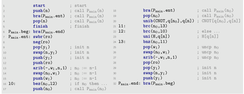
Figure 25: Full high-to-mid-level translation of the GHZ state generation program.

The second example is the multi-controlled gate. This example is still simple, but illustrates both $\mathbf{qif}$ statements and recursive procedure calls.

Example 2 (Multi-controlled Gate).

Let $U$ be an elementary unitary gate. Then the multi-controlled $U$ gate with $n-1$ control qubits is defined by:

$$C^{(*)}(U)\ket{i_{1},\ldots,i_{n-1}}\ket{\psi}=\begin{cases}\ket{i_{1},\ldots,i_{n-1}}U\ket{\psi},&i_{m}=\ldots=i_{n-1}=1,\\ \ket{i_{1},\ldots,i_{n-1}}\ket{\psi},&o.w.\end{cases}$$

for all $i_{1},\ldots,i_{n-1}\in\left\{0,1\right\}$ and quantum state $\ket{\psi}$. We can describe $C^{(*)}(U)$ by the following program in $\mathbf{RQC}^{++}$ [75]:

$$\begin{split}P_{\textup{main}}(n)\ \Leftarrow\ &P(1,n)\\ P(m,n)\ \Leftarrow\ &\mathbf{if}\ m=n\\ &\ \ \ \mathbf{then}\ U[q[n]]\\ &\ \ \ \mathbf{else}\ \mathbf{qif}[q[m]]\ket{0}\rightarrow\mathbf{skip}\\ &\quad\ \qquad\qquad\square\ \ \ \ket{1}\rightarrow P\left\lparen m+1,n\right\rparen\\ &\qquad\quad\ \mathbf{fiq}\\ &\mathbf{fi}.\end{split}$$ (14)

In Figure 26, we present the multi-controlled gate program after applying the high-level transformations to 14. Further, the full high-to-mid-level translation of the program is shown in Figure 27, which is annotated to show the correspondence with the program in Figure 26.

$$\begin{split}P_{\textup{main}}(n)\ \Leftarrow\ &y:=1;P(y,n)\\ P(m,n)\ \Leftarrow\ &x:=n-m;\\ &\mathbf{if}\ x\ \mathbf{then}\\ &\qquad m_{0}:=m+1;\\ &\qquad\mathbf{qif}[q[m]]\ket{0}\rightarrow\mathbf{skip}\\ &\qquad\qquad\square\ \ \ \ket{1}\rightarrow P\left\lparen m_{0},n\right\rparen\\ &\qquad\mathbf{fiq}\\ &\quad\mathbf{else}\ U[q[n]]\\ &\mathbf{fi}\end{split}$$

Figure 26: The multi-controlled gate program after the high-level transformations.

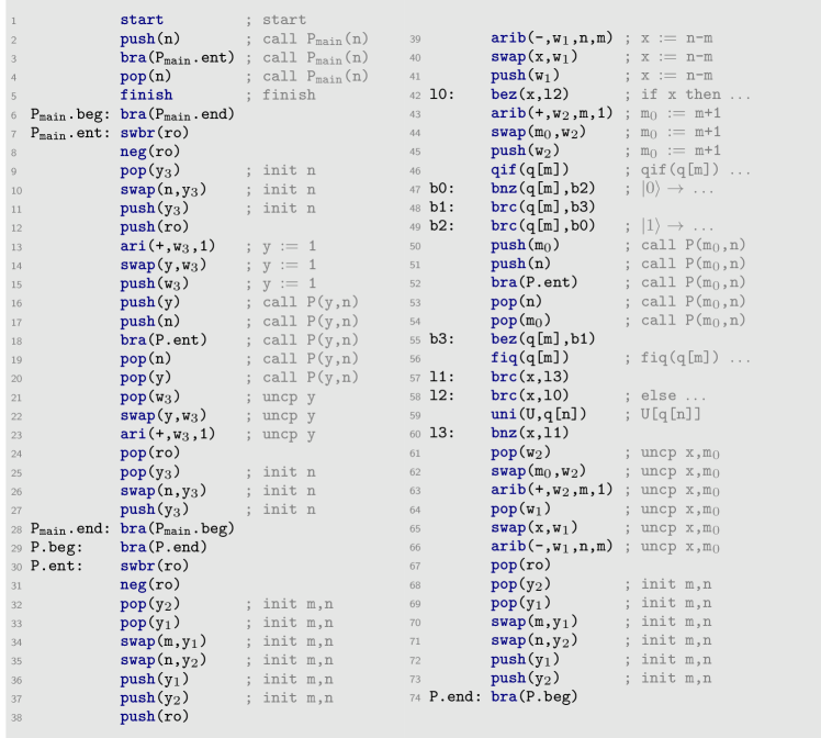
Figure 27: Full high-to-mid-level translation of the multi-controlled gate program.

The third example is the quantum state preparation, which is a common subroutine in many quantum algorithms, e.g., Hamiltonian simulation [13, 14, 42], quantum machine learning [45, 41], and solving quantum linear system of equations [36, 18]. This example involves both $\mathbf{qif}$ statements and recursive procedure calls. It also offers automatic parallelisation, resulting in a quantum circuit of poly-logarithmic depth for implementing the quantum state preparation (of which the detailed analysis is omitted), although whose complexity is slightly worse than the state-of-the-art algorithms [60, 65, 82, 81].

Example 3 (Quantum State Preparation).

The task of quantum state preparation is to generate the $n$-qubit quantum state

$$\ket{\psi}=\sum_{j\in[N]}\alpha_{j}\ket{j},$$ (15)

where $N=2^{n}$ and $\alpha_{j}\in\mathbbm{C}$ satisfy $\sum_{j\in[N]}\left\lvert\alpha_{j}\right\rvert^{2}=1$.

For $j\in[N]$, let us define $\theta_{j}\in[0,2\pi)$ such that $\alpha_{j}=e^{i\theta_{j}}\left\lvert\alpha_{j}\right\rvert$. For $l,r\in[N]$, let $S_{l,r}=\sum_{j=l}^{r}\left\lvert\alpha_{j}\right\rvert^{2}$. We define a single qubit unitary $U_{k,x}$ such that:

$$U_{k,x}\ket{0}=\sqrt{\gamma_{x}}\ket{0}+e^{i\beta_{x}}\sqrt{1-\gamma_{x}}\ket{1},$$

where $\gamma_{x}=\frac{S_{u,w-1}}{S_{u,v-1}}$, $\beta_{x}=\theta_{w}-\theta_{u}$, $u=2^{n-k}x$, $v=2^{n-k}(x+1)$ and $w=(u+v)/2$.

Now we can use the following program in $\mathbf{RQC}^{++}$ to generate the state $\ket{\psi}$ [75]:

$$\begin{split}P_{\textup{main}}(n)\ \Leftarrow\ &P(0,n,0)\\ P(k,n,x)\ \Leftarrow\ &\mathbf{if}\ k\neq n\\ &\quad\mathbf{then}\ Q(k,x)\\ &\quad\mathbf{else}\ \mathbf{qif}\left[q\left[k\right]\right]\ket{0}\rightarrow P\left\lparen k+1,n,2x\right\rparen\\ &\quad\ \qquad\qquad\square\ \ \ket{1}\rightarrow P\left\lparen k+1,n,2x+1\right\rparen\\ &\qquad\quad\ \mathbf{fiq}\\ &\mathbf{fi}\\ Q(k,x)\ \Leftarrow\ &C,\end{split}$$ (16)

where $C$ is a quantum circuit that performs $U_{k,x}[q[k+1]]$. (In practice, when the elementary gate set is simple, e.g., $\left\{H,S,T,\mathit{CNOT}\right\}$, what $C$ performs is only an approximation of $U_{k,x}$, and $C$ depends on the explicit $\alpha_{j}$ (for $j\in[N]$).)

In Figure 28, we show the quantum state preparation program after applying the high-level transformations to 16. The full high-to-mid-level translation of the program is then presented in Figure 29, where the annotation shows the correspondence with the program in Figure 28.

$$\begin{split}P_{\textup{main}}(n)\ \Leftarrow\ &z:=0;P(z,n,z)\\ P(k,n,x)\ \Leftarrow\ &y:=n-k;\\ &\mathbf{if}\ y\ \mathbf{then}\\ &\qquad k_{0}:=k+1;\\ &\qquad x_{0}:=2x;\\ &\qquad x_{1}:=x_{0}+1;\\ &\qquad\mathbf{qif}\left[q\left[k\right]\right]\ket{0}\rightarrow P\left\lparen k_{0},n,x_{0}\right\rparen\\ &\qquad\qquad\square\ \ \ket{1}\rightarrow P\left\lparen k_{0},n,x_{1}\right\rparen\\ &\qquad\mathbf{fiq}\\ &\quad\mathbf{else}\ Q(k,x)\\ &\mathbf{fi}\\ Q(k,x)\ \Leftarrow\ &C,\end{split}$$

Figure 28: The quantum state preparation program after the high-level transformations.

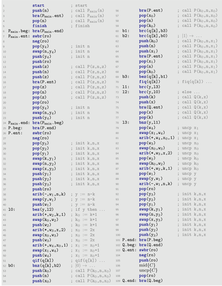
Figure 29: Full high-to-mid-level translation of the quantum state preparation program.

Appendix I Further Discussions on Related Work

I.1 The Synchronisation Problem

In Section 5, we have described the partial evaluation of quantum control flows, which is used to address (within a practical running time) the synchronisation problem (see Section 5.1) for executing programs with quantum control flows. In this appendix, we discuss some related works to the synchronisation problem.

The synchronisation problem dates back to Deutsch’s definition of quantum Turing machine [25]. In particular, Myers [51] pointed out a problem in Deutsch’s original definition: for a universal quantum Turing machine that allows inputs being in quantum superposition, different quantum branches are asynchronous and can have different termination times, where some branch might even never halt. The consequence is that one cannot check the halting of quantum Turing machine (according to Deutsch’s definition) by directly measuring a flag qubit because the measurement can destroy the superposition of different quantum branches.

A later definition of quantum Turing machine [12] given by Bernstein and Vazirani circumvented this problem by an explicit halting scheme. It requires all quantum branches to be synchronised: if any quantum branch terminates the computation at some time $T$, then all other branches also terminate at $T$. There is also a number of subsequent discussions [53, 44, 54, 63, 49, 72] about the synchronisation problem and the halting schemes of quantum Turing machine. Recently, in [80] they studied the synchronisation problem in general transition systems and formalised synchronisation as a condition.

Addressing (or circumventing) the synchronisation problem is often by restricting the inputs to be a specific subset such that different quantum branches always synchronise. For example, in [12], the synchronisation condition is explicitly stated in their definition of quantum Turing machine. In [72], they extend the definition of quantum Turing machine in [12], and show a conversion of a quantum Turing machine from the extended definition to the standard one by inserting meaningless symbols to synchronise different quantum branches. In [80], they impose structures on the program in their low-level language by borrowing the techniques of paired branch instructions from the classical reversible languages [70, 28, 5, 68], and manually insert nop (no operation) into the low-level programs to synchronise different quantum branches.

To address the synchronisation problem, in our implementation of quantum recursive programs, we exploit the structures of the programs imposed by the high-level language $\mathbf{RQC}^{++}$ (in particular, the $\mathbf{qif}$ statement for managing quantum control flows; see Section 2), and our compilation promises that the compiled low-level programs inherit the structures (via paired instructions qif and fiq in QINS; see Section 3.3). Then, we use the partial evaluation of quantum control flows to generate the qif table (see Section 5), a data structure that records the history information of quantum branching within a practical running time, which is used later (in quantum superposition) to synchronise different quantum branches at runtime (see Section 6.2). Note that our whole implementation is automatic. The technique of manually inserting nop (like in previous works [72, 80]) is not extendable to handle our case of quantum recursive programs, because the length of (dynamic) computation generated by quantum recursion cannot be pre-determined from the (static) program text.

I.2 Implementation of Quantum Multiplexor

In Theorem 1, we have shown that via the quantum register machine, we can automatically obtain a parallel implementation of the quantum multiplexor. In this appendix, we further compare it with previous efficient implementations in [82, 83].

Recall that a quantum multiplexor can be described by the unitary

$$U=\sum_{x\in[N]}\ket{x}\!\bra{x}\otimes U_{x},$$

where $N=2^{n}$ and $n$ is the number of control qubits. Let us assume all $U_{x}$ act on the last $m$ data qubits. For general $U_{x}$, it is shown in [82, Algorithm 4,5] and [83, Lemma 7] that $U$ can be implemented by a quantum circuit of depth $O\left\lparen n+\max_{x\in[N]}T_{x}\right\rparen$ and size $O\left\lparen\sum_{x\in[N]}T_{x}\right\rparen$, where each $T_{x}$ is the time for implementing controlled-$U_{x}$. The idea of their construction is similar to that of the bucket-brigade QRAM [31, 30, 35, 34].

In particular, the bucket-brigade QRAM uses a binary tree structure to route the address qubits (see Section 3.2) to the corresponding memory location. The construction in [82, 83] uses a similar structure to route the $n$ control qubits and a single data qubit to the location specified by the control qubits. Such structure is repeated $m$ times in parallel to route the total $m$ data qubits, and the first $n$ control qubits also needs to be copied (in the computational basis) $m$ times in parallel. At each location $x\in[N]$, the quantum circuit for implementing $U_{x}$ is placed. Finally, a reverse routing processes is applied to retrieve the control and data qubits. In this way, if the $n$ control qubits are in superposition, then the $m$ data qubits can travel through a superposition of paths to pass through unitaries $U_{x}$ and therefore realise the quantum multiplexor $U$.

Unlike in [82, 83] where data flows in quantum superposition, in our implementation of the quantum multiplexor, the $m$ data qubits do not move. The control structure in $U$ is completely captured by the quantum multiplexor program $\mathcal{P}$ in Figure 1, and the quantum register machine essentially realises the quantum control flows: it executes all quantum programs $C_{x}$ (that describe unitaries $U_{x}$) in quantum superposition. Indeed, the quantum register machine also exploits the circuit QRAM [31, 30, 35, 34] (see also Section F.1) at the low-level, to which the high-level programmer is oblivious.

From the perspective of design (as aforementioned in Sections 1.1 and 1.2.3), compared to the manual design of the rather involved quantum circuits in [82, 83], our Theorem 1 is automatically obtained from our implementation of quantum recursive programs. In our framework, the programmer only needs to design at high-level (in particular, the quantum multiplexor program in Figure 1), and needs not to know the explicit construction of QRAM. Not only restricted to the quantum multiplexor, the automatic parallelisation from our framework also works for general quantum recursive programs.

References

- [1] V. Alfred, S. Monica, Ravi Sethi and D. Jeffrey “Compilers: principles, techniques & tools” Pearson Education, 2007
- [2] Thorsten Altenkirch and Jonathan Grattage “A functional quantum programming language” In 20th Annual IEEE Symposium on Logic in Computer Science (LICS’05), 2005, pp. 249–258
- [3] Israel F. Araujo, Daniel K. Park, Francesco Petruccione and Adenilton J. da Silva “A divide-and-conquer algorithm for quantum state preparation” In Scientific reports 11.1, 2021, pp. 6329
- [4] Holger Bock Axelsen “Clean translation of an imperative reversible programming language” In International Conference on Compiler Construction, 2011, pp. 144–163
- [5] Holger Bock Axelsen, Robert Glück and Tetsuo Yokoyama “Reversible machine code and its abstract processor architecture” In Computer Science–Theory and Applications: Second International Symposium on Computer Science in Russia, CSR 2007, Ekaterinburg, Russia, September 3-7, 2007. Proceedings 2, 2007, pp. 56–69
- [6] Ryan Babbush, Dominic W. Berry, Ian D. Kivlichan, Annie Y. Wei, Peter J. Love and Alán Aspuru-Guzik “Exponentially more precise quantum simulation of fermions in second quantization” In New Journal of Physics 18, 2016, pp. 033032
- [7] Ryan Babbush et al. “Encoding electronic spectra in quantum circuits with linear T complexity” In Physical Review X 8.4, 2018, pp. 041015
- [8] Ryan Babbush, Nathan Wiebe, Jarrod McClean, James McClain, Hartmut Neven and Garnet Kin-Lic Chan “Low-depth quantum simulation of materials” In Physical Review X 8, 2018, pp. 011044
- [9] Paul W. Beame, Stephen A. Cook and H. Hoover “Log depth circuits for division and related problems” In SIAM Journal on Computing 15.4, 1986, pp. 994–1003
- [10] Charles H. Bennett “Logical reversibility of computation” In IBM Journal of Research and Development 17.6, 1973, pp. 525–532
- [11] Debajyoti Bera, Frederic Green and Steven Homer “Small depth quantum circuits” In ACM SIGACT News 38.2 ACM New York, NY, USA, 2007, pp. 35–50
- [12] Ethan Bernstein and Umesh Vazirani “Quantum complexity theory” In Proceedings of the twenty-fifth annual ACM symposium on Theory of computing, 1993, pp. 11–20
- [13] Dominic W. Berry, Andrew M. Childs, Richard Cleve, Robin Kothari and Rolando D. Somma “Simulating Hamiltonian dynamics with a truncated Taylor series” In Physical Review Letters 114, 2015, pp. 090502
- [14] Dominic W. Berry, Andrew M. Childs and Robin Kothari “Hamiltonian simulation with nearly optimal dependence on all parameters” In Proceedings of the 56th Annual IEEE Symposium on Foundations of Computer Science, FOCS ’15, 2015, pp. 792–809
- [15] Benjamin Bichsel, Maximilian Baader, Timon Gehr and Martin Vechev “Silq: A high-level quantum language with safe uncomputation and intuitive semantics” In Proceedings of the 41st ACM SIGPLAN Conference on Programming Language Design and Implementation, 2020, pp. 286–300
- [16] Anne Broadbent and Elham Kashefi “Parallelizing quantum circuits” In Theoretical computer science 410.26, 2009, pp. 2489–2510
- [17] Dan Browne, Elham Kashefi and Simon Perdrix “Computational depth complexity of measurement-based quantum computation” In Theory of Quantum Computation, Communication, and Cryptography: 5th Conference, TQC 2010, Leeds, UK, April 13-15, 2010, Revised Selected Papers 5, 2011, pp. 35–46
- [18] Andrew M. Childs, Robin Kothari and Rolando D. Somma “Quantum algorithm for systems of linear equations with exponentially improved dependence on precision” In SIAM Journal on Computing 46.6, 2017, pp. 1920–1950
- [19] Andrew M. Childs and Nathan Wiebe “Hamiltonian simulation using linear combinations of unitary operations” In Quantum Information & Computation 12.11–12, 2012, pp. 901–924
- [20] Richard Cleve and John Watrous “Fast parallel circuits for the quantum Fourier transform” In Proceedings of the 41st Annual IEEE Symposium on Foundations of Computer Science, FOCS ’00, 2000, pp. 526–536
- [21] Andrew W. Cross, Lev S. Bishop, John A. Smolin and Jay M. Gambetta “Open quantum assembly language”, 2017 arXiv:1707.03429 [quant-ph]
- [22] Raphael Dias da Silva, Einar Pius and Elham Kashefi “Global quantum circuit optimization”, 2013 arXiv:1301.0351 [quant-ph]
- [23] Vincent Danos, Elham Kashefi and Prakash Panangaden “The measurement calculus” In Journal of the ACM (JACM) 54.2, 2007, pp. 8–es
- [24] Haowei Deng, Runzhou Tao, Yuxiang Peng and Xiaodi Wu “A case for synthesis of recursive quantum unitary programs” In Proceedings of the ACM on Programming Languages 8, 2024, pp. 1759–1788
- [25] David Deutsch “Quantum theory, the Church–Turing principle and the universal quantum computer” In Proceedings of the Royal Society of London. A. Mathematical and Physical Sciences 400.1818, 1985, pp. 97–117
- [26] Edsger W. Dijkstra “Notes on structured programming” circulated privately, 1970 URL: http://www.cs.utexas.edu/users/EWD/ewd02xx/EWD249.PDF
- [27] Edsger W. Dijkstra “Programming considered as a human activity” In Classics in software engineering, 1979, pp. 1–9
- [28] Michael Patrick Frank “Reversibility for efficient computing”, 1999
- [29] X. Fu et al. “eQASM: An executable quantum instruction set architecture” In 2019 IEEE International Symposium on High Performance Computer Architecture (HPCA), 2019, pp. 224–237
- [30] Vittorio Giovannetti, Seth Lloyd and Lorenzo Maccone “Architectures for a quantum random access memory” In Physical Review A 78.5, 2008, pp. 052310
- [31] Vittorio Giovannetti, Seth Lloyd and Lorenzo Maccone “Quantum random access memory” In Physical review letters 100.16, 2008, pp. 160501
- [32] Frederic Green, Steven Homer, Cristopher Moore and Christopher Pollett “Counting, fanout and the complexity of quantum ACC” In Quantum Information & Computation 2.1, 2002, pp. 35–65
- [33] Daniel M. Greenberger, Michael A. Horne and Anton Zeilinger “Going beyond Bell’s theorem” In Bell’s theorem, quantum theory and conceptions of the universe Springer, 1989, pp. 69–72
- [34] Connor T. Hann, Gideon Lee, S.. Girvin and Liang Jiang “Resilience of quantum random access memory to generic noise” In PRX Quantum 2.2, 2021, pp. 020311
- [35] Connor T. Hann et al. “Hardware-efficient quantum random access memory with hybrid quantum acoustic systems” In Physical Review Letters 123.25 APS, 2019, pp. 250501
- [36] Aram W. Harrow, Avinatan Hassidim and Seth Lloyd “Quantum algorithm for linear systems of equations” In Physical Review Letters 103.15, 2009, pp. 150502
- [37] Peter Høyer and Robert Špalek “Quantum fan-out is powerful” In Theory of Computing 1.5, 2005, pp. 81–103
- [38] Samuel Jaques and Arthur G. Rattew “QRAM: A survey and critique”, 2023 arXiv:2305.10310 [quant-ph]
- [39] Jiaqing Jiang, Xiaoming Sun, Shang-Hua Teng, Bujiao Wu, Kewen Wu and Jialin Zhang “Optimal space-depth trade-off of CNOT circuits in quantum logic synthesis” In Proceedings of the 31st Annual ACM-SIAM Symposium on Discrete Algorithms, SODA ’20, 2020, pp. 213–229
- [40] Richard Jozsa “An introduction to measurement based quantum computation”, 2005 arXiv:quant-ph/0508124 [quant-ph]
- [41] Iordanis Kerenidis and Anupam Prakash “Quantum recommendation systems” In 8th Innovations in Theoretical Computer Science Conference (ITCS 2017) 67, 2017, pp. 49:1–49:21
- [42] Robin Kothari “Efficient algorithms in quantum query complexity”, 2014
- [43] Rolf Landauer “Irreversibility and heat generation in the computing process” In IBM journal of research and development 5.3, 1961, pp. 183–191
- [44] Noah Linden and Sandu Popescu “The halting problem for quantum computers”, 1998 arXiv:quant-ph/9806054 [quant-ph]
- [45] Seth Lloyd, Masoud Mohseni and Patrick Rebentrost “Quantum principal component analysis” In Nature physics 10.9, 2014, pp. 631–633
- [46] Guang Hao Low, Vadym Kliuchnikov and Luke Schaeffer “Trading T gates for dirty qubits in state preparation and unitary synthesis” In Quantum 8, 2024, pp. 1375
- [47] Guang Hao Low and Nathan Wiebe “Hamiltonian simulation in the interaction picture”, 2019 arXiv:1805.00675 [quant-ph]
- [48] Christopher Lutz and Howard Derby “Janus: a time-reversible language” In Letter to Rolf Landauer 2, 1986
- [49] Takayuki Miyadera and Masanori Ohya “On halting process of quantum turing machine” In Open Systems & Information Dynamics 12.3, 2005, pp. 261–264
- [50] Cristopher Moore and Martin Nilsson “Parallel quantum computation and quantum codes” In SIAM Journal on Computing 31.2, 2002, pp. 799–815
- [51] John M. Myers “Can a universal quantum computer be fully quantum?” In Physical Review Letters 78.9, 1997, pp. 1823
- [52] Yu Ofman “On the algorithmic complexity of discrete functions” In Sov. Math. Dokl. 7.7, 1963, pp. 589
- [53] Masanao Ozawa “Quantum nondemolition monitoring of universal quantum computers” In Physical Review Letters 80.3, 1998, pp. 631
- [54] Masanao Ozawa “Quantum Turing machines: local transition, preparation, measurement, and halting” In Quantum Communication, Computing, and Measurement 2 Springer, 1998, pp. 241–248
- [55] Anouk Paradis, Benjamin Bichsel, Samuel Steffen and Martin Vechev “Unqomp: synthesizing uncomputation in quantum circuits” In Proceedings of the 42nd ACM SIGPLAN International Conference on Programming Language Design and Implementation, 2021, pp. 222–236
- [56] Anouk Paradis, Benjamin Bichsel and Martin Vechev “Reqomp: space-constrained uncomputation for quantum circuits” In Quantum 8, 2024, pp. 1258
- [57] Einar Pius “Automatic parallelisation of quantum circuits using the measurement based quantum computing model” In High Performance Computing, 2010
- [58] Robert Raussendorf and Hans J. Briegel “A one-way quantum computer” In Physical Review Letters 86.22, 2001, pp. 5188
- [59] John H. Reif “Logarithmic depth circuits for algebraic functions” In SIAM Journal on Computing 15.1, 1986, pp. 231–242
- [60] Gregory Rosenthal “Query and depth upper bounds for quantum unitaries via Grover search”, 2023 arXiv:2111.07992 [quant-ph]
- [61] Amr Sabry, Benoît Valiron and Juliana Kaizer Vizzotto “From symmetric pattern-matching to quantum control” In Foundations of Software Science and Computation Structures: 21st International Conference, FOSSACS 2018, 2018, pp. 348–364
- [62] Vivek V. Shende, Stephen S. Bullock and Igor L. Markov “Synthesis of quantum logic circuits” In Proceedings of the 2005 Asia and South Pacific Design Automation Conference, 2005, pp. 272–275
- [63] Yu Shi “Remarks on universal quantum computer” In Physics Letters A 293.5-6, 2002, pp. 277–282
- [64] Robert S. Smith, Michael J. Curtis and William J. Zeng “A practical quantum instruction set architecture”, 2017 arXiv:1608.03355 [quant-ph]
- [65] Xiaoming Sun, Guojing Tian, Shuai Yang, Pei Yuan and Shengyu Zhang “Asymptotically optimal circuit depth for quantum state preparation and general unitary synthesis” In IEEE Transactions on Computer-Aided Design of Integrated Circuits and Systems 42.10, 2023, pp. 3301–3314
- [66] Yasuhiro Takahashi and Seiichiro Tani “Collapse of the hierarchy of constant-depth exact quantum circuits” In Proceedings of the 28th IEEE Conference on Computational Complexity, 2013, pp. 168–178
- [67] Barbara M. Terhal and David P. DiVincenzo “Adptive quantum computation, constant depth quantum circuits and arthur-merlin games” In Quantum Information & Computation 4.2, 2004, pp. 134–145
- [68] Michael Kirkedal Thomsen, Holger Bock Axelsen and Robert Glück “A reversible processor architecture and its reversible logic design” In Reversible Computation: Third International Workshop, RC 2011, Gent, Belgium, July 4-5, 2011. Revised Papers 3, 2012, pp. 30–42
- [69] Hristo Venev, Timon Gehr, Dimitar Dimitrov and Martin Vechev “Modular synthesis of efficient quantum uncomputation”, 2024 arXiv:2406.14227 [cs.PL]
- [70] Carlin James Vieri “Reversible computer engineering and architecture”, 1999
- [71] Finn Voichick, Liyi Li, Robert Rand and Michael Hicks “Qunity: A unified language for quantum and classical computing” In Proceedings of the ACM on Programming Languages 7, 2023, pp. 921–951
- [72] Qisheng Wang and Mingsheng Ying “Quantum random access stored-program machines” In Journal of Computer and System Sciences 131, 2023, pp. 13–63
- [73] Mingsheng Ying “Foundations of quantum programming” Morgan Kaufmann, 2016
- [74] Mingsheng Ying, Nengkun Yu and Yuan Feng “Defining quantum control flow”, 2012 arXiv:1209.4379 [quant-ph]
- [75] Mingsheng Ying and Zhicheng Zhang “Verification of recursively defined quantum circuits”, 2024 arXiv:2404.05934 [quant-ph]
- [76] Tetsuo Yokoyama, Holger Bock Axelsen and Robert Glück “Principles of a reversible programming language” In Proceedings of the 5th Conference on Computing Frontiers, 2008, pp. 43–54
- [77] Tetsuo Yokoyama and Robert Glück “A reversible programming language and its invertible self-interpreter” In Proceedings of the 2007 ACM SIGPLAN symposium on Partial evaluation and semantics-based program manipulation, 2007, pp. 144–153
- [78] Charles Yuan and Michael Carbin “The T-complexity costs of error correction for control flow in quantum computation” In Proceedings of the ACM on Programming Languages 8.PLDI, 2024, pp. 492–517
- [79] Charles Yuan and Michael Carbin “Tower: data structures in quantum superposition” In Proceedings of the ACM on Programming Languages 6.OOPSLA2, 2022, pp. 259–288
- [80] Charles Yuan, Agnes Villanyi and Michael Carbin “Quantum control machine: The limits of control flow in quantum programming” In Proceedings of the ACM on Programming Languages 8.OOPSLA1, 2024, pp. 1–28
- [81] Pei Yuan and Shengyu Zhang “Optimal (controlled) quantum state preparation and improved unitary synthesis by quantum circuits with any number of ancillary qubits” In Quantum 7, 2023, pp. 956
- [82] Xiao-Ming Zhang, Tongyang Li and Xiao Yuan “Quantum state preparation with optimal circuit depth: Implementations and applications” In Physical Review Letters 129.23, 2022, pp. 230504
- [83] Xiao-Ming Zhang and Xiao Yuan “Circuit complexity of quantum access models for encoding classical data” In npj Quantum Information 10.1, 2024, pp. 42
- [84] Xiao-Ming Zhang, Man-Hong Yung and Xiao Yuan “Low-depth quantum state preparation” In Physical Review Research 3.4 APS, 2021, pp. 043200
- [85] Zhicheng Zhang, Qisheng Wang and Mingsheng Ying “Parallel quantum algorithm for hamiltonian simulation” In Quantum 8, 2024, pp. 1228