Deterministic Policy Gradient Primal-Dual Methods
for Continuous-Space Constrained MDPs

Abstract

We study the problem of computing deterministic optimal policies for constrained Markov decision processes (MDPs) with continuous state and action spaces, which are widely encountered in constrained dynamical systems. Designing deterministic policy gradient methods in continuous state and action spaces is particularly challenging due to the lack of enumerable state-action pairs and the adoption of deterministic policies, hindering the application of existing policy gradient methods for constrained MDPs. To this end, we develop a deterministic policy gradient primal-dual method to find an optimal deterministic policy with non-asymptotic convergence. Specifically, we leverage regularization of the Lagrangian of the constrained MDP to propose a deterministic policy gradient primal-dual (D-PGPD) algorithm that updates the deterministic policy via a quadratic-regularized gradient ascent step and the dual variable via a quadratic-regularized gradient descent step. We prove that the primal-dual iterates of D-PGPD converge at a sub-linear rate to an optimal regularized primal-dual pair. We instantiate D-PGPD with function approximation and prove that the primal-dual iterates of D-PGPD converge at a sub-linear rate to an optimal regularized primal-dual pair, up to a function approximation error. Furthermore, we demonstrate the effectiveness of our method in two continuous control problems: robot navigation and fluid control. To the best of our knowledge, this appears to be the first work that proposes a deterministic policy search method for continuous-space constrained MDPs.

1 Introduction

Constrained Markov decision processes (MDPs) are a standard framework for incorporating system specifications into dynamical systems (Altman, 2021; Brunke et al., 2022). In recent years, constrained MDPs have attracted significant attention in constrained Reinforcement Learning (RL), whose goal is to derive optimal control policies through interaction with unknown dynamical systems (Achiam et al., 2017; Tessler et al., 2018). Policy gradient-based constrained learning methods have become the workhorse driving recent successes across various disciplines, e.g., navigation (Paternain et al., 2022), video compression (Mandhane et al., 2022), and finance (Chow et al., 2018).

This paper is motivated by two observations. First, continuous state-action spaces are pervasive in dynamical systems, yet most algorithms in constrained RL are designed for discrete state and action spaces (Achiam et al., 2017; Tsiamis et al., 2021; Altman, 2021). Second, the literature on constrained RL largely focuses on stochastic policies. However, randomly taking actions by following a stochastic policy is often prohibitive in practice, especially in safety-critical domains (Li et al., 2022; Gao et al., 2023). Deterministic policies alleviate such concerns, but (i) they might lead to sub-optimal solutions (Ross, 1989; Altman, 2021); and (ii) computing them can be NP-complete (Feinberg, 2000; Dolgov, 2005). Nevertheless, there is a rich body of constrained control literature that studies problems where optimal policies are proved to be deterministic (Posa et al., 2016; Tsiamis et al., 2020; Zhao and You, 2021; Ma et al., 2022). Viewing this gap between constrained RL and control, we study the problem of finding optimal deterministic policies for constrained MDPs with continuous state-action spaces.

A key consideration of this paper is the fact that deterministic policies are sub-optimal in finite state-action spaces, but sufficient for constrained MDPs with continuous state-action spaces (Feinberg and Piunovskiy, 2002, 2019). This enables our formulation of a constrained RL problem with deterministic policies. To develop a tractable deterministic policy search method, we introduce a regularized Lagrangian approach that leverages proximal optimization methods. Moreover, we use function approximation to ensure scalability in continuous state-action spaces. Our contribution is four-fold.

1. We introduce a deterministic policy constrained RL problem for a constrained MDP with continuous state-action spaces and prove that the problem exhibits zero duality gap, despite being constrained to deterministic policies.

2. We propose a regularized deterministic policy gradient primal-dual (D-PGPD) algorithm that updates the primal policy via a proximal-point-type step and the dual variable via a gradient descent step, and we prove that the primal-dual iterates of D-PGPD converge to a set of regularized optimal primal-dual pairs at a sub-linear rate.

3. We propose an approximation for D-PGPD by including function approximation. We prove that the primal-dual iterates of the approximated D-PGPD converge at a sub-linear rate, up to a function approximation error.

4. We demonstrate that D-PGPD addresses a classical constrained navigation problem with a range of cost functions and constraints. Moreover, we show that D-PGPD can solve non-linear fluid control problems under constraints.

Related work. Deterministic policy search has been explored in the context of unconstrained MDPs (Silver et al., 2014; Lillicrap et al., 2015; Kumar et al., 2020; Lan, 2022). However, in constrained setups, the use of deterministic policies has been restricted to occupancy measure optimization problems within finite state-action spaces (Dolgov, 2005). Our work extends deterministic policy search to constrained MDPs with continuous state-action spaces. The two main roadblocks that we overcome are: the sub-optimality of deterministic policies and the NP-completeness of computing them (Ross, 1989; Feinberg, 2000; Dolgov, 2005; Altman, 2021; McMahan, 2024). For the former, we first note that deterministic policies are sufficient in constrained MDPs with continuous state-action spaces (Feinberg and Piunovskiy, 2002, 2019), which allows us to exploit the convexity of the value image to establish strong duality in the deterministic policy space. For the latter, we employ a quadratic regularization of the reward function to propose a regularization-based primal-dual algorithm and exploit the structural properties of value functions to prove that it converges to an optimal deterministic policy in the last iterate. Last-iterate convergence analysis of primal-dual algorithms has been studied in constrained RL (Moskovitz et al., 2023; Ding et al., 2024b, a). However, these methods consider stochastic policies and are limited to finite-action spaces. In the context of control, there is a rich body of literature on continuous state-action spaces and deterministic policies in constrained setups (Scokaert and Rawlings, 1998; Lim and Zhou, 1999). However, the solutions are usually model-based and tailored to specific structured problems (Posa et al., 2016; Tsiamis et al., 2020; Zhao et al., 2021; Zhao and You, 2021; Ma et al., 2022). Bridging the gap between constrained control and RL has been explored in the past (Kakade et al., 2020; Zahavy et al., 2021; Li et al., 2023). However, these methods are model-based and focus on stochastic policies. In contrast, we propose a model-free deterministic policy search method for constrained MDPs with continuous state-action spaces.

2 Preliminaries

We consider a discounted constrained MDP, denoted by the tuple $(S,A,p,r,u,b,\gamma,\rho)$. Here, $S\subseteq{\mathbb{R}}^{d_{s}}$ and $A\subseteq{\mathbb{R}}^{d_{a}}$ are continuous state-action spaces with dimensions $d_{s}$ and $d_{a}$, and bounded actions $\|a\|\leq A_{\text{max}}$ for all $a\in A$; $p(\cdot\,|\,s,a)$ is a probability measure over $S$ parametrized by the state-action pairs $(s,a)\in S\times A$; $r$, $u$: $S\times A\mapsto[0,1]$ are reward/utility functions; $b$ is a constraint threshold; $\gamma\in[0,1)$ is a discount factor; and $\rho$ is a probability measure that specifies an initial state. We consider the set of all deterministic policies $\Pi$ in which a policy $\pi$: $S\mapsto A$ maps states to actions. The transition $p$, the initial state distribution $\rho$, and the policy $\pi$ define a probability distribution over trajectories $\{s_{t},a_{t},r_{t},u_{t}\}_{t=0}^{\infty}$, where $s_{0}\sim\rho$, $a_{t}=\pi(s_{t})$, $r_{t}=r(s_{t},a_{t})$, $u_{t}=u(s_{t},a_{t})$ and $s_{t+1}\sim p(\cdot\,|\,s_{t},a_{t})$ for all $t\geq 0$. Given a policy $\pi$, we define the value function $V^{\pi}_{r}$: $S\to{\mathbb{R}}$ as the expected sum of discounted rewards

$$V_{r}^{\pi}(s)\; \mathrel{\mathop{:}}=\;\mathbb{E}_{\pi}\left[\sum_{t=0}^{\infty}\gamma^{t}r(s_{t},a_{t})\;|\;s_{0}=s\right].$$

For the utility function, we define the corresponding value function $V^{\pi}_{u}$. Their expected values over the initial state distribution $\rho$ are denoted as $V_{r}(\pi)\mathrel{\mathop{:}}=\mathbb{E}_{\rho}[V_{r}^{\pi}(s)]$ and $V_{u}(\pi)\mathrel{\mathop{:}}=\mathbb{E}_{\rho}[V_{u}^{\pi}(s)]$, where we drop the dependence on $\rho$ for simplicity of notation. Boundedness of $r$ and $u$ leads to $V_{r}(\pi)$, $V_{u}(\pi)\in[0,1/(1-\gamma)]$. We introduce a discounted state visitation distribution $d_{s_{0}}^{\pi}(B)\mathrel{\mathop{:}}=(1-\gamma)\sum_{t\,=\,0}^{\infty}\text{Pr}(s_{t}\in B\,|\,\pi,s_{0})$ for any $B\subseteq S$ and define $d_{\rho}^{\pi}(s)\mathrel{\mathop{:}}=\mathbb{E}_{s_{0}\,\sim\,\rho}[d_{s_{0}}^{\pi}(s)]$. For the reward function $r$, we define the state-action value function $Q^{\pi}_{r}$: $S\times A\to{\mathbb{R}}$ given an initial action $a$ while following $\pi$,

$$Q_{r}^{\pi}(s,a)\;\mathrel{\mathop{:}}=\;\mathbb{E}_{\pi}\left[\sum_{t=0}^{\infty}\gamma^{t}r(s_{t},a_{t})|s_{0}=s,a_{0}=a\right].$$

We let the associated advantage function $A^{\pi}_{r}$: $S\times A\to{\mathbb{R}}$ be $A_{r}^{\pi}(s,a)\;\mathrel{\mathop{:}}=\;Q_{r}^{\pi}(s,a)-V_{r}^{\pi}(s)$. Similarly, we define $Q^{\pi}_{u}$: $S\times A\to{\mathbb{R}}$ and $A^{\pi}_{u}$: $S\times A\to{\mathbb{R}}$ for the utility function $u$.

A policy is optimal for a given reward function when it maximizes the corresponding value function. However, the value functions $V_{r}(\pi)$ and $V_{u}(\pi)$ are usually in conflict, e.g., a policy that maximizes $V_{r}(\pi)$ is not necessary good for $V_{u}(\pi)$. To trade off two conflicting objectives, constrained MDP aims to find an optimal policy $\pi^{\star}$ that maximizes the reward value function $V_{r}(\pi)$ subject to an inequality constraint on the utility value function $V_{u}(\pi)\geq b$, where we assume $b\in(0,1/(1-\gamma)]$ to avoid trivial solutions. We use a single constraint for the sake of simplicity, but our results extend to problems with multiple constraints. We translate the constraint $V_{u}(\pi)\geq b$ into the constraint $V_{g}(\pi)\geq 0$ for $g\mathrel{\mathop{:}}=u-(1-\gamma)b$, where $g$: $S\times A\mapsto[-1,1]$ denotes the translated utility. This leads to the following problem

$$\begin{array}[]{rl}\displaystyle\operatornamewithlimits{max}_{\pi\,\in\,\Pi}&\;\;V_{r}(\pi)\\[5.69046pt] \operatornamewithlimits{s.t.}&\;\;V_{g}(\pi)\;\geq\;0.\end{array}$$ (1)

Restricting Problem (1) to deterministic policies poses several challenges. Deterministic policies can be sub-optimal in constrained MDPs with finite state-action spaces (Ross, 1989; Altman, 2021), and when they exist, finding them is an NP-complete problem (Feinberg, 2000). Furthermore, Problem (1) is not convex in the policy, but when considering stochastic policies, Problem (1) can be equivalently represented in terms of occupancy measures, resulting in a linear program (Paternain et al., 2019). However, the occupancy measure representation of (1) is a non-linear and non-convex problem when only deterministic policies are considered (Dolgov, 2005). Finally, multiple policies can achieve the optimal value function $V^{\pi^{\star}}_{P}$ while satisfying the constraint. We denote the set of all maximizers of (1) that attain $V^{\pi^{\star}}_{P}$ as $\Pi^{\star}$.

To address these points, we first note that deterministic policies are sufficient in constrained MDPs with continuous state-action spaces under the following assumption (Feinberg and Piunovskiy, 2002, 2019) .

Assumption 1 (Non-atomicity).

The MDP is non-atomic, i.e., $\rho(s)=0$ and $p(s^{\prime}\,|\,s,a)=0$ for all $s$, $s^{\prime}\in S$ and $a\in A$.

Assumption 1 is mild in practice. Since stochastic perturbations are a common in physical systems with continuous state and action spaces (Anderson and Moore, 2007), the probability measures $\rho$ and $p(\cdot\,|\,s,a)$ are normally atomless, i.e., for any measurable set $B\subseteq S$ with probability measures $\rho(B)$ and $p(B\,|\,s,a)$, there exists a measurable subset $B^{\prime}\subset B$ that has smaller non-zero probability measures $\rho(B)>\rho(B^{\prime})>0$ and $p(B\,|\,s,a)>p(B^{\prime}\,|\,s,a)>0$ for any $s\in S$ and $a\in A$. In other words, the transition probability and the initial probability do not concentrate in a single state (Feinberg and Piunovskiy, 2019). When a constrained MDP is non-atomic, the set of deterministic policies is sufficient (Feinberg and Piunovskiy, 2019). Specifically, let $V(\pi)\mathrel{\mathop{:}}=[\,V_{r}(\pi)\;V_{g}(\pi)\,]^{\top}$ denote the vector of value functions for a given policy $\pi$. We define a deterministic value image ${\mathcal{V}}_{D}\mathrel{\mathop{:}}=\{V(\pi)\,|\,\pi\in\Pi\}$, which is a set of all attainable vector value functions for deterministic policies. We denote by ${\mathcal{V}}_{T}$ a value image for all policies. The deterministic value image ${\mathcal{V}}_{D}$ and the value image ${\mathcal{V}}_{T}$ are equivalent under Assumption 1 for discounted MDPs (see Lemmas 2 and 4 in Appendix B). Therefore, the optimal value function of a non-atomic constrained MDP is contained in the deterministic value image ${\mathcal{V}}_{D}$. Furthermore, the deterministic value image ${\mathcal{V}}_{D}$ is a convex set, even though each value function $V(\pi)\in{\mathcal{V}}_{D}$ is non-convex in policy $\pi$ (see Lemmas 2 and 3 in Appendix B). Below, we summarize the two aforementioned observations.

Lemma 1 (Sufficiency of deterministic policies).

For a non-atomic discounted MDP, the deterministic value image ${\mathcal{V}}_{D}$ is convex, and equals the value image ${\mathcal{V}}_{T}$, i.e., ${\mathcal{V}}_{D}={\mathcal{V}}_{T}$.

2.1 Zero Duality Gap

With the convexity of the deterministic value image ${\mathcal{V}}_{D}$ in hand, we next establish zero duality gap for Problem (1). We begin with a standard feasibility assumption.

Assumption 2 (Feasibility).

There exists a deterministic policy $\tilde{\pi}\in\Pi$ and $\xi>0$ such that $V_{g}(\tilde{\pi})\geq\xi$.

We dualize the constraint by introducing $\lambda\in\mathbb{R}^{+}$ and the Lagrangian $L(\pi,\lambda)\mathrel{\mathop{:}}=V_{r}(\pi)+\lambda V_{g}(\pi)$ for Problem (1). For a fixed $\lambda$, let $\Pi(\lambda)$ be the set of Lagrangian maximizers. The Lagrangian $L(\pi,\lambda)$ is equivalent to the value function $V_{\lambda}(\pi)$ associated with the combined reward/utility function $r_{\lambda}(s,a)=r(s,a)+\lambda g(s,a)$. The dual function $D(\lambda)\mathrel{\mathop{:}}=\operatornamewithlimits{max}_{\pi\in\Pi}V_{\lambda}(\pi)$ is an upper bound of Problem (1), and the dual problem searches for the tightest primal upper bound

$$\operatornamewithlimits{min}_{\lambda\,\in\,{\mathbb{R}}^{+}}\;D(\lambda).$$ (2)

We denote by $V_{D}^{\lambda^{\star}}$ the optimal value of the dual function, where $\lambda^{\star}$ is a minimizer of the dual Problem (2). Despite being non-convex in the policy, if we replace the deterministic policy space in Problem (1) with the stochastic policy space, then it is known that Problem (1) has zero duality gap (Paternain et al., 2019). The proof capitalizes on the convexity of the occupancy measure representation of (1) for stochastic policies. However, this occupancy-measure-based argument does not carry to deterministic policies, since the occupancy measure representation of Problem (1) is non-convex when only deterministic policies are used (Dolgov, 2005). Instead, we leverage the convexity of the deterministic value image ${\mathcal{V}}_{D}$ to prove that strong duality holds for Problem (1); see Appendices A and C.2 for more details and the proof.

Theorem 1 (Zero duality gap).

Let Assumption 1 hold. Then, Problem (1) has zero duality gap, i.e., $V^{\pi^{\star}}_{P}=V^{\lambda^{\star}}_{D}$.

Theorem 1 states that the optimal values of Problems (1) and (2) are equivalent, extending the zero duality gap result in (Paternain et al., 2019) to deterministic policies under the non-atomicity assumption. However, recovering an optimal policy $\pi^{\star}$ can be non-trivial even if an optimal dual variable $\lambda^{\star}$ is obtained from the dual problem (Zahavy et al., 2021). The root cause is that the maximizers of the primal problem $\Pi^{\star}$ and those of the Lagrangian for an optimal multiplier $\Pi(\lambda^{\star})$ are different sets (Calvo-Fullana et al., 2023, Proposition 1). To address this, we employ Theorem 1 to interpret Problem (1) as a saddle point problem. Zero duality gap implies that an optimal primal-dual pair $(\pi^{\star},\lambda^{\star})$ is a saddle point of the Lagrangian $L(\pi,\lambda)$, and satisfies the mini-max condition

$$L(\pi,\lambda^{\star})\;\leq\;L(\pi^{\star},\lambda^{\star})\;\leq\;L(\pi^{\star},\lambda)\quad\forall(\pi,\lambda)\in\Pi\times\Lambda,$$

where $\lambda$ is bounded in the interval $\Lambda\mathrel{\mathop{:}}=[0,\lambda_{\text{max}}]$, with $\lambda_{\text{max}}\mathrel{\mathop{:}}=1/((1-\gamma)\xi)$; see Lemma 9 in Appendix B. In this paper, we refer to saddle points that satisfy the mini-max condition for all pairs $(\pi,\lambda)\in\Pi\times\Lambda$ as global saddle points. Our main task in Section 3 is to find a global saddle point of the Lagrangian $L(\pi,\lambda)$ that is a solution to Problem (1).

2.2 Constrained Regulation Problem

We illustrate Problem (1) using the following example

$$\operatornamewithlimits{max}_{\pi\in\Pi} \;\;\mathbb{E}\left[\sum_{t\,=\,0}^{\infty}\gamma^{t}\left(s_{t}^{\top}G_{1}s_{t}+a_{t}^{\top}R_{1}a_{t}\right)\right]$$ (3a)

$$\operatornamewithlimits{s.t.} \;\;\mathbb{E}\left[\sum_{t\,=\,0}^{\infty}\gamma^{t}\left(s_{t}^{\top}G_{2}s_{t}+a_{t}^{\top}R_{2}a_{t}\right)\right]\;\geq\;b$$ (3b)

$$\;\;-b_{s}\;\leq\;C_{s}s_{t}\;\leq\;b_{s},\;\;-b_{a}\leq C_{a}a_{t}\;\leq\;b_{a}$$ (3c)

$$\;\;s_{t+1}\;=\;B_{0}s_{t}+B_{1}a_{t}+\omega_{t},\;s_{0}\sim\rho$$ (3d)

where $B_{0}\in{\mathbb{R}}^{d_{s}\times d_{s}}$ and $B_{1}\in{\mathbb{R}}^{d_{s}\times d_{a}}$ denote the system dynamics, $\omega_{t}$ represents zero-mean Gaussian noise, $\rho$ is the initial state distribution, and $G_{1}$, $G_{2}\in{\mathbb{R}}^{d_{s}\times d_{s}}$ and $R_{1}$, $R_{2}\in{\mathbb{R}}^{d_{a}\times d_{a}}$ are negative semi-definite reward matrices. The constraint value is $b$, with $C_{s}\in{\mathbb{R}}^{d_{s}\times d_{s}}$, $C_{a}\in{\mathbb{R}}^{d_{a}\times d_{a}}$, $b_{s}\in{\mathbb{R}}^{d_{s}}$, and $b_{a}\in{\mathbb{R}}^{d_{a}}$ specifying the state-action space constraints. A typical case is when $C_{s}$ and $C_{a}$ are identity matrices, and $b_{s}$, $b_{a}$ limit state and action ranges. Equations (3a), (3c), and (3d) describe the constrained regulation problem under Gaussian disturbances (Bemporad et al., 2002; Stathopoulos et al., 2016), where the optimal policy $\pi$ is deterministic (Scokaert and Rawlings, 1998), allowing us to consider only deterministic policies $\Pi$. We add an extra constraint defined in (3b). The Markovian transition dynamics in (3d) are linear, and the Gaussian noise $\omega_{t}$ is non-atomic, rendering the transition probabilities non-atomic. If $\rho$ is non-atomic, the underlying MDP of (3) is also non-atomic. The reward function $r(s,a)\mathrel{\mathop{:}}=s^{\top}G_{1}s+a^{\top}R_{1}a$ induces a value function $V_{r}(\pi)$, bounded within $[r_{\text{min}}/(1-\gamma),0]$, with $r_{\text{min}}\mathrel{\mathop{:}}=b_{s}^{\top}G_{1}b_{s}+b_{a}^{\top}R_{1}b_{a}$. Similarly, for the utility $u(s,a)\mathrel{\mathop{:}}=s^{\top}G_{2}s+a^{\top}R_{2}a$ we have the utility value $V_{u}$, which is also bounded. The problem described in this section is an instance of Problem (1), assuming the state space is bounded with $\|s\|\leq S_{\text{max}}$.

3 Method and Theory

While our problem has duality gap zero, finding the optimal $\lambda^{\star}$ poses a significant challenge, due to the presence of multiple saddle points in the Lagrangian. To address it, we resort to regularization techniques. More specifically, we introduce two regularizers. First, the term $h(\lambda)\mathrel{\mathop{:}}=\lambda^{2}$ promotes convexity in the Lagrange multiplier $\lambda$. Second, the term $h_{a}(a)\mathrel{\mathop{:}}=-\|a\|^{2}$ promotes concavity in the reward function $r$ by penalizing large actions selected by the policy $\pi$. The associated value function is defined as $H^{\pi}(s)\mathrel{\mathop{:}}=\mathbb{E}_{\pi}\left[\sum_{t=0}^{\infty}\gamma^{t}h_{a}(a_{t})\,|\,s\right]$, and leads to the regularizer $H(\pi)\mathrel{\mathop{:}}=\mathbb{E}_{\rho}[H^{\pi}(s)]$. Now, we consider the problem

$$\operatornamewithlimits{min}_{\lambda\,\in\,\Lambda}\;\operatornamewithlimits{max}_{\pi\,\in\,\Pi}\;\;L_{\tau}(\pi,\lambda)\mathrel{\mathop{:}}=V_{\lambda}(\pi)+\frac{\tau}{2}H(\pi)+\frac{\tau}{2}h(\lambda),$$ (4)

where $\tau\geq 0$ is the regularization parameter and $L_{\tau}(\pi,\lambda)$ is the regularized Lagrangian. For a fixed $\lambda$, the objective of Problem (4) is equivalent to an unconstrained regularized MDP plus a regularization of the dual variable. Consider the composite regularized reward function $r_{\lambda,\tau}(s,a)\mathrel{\mathop{:}}=r(s,a)+\lambda g(s,a)-\frac{\tau}{2}h_{a}(a)$. The value function associated with the reward function $r_{\lambda,\tau}$ can be expressed as $V_{\lambda,\tau}(\pi)=V_{\lambda}(\pi)+\frac{\tau}{2}H(\pi)$. Then, we can reformulate the regularized Lagrangian as $L_{\tau}(\pi,\lambda)\mathrel{\mathop{:}}=V_{\lambda,\tau}(\pi)+\frac{\tau}{2}\lambda^{2}$. The global saddle points of the regularized Lagrangian $\Pi^{\star}_{\tau}\times\Lambda^{\star}_{\tau}$ are guaranteed to exist; see Lemma 13 in Appendix C. Moreover, a global saddle point $(\pi_{\tau}^{\star},\lambda_{\tau}^{\star})$ satisfies

$$V_{\lambda_{\tau}^{\star}}(\pi)+\frac{\tau}{2}H(\pi)\;\leq\;V_{\lambda_{\tau}^{\star}}(\pi_{\tau}^{\star})\;\leq\;V_{\lambda}(\pi_{\tau}^{\star})+\frac{\tau}{2}\lambda^{2}$$ (5)

for all $(\pi,\lambda)\in\Pi\times\Lambda$. Hence, $(\pi_{\tau}^{\star},\lambda_{\tau}^{\star})$ is also a global saddle point of the original Lagrangian $L(\pi,\lambda)$ up to two $\tau$-terms.

3.1 Deterministic Policy Search Method

We propose a deterministic policy gradient primal-dual (D-PGPD) method for finding a global saddle point $(\pi^{\star}_{\tau},\lambda^{\star}_{\tau})$ of $L_{\tau}(\pi,\lambda)$. In the primal update, as is customary in RL, we maximize the advantage function rather than the value function directly. Specifically, we use the regularized advantage $A^{\pi}_{\lambda,\tau}(s,a)\mathrel{\mathop{:}}=Q^{\pi}_{\lambda,\tau}(s,a)-V^{\pi}_{\lambda,\tau}(s)-\frac{\tau}{2}(\|a\|^{2}-\|\pi(s)\|^{2})$ associated with the regularized reward $r_{\lambda,\tau}$. The primal update (6a) performs a proximal-point-type ascent step that solves a quadratic-regularized maximization sub-problem, while the dual update (6b) performs a gradient descent step that solves a quadratic-regularized minimization sub-problem

$$\!\!\!\!\!\!\pi_{t+1}(s) \;=\;\operatornamewithlimits{argmax}_{a\,\in\,A}\;A^{\pi_{t}}_{\lambda_{t},\tau}(s,a)-\frac{1}{2\eta}\|a-\pi_{t}(s)\|^{2}$$ (6a)

$$\!\!\!\!\!\!\lambda_{t+1} \;=\;\operatornamewithlimits{argmin}_{\lambda\,\in\,\Lambda}\;\lambda\,(V_{g}(\pi_{t})+\tau\lambda_{t})+\frac{1}{2\eta}\|\lambda-\lambda_{t}\|^{2},$$ (6b)

where $\eta$ is the step-size. D-PGPD is a single-time-scale algorithm, in the sense that the primal and the dual updates are computed concurrently in the same time-step. We remark that implementing D-PGPD is difficult in practice, and to make it tractable, we will leverage function approximation in Section 4. Before proceeding, we show that the primal-dual iterates (6) converge in the last iterate to the set of global saddle points of the regularized Lagrangian $\Pi^{\star}_{\tau}\times\Lambda^{\star}_{\tau}$.

3.2 Non-Asymptotic Convergence

Finding deterministic optimal policies is a computationally challenging problem (Feinberg, 2000; Dolgov, 2005). To render the problem tractable, we assume concavity and Lipschitz continuity of the regularized action value functions.

Assumption 3 (Concavity).

The regularized state-action value function $Q^{\pi}_{\lambda,\tau}(s,a)-\tau_{0}\|\pi_{0}(s)-a\|^{2}$ is concave in action $a$ for any policy $\pi_{0}$ and some $\tau_{0}\in[0,\tau)$.

Assumption 4 (Lipschitz continuity).

The action-value functions $Q_{r}^{\pi}(s,a)$, $Q_{g}^{\pi}(s,a)$, and $H^{\pi}(s,a)$ are Lipschitz in action $a$ with Lipschitz constants $L_{r}$, $L_{g}$, and $L_{h}$, i.e.,

$$\|Q_{r}^{\pi}(s,a)-Q_{r}^{\pi}(s,a^{\prime})\|\; \leq\;L_{r}\|a-a^{\prime}\|$$

$$\|Q_{g}^{\pi}(s,a)-Q_{g}^{\pi}(s,a^{\prime})\|\; \leq\;L_{g}\|a-a^{\prime}\|$$

$$\|H^{\pi}(s,a)-H^{\pi}(s,a^{\prime})\|\; \leq\;L_{h}\|a-a^{\prime}\|\;\;\;\;\forall\text{ $a$, $a^{\prime}\in A$. }$$

Assumption 3 states that there exists a $\tau_{0}$-strongly concave regularizer that renders $Q^{\pi}_{\lambda,\tau}$ concave in the action $a$. When $\tau_{0}=0$, $Q^{\pi}_{\lambda,\tau}$ is concave in the action $a$. An example of this is Problem (3), where the original reward and utility functions are concave and the transition dynamics are linear, thus leading to the associated regularized value function being concave. Assumption 4 implies Lipschitz continuity of the reward function and the probability transition kernel, which holds for several dynamics that can be expressed as a deterministic function of the actual state-action pair and some stochastic perturbation; see Appendix D.1 for a detailed explanation over the example introduced in Section 2.2.

To show convergence of D-PGPD, we introduce first two projection operators. The operator ${\mathcal{P}}_{\Pi^{\star}_{\tau}}$ projects a policy into the set of optimal policies with state visitation distribution $d^{\star}_{\rho}$, and the operator ${\mathcal{P}}_{\Lambda^{\star}_{\tau}}$ projects a Lagrangian multiplier onto the set of optimal Lagrangian multipliers $\Lambda^{\star}_{\tau}$. Then, we characterize the convergence of the primal-dual iterates of D-PGPD using the potential function

$$\Phi_{t}\;\mathrel{\mathop{:}}=\;\frac{1}{2}\mathbb{E}_{d^{\star}_{\rho}}\left[\|{\mathcal{P}}_{\Pi^{\star}_{\tau}}(\pi_{t}(s))-\pi_{t}(s)\|^{2}\right]\,+\,\frac{\|{\mathcal{P}}_{\Lambda^{\star}_{\tau}}(\lambda_{t})-\lambda_{t}\|^{2}}{2(1\,+\,\eta(\tau-\tau_{0}))},$$

which measures the distance between the iteration pair $(\pi_{t},\lambda_{t})$ of D-PGPD and the set of global saddle points of the regularized Lagrangian $\Pi_{\tau}^{\star}\times\Lambda_{\tau}^{\star}$. Theorem 2 shows that as $t$ increases, the potential function $\Phi_{t}$ decreases linearly, up to an error; see Appendix C.4 for the proof.

Theorem 2 (Linear convergence).

Let Assumptions 2–4 hold. For $\eta>0$ and $\tau>\tau_{0}$, the primal-dual iterates in (6) satisfy

$$\Phi_{t+1}\;\leq\;{\rm e}^{-\beta_{0}\,t}\,\Phi_{1}\,+\,\beta_{1}\,C_{0}^{2},$$ (7)

$$\text{where}\;\beta_{0}\;\mathrel{\mathop{:}}=\;\frac{\eta(\tau-\tau_{0})}{1+\eta(\tau-\tau_{0})},\;\;\beta_{1}\;\mathrel{\mathop{:}}=\;\frac{\eta(1+\eta(\tau-\tau_{0}))}{\tau-\tau_{0}}$$

$$\text{ and }\;\;C_{0}\;\mathrel{\mathop{:}}=\;L_{r}+\lambda_{\text{max}}L_{g}+\tau L_{h}+\tau\sqrt{d_{a}}A_{\text{max}}+\frac{1+\frac{\tau}{\xi}}{1-\gamma}.$$

Theorem 2 states that the primal-dual updates of D-PGPD converge to a neighborhood of the set of global saddle points of the regularized Lagrangian $\Pi^{\star}_{\tau}\times\Lambda^{\star}_{\tau}$ in a linear rate. The size of the neighborhood depends polynomially on the parameters ($L_{r}$, $L_{g}$, $L_{h}$, $A_{\text{max}}$, $\tau$). When $\tau_{0}=0$, the regularization parameter $\tau$ can be arbitrarily small. Reducing the size of the convergence neighborhood can be achieved by selecting a sufficiently small $\eta$. However, the smaller the value of $\eta$, the slower the convergence rate. To be more specific, for $\eta=\epsilon(\tau-\tau_{0})C_{0}^{-2}$, the size of the convergence neighborhood is $O(\epsilon)$, and when $t\geq\Omega(\epsilon^{-1}\log(\epsilon^{-1}))$, the potential function $\Phi_{t}$ is $O(\epsilon)$ too, where $\Omega$ encapsulates some problem-dependent constants. After $O(\epsilon^{-1})$ iterations, the primal-dual iterates $(\pi_{t},\lambda_{t})$ of D-PGPD are $\epsilon$-close to the set $\Pi^{\star}_{\tau}\times\Lambda^{\star}_{\tau}$.

The relationship between the solution to Problem (1) and the solution to the regularized Problem (4) is given by Corollary 1; see its proof in Appendix C.5.

Corollary 1 (Near-optimality).

Let Assumptions 2–4 hold. If $\eta=O(\epsilon^{4})$ and $\tau=O(\epsilon^{2})+\tau_{0}$, and $t=\Omega(\epsilon^{-6}\text{log}^{2}\epsilon^{-1})$, then the primal-dual iterates in (6) satisfy

$$V_{r}(\pi^{\star})-V_{r}(\pi_{t}) \;\leq\;\epsilon-\tau_{0}H(\pi^{\star})$$

$$\ V_{g}(\pi_{t}) \;\geq\;-\epsilon+\tau_{0}H(\pi^{\star})(\lambda_{\text{max}}-\lambda^{\star})^{-1}.$$

Corollary 1 highlights that the value functions corresponding to the policy iterates of D-PGPD can closely approximate the optimal solution to Problem (1). Specifically, in problems where $\tau_{0}=0$, the final policy iterate of D-PGPD achieves $\epsilon$-optimality for Problem (1) after $\Omega(\epsilon^{-6})$ iterations. When $\tau_{0}>0$, the proximity of the final policy iterate to the optimal solution is proportional to $H(\pi^{\star})$.

This work presents the first primal-dual convergence result for general constrained RL problems that directly work with deterministic policies and continuous state-action spaces. In the context of control, the convergence of different algorithms for solving constrained problems has been analyzed (Stathopoulos et al., 2016; Zhang et al., 2020; Garg et al., 2020). However, these analyses are limited to linear utility functions and box constraints. D-PGPD is a general algorithm that can be used for a broad range of transition dynamics and cost functions.

4 Function Approximation

To instantiate D-PGPD (6) with function approximation we begin by expanding the objective in (6a) and dropping the terms that do not depend on the action $a$,

$$Q^{\pi}_{\lambda,\tau}(s,a)+\frac{1}{\eta}\pi(s)^{\top}a-\left(\frac{\tau}{2}+\frac{1}{2\eta}\right)\|a\|^{2}.$$

The usual function approximation approach (Agarwal et al., 2021; Ding et al., 2022) is to introduce a parametric estimator of the policy $\pi$, and a compatible parametric estimator of the action value function $Q^{\pi}_{\lambda,\tau}$. Instead, we approximate the augmented action-value function $J^{\pi}(s,a)\mathrel{\mathop{:}}=Q^{\pi}_{\lambda,\tau}(s,a)+\frac{1}{\eta}\pi(s)^{\top}a$ using a linear estimator $\tilde{J}_{\theta}(s,a)=\phi(s,a)^{\top}\theta$. At time $t$, we estimate $J^{\pi_{t}}(s,a)$ by computing the parameters $\theta_{t}$ via a mean-squared-error minimization

$$\!\!\!\!\!\theta_{t}\;\mathrel{\mathop{:}}=\;\operatornamewithlimits{argmin}_{\theta}\,\mathbb{E}_{(s,a)\,\sim\,\nu}\left[\,\|\phi(s,a)^{\top}\theta-J^{\pi_{t}}(s,a)\|^{2}\,\right],$$ (8)

where $\nu$ is a pre-selected state-action distribution. Problem (8) can be easily addressed using, e.g., stochastic approximation. A subsequent policy $\pi_{t+1}$ results from a primal update based on $\tilde{J}_{\theta_{t}}$. This leads to an approximated D-PGPD algorithm (AD-PGPD) that updates $\pi_{t}$ and $\lambda_{t}$ via

$$\!\!\!\!\!\pi_{t+1}(s) \;=\;\operatornamewithlimits{argmax}_{a\,\in\,A}\;\tilde{J}_{\theta_{t}}(s,a)-\left(\frac{\tau}{2}+\frac{1}{2\eta}\right)\|a\|^{2}$$ (9a)

$$\!\!\!\!\!\!\lambda_{t+1} \;=\;\operatornamewithlimits{argmin}_{\lambda\,\in\,\Lambda}\;\lambda(V_{g}(\pi_{t})+\tau\lambda_{t})+\frac{1}{2\eta}\|\lambda-\lambda_{t}\|^{2}.$$ (9b)

We remark that solving the sub-problem (9a) requires inverting the gradient of (9a) with respect to $a$, which can be challenging when the model of the MDP is unknown or when value-functions cannot be computed in closed form. Addressing this problem is the subject of Section 5, but first, we analyze the convergence of the primal-dual iterates of (9).

4.1 Non-Asymptotic Convergence

To ease the computational tractability of AD-PGPD, we assume concavity of the approximated augmented action-value function and bounded approximation error.

Assumption 5 (Concavity of approximation).

The function $\tilde{J}_{\theta_{t}}(s,a)-\tau_{0}\|\pi_{0}(s)-a\|^{2}$ is concave with respect to the action $a$ for some arbitrary policy $\pi_{0}$ and some $\tau_{0}\in[0,\tau)$.

Assumption 6 (Approximation error).

The approximation error $\delta_{\theta_{t}}(s,a)$ is bounded such that $\mathbb{E}_{s\sim d^{\star}_{\rho},a\sim\mathsf{u}}[\|\delta_{\theta_{t}}(s,a)\|]\leq\frac{\epsilon_{\text{approx}}}{2(2A_{\text{max}})^{d_{a}}}$, where $\mathsf{u}$ is the uniform distribution and $\epsilon_{\text{approx}}$ is a positive error constant.

The concavity of $\tilde{J}_{\theta_{t}}(s,a)$ with respect to $a$ depends on the selection of the basis function. When the augmented action-value function $J^{\pi_{t}}$ is a concave quadratic function, it can be represented as a weighted linear combination of concave and quadratic basis functions. If these basis functions are known, $J^{\pi_{t}}$ can be perfectly approximated, i.e., $\epsilon_{\text{approx}}=0$. Furthermore, when $J^{\pi_{t}}$ is concave with respect to the action $a$, the regularization parameter $\tau$ can be arbitrarily small.

Theorem 3 (Linear convergence).

Let Assumptions 2, 4, 5, and 6 hold. If $\eta>0$ and $\tau>\tau_{0}$, then the primal-dual iterates in (9) satisfy

$$\Phi_{t+1}\;\leq\;{\rm e}^{-\beta_{0}t}\Phi_{1}\,+\,\beta_{1}C_{0}^{2}\,+\,\beta_{2}\epsilon_{\text{approx}},$$ (10)

where $\beta_{0}$, $\beta_{1}$, and $C_{0}$ are defined in Theorem 2, and

$$\beta_{2}\;\mathrel{\mathop{:}}=\;\frac{1+\eta(\tau-\tau_{0})}{\tau-\tau_{0}}.$$

Theorem 3 shows that the primal-dual iterates of AD-PGPD converge to a neighborhood of $\Pi^{\star}_{\tau}\times\Lambda^{\star}_{\tau}$ at a linear rate. The result is similar to Theorem 2, up to an approximation error $\epsilon_{\text{approx}}$. In fact, when $\epsilon_{\text{approx}}=0$, Theorem 3 is equivalent to Theorem 2. Linear models can achieve $\epsilon_{\text{approx}}=0$ when the augmented action-value function $J^{\pi_{t}}$ can be expressed as a linear combination of the selected basis function $\phi$, e.g. when $J^{\pi_{t}}$ is convex. When the error is small, the following result relates Problem (1) to the regularized Problem (4).

Corollary 2 (Near-optimality of approximation).

Let Assumptions 2 and 4–6 hold. If $\eta=O(\epsilon^{4})$, $\tau=O(\epsilon^{2})+\tau_{0}$, $\epsilon_{\text{approx}}=O(\epsilon^{4})$, and $t=\Omega(\epsilon^{-6}\text{log}^{2}\epsilon^{-1})$, then the primal-dual iterates in (9) satisfy

$$V_{r}(\pi^{\star})-V_{r}(\pi_{t}) \;\leq\;\epsilon-\tau_{0}H(\pi^{\star})$$

$$\ V_{g}(\pi_{t}) \;\geq\;-\epsilon+\tau_{0}H(\pi^{\star})(\lambda_{\text{max}}-\lambda^{\star})^{-1}.$$

Corollary 2 states that the results of Corollary 1 can be extended to the function approximation case. When the approximation error is sufficiently small, i.e., $\epsilon_{\text{approx}}=O(\epsilon^{4})$, the proof of Corollary 1 holds (see Appendix C.5), and the value functions corresponding to the policy iterates of AD-PGPD can closely approximate the optimal solution to Problem (1). In fact, when $\tau_{0}=0$ and $\epsilon_{\text{approx}}$ are small, then the last policy iterate of AD-PGPD is an $\epsilon$-optimal solution to Problem (1) after $\Omega(\epsilon^{-6})$ iterations.

5 Model-Free Algorithm

When the model of the MDP is unknown or when value-functions cannot be computed in closed form, we can leverage sample-based approaches to compute the primal and dual iterates of AD-PGPD defined in (9a) and (9b). To that end, we assume access to a simulator of the MDP from where we can sample trajectories given a policy $\pi$. The sample-based algorithm requires modifying the policy evaluation step in (8), and the dual update in (9b). For the former, in time-step $t$ for a given policy $\pi_{t}$, we have the following linear function approximation problem

$$\!\!\!\!\operatornamewithlimits{min}_{\theta,\,\|\theta\|\,\leq\,\theta_{\text{max}}}\;\;\mathbb{E}_{s,a\sim\nu}\left[\|\phi(s_{n},a_{n})^{\top}\theta-\hat{J}^{\pi_{t}}(s_{n},a_{n})\|^{2}\right],$$ (11)

where the parameters $\theta$ are bounded, i.e., $\|\theta\|\leq\theta_{\text{max}}$, and $\phi$ is the basis function. The approximated augmented value-function $\hat{J}^{\pi_{t}}\mathrel{\mathop{:}}=\hat{Q}_{\lambda,\tau}^{\pi_{t}}(s_{n},a_{n})+\frac{1}{\eta}\pi(s_{n})^{\top}a_{n}$ is estimated from samples, which comes down to approximating $\hat{Q}_{\lambda,\tau}^{\pi_{t}}(s_{n},a_{n})$. The dual update (9b) also requires the approximated value-function $\hat{V}_{g}({\pi_{t}})$ to be estimated. We detail how to estimate $\hat{V}_{g}({\pi_{t}})$ and $\hat{Q}_{\lambda,\tau}^{\pi_{t}}(s_{n},a_{n})$ via rollouts in Algorithms 1 and 2, which can be found in Appendix E. We use random horizon rollouts (Paternain et al., 2020; Zhang et al., 2020) to guarantee that the stochastic estimates of $\hat{Q}_{\lambda,\tau}^{\pi_{t}}$ and $\hat{V}_{g}(\pi_{t})$ are unbiased. From (Paternain et al., 2020, Proposition 2), we have $Q^{\pi_{t}}_{\lambda,\tau}(s,a)=\mathbb{E}[\hat{Q}_{\lambda,\tau}^{\pi_{t}}(s,a)\;\big{|}\;s,a]$ and $\;\;V_{g}(\pi_{t})=\mathbb{E}[\hat{V}_{g}^{\pi_{t}}(s)]$, where the expectations $\mathbb{E}$ are taken over the randomness of drawing trajectories following $\pi_{t}$. We solve Problem (11) at time $t$ using projected stochastic gradient descent (SGD),

$$g_{t}^{(n)} \;\;=\;\;2\left(\phi(s_{n},a_{n})^{\top}\theta_{t}^{(n)}-\hat{J}^{\pi_{t}}(s_{n},a_{n})\right)\phi(s_{n},a_{n})$$

$$\theta_{t}^{(n+1)} \;\;=\;\;{\mathcal{P}}_{\|\theta\|\,\leq\,\theta_{\text{max}}}\left(\theta_{t}^{(n)}\,-\,\alpha_{n}\,g_{t}^{(n)}\right),$$ (12)

where $n\geq 0$ is the iteration index, $\alpha_{n}$ is the step-size, $g_{t}^{(n)}$ is the stochastic gradient of (11), and ${\mathcal{P}}_{\|\theta\|\leq\theta_{\text{max}}}$ is an operator that projects onto the domain ${\|\theta\|\leq\theta_{\text{max}}}$, which is convex and bounded. Each projected SGD update (12) forms the estimate $\hat{\theta}_{t}$. We run $N$ projected SGD iterations and form the weighted average $\hat{\theta}_{t}\mathrel{\mathop{:}}=\frac{2}{N(N+1)}\sum_{n=0}^{N-1}(n+1)\hat{\theta}_{t}$, which is the estimation of the parameters $\theta_{t}$. Combining (9), the SGD rule in (12), and averaging techniques lead to a sample-based algorithm presented in Algorithm 3.

The convergence analysis of Algorithm 3 has to account for the estimation error induced by the sampling process. The error $\delta_{\hat{\theta}_{t}}(s,a)=\tilde{J}_{\hat{\theta}_{t}}(s,a)-J^{\pi_{t}}(s,a)$ can be decomposed as $\delta_{\hat{\theta}_{t}}(s,a)=\delta_{\hat{\theta}_{t}}(s,a)-\delta_{\theta_{t}}(s,a)+\delta_{\theta_{t}}(s,a)$. The bias error term $\delta_{\theta_{t}}(s,a)$ is similar to the approximation error of AD-PGPD and captures how good the model approximates the true augmented value function. The term $\delta_{\hat{\theta}_{t}}(s,a)-\delta_{\theta_{t}}(s,a)$ is a statistical error that reflects the error introduced by the sampling mechanism for a given state-action pair. To deal with the randomness of the projected SGD updates, we assume that the bias error and the feature basis are bounded. We also assume that the feature covariance matrix is positive definite, and that the sampling distribution $\nu$ and the optimal state visitation frequency $d_{\rho}^{\star}$ are uniformly equivalent.

Assumption 7 (Bounded feature basis).

The feature function is bounded, i.e., $\|\phi(s,a)\|\leq 1$ for all $s\in S$ and $a\in A$.

Assumption 8 (Positive covariance).

The feature covariance matrix $\Sigma_{\nu}=\mathbb{E}_{s,a\sim\nu}[\phi(s,a)\phi(s,a)^{\top}]$ is positive definite $\Sigma_{\nu}\geq\kappa_{0}I$ for the state-action distribution $\nu$.

Assumption 9 (Bias error).

The bias error $\delta_{\theta_{t}}(s,a)$ is bounded $\mathbb{E}_{s\sim d^{\star}_{\rho},a\sim\mathsf{u}}[\|\delta_{\theta_{t}}(s,a)\|]\leq\frac{\epsilon_{\text{bias}}}{2(2A_{\text{max}})^{d_{a}}}$, where $\mathsf{u}$ is the uniform distribution and $\epsilon_{\text{bias}}$ is a positive error constant.

Assumption 10 (Uniformly equivalence).

The state-action distribution induced by the state-visitation frequency $d_{\rho}^{\star}$ and the uniform distribution $\mathsf{u}$ is uniformly equivalent to the state-action distribution $\nu$, i.e.

$$\frac{d_{\rho}^{\star}(s)\mathsf{u}(a)}{\nu(s,a)}\;\leq\;L_{\nu}\;\text{ for all $(s,a)\in S\times A$.}$$

Assumption 7 holds without loss of generality, as the basis functions are a design choice. Assumption 8 ensures that the minimizer of (11) is unique, since $\Sigma_{\nu}\geq\kappa_{0}I$ for some $\kappa_{0}>0$. Assumption 9 states that the selected model achieves a bounded error, and Assumption 10 ensures that the sampling distribution $\nu$ is sufficiently representative of the optimal state visitation frequency $d_{\rho}^{\star}$. We characterize the convergence using the expected potential function $\mathbb{E}[\Phi_{t}]$, where the expectation is taken over the randomness of $\theta_{t}^{(n)}$. We have the following corollary; see the proof in Appendix C.7.

Corollary 3 (Linear convergence).

Let Assumptions 2, 4, 5, and 7–10 hold. Then, the sample-based AD-PGPD in Algorithm 3 satisfies

$$\mathbb{E}[\Phi_{t+1}]\;\leq\;{\rm e}^{-\beta_{0}t}\mathbb{E}[\Phi_{1}]+\beta_{1}C_{0}^{2}+\beta_{2}\left(\frac{C_{1}^{2}}{\eta^{2}(N+1)}+\epsilon_{\text{bias}}\right),$$ (13)

where $\beta_{0}$, $\beta_{1}$, $\beta_{2}$, and $C_{0}$ are given in Theorems 2 and 3, and

$$C_{1}\;\mathrel{\mathop{:}}=\;\sqrt{2^{d_{a}+5}A_{\text{max}}^{d_{a}}L_{\nu}}\big{(}\theta_{\text{max}}+2(1-\gamma)^{-2}\xi^{-1}+d_{a}A_{\text{max}}^{2}\big{)}\kappa_{0}^{-1}.$$

Corollary 3 is analogous to Theorem 3, but accounting for the use of sample-based estimates. The sampling effect appears as the number $N$ of projected SGD steps performed at each time-step $t$. Corollary 2 holds when the bias error $\epsilon_{\text{bias}}=O(\epsilon^{4})$ and the estimation error $C_{1}^{2}\eta^{-2}(N+1)^{-1}=O(\epsilon^{4})$. As $\eta=O(\epsilon^{4})$, the latter holds when $N=\Omega(\epsilon^{-12})$, where $\Omega$ encapsulates problem-dependent constants. Therefore, the number of rollouts required to output an $\epsilon$-optimal policy is $tN=\Omega(\epsilon^{-18})$. While this result suggests improvement potential, it stands as the first sample-complexity result for a globally-convergent deterministic-policy gradient algorithm.

6 Computational Experiments

We demonstrate the effectiveness of D-PGPD in two classical continuous constrained control problems: robot navigation and fluid control, as depicted in Figure 1. For problem details and more experimental results, please see Appendix F.

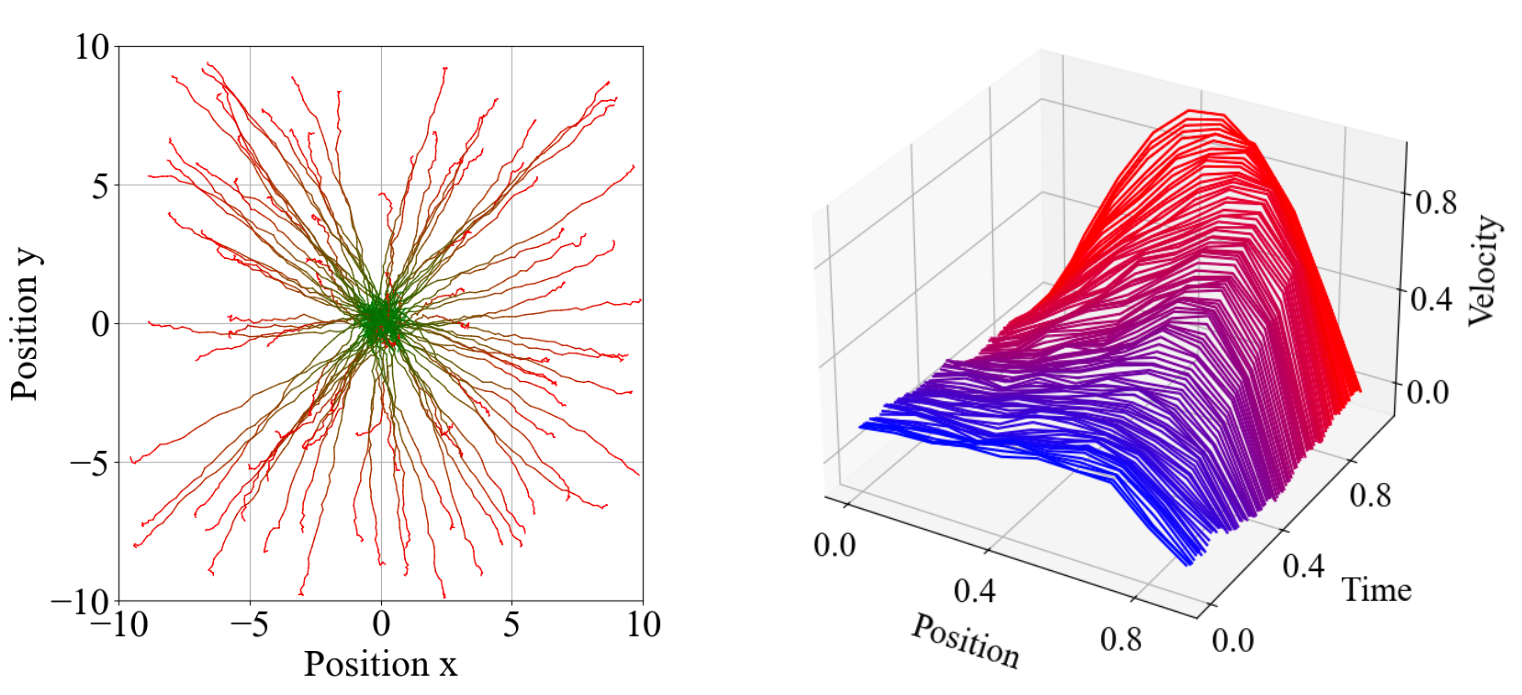
Figure 1: Navigation trajectories of an agent (Left) and velocity profile of the fluid over time (Right).

Navigation Problem. An agent moves in a horizontal plane following some linearized dynamics that are characterized by the double integrator model with zero-mean Gaussian noise (Shimizu et al., 2020; Ma et al., 2022). We aim to drive the agent to the origin, but constraining its velocity. When the dynamics are known and the reward function linearly weights quadratic penalties on position and action, this problem is an instance of the constrained linear regulation problem (Scokaert and Rawlings, 1998), which is known to have closed-form solution. Hence, we can directly apply D-PGPD (6) and AD-PGPD (9) (See Appendix F.1). However, we consider the dynamics to be unknown, and we leverage our sample-based implementation of AD-PGPD. Furthermore, we use absolute value penalties instead of quadratic ones, as the latter can result in unstable behavior in sample-based scenarios (Engel and Babuška, 2014). Conventional methods do not solve this problem straightforwardly. We compare our sample-based AD-PGPD with PGDual, a dual method with linear function approximation (Zhao and You, 2021; Brunke et al., 2022). Figure 2 shows the value functions of the policy iterates generated by AD-PGPD and PGDual over $40,000$ iterations. The oscillations of AD-PGPD are damped over time, and it converges to a feasible solution with low variance in reward and utility, indicating a near-deterministic behavior without constraint violations. In contrast, PGDual exhibits large variance, indicating that the resultant policy violates the constraint. Despite this, the final primal return performance of PGDual is similar to that of AD-PGPD on average.

Fluid Velocity Control. We apply D-PGPD (6) to the control of the velocity of an incompressible Newtonian fluid described by the one-dimensional Burgers’ equation (Baker et al., 2000), a non-linear stochastic control problem. The velocity profile of the fluid $z$ varies in a one-dimensional space $x\in[0,1]$ and time $t\in[0,1]$, and the goal is to drive the velocity of the fluid towards $0$ via the control action $a$, e.g., injection of polymers. By discretizing Burgers’ equation, we have a non-linear system $s_{t+1}=B_{0}s_{t}+B_{1}a_{t}+B_{2}s_{t}^{2}+\omega_{t}$, where $s_{t}\in{\mathbb{R}}^{d}$ is the state, $s_{t}^{2}$ is the element-wise squared state vector, $a_{t}\in{\mathbb{R}}^{d}$ is the control input, and $B_{0}$, $B_{1}$, $B_{2}\in{\mathbb{R}}^{d\times d}$ are matrices representing the discretized spatial operators and non-linear terms (Borggaard and Zietsman, 2020). The details can be found in Appendix F. We consider a reward function that penalizes the state quadratically, and a budget constraint that limits the total control action. We compare our sample-based AD-PGPD with PGDual. Figure 3 shows the value functions of the policy iterates generated by AD-PGPD and PGDual over $10,000$ iterations. The results are consistent with those of the navigation problem. The AD-PGPD algorithm successfully mitigates oscillations and converges to a feasible solution with low return variance. In contrast, although PGDual achieves similar objective value, it does not dampens oscillations, as indicated by the variance of the solution. This implies that PGDual occasionally violates the constraint in the last iterate.

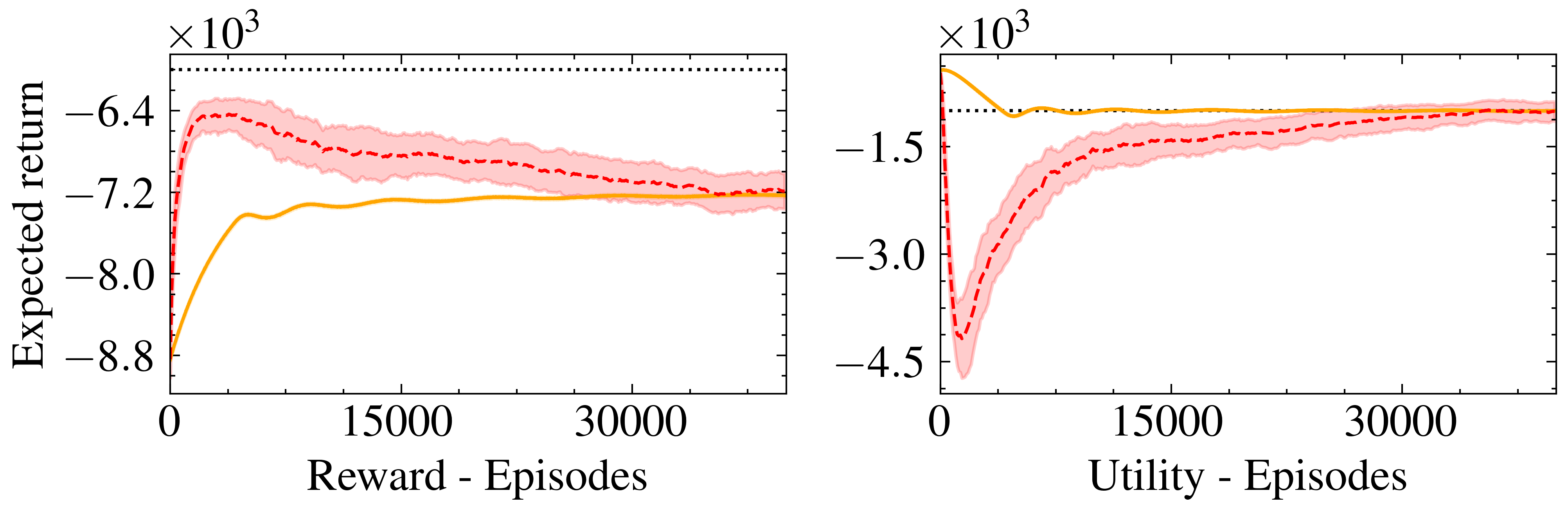
Figure 2: Average reward and utility value functions of policy iterates generated by AD-PGPD ( ) and PGDual (   ) in the navigation control problem with absolute-value rewards.

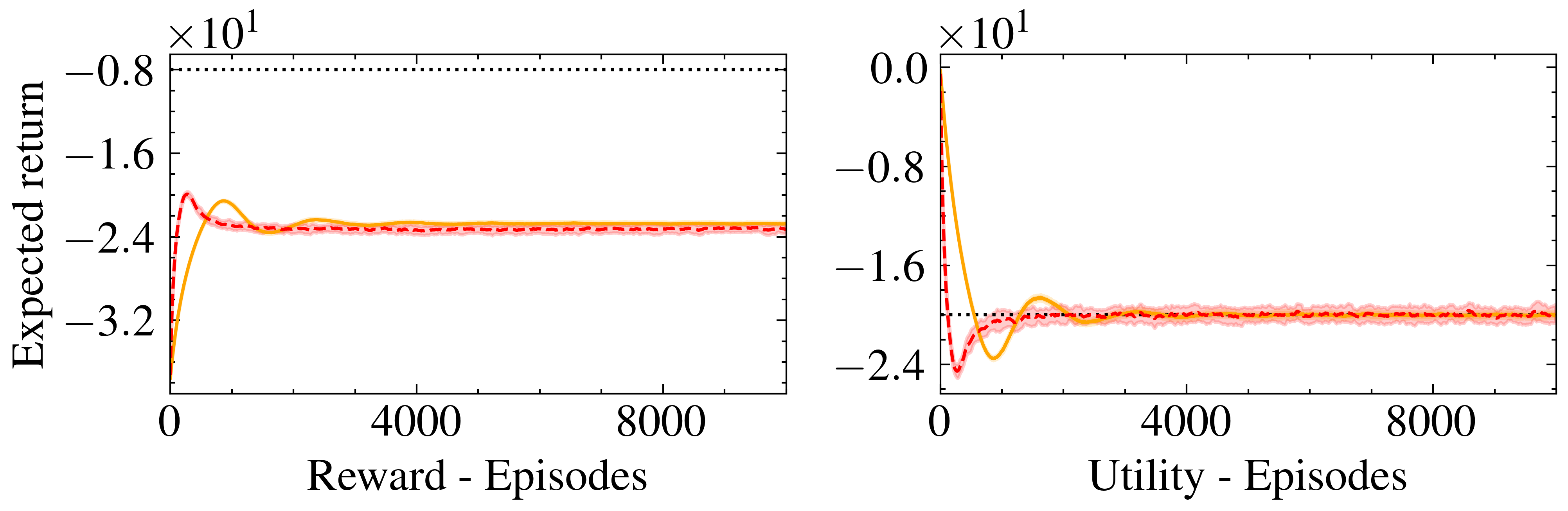
Figure 3: Average reward and utility value functions of policy iterates generated by AD-PGPD ( ) and PGDual (   ) in a fluid velocity control.

7 Concluding Remarks

We have presented a deterministic policy gradient primal-dual method for continuous state-action constrained MDPs with non-asymptotic convergence guarantees. We have leveraged function approximation to make the implementation practical and developed a sample-based algorithm. Furthermore, we have shown the effectiveness of the proposed method in a classical navigation problem and a non-linear fluid control problem under constraints. For future directions, our work stimulates many interesting problems on constrained MDPs with continuous state-action spaces: (i) minimal assumption on value functions; (ii) online exploration; (iii) optimal sample complexity; (iv) general function approximation.

Appendix A Convexity of Value Images

Strong duality holds for Problem (1), as established in Theorem 1, despite the non-convexity of the value functions $V_{r}(\pi)$ and $V_{g}(\pi)$ with respect to the policy $\pi$. This section aims to shed some light into the reasons behind this phenomenon. First, recall that the policy class $\Pi$ considered in this paper is restricted to deterministic policies. Importantly, this set is not necessarily convex. For any $\alpha\in[0,1]$ and two deterministic policies $\pi,\pi^{\prime}\in\Pi$, their convex combination

$$\pi_{\alpha}\;=\;\alpha\pi+(1-\alpha)\pi^{\prime},$$

does not generally yield to a deterministic policy, i.e., $\pi_{\alpha}\notin\Pi$. Furthermore, consider the vector value function

$$V(\pi)\;\mathrel{\mathop{:}}=\;\begin{bmatrix}V_{r}(\pi)\\[5.69046pt] V_{g}(\pi)\end{bmatrix}$$

associated with a given policy $\pi$. The value function $V(\pi)$ is non-convex in $\pi$. However, let us now focus on the set of all attainable vector value functions corresponding to deterministic policies, which defines the deterministic value image:

$$\mathcal{V}_{D}\;\mathrel{\mathop{:}}=\;\{V(\pi)\;|\;\pi\in\Pi\}.$$

Under the non-atomicity assumption (see Lemma 3), the set $\mathcal{V}_{D}$ is convex. This convexity implies that there exists a policy $\pi_{\alpha}\in\Pi$ such that

$$V(\pi_{\alpha})\;=\;\alpha V(\pi)+(1-\alpha)V(\pi^{\prime}),$$

even though $\pi_{\alpha}$ is not a convex combination of $\pi$ and $\pi^{\prime}$, and the vector value function $V$ remains non-convex.

Lastly, we consider the value image $\mathcal{V}_{T}$ for all policies. Under the non-atomicity assumption, these two sets, $\mathcal{V}_{D}$ and $\mathcal{V}_{T}$, are equivalent (see Lemma 4). Consequently, the optimal policy is contained within $\mathcal{V}_{D}$. Therefore, restricting the search space to deterministic policies is justified in the context of non-atomic MDPs. The convexity of the deterministic value image and its equivalence with the value image for all policies are illustrated in Figure 4.

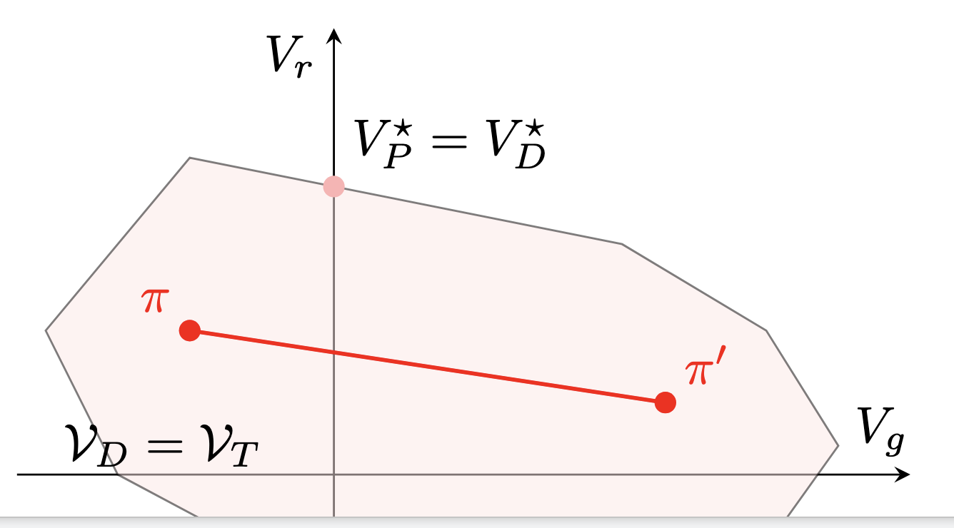
Figure 4: The deterministic value image ${\mathcal{V}}_{D}$ is convex and equivalent to the the value image for all policies: ${\mathcal{V}}_{T}$. Furthermore, constrained RL has zero duality gap in the deterministic policy space, i.e., $V_{P}^{\star}=V_{D}^{\star}$.

Appendix B Supporting Lemmas

Lemma 2 (Discounted and uniformly absorbing MDP equivalence).

A non-atomic discounted MDP can be equivalently represented as a non-atomic uniformly absorbing MDP.

Proof.

See Feinberg and Piunovskiy [2019, Lemma 3.12]. ∎

Lemma 3 (Convexity of the deterministic value image).

Consider the vector value function $V(\pi)\mathrel{\mathop{:}}=[V_{r}(\pi),V_{g}(\pi)]^{\top}$ for an arbitrary deterministic policy $\pi$. Let the span of value functions associated with the class of deterministic policies $\Pi$ be defined as ${\mathcal{V}}_{D}\mathrel{\mathop{:}}=\{V(\pi):\pi\in\Pi\}$.

Then, the set ${\mathcal{V}}_{D}$ is convex for a non-atomic uniformly absorbing MDP.

Proof.

See Feinberg and Piunovskiy [2019, Corollary 3.10]. ∎

Lemma 4 (Sufficiency of deterministic policies).

Consider the vector value function $V(\pi)\mathrel{\mathop{:}}=[V_{r}(\pi),V_{g}(\pi)]^{\top}$ for an arbitrary policy $\pi$. Let the span of value functions associated with the class of deterministic policies $\Pi$ be defined as ${\mathcal{V}}_{D}\mathrel{\mathop{:}}=\{V(\pi):\pi\in\Pi\}$. Similarly, let the span of value functions associated with the general class of policies $\Pi_{T}$ be defined as ${\mathcal{V}}_{T}\mathrel{\mathop{:}}=\{V(\pi)$ : $\pi\in\Pi_{T}\}$.

Then, for a non-atomic uniformly absorbing MDP, it holds that ${\mathcal{V}}_{D}={\mathcal{V}}_{T}$.

Proof.

See Feinberg and Piunovskiy [2019, Theorem 3.8]. ∎

Lemma 5 (Quadratic growth Lemma).

Let $f$ be a $\mu$-strongly-concave function and let $x^{\star}$ denote its maximizer. Then

$$f(x)\;\leq\;f(x^{\star})-\mu||x-x^{\star}||^{2}.$$ (14)

Proof.

See Lan [2020, Lemma 3.5]. ∎

Lemma 6 (Standard descent Lemma).

Let $f$ be a convex differentiable function, and let $x^{\star}$ denote the minimizer of $f$. Consider the following sequence

$$x_{t+1}\;=\;x_{t}-\eta\nabla f(x_{t}),$$

where $\eta$ is an step-size. Then, the following bound holds

$$(x_{t}-x^{\star})\nabla f(x_{t})\;\leq\;\frac{1}{2\eta}\left((x_{t}-x^{\star})^{2}-(x_{t+1}-x^{\star})^{2}\right)+\eta^{2}\|\nabla f(x_{t})\|^{2}.$$ (15)

Proof.

See Zinkevich [2003, Theorem 1] ∎

Lemma 7 (Performance difference Lemma).

Consider the following regularized reward function $r_{\tau}(s_{t},a_{t})-\frac{\tau}{2}\|a_{t}\|^{2}$, and the associated value functions

$$V^{\pi}(s) \;=\;\mathbb{E}_{\pi}\left[\sum_{t=0}^{\infty}\gamma^{t}r_{\tau}(s_{t},a_{t})\;|\;s_{0}=s\right]$$

$$Q^{\pi}(s,a) \;=\;\mathbb{E}_{\pi}\left[\sum_{t=0}^{\infty}\gamma^{t}r_{\tau}(s_{t},a_{t})\;|\;s_{0}=s,a_{0}=a\right].$$

Consider the regularized advantage function $A^{\pi}(s,a)=Q^{\pi}(s,a)-V^{\pi}(s)-\frac{\tau}{2}\|a\|^{2}+\frac{\tau}{2}\pi(s)^{2}$. Let $\pi$ and $\pi^{\prime}$ be two feasible policies and $\rho$ be the initial state distribution. Then

$$V(\pi^{\prime})-V(\pi)\;=\;\frac{1}{1-\gamma}\mathbb{E}_{s\sim d_{\rho}^{\pi^{\prime}}}\left[A^{\pi}(s,\pi^{\prime}(s))\right].$$ (16)

Proof.

Leveraging the performance difference lemma of the regularized advantage (see [Lan, 2022, Lemma 2.1]), it follows that:

$$V(\pi^{\prime})-V(\pi) \;=\;\mathbb{E}_{s_{0}\sim\rho}[V^{\pi^{\prime}}(s_{0})-V^{\pi}(s_{0})]$$

$$\;=\;\frac{1}{1-\gamma}\mathbb{E}_{s_{0}\sim\rho}[\mathbb{E}_{s\sim d_{s_{0}}^{\pi^{\prime}}}[A^{\pi}(s,\pi^{\prime}(s))]]$$

$$\;=\;\frac{1}{1-\gamma}\mathbb{E}_{s\sim d_{\rho}^{\pi^{\prime}}}[A^{\pi}(s,\pi^{\prime}(s))].$$

∎

Lemma 8 (Fenchel-Moreau).

If Slater’s condition holds for (1) and its perturbation function $P(\delta)$ is concave on $\delta$, then (1) has zero duality gap.

Proof.

See Auslender and Teboulle [2006, Theorem 5.1.4, Proposition 5.3.2] ∎

Lemma 9 (Boundedness of $\lambda^{\star}$).

Let Assumption 2 hold. Then,

$$0\;\leq\;\lambda^{\star}\;\leq\;\frac{V_{r}(\pi^{\star})-V_{r}(\bar{\pi})}{\xi}.$$

Proof.

See Ding et al. [2022, Lemma 3]. Let $\Lambda_{a}\mathrel{\mathop{:}}=\{\lambda\geq 0\mid D(\lambda)\leq a\}$ be a sublevel set of the dual function for $a\in\mathbb{R}$. Thanks to Assumption 2, for any $\lambda\in\Lambda_{a}$

$$a\;\geq\;D(\lambda)\;\geq\;\left(V_{r}(\bar{\pi})+\lambda V_{g}(\bar{\pi})\right)\;\geq\;V_{r}(\bar{\pi})+\lambda\xi,$$

where $\bar{\pi}$ is a Slater point. Thus,

$$\lambda\;\leq\;\frac{a-V_{r}(\bar{\pi})}{\xi}.$$

If we take $a=V_{r}(\pi^{\star})=V_{D}^{\lambda^{\star}}$, then $\Lambda_{a}=\Lambda^{\star}$ which concludes the proof. ∎

Lemma 10 (Danskin’s Theorem).

Consider the function

$$F(x)\mathrel{\mathop{:}}=\text{sup}_{y\,\in\,Y}f(x,y),$$ (17)

where $f$: ${\mathbb{R}}^{n}\times Y\to{\mathbb{R}}\cup\{-\infty,+\infty\}$. If the following conditions are satisfied,

1. The function $f(\cdot,y)$ is convex for all $y\in Y$;

2. The function $f(x,\cdot)$ is upper semicontinuous for all $x$ in a certain neighborhood of a point $x_{0}$;

3. The set $Y\subset{\mathbb{R}}^{m}$ is compact;

then, $F$ is a convex function w.r.t. $x$, and

$$\partial F(x_{0})\;=\;\text{conv}\left(\underset{y\,\in\,\hat{Y}(x_{0})}{\cup}\partial_{x}f(x_{0},y)\right)$$ (18)

where $\partial_{x}f(x_{0},y)$ denotes the subdifferential of the function $f(\cdot,y)$ at $x_{0}$, and $\hat{Y}(x_{0})$ denote the set of maximizing points of $F$ at $x_{0}$.

Proof.

See Ruszczyński [2006][Theorem 2.87]. ∎

Lemma 11.

(Lipschitz bound Lemma). Let Assumption 4 hold, and let $A_{\lambda,\tau}^{\pi}(s,a)=Q_{\lambda,\tau}^{\pi}(s,a)-V_{\lambda,\tau}^{\pi}(s)-\frac{\tau}{2}\|a\|^{2}+\frac{\tau}{2}\|\pi(s)\|^{2}$ and $\eta>0$. Then, it follows that

$$A_{\lambda,\tau}^{\pi}(s,a)-\frac{1}{2\eta}\|\pi(s)-a\|^{2}\;\leq\;\frac{\eta}{2}C_{P}^{2},$$ (19)

where $C_{P}\mathrel{\mathop{:}}=L_{r}+\lambda_{\text{max}}L_{g}+\tau L_{h}+\tau\sqrt{d_{a}}A_{\text{max}}$.

Proof.

The proof begins by manipulating the advantage using the fact that $V_{\lambda,\tau}^{\pi}(s)=Q_{\lambda,\tau}^{\pi}(s,\pi(s))$ for deterministic policies

$$A_{\lambda,\tau}^{\pi}(s,a)\;=\;\underbrace{Q_{\lambda,\tau}^{\pi}(s,a)-Q_{\lambda,\tau}^{\pi}(s,\pi(s))}_{\text{(i)}}-\underbrace{\frac{\tau}{2}\|a\|^{2}+\frac{\tau}{2}\|\pi(s)\|^{2}}_{\text{(ii)}}.$$

Now, we manipulate (i) leveraging the Lipschitz continuity assumption 4.

$$Q_{\lambda,\tau}^{\pi}(s,a)-Q_{\lambda,\tau}^{\pi}(s,\pi(s))$$ (20)

$$=\;\left(Q_{r}^{\pi}(s,a)-Q_{r}^{\pi}(s,\pi(s))\right)+\lambda\left(Q_{g}^{\pi}(s,a)-Q_{g}^{\pi}(s,\pi(s))\right)+\frac{\tau}{2}\left(H^{\pi}(s,a)-H^{\pi}(s,\pi(s))\right)$$

$$\leq\;\left(L_{r}+\lambda_{\text{max}}L_{g}+\tau L_{h}\right)\|\pi(s)-a\|.$$

For the term (ii), we have first that $\|\pi(s)\|^{2}-\|a\|^{2}$ is a difference of quadratics, so we can use it in combination with the triangular inequality to show that

$$\frac{\tau}{2}\|a\|^{2}+\frac{\tau}{2}\|\pi(s)\|^{2} \;=\;\frac{\tau}{2}(\pi(s)-a)^{\top}(\pi(s)+a)$$

$$\;\leq\;\frac{\tau}{2}\|\pi(s)-a\|\|\pi(s)+a\|.$$

Then, using the boundedness of the actions as $\|\pi(s)+a\|\leq 2\sqrt{d_{a}}A_{\text{max}}$, where $d_{a}$ is the dimensionality of $A$, we have that

$$\frac{\tau}{2}\|\pi(s)-a\|\times\|\pi(s)+a\|\;\leq\;\tau\sqrt{d_{a}}A_{\text{max}}\|\pi(s)-a\|.$$ (21)

Now, combining (20) and (21) we have that

$$A_{\lambda,\tau}^{\pi}(s,a)\;\leq\;\left(L_{r}+\lambda_{\text{max}}L_{g}+\tau L_{h}+\tau\sqrt{d_{a}}A_{\text{max}}\right)\|\pi(s)-a\|.$$ (22)

Now, we define $C_{P}\mathrel{\mathop{:}}=L_{r}+\lambda_{\text{max}}L_{g}+\tau L_{h}+\tau\sqrt{d_{a}}A_{\text{max}}$ and using (22) we have that

$$A_{\lambda,\tau}^{\pi}(s,a)-\frac{1}{2\eta}\|\pi(s)-a\|^{2}\;\leq\;C_{P}\|\pi(s)-a\|-\frac{1}{2\eta}\|\pi(s)-a\|^{2}.$$

We add and substract the term $\frac{\eta}{2}C_{P}^{2}$, to then complete the squares to show that

$$C_{P}\|\pi(s)-a\|-\frac{1}{2\eta}\|\pi(s)-a\|^{2}$$

$$=\;C_{P}\|\pi(s)-a\|-\frac{1}{2\eta}\|\pi(s)-a\|^{2}-\frac{\eta}{2}C_{P}^{2}+\frac{\eta}{2}C_{P}^{2}$$

$$=\;\frac{\eta}{2}C_{P}^{2}-\left(\frac{1}{\sqrt{2\eta}}\|\pi(s)-a\|-\frac{\sqrt{2\eta}}{2}C_{P}\right)^{2}.$$

Therefore, dropping the negative quadratic term we have that

$$A_{\lambda,\tau}^{\pi}(s,a)-\frac{1}{2\eta}\|\pi(s)-a\|^{2} \;=\;\frac{\eta}{2}C_{P}^{2}-\left(\frac{1}{\sqrt{2\eta}}\|\pi(s)-a\|-\frac{\sqrt{2\eta}}{2}C_{P}\right)^{2}$$

$$\;\leq\;\frac{\eta}{2}C_{P}^{2}$$

which concludes the proof. ∎

Lemma 12.

(Error bound lemma). For an arbitrary deterministic policy $\pi$, the expected approximation error $\delta(s,\pi(s))$ satisfies

$$\mathbb{E}_{s\sim d_{\rho}^{\star}}\left[\|\delta(s,\pi(s))\|\right]\;\leq\;(2A_{\text{max}})^{d_{a}}\mathbb{E}_{s\sim d_{\rho}^{\star},a\sim\mathsf{u}}\left[\|\delta(s,a)\|\right].$$ (23)

where $d_{\rho}^{\star}$ denotes the optimal state-visitation frequency, and $\mathsf{u}$ denotes the uniform distribution.

Proof.

Consider the multi-dimensional uniform distribution over the bounded action space $A\in[-A_{\text{max}},A_{\text{max}}]^{d_{a}}$. The probability density is given by the expression

$$u(a)\;\mathrel{\mathop{:}}=\;\begin{cases}\frac{1}{(2A_{\text{max}})^{d_{a}}}&\text{if}\;\;a\in A\\ 0&\text{otherwise}.\end{cases}$$ (24)

The derivation of the bound of the expectation error begins by multiplying and dividing by the uniform distribution as

$$\mathbb{E}_{s\sim d_{\rho}^{\star}}\left[\|\delta(s,\pi(s))\|\right]\;=\;\mathbb{E}_{s\sim d_{\rho}^{\star}}\left[\frac{u(\pi(s))}{u(\pi(s))}\|\delta(s,\pi(s))\|\right].$$

Then, we have that for a generic measurable set $X$ and an element $x_{0}\in X$, the relation $f(x_{0})g(x_{0})\leq\int_{X}f(x)g(x)dx$ holds for a generic probability density function $f$ if the image of the random variable $g$ is positive. Thus, as $\|\delta(s,\pi(s))\|$ is a positive random variable, we have that

$$\mathbb{E}_{s\sim d_{\rho}^{\star}}\left[\frac{u(\pi(s))}{u(\pi(s))}\|\delta(s,\pi(s))\|\right]\;\leq\;\mathbb{E}_{s\sim d_{\rho}^{\star},a\sim u}\left[\frac{1}{u(\pi(s))}\|\delta(s,a)\|\right].$$

Finally, using the definition of the uniform density in (24) we conclude showing that

$$\mathbb{E}_{s\sim d_{\rho}^{\star}}\left[\|\delta(s,\pi(s))\|\right] \;\leq\;\mathbb{E}_{s\sim d_{\rho}^{\star},a\sim u}\left[\frac{1}{u(\pi(s))}\|\delta(s,a)\|\right]$$

$$\;=\;(2A_{\text{max}})^{d_{a}}\mathbb{E}_{s\sim d_{\rho}^{\star},a\sim u}\left[\|\delta(s,a)\|\right].$$

∎

Appendix C Proofs

C.1 Proof of Existence of Global Saddle Points

Lemma 13 (Existence of global saddle points).

There exists a primal-dual pair $(\pi_{\tau}^{\star},\lambda_{\tau}^{\star})\in\Pi\times\Lambda$ such that $L_{\tau}(\pi_{\tau}^{\star},\lambda)\geq L_{\tau}(\pi_{\tau}^{\star},\lambda_{\tau}^{\star})\geq L_{\tau}(\pi,\lambda_{\tau}^{\star})$. Furthermore, the following property holds for all $(\pi,\lambda)\in\Pi\times\Lambda$,

$$V_{\lambda_{\tau}^{\star},\tau}(\pi)+\frac{\tau}{2}H(\pi)\;\leq\;V_{\lambda_{\tau}^{\star},\tau}(\pi_{\tau}^{\star})\;\leq\;V_{\lambda,\tau}(\pi_{\tau}^{\star})+\frac{\tau}{2}\lambda^{2}.$$ (25)

Proof.

We know that the Lagrangian $L(\pi,\lambda)$ has global saddle points due to strong duality; see Theorem 1. We want to show that the regularized Lagrangian $L_{\tau}(\pi,\lambda)$ has global saddle points too. With that goal in mind, we consider the following regularized problem

$$\begin{array}[]{rl}\displaystyle\operatornamewithlimits{max}_{\pi\,\in\,\Pi}&\;\;V_{r}(\pi)\,+\,\frac{\tau}{2}H(\pi)\\[5.69046pt] \operatornamewithlimits{s.t.}&\;\;V_{g}(\pi)\;\geq\;0,\end{array}$$ (26)

where $H(\pi)$ is the regularizer introduced in Section 3. The term $V_{r}(\pi)+\frac{\tau}{2}H(\pi)$ can be redefined in terms of the regularized reward function $r_{\tau}(s,a)\mathrel{\mathop{:}}=r(s,a)-\frac{\tau}{2}h_{a}(a)$. This leads to a value function $V_{r_{\tau}}(\pi)$. As Theorem 1 does not require any Assumption in terms of the reward function, it follows that Problem (26) has zero duality gap too. This implies that its associated Lagrangian $\hat{L}_{\tau}(\pi,\lambda)\mathrel{\mathop{:}}=V_{r}(\pi)+\frac{\tau}{2}H(\pi)+\lambda V_{g}(\pi)$ has global saddle points.

It remains to be shown that adding the regularization of the Lagrangian multiplier preserves some global saddle points, i.e., $L_{\tau}(\pi,\lambda)=\hat{L}_{\tau}(\pi,\lambda)+\frac{\tau}{2}\lambda^{2}$ has global saddle points. We first consider the dual problem associated with $\hat{L}_{\tau}(\pi,\lambda)$

$$\operatornamewithlimits{min}_{\lambda\in\lambda}\;\operatornamewithlimits{max}_{\pi\in\Pi}\;V_{r}(\pi)+\frac{\tau}{2}H(\pi)+\lambda V_{g}(\pi).$$ (27)

The Lagrangian multiplier $\lambda^{\star}_{\tau}=0$ is always a solution to the dual Problem (27) due to complementary slackness. We denote by $\pi^{\star}_{\tau}$ a primal solution associated with $\lambda^{\star}_{\tau}$. If $V_{g}(\pi^{\star}_{\tau})$ is strictly feasible, i.e. $V_{g}(\pi^{\star}_{\tau})>0$, it follows that $\lambda^{\star}_{\tau}=0$ is the minimizer of the dual function. Otherwise, if $V_{g}(\pi^{\star}_{\tau})=0$ the dual function does not depend on $\lambda$, and we can select $\lambda^{\star}_{\tau}=0$ safely. Furthermore, the pair $(\pi^{\star}_{\tau},\lambda^{\star}_{\tau})$ satisfies for all $\pi\in\Pi$,

$$\hat{L}_{\tau}(\pi^{\star}_{\tau},\lambda^{\star}_{\tau})+\frac{\tau}{2}(\lambda^{\star}_{\tau})^{2}\;\geq\;\hat{L}_{\tau}(\pi,\lambda^{\star}_{\tau})+\frac{\tau}{2}(\lambda^{\star}_{\tau})^{2}.$$

Similarly, as the minimum element of the set $\Lambda$ is zero, it follows that for all $\lambda\in\Lambda$,

$$\hat{L}_{\tau}(\pi^{\star}_{\tau},\lambda^{\star}_{\tau})+\frac{\tau}{2}(\lambda^{\star}_{\tau})^{2}\;\leq\;\hat{L}_{\tau}(\pi^{\star}_{\tau},\lambda)+\frac{\tau}{2}(\lambda)^{2}.$$

This implies that the pair $(\pi^{\star}_{\tau},\lambda^{\star}_{\tau})$ is a global saddle point of $L_{\tau}(\pi,\lambda)$, as it satisfies for all $(\pi,\lambda)\in\Pi\times\Lambda$,

$$L_{\tau}(\pi,\lambda^{\star}_{\tau})\;\leq\;L_{\tau}(\pi^{\star}_{\tau},\lambda^{\star}_{\tau})\;\leq\;L_{\tau}(\pi^{\star}_{\tau},\lambda).$$

Moreover, the first inequality implies that for any $\pi\in\Pi$ we have

$$V_{\lambda_{\tau}^{\star}}(\pi_{\tau}^{\star})+\frac{\tau}{2}H(\pi_{\tau}^{\star})+\frac{\tau}{2}h(\lambda_{\tau}^{\star})\;\geq\;V_{\lambda_{\tau}^{\star}}(\pi)+\frac{\tau}{2}H(\pi)+\frac{\tau}{2}h(\lambda_{\tau}^{\star})$$

which leads to

$$V_{\lambda_{\tau}^{\star}}(\pi_{\tau}^{\star})\;\geq\;V_{\lambda_{\tau}^{\star}}(\pi)+\frac{\tau}{2}H(\pi).$$

The second inequality implies that for any $\lambda\in\Lambda$ we have

$$V_{\lambda}(\pi_{\tau}^{\star})+\frac{\tau}{2}H(\pi_{\tau}^{\star})+\frac{\tau}{2}h(\lambda)$$

$$\;\geq\;V_{\lambda_{\tau}^{\star}}(\pi_{\tau}^{\star})+\frac{\tau}{2}H(\pi_{\tau}^{\star})+\frac{\tau}{2}h(\lambda_{\tau}^{\star})$$

$$\;\geq\;V_{\lambda_{\tau}^{\star}}(\pi_{\tau}^{\star})+\frac{\tau}{2}H(\pi_{\tau}^{\star})$$

which leads to

$$V_{\lambda}(\pi_{\tau}^{\star})+\frac{\tau}{2}h(\lambda)\;\geq\;V_{\lambda_{\tau}^{\star}}(\pi_{\tau}^{\star}).$$

Combining both inequalities we have for all $(\pi,\lambda)\in\Pi\times\Lambda$,

$$V_{\lambda_{\tau}^{\star}}(\pi)+\frac{\tau}{2}H(\pi)\;\leq\;V_{\lambda_{\tau}^{\star}}(\pi_{\tau}^{\star})\;\leq\;V_{\lambda}(\pi_{\tau}^{\star})+\frac{\tau}{2}\lambda^{2}$$

which concludes the proof. ∎

C.2 Proof of Theorem 1

Proof.

To establish zero duality gap we consider the perturbed function of Problem (1). For any $\delta\in{\mathbb{R}}$, the perturbation function $P(\delta)$ associated with (1) is defined as follows

$$P(\delta)\;\mathrel{\mathop{:}}=\;\operatornamewithlimits{max}_{\pi\in\Pi} \;\;V_{r}(\pi)$$ (28)

$$\operatornamewithlimits{s.t.} \;\;V_{g}(\pi)\geq\delta.$$

The proof relies on Lemma 8, which states that if Slater’s condition holds for (1) and its perturbation function $P(\delta)$ is concave on $\delta$, then (1) has zero duality gap, even if the problem in (1) is non-convex. Therefore, we have to show that $P(\delta)$ is convex. More precisely, we need to establish that for a perturbation $\delta_{\alpha}\mathrel{\mathop{:}}=\alpha\delta+(1-\alpha)\delta^{\prime}$, where $\alpha\in[0,1]$, it holds that

$$P(\delta_{\alpha})\;\mathrel{\mathop{:}}=\;P(\alpha\delta+(1-\alpha)\delta)\;\geq\;\alpha P(\delta)+(1-\alpha)P(\delta^{\prime}).$$

Let $\pi$ and $\pi^{\prime}$ be the policies that achieve the maximum value of $P(\delta)$ for perturbations $\delta$ and $\delta^{\prime}$ respectively. This implies

$$V_{g}(\pi)\;\geq\;\delta\;\;\text{and}\;\;V_{g}(\pi^{\prime})\;\geq\;\delta^{\prime}.$$ (29)

Now, for a given policy $\pi$, we consider the vector value function $V(\pi)\mathrel{\mathop{:}}=[V_{r}(\pi),V_{g}(\pi)]^{\top}$. We define the deterministic value image as the span of value functions associated with the class of deterministic policies $\Pi$ as:

$${\mathcal{V}}_{D}\;\mathrel{\mathop{:}}=\;\{V(\pi):\pi\in\Pi\}.$$

The deterministic value image ${\mathcal{V}}_{D}$ is convex for non-atomic MDPs (see Feinberg and Piunovskiy [2019, Corollary 3.10]. This implies that there exists $\pi_{\alpha}\in\Pi$ such that $V({\pi_{\alpha}})\mathrel{\mathop{:}}=\alpha V(\pi)+(1-\alpha)V({\pi^{\prime}})$. More precisely:

$$V_{r}({\pi_{\alpha}})\;=\;\alpha V_{r}(\pi)+(1-\alpha)V_{r}(\pi^{\prime})$$ (30)

$$V_{g}({\pi_{\alpha}})\;=\;\alpha V_{g}(\pi)+(1-\alpha)V_{g}({\pi^{\prime}}).$$ (31)

It follows immediately that the objective of (28) is convex. Then, it only remains to be confirmed that $\pi_{\alpha}$ is feasible for the perturbation $\delta_{\alpha}$. We perform a convex combination of the inequalities in (29) to show that

$$\alpha V_{g}({\pi})+(1-\alpha)V_{g}({\pi^{\prime}})\;\geq\;\delta_{\alpha}$$

$$\text{ and }\;\;V_{g}({\pi_{\alpha}})\;\geq\;\delta_{\alpha}$$

which concludes the proof. ∎

C.3 Proof of Unique Saddle Point

Proof.

The regularized Lagrangian $L_{\tau}(\pi,\lambda)$ is a regular unconstrained MDP for a fixed $\lambda$. For all $\lambda$, if the reward function $r_{\lambda,\tau}$ is convex on $s$ and strictly concave on $a$, and the dynamics are linear, the resultant unconstrained MDP is guaranteed to have a unique maximizer $\pi_{\tau}^{\star}(\lambda)$ [Cruz-Suárez et al., 2004, Montes-de Oca et al., 2013]. Now, consider the regularized dual function

$$D_{\tau}(\lambda)\;=\;\lambda^{2}+\operatornamewithlimits{max}_{\pi\in\Pi}V_{\lambda,\tau}(\pi).$$ (32)

We know by Danskin’s Theorem (see Lemma 10) that (i) the function (32) is convex w.r.t $\lambda$, and (ii) the minimizer $\lambda^{\star}_{\tau}$ is unique if the Lagrangian maximizer $\pi_{\tau}^{\star}(\lambda)$ is unique for all $\lambda\in\Lambda$. Therefore, we can conclude uniqueness of the primal-dual optimal pair of $L_{\tau}(\pi,\lambda)$ under concavity of the reward function $r_{\lambda,\tau}$ and linearity of the dynamics. ∎

C.4 Proof of Theorem 2

Proof.

We set up the stage by introducing the constants that will be relevant throughout the proof. First, we have $C_{P}\mathrel{\mathop{:}}=L_{r}+\lambda_{\text{max}}L_{g}+\tau L_{h}+\tau\sqrt{d_{a}}A_{\text{max}}$, where $L_{r}$, $L_{g}$, and $L_{h}$ are the Lipschitz constants of action value functions introduced in Assumption 4, and $A_{\text{max}}$ is the maximum action of the bounded action space $A$. Then, we have $C_{D}\mathrel{\mathop{:}}=\frac{1}{1-\gamma}(1+\frac{\tau}{\xi})\geq V_{g}(\pi_{t})+\tau\lambda_{t}$, where $\xi$ comes from the feasibility Assumption 2.

We also recall that the operator ${\mathcal{P}}_{\Pi^{\star}_{\tau}}$ projects a policy onto the set of regularized optimal policies $\Pi^{\star}_{\tau}$ with state visitation distribution $d^{\star}_{\rho}$. For a given policy $\pi_{t}$, we denote $\pi^{\star}_{\tau,t}\mathrel{\mathop{:}}={\mathcal{P}}_{\Pi^{\star}_{\tau}}(\pi_{t})$. Similarly, the operator ${\mathcal{P}}_{\Lambda^{\star}_{\tau}}$ projects a Lagrangian multiplier onto the set of regularized optimal Lagrangian multipliers $\Lambda^{\star}_{\tau}$, and the projection is denoted as $\lambda^{\star}_{\tau,t}\mathrel{\mathop{:}}={\mathcal{P}}_{\Lambda^{\star}_{\tau}}(\lambda_{t})$.

We proceed by decomposing the primal-dual gap by adding and substracting $L_{\tau}(\pi_{t},\lambda_{t})$,

$$L_{\tau}(\pi^{\star}_{\tau,t},\lambda_{t})-L_{\tau}(\pi_{t},\lambda^{\star}_{\tau,t})$$

$$=\;\underbrace{L_{\tau}(\pi^{\star}_{\tau,t},\lambda_{t})-L_{\tau}(\pi_{t},\lambda_{t})}_{\text{(i)}}\,+\,\underbrace{L_{\tau}(\pi_{t},\lambda_{t})-L_{\tau}(\pi_{t},\lambda^{\star}_{\tau,t})}_{\text{(ii)}}.$$

Let’s define the distance function $D_{t}(\pi^{\star}_{\tau,t})=\mathbb{E}_{d^{\star}_{\rho}}\left[\|\pi^{\star}_{\tau,t}(s)-\pi_{t}(s)\|^{2}\right]$. Now, using the definition of the regularized Lagrangian and the performance difference Lemma 7, we can show that for term (i) we have that

$$L_{\tau}(\pi^{\star}_{\tau,t},\lambda_{t})-L_{\tau}(\pi_{t},\lambda_{t}) \;=\;V_{\lambda_{t},\tau}(\pi^{\star}_{\tau,t})-V_{\lambda_{t},\tau}({\pi_{t}})$$ (33)

$$\;=\;\frac{1}{1-\gamma}\mathbb{E}_{d^{\star}_{\rho}}\left[A^{\pi_{t}}_{\lambda_{t},\tau}(s,\pi^{\star}_{\tau,t}(s))\right].$$

Note that the objective function in (6a) is strongly concave w.r.t. $a$. Therefore, we can leverage the quadratic growth Lemma 5 with the function $f(a)\mathrel{\mathop{:}}=A^{\pi_{t}}_{\lambda_{t},\tau}(s,a)-\frac{1}{2\eta}\|\pi_{t}(s)-a\|^{2}$, and its the maximizer being $a^{\star}=\pi_{t+1}(s)$. By the optimality conditions of (6a) we have that

$$\mathbb{E}_{d^{\star}_{\rho}}\left[A^{\pi_{t}}_{\lambda_{t},\tau}(s,\pi^{\star}_{\tau,t}(s))\right] \;\leq\;\mathbb{E}_{d^{\star}_{\rho}}\left[A^{\pi_{t}}_{\lambda_{t},\tau}(s,\pi_{t+1}(s))-\frac{1}{2\eta}\|\pi_{t+1}(s)-\pi_{t}(s)\|^{2}\right]$$ (34)

$$\;\;\;\;\;\;+\mathbb{E}_{d^{\star}_{\rho}}\left[\frac{1}{2\eta}\|\pi^{\star}_{\tau,t}(s)-\pi_{t}(s)\|^{2}\right]$$

$$\;\;\;\;\;\;-\mathbb{E}_{d^{\star}_{\rho}}\left[\left(\frac{1+\eta(\tau-\tau_{0})}{2\eta}\right)\|\pi^{\star}_{\tau,t}(s)-\pi_{t+1}(s)\|^{2}\right].$$

Now, we can use Lemma 11 with $a=\pi_{t+1}(s)$ to bound the term

$$\mathbb{E}_{d^{\star}_{\rho}}\left[A^{\pi_{t}}_{\lambda_{t},\tau}(s,\pi_{t+1}(s))-\frac{1}{2\eta}\|\pi_{t+1}(s)-\pi_{t}(s)\|^{2}\right]\;\leq\;\frac{\eta}{2}C_{P}^{2}.$$ (35)

Combining the expressions in (33), (34) and (35) we have that for term (i) it holds that

$$L_{\tau}(\pi^{\star}_{\tau,t},\lambda_{t})-L_{\tau}(\pi_{t},\lambda_{t})\;\leq\;\frac{D_{t}(\pi^{\star}_{\tau,t})-(1+\eta(\tau-\tau_{0}))D_{t+1}(\pi^{\star}_{\tau,t})}{2\eta(1-\gamma)}+\frac{\eta}{2(1-\gamma)}C_{P}^{2}.$$

For the second term (ii) we use the definition of the regularized Lagrangian and the definition of the regularized value function to show that

$$L_{\tau}(\pi_{t},\lambda_{t})-L_{\tau}(\pi_{t},\lambda^{\star}_{\tau,t})$$ (36)

$$=\;V_{\lambda_{t},\tau}({\pi_{t}})-V_{\lambda^{\star}_{\tau,t},\tau}({\pi_{t}})+\frac{\tau}{2}(\lambda_{t})^{2}-\frac{\tau}{2}(\lambda^{\star}_{\tau,t})^{2}$$

$$=\;(\lambda_{t}-\lambda^{\star}_{\tau,t})V_{g}(\pi_{t})+\frac{\tau}{2}(\lambda_{t})^{2}-\frac{\tau}{2}(\lambda^{\star}_{\tau,t})^{2}.$$

Then, completing the squares we have that

$$(\lambda_{t}-\lambda^{\star}_{\tau,t})V_{g}(\pi_{t})+\frac{\tau}{2}(\lambda_{t})^{2}-\frac{\tau}{2}(\lambda^{\star}_{\tau,t})^{2}$$ (37)

$$=\;(\lambda_{t}-\lambda^{\star}_{\tau,t})(V_{g}(\pi_{t})+\tau\lambda_{t})-\frac{\tau}{2}\|\lambda^{\star}_{\tau,t}-\lambda_{t}\|^{2}.$$

We can now use the standard descent Lemma 6 to show that

$$(\lambda_{t}-\lambda^{\star}_{\tau,t})(V_{g}(\pi_{t})+\tau\lambda_{t})-\frac{\tau}{2}\|\lambda^{\star}_{\tau,t}-\lambda_{t}\|^{2}$$ (38)

$$\leq\;\frac{\|\lambda^{\star}_{\tau,t}-\lambda_{t}\|^{2}-\|\lambda^{\star}_{\tau,t}-\lambda_{t+1}\|^{2}}{2\eta}+\frac{1}{2}\eta C_{D}^{2}-\frac{\tau}{2}\|\lambda_{t}-\lambda^{\star}_{\tau,t}\|^{2}$$

$$=\;\frac{(1-\eta\tau)\|\lambda^{\star}_{\tau,t}-\lambda_{t}\|^{2}-\|\lambda^{\star}_{\tau,t}-\lambda_{t+1}\|^{2}}{2\eta}+\frac{1}{2}\eta C_{D}^{2},$$

where the last equality rearranges the term $\frac{\tau}{2}\|\lambda_{t}-\lambda^{\star}_{\tau,t}\|^{2}$ inside the fraction. Now, combining the expressions in (36), (37) and (38) we have that for term (ii) it holds that

$$L_{\tau}(\pi_{t},\lambda_{t})-L_{\tau}(\pi_{t},\lambda^{\star}_{\tau,t})\;=\;\frac{(1-\eta\tau)\|\lambda^{\star}_{\tau,t}-\lambda_{t}\|^{2}-\|\lambda^{\star}_{\tau,t}-\lambda_{t+1}\|^{2}}{2\eta}+\frac{1}{2}\eta C_{D}^{2}.$$

The next step is to combine (i) and (ii). We define $C_{0}\mathrel{\mathop{:}}=C_{P}+C_{D}$ and since the duality gap $L_{\tau}(\pi^{\star}_{\tau,t},\lambda_{t})-L_{\tau}(\pi_{t},\lambda^{\star}_{\tau,t})$ is positive and holds for any $(\pi_{\tau}^{\star},\lambda_{\tau}^{\star})\in\Pi^{\star}_{\tau}\times\Lambda^{\star}_{\tau}$, we have that

$$0 \;\leq\;\eta(1-\gamma)\left(L_{\tau}(\pi^{\star}_{\tau,t},\lambda_{t})-L_{\tau}(\pi_{t},\lambda^{\star}_{\tau,t})\right)$$

$$\;\leq\;\frac{1}{2}D_{t}(\pi^{\star}_{\tau,t})+\frac{1-\eta\tau}{2}\|\lambda^{\star}_{\tau,t}-\lambda_{t}\|^{2}$$

$$\;\;\;\;\;\;-\frac{1+\eta(\tau-\tau_{0})}{2}D_{t+1}(\pi^{\star}_{\tau,t})-\frac{1}{2}\|\lambda^{\star}_{\tau,t}-\lambda_{t+1}\|^{2}+\eta^{2}C_{0}^{2}.$$

Rearranging the expression above, it follows that

$$\frac{1+\eta(\tau-\tau_{0})}{2}D_{t+1}(\pi^{\star}_{\tau,t})+\frac{1}{2}\|\lambda^{\star}_{\tau,t}-\lambda_{t+1}\|^{2}$$

$$=\;(1+\eta(\tau-\tau_{0}))\left(\frac{1}{2}D_{t+1}(\pi^{\star}_{\tau,t})+\frac{1}{2(1+\eta(\tau-\tau_{0}))}\|\lambda^{\star}_{\tau,t}-\lambda_{t+1}\|^{2}\right)$$

$$\leq\;\frac{1}{2}D_{t}(\pi^{\star}_{\tau,t})+\frac{1-\eta\tau}{2}\|\lambda^{\star}_{\tau,t}-\lambda_{t}\|^{2}+\eta^{2}C_{0}^{2}$$

$$\leq\;\frac{1}{2}D_{t}(\pi^{\star}_{\tau,t})+\frac{1}{2(1+\eta(\tau-\tau_{0}))}\|\lambda^{\star}_{\tau,t}-\lambda_{t}\|^{2}+\eta^{2}C_{0}^{2},$$

where the last inequality follows from the fact that $\tau_{0}\in[0,\tau)$, and therefore $\frac{1-\eta\tau}{2}\leq\frac{1}{2(1+\eta(\tau-\tau_{0}))}$. Therefore, in summary we have that

$$(1+\eta(\tau-\tau_{0}))\left(\frac{1}{2}D_{t+1}(\pi^{\star}_{\tau,t})+\frac{1}{2(1+\eta(\tau-\tau_{0}))}\|\lambda^{\star}_{\tau,t}-\lambda_{t+1}\|^{2}\right)$$ (39)

$$\;\leq\;\frac{1}{2}D_{t}(\pi^{\star}_{\tau,t})+\frac{1}{2(1+\eta(\tau-\tau_{0}))}\|\lambda^{\star}_{\tau,t}-\lambda_{t}\|^{2}+\eta^{2}C_{0}^{2}.$$

Now, since $\pi_{\tau}^{\star}={\mathcal{P}}_{\Pi^{\star}_{\tau}}(\pi_{t})$ and $\lambda_{\tau}^{\star}={\mathcal{P}}_{\Lambda^{\star}_{\tau}}(\lambda_{t})$ are projections, it holds that

$$\frac{1+\eta(\tau-\tau_{0})}{2}D_{t+1}(\pi^{\star}_{\tau,t+1})+\frac{1}{2}\|\lambda^{\star}_{\tau,t+1}-\lambda_{t+1}\|^{2}$$

$$=\;\frac{1+\eta(\tau-\tau_{0})}{2}\mathbb{E}_{d^{\star}_{\rho}}\left[\|({\mathcal{P}}_{\Pi^{\star}_{\tau}}(\pi_{t+1}(s))-\pi_{t+1}(s)\|^{2}\right]+\frac{1}{2}\|{\mathcal{P}}_{\Lambda^{\star}_{\tau}}(\lambda_{t+1})-\lambda_{t+1}\|^{2}$$

$$\leq\;\frac{1+\eta(\tau-\tau_{0})}{2}\mathbb{E}_{d^{\star}_{\rho}}\left[\|({\mathcal{P}}_{\Pi^{\star}_{\tau}}(\pi_{t}(s))-\pi_{t+1}(s)\|^{2}\right]+\frac{1}{2}\|{\mathcal{P}}_{\Lambda^{\star}_{\tau}}(\lambda_{t})-\lambda_{t+1}\|^{2}$$

$$=\;\frac{1+\eta(\tau-\tau_{0})}{2}D_{t+1}(\pi^{\star}_{\tau,t})+\frac{1}{2}\|\lambda^{\star}_{\tau,t}-\lambda_{t+1}\|^{2}.$$

In summary, we have that

$$\frac{1+\eta(\tau-\tau_{0})}{2}D_{t+1}(\pi^{\star}_{\tau,t+1})+\frac{1}{2}\|\lambda^{\star}_{\tau,t+1}-\lambda_{t+1}\|^{2}$$ (40)

$$=\;\frac{1+\eta(\tau-\tau_{0})}{2}D_{t+1}(\pi^{\star}_{\tau,t})+\frac{1}{2}\|\lambda^{\star}_{\tau,t}-\lambda_{t+1}\|^{2}.$$

We define the potential function $\Phi_{t}\mathrel{\mathop{:}}=\frac{1}{2}D_{t}(\pi_{\tau,t}^{\star})+\frac{1}{2(1+\eta(\tau-\tau_{0}))}\|{\mathcal{P}}_{\Lambda^{\star}_{\tau}}(\lambda_{t})-\lambda_{t}\|^{2}$ and combine the inequalities (40) and (39) to show

$$(1+\eta(\tau-\tau_{0}))\Phi_{t+1}\;\leq\;\Phi_{t}+\eta^{2}C_{0}^{2}.$$ (41)

The next step is to expand (41) so that we have

$$\Phi_{t+1} \;\leq\;\frac{1}{1+\eta(\tau-\tau_{0})}\Phi_{t}+\eta^{2}C_{0}^{2}$$

$$\;\leq\;\left(\frac{1}{1+\eta(\tau-\tau_{0})}\right)^{2}\Phi_{t-1}+\left(\eta^{2}+\eta^{2}\left(\frac{1}{1+\eta(\tau-\tau_{0})}\right)\right)C_{0}^{2}.$$

If we keep expanding recursively we end up having

$$\Phi_{t+1} \;\leq\;\left(\frac{1}{1+\eta(\tau-\tau_{0})}\right)^{t}\Phi^{1}+\left(\eta^{2}\left(1+\left(\frac{1}{1+\eta(\tau-\tau_{0})}\right)+\ldots\right)\right)C_{0}^{2}.$$

Finally, using the definition of the exponential for the first term, and using the geometric series for the second one, we have that

$$\Phi_{t+1}\;\leq\;{\rm e}^{-\frac{\eta(\tau-\tau_{0})}{1+\eta(\tau-\tau_{0})}t}\Phi_{1}+\frac{\eta(1+\eta(\tau-\tau_{0}))}{\tau-\tau_{0}}C_{0}^{2}$$

which completes the proof. ∎

C.5 Proof of Corollary 1

Proof.

Due to Theorem (2), taking $\tau=O(\epsilon)+\tau_{0}$ and $\eta=O(\epsilon)$ leads to $\Phi_{t+1}=O(\epsilon)$ for any $t=\Omega(\frac{1}{\epsilon^{3}}\text{log}\frac{1}{\epsilon})$, where $\Omega$ encapsulates some problem-dependent constants. For some $t=\Omega(\frac{1}{\epsilon^{3}}\text{log}\frac{1}{\epsilon})$ the primal-dual iterate $(\pi_{t},\lambda_{t})$ satisfies $D_{t}(\pi^{\star}_{\tau,t})=O(\epsilon)$ and $\frac{1}{2(1+\eta(\tau-\tau_{0}))}\|\lambda^{\star}_{\tau,t}-\lambda_{t}\|^{2}=O(\epsilon)$. Now, adding and substracting $V_{r}({\pi^{\star}_{\tau,t}})$ we have

$$V_{r}({\pi^{\star}})-V_{r}({\pi_{t}})\;=\;\underbrace{V_{r}({\pi^{\star}})-V_{r}({\pi^{\star}_{\tau,t}})}_{\text{(i)}}\,+\,\underbrace{V_{r}({\pi^{\star}_{\tau,t}})-V_{r}({\pi_{t}})}_{\text{(ii)}}.$$

For the term (i) we can take $\pi=\pi^{\star}$ in (5) to show

$$V_{r}({\pi^{\star}})+\frac{\tau}{2}H(\pi^{\star})\;\leq\;V_{r}({\pi^{\star}_{\tau,t}})+\lambda_{\tau}^{\star}\left(V_{g}({\pi^{\star}_{\tau,t}})-V_{g}({\pi^{\star}})\right).$$

Then, taking $\lambda=0$ in (5) leads to $\lambda_{\tau}^{\star}V_{g}({\pi^{\star}_{\tau}})\leq 0$. Noticing that $\pi^{\star}$ feasible implies $V_{g}({\pi^{\star}})\geq 0$ we have

$$V_{r}({\pi^{\star}})-V_{r}({\pi^{\star}_{\tau,t}})\;\leq\;-\frac{\tau}{2}H(\pi^{\star}).$$ (42)

For the term (ii), by the performance difference Lemma in 7 with $\tau=0$ we have that

$$V_{r}({\pi^{\star}_{\tau,t}})-V_{r}({\pi_{t}})\;=\;\frac{1}{1-\gamma}\mathbb{E}_{d^{\star}_{\rho}}\left[Q_{r}^{\pi_{t}}(s,\pi^{\star}_{\tau,t}(s))-Q_{r}^{\pi_{t}}(s,\pi_{t}(s))\right].$$

Then, we have that by Assumption 4 the action-value function is $L_{r}$-Lipschitz

$$\frac{1}{1-\gamma}\mathbb{E}_{d^{\star}_{\rho}}\left[Q_{r}^{\pi_{t}}(s,\pi^{\star}_{\tau,t}(s))-Q_{r}^{\pi_{t}}(s,\pi_{t}(s))\right] \;\leq\;\frac{L_{r}}{1-\gamma}\mathbb{E}_{d^{\star}_{\rho}}\left[\|\pi^{\star}_{\tau,t}(s)-\pi_{t}(s)\|\right]$$

$$\;=\;\frac{L_{r}}{1-\gamma}\mathbb{E}_{d^{\star}_{\rho}}\left[\sqrt{\|\pi^{\star}_{\tau,t}(s)-\pi_{t}(s)\|^{2}}\;\right],$$

where we have taken the square and the square root in the last equality. Note now that we can use Cauchy-Schwartz to show that

$$V_{r}({\pi^{\star}_{\tau,t}})-V_{r}({\pi_{t}}) \;=\;\frac{L_{r}}{1-\gamma}\mathbb{E}_{d^{\star}_{\rho}}\left[\sqrt{\|\pi^{\star}_{\tau,t}(s)-\pi_{t}(s)\|^{2}}\;\right]$$

$$\;\leq\;\frac{L_{r}}{1-\gamma}\sqrt{\mathbb{E}_{d^{\star}_{\rho}}\left[\|\pi^{\star}_{\tau,t}(s)-\pi_{t}(s)\|^{2}\right]}$$

$$\;=\;\frac{L_{r}}{1-\gamma}\sqrt{D_{t}(\pi^{\star}_{\tau,t})}.$$

Therefore, combining (i) and (ii) leads to $V_{r}({\pi^{\star}})-V_{r}({\pi_{t}})\leq O(\sqrt{\epsilon})-\frac{\tau_{0}}{2}H(\pi^{\star})$.

Then, for any $\pi^{\star}_{\tau}\in\Pi^{\star}_{\tau}$, we have

$$-V_{g}({\pi_{t}})\;=\;\underbrace{-V_{g}({\pi^{\star}_{\tau}})}_{\text{(iii)}}\,+\,\underbrace{V_{g}({\pi^{\star}_{\tau}})-V_{g}({\pi_{t}})}_{\text{(iv)}}.$$

For (iii) we take $\lambda=\lambda_{\text{max}}\mathrel{\mathop{:}}=\frac{1}{(1-\gamma)\xi}$ in (5) to show that $-(\lambda_{\text{max}}-\lambda_{\tau}^{\star})V_{g}({\pi_{\tau}^{\star}})\leq\frac{\tau}{2}(\lambda_{\text{max}})^{2}$. By the definition

$$\lambda_{\tau}^{\star}\;\mathrel{\mathop{:}}=\;\operatornamewithlimits{argmin}_{\lambda\in\Lambda}\;\lambda V_{g}({\pi_{\tau,t}^{\star}})+\frac{\tau}{2}\lambda^{2},$$

$\lambda_{\tau}^{\star}$ can take three different values:

1. When $0\leq-V_{g}({\pi_{\tau}^{\star}})/\tau\leq\lambda_{\text{max}}$, then $\lambda_{\tau}^{\star}=-V_{g}({\pi_{\tau}^{\star}})/\tau$ and $\lambda_{\text{max}}-\lambda_{\tau}^{\star}\geq 0$.

2. When $-V_{g}({\pi_{\tau}^{\star}})/\tau\leq 0$, then $\lambda_{\tau}^{\star}=0$ and $\lambda_{\text{max}}-\lambda_{\tau}^{\star}\geq 0$.

3. When $-V_{g}({\pi_{\tau}^{\star}})/\tau\geq\lambda_{\text{max}}$, then $\lambda_{\tau}^{\star}=\lambda_{\text{max}}$.

For the third case, we take $\pi=\pi^{\star}$ in (5) to show

$$\lambda_{\text{max}}(V_{g}({\pi^{\star}})-V_{g}({\pi^{\star}_{\tau}}))\;\leq\;V_{r}({\pi^{\star}_{\tau}})-V_{r}({\pi^{\star}})-\frac{\tau}{2}H(\pi^{\star}).$$ (43)

Furthermore, for any global saddle point of the non-regularized Lagrangian $(\pi^{\star},\lambda^{\star})\in\Pi^{\star}\times\Lambda^{\star}$, it holds

$$V_{r}({\pi^{\star}_{\tau}})-V_{r}({\pi^{\star}})\;\leq\;\lambda^{\star}(V_{g}({\pi^{\star}})-V_{g}({\pi^{\star}_{\tau}})).$$ (44)

Combining (43) and (44), and leveraging that $V_{g}(\pi^{\star})\geq 0$, we have

$$-(\lambda_{\text{max}}-\lambda^{\star})V_{g}({\pi^{\star}_{\tau}})\;\leq\;-\frac{\tau}{2}H(\pi^{\star}).$$

As $\lambda^{\star}\leq\lambda_{\text{max}}$ is a global saddle point, we can conclude that

$$-V_{g}({\pi_{\tau}^{\star}})\;\leq\;-\frac{\tau}{2(\lambda_{\text{max}}-\lambda^{\star})}H(\pi^{\star}).$$

The term (iv) has a similar bound to (ii), so we can show that it is $O(\sqrt{\epsilon})$. Combining (iii) and (iv) we have $-V_{g}({\pi_{t}})\leq O(\sqrt{\epsilon})-\frac{\tau_{0}}{2(\lambda_{\text{max}}-\lambda^{\star})}H(\pi^{\star})$. We replace $\sqrt{\epsilon}$ for $\epsilon$ and combine all big O notation to conclude the proof. ∎

C.6 Proof of Theorem 3

Proof.

We recall the constants that will be relevant throughout the proof. First, we have $C_{P}\mathrel{\mathop{:}}=L_{r}+\lambda_{\text{max}}L_{g}+\tau L_{h}+\tau\sqrt{d_{a}}A_{\text{max}}$, where $L_{r}$, $L_{g}$, and $L_{h}$ are the Lipschitz constants of action value functions introduced in Assumption 4, and $A_{\text{max}}$ is the maximum action of the bounded action space $A$. Then, we have $C_{D}\mathrel{\mathop{:}}=\frac{1}{1-\gamma}(1+\frac{\tau}{\xi})\geq V_{g}(\pi_{t})+\tau\lambda_{t}$, where $\xi$ comes from the feasibility Assumption 2. We also introduce again the operator ${\mathcal{P}}_{\Pi^{\star}_{\tau}}$ that projects a policy onto the set of regularized optimal policies $\Pi^{\star}_{\tau}$ with state visitation distribution $d^{\star}_{\rho}$. For a given policy $\pi_{t}$, we denote $\pi^{\star}_{\tau,t}\mathrel{\mathop{:}}={\mathcal{P}}_{\Pi^{\star}_{\tau}}(\pi_{t})$. Similarly, the operator ${\mathcal{P}}_{\Lambda^{\star}_{\tau}}$ projects a Lagrangian multiplier onto the set of regularized optimal Lagrangian multipliers $\Lambda^{\star}_{\tau}$, and the projection is denoted as $\lambda^{\star}_{\tau,t}\mathrel{\mathop{:}}={\mathcal{P}}_{\Lambda^{\star}_{\tau}}(\lambda_{t})$.

We begin by using the definition of the regularized advantage evaluated in $\pi^{\star}_{\tau,t}(s)$, and we add and substract $\frac{1}{\eta}\pi_{t}(s)^{\top}\pi^{\star}_{\tau,t}(s)$ so that we have

$$A_{\lambda_{t},\tau}^{\pi_{t}}(s,\pi^{\star}_{\tau,t}(s)) \;=\;Q_{\lambda_{t},\tau}^{\pi_{t}}(s,\pi^{\star}_{\tau,t}(s))-V_{\lambda_{t},\tau}^{\pi_{t}}(s)-\frac{\tau}{2}\|\pi^{\star}_{\tau,t}(s)\|^{2}+\frac{\tau}{2}\|\pi_{t}(s)\|^{2}$$

$$\;=\;Q_{\lambda_{t},\tau}^{\pi_{t}}(s,\pi^{\star}_{\tau,t}(s))-V_{\lambda_{t},\tau}^{\pi_{t}}(s)-\frac{\tau}{2}\|\pi^{\star}_{\tau,t}(s)\|^{2}$$

$$\;\;\;\;\;\;\;+\frac{\tau}{2}\|\pi_{t}(s)\|^{2}+\frac{1}{\eta}\pi_{t}(s)^{\top}\pi^{\star}_{\tau,t}(s)-\frac{1}{\eta}\pi_{t}(s)^{\top}\pi^{\star}_{\tau,t}(s).$$

Note that we can equivalently use the augmented action value function $J^{\pi_{t}}$ such that it holds that

$$A_{\lambda_{t},\tau}^{\pi_{t}}(s,\pi^{\star}_{\tau,t}(s)) \;=\;J^{\pi_{t}}(s,\pi^{\star}_{\tau,t}(s))-\frac{1}{\eta}\pi_{t}(s)^{\top}\pi^{\star}_{\tau,t}(s)-V_{\lambda_{t},\tau}^{\pi_{t}}(s)-\frac{\tau}{2}\|\pi^{\star}_{\tau,t}(s)\|^{2}+\frac{\tau}{2}\|\pi_{t}(s)\|^{2}.$$

Using the definition of the approximation error introduced in Assumption 6, $\delta_{\theta_{t}}(s,a)\mathrel{\mathop{:}}=\tilde{J}_{\theta_{t}}(s,a)-J^{\pi_{t}}(s,a)$, we have that

$$A_{\lambda_{t},\tau}^{\pi_{t}}(s,\pi^{\star}_{\tau,t}(s)) \;=\;\tilde{J}_{\theta_{t}}(s,\pi^{\star}_{\tau,t}(s))-\delta_{\theta_{t}}(s,\pi^{\star}_{\tau,t}(s))-\frac{1}{\eta}\pi_{t}(s)^{\top}\pi^{\star}_{\tau,t}(s)$$

$$\;\;\;\;\;-V_{\lambda_{t},\tau}^{\pi_{t}}(s)-\frac{\tau}{2}\|\pi^{\star}_{\tau,t}(s)\|^{2}+\frac{\tau}{2}\|\pi_{t}(s)\|^{2}.$$

Now, we can use the quadratic growth Lemma 5 and the optimality conditions of the strongly concave objective in (9a), with $f(a)=\tilde{J}_{\theta_{t}}(s,a)-\frac{\tau}{2}\|a\|^{2}-\frac{1}{2\eta}\|a\|^{2}$ and the maximizer being $a^{\star}=\pi_{t+1}(s)$ to show that the following bound holds

$$A_{\lambda_{t},\tau}^{\pi_{t}}(s,\pi^{\star}_{\tau,t}(s)) \;=\;\tilde{J}_{\theta_{t}}(s,\pi^{\star}_{\tau,t}(s))-\delta_{\theta_{t}}(s,\pi^{\star}_{\tau,t}(s))-\frac{1}{\eta}\pi_{t}(s)^{\top}\pi^{\star}_{\tau,t}(s)$$ (45)

$$\;\;\;\;\;\;-V_{\lambda_{t},\tau}^{\pi_{t}}(s)-\frac{\tau}{2}\|\pi^{\star}_{\tau,t}(s)\|^{2}+\frac{\tau}{2}\|\pi_{t}(s)\|^{2}$$

$$\;\leq\;\tilde{J}_{\theta_{t}}(s,\pi_{t+1}(s))-\frac{\tau}{2}\|\pi_{t+1}(s)\|^{2}-\frac{1}{2\eta}\|\pi_{t+1}(s)\|^{2}$$

$$\;\;\;\;\;\;-\left(\frac{1+\eta(\tau-\tau_{0})}{2\eta}\right)\|\pi^{\star}_{\tau,t}(s)-\pi_{t+1}(s)\|^{2}$$

$$\;\;\;\;\;\;+\frac{\tau}{2}\|\pi^{\star}_{\tau,t}(s)\|^{2}+\frac{1}{2\eta}\|\pi^{\star}_{\tau,t}(s)\|^{2}-\delta_{\theta_{t}}(s,\pi^{\star}_{\tau,t}(s))$$

$$\;\;\;\;\;\;-\frac{1}{\eta}\pi_{t}(s)^{\top}\pi^{\star}_{\tau,t}(s)-V_{\lambda_{t},\tau}^{\pi_{t}}(s)-\frac{\tau}{2}\|\pi^{\star}_{\tau,t}(s)\|^{2}$$

$$\;\;\;\;\;\;+\frac{\tau}{2}\|\pi_{t}(s)\|^{2}.$$

Using again the definition of the approximation error introduced in Assumption 6, we know that $J^{\pi_{t}}(s,a)\mathrel{\mathop{:}}=\tilde{J}_{\theta_{t}}(s,a)-\delta_{\theta_{t}}(s,a)$. Then, adding and substracting $\frac{\tau}{2}\|\pi_{t}(s)\|^{2}$ we have the following equality

$$\tilde{J}_{\theta_{t}}(s,\pi_{t+1}(s))-\frac{\tau}{2}\|\pi_{t+1}(s)\|^{2}-\frac{1}{2\eta}\|\pi_{t+1}(s)\|^{2}-\left(\frac{1+\eta(\tau-\tau_{0})}{2\eta}\right)\|\pi^{\star}_{\tau,t}(s)-\pi_{t+1}(s)\|^{2}$$ (46)

$$+\frac{\tau}{2}\|\pi^{\star}_{\tau,t}(s)\|^{2}+\frac{1}{2\eta}\|\pi^{\star}_{\tau,t}(s)\|^{2}-\delta_{\theta_{t}}(s,\pi^{\star}_{\tau,t}(s))-\frac{1}{\eta}\pi_{t}(s)^{\top}\pi^{\star}_{\tau,t}(s)$$

$$-V_{\lambda_{t},\tau}^{\pi_{t}}(s)-\frac{\tau}{2}\|\pi^{\star}_{\tau,t}(s)\|^{2}+\frac{\tau}{2}\|\pi_{t}(s)\|^{2}$$

$$=\;J^{\pi_{t}}(s,\pi_{t+1}(s))+\delta_{\theta_{t}}(s,\pi_{t+1}(s))-\frac{\tau}{2}\|\pi_{t+1}(s)\|^{2}-\frac{1}{2\eta}\|\pi_{t+1}(s)\|^{2}$$

$$\;\;\;\;\;\;-\left(\frac{1+\eta(\tau-\tau_{0})}{2\eta}\right)\|\pi^{\star}_{\tau,t}(s)-\pi_{t+1}(s)\|^{2}+\frac{\tau}{2}\|\pi^{\star}_{\tau,t}(s)\|^{2}+\frac{1}{2\eta}\|\pi^{\star}_{\tau,t}(s)\|^{2}-\delta_{\theta_{t}}(s,\pi^{\star}_{\tau,t}(s))$$

$$\;\;\;\;\;\;-\frac{1}{\eta}\pi_{t}(s)^{\top}\pi^{\star}_{\tau,t}(s)-V_{\lambda_{t},\tau}^{\pi_{t}}(s)-\frac{\tau}{2}\|\pi^{\star}_{\tau,t}(s)\|^{2}+\frac{1}{2\eta}\|\pi_{t}(s)\|^{2}-\frac{1}{2\eta}\|\pi_{t}(s)\|^{2}+\frac{\tau}{2}\|\pi_{t}(s)\|^{2}.$$

We can rearrange some terms in the expression above by realizing that they are expanded differences of quadratics. Therefore, after some cumbersome algebraic manipulations we have that it holds that

$$J^{\pi_{t}}(s,\pi_{t+1}(s))+\delta_{\theta_{t}}(s,\pi_{t+1}(s))-\frac{\tau}{2}\|\pi_{t+1}(s)\|^{2}-\frac{1}{2\eta}\|\pi_{t+1}(s)\|^{2}$$ (47)

$$-\left(\frac{1+\eta(\tau-\tau_{0})}{2\eta}\right)\|\pi^{\star}_{\tau,t}(s)-\pi_{t+1}(s)\|^{2}+\frac{\tau}{2}\|\pi^{\star}_{\tau,t}(s)\|^{2}+\frac{1}{2\eta}\|\pi^{\star}_{\tau,t}(s)\|^{2}-\delta_{\theta_{t}}(s,\pi^{\star}_{\tau,t}(s))$$

$$-\frac{1}{\eta}\pi_{t}(s)^{\top}\pi^{\star}_{\tau,t}(s)-V_{\lambda_{t},\tau}^{\pi_{t}}(s)-\frac{\tau}{2}\|\pi^{\star}_{\tau,t}(s)\|^{2}+\frac{1}{2\eta}\|\pi_{t}(s)\|^{2}-\frac{1}{2\eta}\|\pi_{t}(s)\|^{2}+\frac{\tau}{2}\|\pi_{t}(s)\|^{2}$$

$$=\;A_{\lambda_{t},\tau}^{\pi_{t}}(s,\pi_{t+1}(s))-\frac{1}{2\eta}\|\pi_{t}(s)-\pi_{t+1}(s)\|^{2}+\frac{1}{2\eta}\|\pi^{\star}_{\tau,t}(s)-\pi_{t}(s)\|^{2}$$

$$\;\;\;\;\;\;-\left(\frac{1+\eta(\tau-\tau_{0})}{2\eta}\right)\|\pi^{\star}_{\tau,t}(s)-\pi_{t+1}(s)\|^{2}+\delta_{\theta_{t}}(s,\pi_{t+1}(s))-\delta_{\theta_{t}}(s,\pi^{\star}_{\tau,t}(s)).$$

In summary, combining the bounds in (45), (46), and (47) we have that

$$A_{\lambda_{t},\tau}^{\pi_{t}}(s,\pi^{\star}_{\tau,t}(a)) \;\leq\;A_{\lambda_{t},\tau}^{\pi_{t}}(s,\pi_{t+1}(s))-\frac{1}{2\eta}\|\pi_{t}(s)-\pi_{t+1}(s)\|^{2}+\frac{1}{2\eta}\|\pi^{\star}_{\tau,t}(s)-\pi_{t}(s)\|^{2}$$ (48)

$$\;\;\;\;\;\;-\left(\frac{1+\eta(\tau-\tau_{0})}{2\eta}\right)\|\pi^{\star}_{\tau,t}(s)-\pi_{t+1}(s)\|^{2}+\delta_{\theta_{t}}(s,\pi_{t+1}(s))-\delta_{\theta_{t}}(s,\pi^{\star}_{\tau,t}(s)).$$

With this bound in place, we can now decompose the primal-dual gap by adding and substracting $L_{\tau}(\pi_{t},\lambda_{t})$ as we did in the proof of Theorem (2) (see Corollary C.4)

$$L_{\tau}(\pi^{\star}_{\tau,t},\lambda_{t})-L_{\tau}(\pi_{t},\lambda^{\star}_{\tau,t})\;=\;\underbrace{L_{\tau}(\pi^{\star}_{\tau,t},\lambda_{t})-L_{\tau}(\pi_{t},\lambda_{t})}_{\text{(i)}}\,+\,\underbrace{L_{\tau}(\pi_{t},\lambda_{t})-L_{\tau}(\pi_{t},\lambda^{\star}_{\tau,t})}_{\text{(ii)}}.$$

Let’s define the distance function $D_{t}(\pi^{\star}_{\tau,t})=\mathbb{E}_{d^{\star}_{\rho}}\left[\|\pi^{\star}_{\tau,t}(s)-\pi_{t}(s)\|^{2}\right]$. Now, using the definition of the regularized Lagrangian and the performance difference Lemma 7, we can show that for term (i) we have that

$$L_{\tau}(\pi^{\star}_{\tau,t},\lambda_{t})-L_{\tau}(\pi_{t},\lambda_{t}) \;=\;V_{\lambda_{t},\tau}(\pi^{\star}_{\tau,t})-V_{\lambda_{t},\tau}({\pi_{t}})$$ (49)

$$\;=\;\frac{1}{1-\gamma}\mathbb{E}_{d^{\star}_{\rho}}\left[A^{\pi_{t}}_{\lambda_{t},\tau}(s,\pi^{\star}_{\tau,t}(s))\right].$$

Now, using the bound in (48) that we have just derive we have that

$$\mathbb{E}_{d^{\star}_{\rho}}\left[A^{\pi_{t}}_{\lambda_{t},\tau}(s,\pi^{\star}_{\tau,t}(s))\right] \;\leq\;\mathbb{E}_{d^{\star}_{\rho}}\left[A^{\pi_{t}}_{\lambda_{t},\tau}(s,\pi_{t+1}(s))-\frac{1}{2\eta}\|\pi_{t+1}(s)-\pi_{t}(s)\|^{2}\right]$$ (50)

$$\;\;\;\;\;\;+\mathbb{E}_{d^{\star}_{\rho}}\left[\frac{1}{2\eta}\|\pi^{\star}_{\tau,t}(s)-\pi_{t}(s)\|^{2}\right]$$

$$\;\;\;\;\;\;-\mathbb{E}_{d^{\star}_{\rho}}\left[\left(\frac{1+\eta(\tau-\tau_{0})}{2\eta}\right)\|\pi^{\star}_{\tau,t}(s)-\pi_{t+1}(s)\|^{2}\right]$$

$$\;\;\;\;\;\;+\mathbb{E}_{d^{\star}_{\rho}}\left[\delta_{\theta_{t}}(s,\pi_{t+1}(s))-\delta_{\theta_{t}}(s,\pi^{\star}_{\tau,t}(s))\right].$$

Also, we can use Lemma 12, Assumption 6 and the triangular inequality to establish that

$$\mathbb{E}_{d^{\star}_{\rho}}\left[\delta_{\theta_{t}}(s,\pi_{t+1}(s))-\delta_{\theta_{t}}(s,\pi^{\star}_{\tau,t}(s))\right] \;\leq\;2(2A_{\text{max}})^{d_{a}}\mathbb{E}_{s\sim d^{\star}_{\rho},a\sim\mathsf{u}}\left[\|\delta_{\theta_{t}}(s,a)\|\right]$$ (51)

$$\;\leq\;\epsilon_{\text{approx}},$$

where $\mathsf{u}$ is the uniform distribution. Furthermore, we can use Lemma 11 with $a=\pi_{t+1}(s)$ to bound the term

$$\mathbb{E}_{d^{\star}_{\rho}}\left[A^{\pi_{t}}_{\lambda_{t},\tau}(s,\pi_{t+1}(s))-\frac{1}{2\eta}\|\pi_{t+1}(s)-\pi_{t}(s)\|^{2}\right]\;\leq\;\frac{\eta}{2}C_{P}^{2}.$$ (52)

Finally, combining (49), (50), (51), and (52), we have that for the term (i) it holds that

$$L_{\tau}(\pi^{\star}_{\tau,t},\lambda_{t})-L_{\tau}(\pi_{t},\lambda_{t})$$

$$\leq\frac{D_{t}(\pi^{\star}_{\tau,t})-(1+\eta(\tau-\tau_{0}))D_{t+1}(\pi^{\star}_{\tau,t})}{2\eta(1-\gamma)}+\frac{\eta}{2(1-\gamma)}C_{P}^{2}+\frac{1}{1-\gamma}\epsilon_{\text{approx}}.$$

For the second term (ii) we use the definition of the regularized Lagrangian and the definition of the regularized value function to show that

$$L_{\tau}(\pi_{t},\lambda_{t})-L_{\tau}(\pi_{t},\lambda^{\star}_{\tau,t}) \;=\;V_{\lambda_{t},\tau}({\pi_{t}})-V_{\lambda^{\star}_{\tau,t},\tau}({\pi_{t}})+\frac{\tau}{2}(\lambda_{t})^{2}-\frac{\tau}{2}(\lambda^{\star}_{\tau,t})^{2}$$ (53)

$$\;=\;(\lambda_{t}-\lambda^{\star}_{\tau,t})V_{g}(\pi_{t})+\frac{\tau}{2}(\lambda_{t})^{2}-\frac{\tau}{2}(\lambda^{\star}_{\tau,t})^{2}.$$

Then, completing the squares we have that

$$(\lambda_{t}-\lambda^{\star}_{\tau,t})V_{g}(\pi_{t})+\frac{\tau}{2}(\lambda_{t})^{2}-\frac{\tau}{2}(\lambda^{\star}_{\tau,t})^{2}\;=\;(\lambda_{t}-\lambda^{\star}_{\tau,t})(V_{g}(\pi_{t})+\tau\lambda_{t})-\frac{\tau}{2}\|\lambda^{\star}_{\tau,t}-\lambda_{t}\|^{2}.$$ (54)

We can now use the standard descent Lemma 6 to show that

$$(\lambda_{t}-\lambda^{\star}_{\tau,t})(V_{g}(\pi_{t})+\tau\lambda_{t})-\frac{\tau}{2}\|\lambda^{\star}_{\tau,t}-\lambda_{t}\|^{2}$$ (55)

$$\leq\;\frac{\|\lambda^{\star}_{\tau,t}-\lambda_{t}\|^{2}-\|\lambda^{\star}_{\tau,t}-\lambda_{t+1}\|^{2}}{2\eta}+\frac{1}{2}\eta C_{D}^{2}-\frac{\tau}{2}\|\lambda_{t}-\lambda^{\star}_{\tau,t}\|^{2}$$

$$=\;\frac{(1-\eta\tau)\|\lambda^{\star}_{\tau,t}-\lambda_{t}\|^{2}-\|\lambda^{\star}_{\tau,t}-\lambda_{t+1}\|^{2}}{2\eta}+\frac{1}{2}\eta C_{D}^{2},$$

where the last equality rearranges the term $\frac{\tau}{2}\|\lambda_{t}-\lambda^{\star}_{\tau,t}\|^{2}$ inside the fraction. Now, combining the expressions in (53), (54) and (55) we have that for term (ii) it holds that

$$L_{\tau}(\pi_{t},\lambda_{t})-L_{\tau}(\pi_{t},\lambda^{\star}_{\tau,t})\;=\;\frac{(1-\eta\tau)\|\lambda^{\star}_{\tau,t}-\lambda_{t}\|^{2}-\|\lambda^{\star}_{\tau,t}-\lambda_{t+1}\|^{2}}{2\eta}+\frac{1}{2}\eta C_{D}^{2}.$$

We define $C_{0}\mathrel{\mathop{:}}=C_{P}+C_{D}$ and combine (i) and (ii) to show

$$0 \;\leq\;\eta(1-\gamma)\left(L_{\tau}(\pi^{\star}_{\tau,t},\lambda_{t})-L_{\tau}(\pi_{t},\lambda^{\star}_{\tau,t})\right)$$

$$\;\leq\;\frac{1}{2}D_{t}(\pi^{\star}_{\tau,t})+\frac{1-\eta\tau}{2}\|\lambda^{\star}_{\tau,t}-\lambda_{t}\|^{2}$$

$$\;\;\;\;\;\;-\frac{1+\eta(\tau-\tau_{0})}{2}D_{t+1}(\pi^{\star}_{\tau,t})-\frac{1}{2}\|\lambda^{\star}_{\tau,t}-\lambda_{t+1}\|^{2}+\eta^{2}C_{0}^{2}+\eta\epsilon_{\text{approx}},$$

where the first inequality follows from the fact that the duality gap is positive and holds for any $(\pi_{\tau}^{\star},\lambda_{\tau}^{\star})\in\Pi^{\star}_{\tau}\times\Lambda^{\star}_{\tau}$. Rearranging the expression above, it follows

$$\frac{1+\eta(\tau-\tau_{0})}{2}D_{t+1}(\pi^{\star}_{\tau,t})+\frac{1}{2}\|\lambda^{\star}_{\tau,t}-\lambda_{t+1}\|^{2}$$ (56)

$$=\;(1+\eta(\tau-\tau_{0}))\left(\frac{1}{2}D_{t+1}(\pi^{\star}_{\tau,t})+\frac{1}{2(1+\eta(\tau-\tau_{0}))}\|\lambda^{\star}_{\tau,t}-\lambda_{t+1}\|^{2}\right)$$

$$\leq\;\frac{1}{2}D_{t}(\pi^{\star}_{\tau,t})+\frac{1-\eta\tau}{2}\|\lambda^{\star}_{\tau,t}-\lambda_{t}\|^{2}+\eta^{2}C_{0}^{2}+\eta\epsilon_{\text{approx}}$$

$$\leq\;\frac{1}{2}D_{t}(\pi^{\star}_{\tau,t})+\frac{1}{2(1+\eta(\tau-\tau_{0}))}\|\lambda^{\star}_{\tau,t}-\lambda_{t}\|^{2}+\eta^{2}C_{0}^{2}+\eta\epsilon_{\text{approx}},$$

where the last inequality follows from the fact that $\tau_{0}\in[0,\tau)$, and therefore $\frac{1-\eta\tau}{2}\leq\frac{1}{2(1+\eta(\tau-\tau_{0}))}$. Since $\pi_{\tau}^{\star}={\mathcal{P}}_{\Pi^{\star}_{\tau}}(\pi_{t})$ and $\lambda_{\tau}^{\star}={\mathcal{P}}_{\Lambda^{\star}_{\tau}}(\lambda_{t})$ are projections, it holds that

$$\frac{1+\eta(\tau-\tau_{0})}{2}D_{t+1}(\pi^{\star}_{\tau,t+1})+\frac{1}{2}\|\lambda^{\star}_{\tau,t+1}-\lambda_{t+1}\|^{2}$$ (57)

$$=\;\frac{1+\eta(\tau-\tau_{0})}{2}\mathbb{E}_{d^{\star}_{\rho}}\left[\|({\mathcal{P}}_{\Pi^{\star}_{\tau}}(\pi_{t+1}(s))-\pi_{t+1}(s)\|^{2}\right]+\frac{1}{2}\|{\mathcal{P}}_{\Lambda^{\star}_{\tau}}(\lambda_{t+1})-\lambda_{t+1}\|^{2}$$

$$\leq\;\frac{1+\eta(\tau-\tau_{0})}{2}\mathbb{E}_{d^{\star}_{\rho}}\left[\|({\mathcal{P}}_{\Pi^{\star}_{\tau}}(\pi_{t}(s))-\pi_{t+1}(s)\|^{2}\right]+\frac{1}{2}\|{\mathcal{P}}_{\Lambda^{\star}_{\tau}}(\lambda_{t})-\lambda_{t+1}\|^{2}$$

$$=\;\frac{1+\eta(\tau-\tau_{0})}{2}D_{t+1}(\pi^{\star}_{\tau,t})+\frac{1}{2}\|\lambda^{\star}_{\tau,t}-\lambda_{t+1}\|^{2}.$$

We define the potential function $\Phi_{t}\mathrel{\mathop{:}}=\frac{1}{2}D_{t}(\pi_{\tau,t}^{\star})+\frac{1}{2(1+\eta(\tau-\tau_{0}))}\|{\mathcal{P}}_{\Lambda^{\star}_{\tau}}(\lambda_{t})-\lambda_{t}\|^{2}$, and combine the inequalities (57) and (56) to show

$$(1+\eta(\tau-\tau_{0}))\Phi_{t+1}\;\leq\;\Phi_{t}+\eta^{2}C_{0}^{2}+\eta\epsilon_{\text{approx}}.$$ (58)

The next step is to expand (58) so that we have

$$\Phi_{t+1} \;\leq\;\frac{1}{1+\eta(\tau-\tau_{0})}\Phi_{t}+\eta^{2}C_{0}^{2}+\eta\epsilon_{\text{approx}}$$

$$\;\leq\;\left(\frac{1}{1+\eta(\tau-\tau_{0})}\right)^{2}\Phi_{t-1}+\left(\eta^{2}+\eta^{2}\left(\frac{1}{1+\eta(\tau-\tau_{0})}\right)\right)\left(C_{0}^{2}+\frac{\epsilon_{\text{approx}}}{\eta}\right).$$

If we keep expanding recursively we end up having

$$\Phi_{t+1} \;\leq\;\left(\frac{1}{1+\eta(\tau-\tau_{0})}\right)^{t}\Phi^{1}+\left(\eta^{2}\left(1+\left(\frac{1}{1+\eta(\tau-\tau_{0})}\right)+\ldots\right)\right)\left(C_{0}^{2}+\frac{\epsilon_{\text{approx}}}{\eta}\right).$$

Finally, using the definition of the exponential for the first term, and using the geometric series for the second one, we have that

$$\Phi_{t+1}\leq{\rm e}^{-\frac{\eta(\tau-\tau_{0})}{1+\eta(\tau-\tau_{0})}t}\Phi_{1}+\frac{\eta(1+\eta(\tau-\tau_{0}))}{\tau-\tau_{0}}C_{0}^{2}+\frac{1+\eta(\tau-\tau_{0})}{\tau-\tau_{0}}\epsilon_{\text{approx}}$$

which completes the proof.

∎

C.7 Proof of Corollary 3

Proof.

The proof is an extension of the proof of Theorem 3. However, we need to take into account the randomness of estimating $\theta_{t}$ using samples. As the updates in (12) are performed using projected SGD, we can leverage known error bounds Lacoste-Julien et al. [2012] to bound the expected estimation error

$$\delta(\theta_{t},\hat{\theta}_{t},\nu)\mathrel{\mathop{:}}=\mathbb{E}_{\nu}\left[\delta_{\theta_{t}^{(n)}}(s,a)-\delta_{\theta_{t}}(s,a)\right].$$

With that goal in mind, we need to check:

1. The domain $\|\theta\|\leq\theta_{\text{max}}$ is convex and bounded.

2. The gradient $g_{t}^{(n)}$ is unbiased since $\hat{Q}^{\pi_{t}}_{\lambda,\tau}$ is an unbiased estimate of $Q^{\pi_{t}}_{\lambda,\tau}$.

3. The minimizer of (11) is unique since Assumption 8 guarantees that $\Sigma_{\nu}\geq\kappa_{0}I$ for some $\kappa_{0}>0$.

4. The squared norm of the gradient $g_{t}^{(n)}$ is bounded.

To prove this last point we use the Cauchy-Schwartz inequality twice to bound the norm of the subgradient as

$$\|g_{t}^{(n)}\|^{2} \;=\;4\|\left(\phi(s_{n},a_{n})^{\top}\theta_{t}^{(n)}-\hat{J}^{\pi_{t}}(s_{n},a_{n})\right)\phi(s_{n},a_{n})\|^{2}$$

$$\;\leq\;4\|\phi(s_{n},a_{n})^{\top}\phi(s_{n},a_{n})\theta_{t}^{(n)}\|^{2}+4\|\hat{J}^{\pi_{t}}(s_{n},a_{n})\phi(s_{n},a_{n})\|^{2}$$

$$\;\leq\;4\|\phi(s_{n},a_{n})^{\top}\phi(s_{n},a_{n})\|^{2}\|\theta_{t}^{(n)}\|^{2}+4\|\hat{J}^{\pi_{t}}(s_{n},a_{n})\|^{2}\|\phi(s_{n},a_{n})\|^{2}.$$

As the feature basis function $\phi$ is bounded by Assumption 7, we have that

$$\|g_{t}^{(n)}\|^{2}\;\leq\;4\left(\|\theta_{t}^{(n)}\|^{2}+\|\hat{Q}^{\pi_{t}}_{\lambda,\tau}(s_{n},a_{n})\|^{2}+\frac{1}{\eta^{2}}\|\pi_{t}(s_{n})^{\top}a_{n}\|^{2}\right).$$

Finally, we can bound $\|\hat{Q}^{\pi_{t}}_{\lambda,\tau}(s_{n},a_{n})\|^{2}$, since $r_{\lambda,\tau}\leq\frac{2}{(1-\gamma)\xi}$, so that we have that

$$\|g_{t}^{(n)}\|^{2} \;\leq\;4\left(\theta_{\text{max}}^{2}+\left(\frac{2}{(1-\gamma)^{2}\xi}\right)^{2}+\frac{1}{\eta^{2}}d_{a}^{2}A_{\text{max}}^{4}\right)$$ (59)

$$\;\leq\;4\left(\theta_{\text{max}}+\frac{2}{(1-\gamma)^{2}\xi}+\frac{1}{\eta}d_{a}A_{\text{max}}^{2}\right)^{2}.$$

Taking the step-size of the projected SGD step to be $\alpha_{n}=\frac{2}{\kappa_{0}(k+2)}$ Lacoste-Julien et al. [2012], it follows that

$$\mathbb{E}\left[\delta(\theta_{t},\hat{\theta}_{t},\nu)\right]\;\leq\;\frac{16\left(\theta_{\text{max}}+\frac{2}{(1-\gamma)^{2}\xi}+\frac{1}{\eta}d_{a}A_{\text{max}}^{2}\right)^{2}}{\kappa_{0}^{2}(N+1)},$$ (60)

where $N$ is the terminal step, and the expectation is taken over the randomness of $\hat{\theta}_{t}$. The bound in (60) gives as an expression to deal with the estimation error induced by using sample-based methods to estimate the parameters. Then, from the proof of Theorem 3 in Appendix C.6 we have that

$$L_{\tau}(\pi^{\star}_{\tau,t},\lambda_{t})-L_{\tau}(\pi_{t},\lambda_{t})$$

$$\leq\;\frac{D_{t}(\pi^{\star}_{\tau,t})-(1+\eta(\tau-\tau_{0}))D_{t+1}(\pi^{\star}_{\tau,t})}{2\eta(1-\gamma)}+\frac{\eta}{2(1-\gamma)}C_{P}^{2}+\frac{1}{1-\gamma}\mathbb{E}_{d^{\star}_{\rho}}\left[\delta_{\hat{\theta}_{t}}(s,\pi_{t+1}(s))-\delta_{\hat{\theta}_{t}}(s,\pi^{\star}_{\tau,t}(s))\right].$$

We want to leverage this new bound in the estimation error to analyse the duality gap. We begin by using Lemma 12 to show that

$$\mathbb{E}_{d^{\star}_{\rho}}\left[\delta_{\hat{\theta}_{t}}(s,\pi_{t+1}(s))-\delta_{\hat{\theta}_{t}}(s,\pi^{\star}_{\tau,t}(s))\right]\;\leq\;2(2A_{\text{max}})^{d_{a}}\mathbb{E}_{s\sim d^{\star}_{\rho},a\sim\mathsf{u}}\left[\delta_{\hat{\theta}_{t}}(s,a)\right].$$

where $\mathsf{u}$ is the uniform distribution. Using now Assumption 10we have that

$$2(2A_{\text{max}})^{d_{a}}\mathbb{E}_{s\sim d^{\star}_{\rho},a\sim\mathsf{u}}\left[\delta_{\hat{\theta}_{t}}(s,a)\right]\;\leq\;2(2A_{\text{max}})^{d_{a}}L_{\nu}\mathbb{E}_{s,a\sim\nu}\left[\delta_{\hat{\theta}_{t}}(s,a)\right].$$

Then, we can add and substract the bias error $\delta_{\theta_{t}}$ to show that

$$2(2A_{\text{max}})^{d_{a}}L_{\nu}\mathbb{E}_{s,a\sim\nu}\left[\delta_{\hat{\theta}_{t}}(s,a)\right] =2(2A_{\text{max}})^{d_{a}}L_{\nu}\left(\mathbb{E}_{s,a\sim\nu}\left[\delta_{\hat{\theta}_{t}}(s,a)-\delta_{\theta_{t}}(s,a)\right]+\mathbb{E}_{s,a\sim\nu}\left[\delta_{\theta_{t}}(s,a)\right]\right).$$

Finally, by leveraging Assumption 9, we can bound the bias error as

$$2(2A_{\text{max}})^{d_{a}}L_{\nu}\left(\mathbb{E}_{s,a\sim\nu}\left[\delta_{\hat{\theta}_{t}}(s,a)-\delta_{\theta_{t}}(s,a)\right]+\mathbb{E}_{s,a\sim\nu}\left[\delta_{\theta_{t}}(s,a)\right]\right)$$

$$\leq\;2(2A_{\text{max}})^{d_{a}}L_{\nu}\delta(\theta_{t},\hat{\theta}_{t},\nu)+\epsilon_{\text{bias}}.$$

Therefore, it holds that

$$\mathbb{E}_{d^{\star}_{\rho}}\left[\delta_{\hat{\theta}_{t}}(s,\pi_{t+1}(s))-\delta_{\hat{\theta}_{t}}(s,\pi^{\star}_{\tau,t}(s))\right]\;\leq\;2(2A_{\text{max}})^{d_{a}}L_{\nu}\delta(\theta_{t},\hat{\theta}_{t},\nu)+\epsilon_{\text{bias}}.$$

The rest of the proof follows the steps of the proof of Theorem 3, but accounting for the randomness of $\hat{\theta}_{t}$. We refer the reader to Appendix C.6 for the exact details. For dealing with the randomness of $\hat{\theta}_{t}$ we take expectations of

$$\mathbb{E}[L_{\tau}(\pi^{\star}_{\tau,t},\lambda_{t})]-\mathbb{E}[L_{\tau}(\pi_{t},\lambda_{t})]$$

$$\leq\;\frac{\mathbb{E}[D_{t}(\pi^{\star}_{\tau,t})]-(1+\eta(\tau-\tau_{0}))\mathbb{E}[D_{t+1}(\pi^{\star}_{\tau,t})]}{2\eta(1-\gamma)}+\frac{\eta}{2(1-\gamma)}C_{P}^{2}+\mathbb{E}[\delta(\theta_{t},\hat{\theta}_{t},\nu)]+\epsilon_{\text{bias}}$$

$$\leq\;\frac{\mathbb{E}[D_{t}(\pi^{\star}_{\tau,t})]-(1+\eta(\tau-\tau_{0}))\mathbb{E}[D_{t+1}(\pi^{\star}_{\tau,t})]}{2\eta(1-\gamma)}+\frac{\eta}{2(1-\gamma)}C_{P}^{2}+\frac{C_{1}^{2}}{\eta^{2}(N+1)}+\epsilon_{\text{bias}},$$

where the second inequality uses the bound in (60) and considers the step-size to be $\eta\leq 1$ , with the constant $C_{1}\mathrel{\mathop{:}}=\sqrt{32(2A_{\text{max}})^{d_{a}}L_{\nu}}(\theta_{\text{max}}+\frac{2}{(1-\gamma)^{2}\xi}+d_{a}A_{\text{max}}^{2})\kappa_{0}^{-1}$. We also have

$$\mathbb{E}[L_{\tau}(\pi_{t},\lambda_{t})]-\mathbb{E}[L_{\tau}(\pi_{t},\lambda^{\star}_{\tau,t})]\;\leq\;\frac{(1-\eta\tau)\mathbb{E}[\|\lambda^{\star}_{\tau,t}-\lambda_{t}\|^{2}]-\mathbb{E}[\|\lambda^{\star}_{\tau,t}-\lambda_{t+1}\|^{2}]}{2\eta}+\frac{1}{2}\eta C_{D}^{2}.$$

We define the constants $C_{0}\mathrel{\mathop{:}}=C_{P}+C_{D}$, and introduce the potential function $\mathbb{E}[\Phi_{t}]\mathrel{\mathop{:}}=\frac{1}{2}\mathbb{E}[D_{t}(\pi_{\tau,t}^{\star})]+\frac{1}{2(1+\eta(\tau-\tau_{0}))}\mathbb{E}[\|{\mathcal{P}}_{\Lambda^{\star}_{\tau}}(\lambda_{t})-\lambda_{t}\|^{2}]$. Combining both inequalities we can show

$$(1+\eta(\tau-\tau_{0}))\mathbb{E}[\Phi_{t+1}]\;\leq\;\mathbb{E}[\Phi_{t}]+\eta^{2}C_{0}^{2}+\frac{C_{1}^{2}}{\eta^{2}(N+1)}+\eta\epsilon_{\text{bias}}.$$ (61)

Expanding (61) recursively we can show

$$\Phi_{t+1}\;\leq\;{\rm e}^{-\frac{\eta(\tau-\tau_{0})}{1+\eta(\tau-\tau_{0})}t}\Phi_{1}+\frac{\eta(1+\eta(\tau-\tau_{0}))}{\tau-\tau_{0}}C_{0}^{2}+\frac{1+\eta(\tau-\tau_{0})}{\tau-\tau_{0}}\left(\frac{C_{1}^{2}}{\eta^{2}(N+1)}+\epsilon_{\text{bias}}\right)$$

which completes the proof. ∎

Appendix D Control Regulation Problem

D.1 Lipschitz Continuity of Action-value Function

We aim to show that the action-value function $Q_{r}^{\pi}$ for reward function $r$ is Lipschitz-continuous. For any state $s\in S$, and two different actions $a_{1},a_{2}\in A$, we can expand

$$\|Q_{r}^{\pi}(s,a_{1})-Q_{r}^{\pi}(s,a_{1})\| \;=\;\left\|r(s,a_{1})+\gamma\mathbb{E}_{s^{\prime}\sim p(\cdot|s,a_{0})}\left[V_{r}^{\pi}(s^{\prime})\right]-r(s,a_{2})-\gamma\mathbb{E}_{s^{\prime}\sim p(\cdot|s,a_{2})}\left[V_{r}^{\pi}(s^{\prime})\right]\right\|$$

$$\;=\;\left\|r(s,a_{1})-r(s,a_{2})+\gamma\int_{S}\left(p(s^{\prime}|s,a_{1})-p(s^{\prime}|s,a_{2})\right)V_{r}^{\pi}(s^{\prime})ds^{\prime}\right\|.$$

We know that $V_{r}^{\pi}(s^{\prime})$ is bounded in the interval $[0,1/(1-\gamma)]$. Therefore, Lipschitz continuity of $Q_{r}^{\pi}$ is guaranteed if the terms $\|r(s,a_{1})-r(s,a_{2})\|$ and $\|p(s^{\prime}|s,a_{1})-p(s^{\prime}|s,a_{2})\|$ are Lipschitz continuous.

A function is Lipschitz continuous if it is continuously differentiable over a compact domain. The Lipschitz constant is equal to the maximum magnitude of the derivative. Consider now the example in Section 2.2. The reward function $r$ is a Lipschitz-continuous quadratic function with Lipschitz constant equal to the maximum eigenvalue of the matrix $R$. Now, recalling the linear Gaussian structure of the transition dynamics, we have

$$p(s^{\prime}|s,a_{1})-p(s^{\prime}|s,a_{2})\;\approx\;\exp\{-\|s^{\prime}-\mu(s,a_{1})\|^{2}\}-\exp\{-\|s^{\prime}-\mu(s,a_{2})\|^{2}\},$$ (62)

where the mean of the distribution is given by $\mu(s,a)\mathrel{\mathop{:}}=B_{0}s+B_{1}a$. It is evident that the difference of the Gaussian kernels in (62) is continuously differentiable over $A$, and therefore, Lipschitz continuous. This implies that the action-value function $Q_{r}^{\pi}$ associated with the example defined in Section 2.2 is Lipschitz continuous. A similar reasoning applies to the action-value functions $Q_{g}^{\pi}$ and $H^{\pi}$.

Appendix E Algorithms

Algorithm 1 Unbiased estimate V

1:Simulator $E$, policy $\pi$, initial distribution $\rho$, discount factor $\gamma$.

2:$s_{0}\sim\rho$.

3:$a_{0}\leftarrow\pi(s_{0})$.

4:$\tilde{V}\leftarrow 0$.

5:$T\sim\text{geom}(1-\gamma)$.

6:for $t=1$ to $T$ do

7:     $s_{t+1},r_{t}\leftarrow E(s_{t},a_{t})$.

8:     $\tilde{V}\leftarrow\tilde{V}+r_{t}$.

9:     $a_{t}\leftarrow\pi(s_{t+1})$.

10:     $s_{t}\leftarrow s_{t+1}$.

11:end for

12:return $(1-\gamma)\tilde{V}$.

Algorithm 2 Unbiased estimate Q

1:Simulator $E$, policy $\pi$, state $s$, action $a$, discount factor $\gamma$.

2:$s_{0}\leftarrow s$.

3:$a_{0}\leftarrow a$.

4:$\tilde{Q}\leftarrow 0$.

5:$T\sim\text{geom}(1-\gamma)$.

6:for $t=1$ to $T$ do

7:     $s_{t+1},r_{t}\leftarrow E(s_{t},a_{t})$.

8:     $\tilde{Q}\leftarrow\tilde{Q}+r_{t}$.

9:     $a_{t}\leftarrow\pi(s_{t+1})$.

10:     $s_{t}\leftarrow s_{t+1}$.

11:end for

12:return $(1-\gamma)\tilde{Q}$.

Algorithm 3 Sample-based AD-PGPD

1:Number of iterations $T$, number of SGD iterations $K$, step-size hyper-parameter $\eta$, sampling distribution $\nu$, initial state distribution $\rho$.

2:for $t=1$ to $T$ do

3:     Initialize $\theta_{t}^{(0)}=0$.

4:     for $n=1$ to $N$ do

5:         Sample $s_{n},a_{n}\sim\nu$.

6:         Estimate $\hat{Q}_{\lambda,\tau}^{\pi_{t}}(s_{n},a_{n})$ using Algorithm 2.

7:         Compute $\theta_{t}^{(n)}$ using (12) with $\alpha_{n}=\frac{1}{2\kappa_{0}(n+2)}$.

8:     end for

9:     Set $\hat{\theta}_{t}=\frac{2}{N(N+1)}\sum_{n=0}^{N-1}(n+1)\theta_{t}^{(n)}$.

10:     Estimate $\hat{V}_{g}({\pi_{t}})$ using Algorithm 1.

11:     Perform the sample-based AD-PGPD update

$$\pi_{t+1}(s) \;=\;\operatornamewithlimits{argmax}_{a\in A}\;\tilde{J}_{\hat{\theta}_{t}(s,a)}-\left(\frac{\tau}{2}+\frac{1}{2\eta}\right)\|a\|^{2}$$

$$\lambda_{t+1} \;=\;\operatornamewithlimits{argmin}_{\lambda\in\Lambda}\;\lambda(\hat{V}_{g}(\pi_{t})+\tau\lambda_{t})+\frac{1}{2\eta}\|\lambda-\lambda_{t}\|^{2}.$$

12:end for

Appendix F Additional experiments

This section outlines the experiments conducted to evaluate the performance of the D-PGPD method. The experiments were executed on a computing cluster powered by an AMD Ryzen Threadripper 3970X processor, featuring a 64-core architecture with 128 threads, and supported by 220 GiB of RAM. The hyperparameters used in the experiments are detailed within this section. For precise implementation specifics, including seeding strategies and initialization procedures, please refer to the accompanying code repository.

F.1 Constrained Quadratic Regulation

We have tested our algorithms in a navigation control problem. An agent moves on a horizontal plane, where the linearized dynamics follow the double integrator model with zero-mean Gaussian noise. The general goal is to drive the agent to the origin. The state $s$ has four dimensions, the $2$-dimensional position $p_{x}$ and $p_{y}$ and the $2$-dimensional velocity $v_{x}$ and $v_{y}$. The control action is the $2$-dimensional acceleration $u_{x}$ and $u_{y}$. The linearized dynamics of the double integrator model used in the experiment are characterized by

$$B_{0}\;=\;\begin{bmatrix}1&\;\;0&\;T_{s}&\;0&\\ 0&\;\;1&\;0&\;T_{s}&\\ 0&\;\;0&\;\;1&\;0&\\ 0&\;\;0&\;\;0&\;1&\end{bmatrix}\;\;\text{ and }\;\;B_{1}\;=\;\begin{bmatrix}\frac{T_{s}^{2}}{2}&\;\;0&\\ 0&\;\;\frac{T_{s}^{2}}{2}&\\ T_{s}&\;\;0&\\ 0&\;\;T_{s}&\end{bmatrix},$$

where $T_{s}=0.05$. The noise is sampled from a multi-variate zero-mean Gaussian distribution with covariance

$$\Sigma\;=\;\begin{bmatrix}1.0&\;0&\;0&\;0&\\ 0&\;1.0&\;0&\;0&\\ 0&\;0&\;0.1&\;0&\\ 0&\;0&\;0&\;0.1&\end{bmatrix}.$$

Quadratic penalty. We initially consider the dynamics to be known and a reward function which linearly weights a quadratic penalty on the position of the agent and a quadratic penalty on control action. The purpose of this setup, which is reminiscent of the constrained regulation problem Scokaert and Rawlings [1998], Brunke et al. [2022], is to assess the performance of D-PGPD in terms of convergence behaviour, and sensibility to the regularization term $\tau$ and the step-size $\eta$. We introduce a quadratic constraint in the velocity of the robot. More specifically, the agent has to achieve the reference state $s_{r}=[0,0,0,0]$ while minimizing the control action. The constraint imposes a limit in the expected velocity of the agent. The reward and the utility functions are detailed as follows

$$r(s,a)\;=\;s^{\top}G_{1}s+a^{\top}R_{1}a\;\;\text{ and }\;\;u(s,a)\;=\;s^{\top}G_{2}s+a^{\top}R_{2}a,$$

where

$$G_{1}\;=\;\begin{bmatrix}-1&\;0&\;0&\;0&\\ 0&\;-1&\;0&\;0&\\ 0&\;0&\;-0.1&\;0&\\ 0&\;0&\;0&\;-0.1&\end{bmatrix}\;\;\text{ and }\;\;G_{2}\;=\;\begin{bmatrix}-0.1&\;0&\;0&\;0&\\ 0&\;-0.1&\;0&\;0&\\ 0&\;0&\;-1&\;0&\\ 0&\;0&\;0&\;-1&\end{bmatrix},$$

and

$$R_{1} \;=\;\begin{bmatrix}-0.1&\;\;0&\\ 0&\;\;-0.1&\\ \end{bmatrix}\;\;\text{ and }\;\;R_{2}\;=\;\begin{bmatrix}-0.1&\;\;0&\\ 0&\;\;-0.1&\\ \end{bmatrix}.$$

For this experiment, the default values of the hyper-parameters are $\tau=0.01$, $\eta=0.01$ and b=$-90$. Fig. 5 shows the value functions of the policy iterates generated by D-PGPD and AD-PGPD over $2,000$ iterations. We have used linear function approximation for AD-PGPD with the basis function being the quadratic $\phi(s,a)\mathrel{\mathop{:}}=[s^{\top},a^{\top}]^{\top}\otimes[s^{\top},a^{\top}]^{\top}$, where $\otimes$ denotes the Kronecker product. The exact versions of D-PGPD and AD-PGPD achieve very similar results. Both oscillate at the beginning, but oscillations are damped over time. In fact, in the last iterate both algorithms satisfy the constraints. Furthermore, we have tested D-PGPD and AD-PGPD for different values of $\eta$ in Fig. 6. We can observe empirically that the hyper-parameter $\eta$ trades-off convergence speed and amplitude of oscillations. Larger values of $\eta$ lead to faster convergence. However, if $\eta$ is too large, both D-PGPD and AD-PGPD keep oscillating and do not converge, thus violating the constraint in several episodes. This aligns with the expectations set forth by Theorems 2 and 3, which establish that D-PGPD and A-PGPD converge linearly to a neighborhood whose size is determined by the value of $\eta$. Specifically, larger values of $\eta$ result in a larger convergence neighborhood, causing D-PGPD to oscillate around this region. In Fig. 7, the value functions associated with policies generated by D-PGPD are shown for different values of $\tau$. Increasing $\tau$ does not affect the convergence rate of D-PGPD, as stated in Theorems 2 and 3, given $\eta$ is sufficiently small (in this case, $\eta=0.01$). However, it impacts the sub-optimality of the solution, as predicted by Corollaries 1 and 2. Larger values of $\tau$ result in worse objective value functions. Nonetheless, the resultant regularized problem is more restrictive with respect to the utility value function of the original problem, resulting in policies generated by D-PGPD that are sub-optimal but satisfy the constraint. Finally, Fig. 8 empirically assesses the convergence rates of D-PGPD and AD-PGPD as proposed in Theorems 2 and 3. We measure the primal optimality gap by the difference between the optimal objective value function $V_{r}^{\pi^{\star}}$ and the policy iterates of D-PGPD and AD-PGPD. Since the true $V_{r}^{\pi^{\star}}$ is unknown, we estimate it by running D-PGPD with hyperparameters $\eta=0.0001$ and $\tau=0.0001$ for $T=100,000$ episodes. The algorithms exhibit two regimes: an initial linear convergence to a neighborhood of the optimal solution, followed by a regime where the convergence rate changes within this neighborhood. This observation is consistent with theoretical predictions, which only guarantee linear convergence to a neighborhood of the optimal solution. Additionally, the convergence neighborhood sizes for D-PGPD and AD-PGPD are similar, which is a consequence of having a small approximation error $\epsilon_{\text{approx}}$.

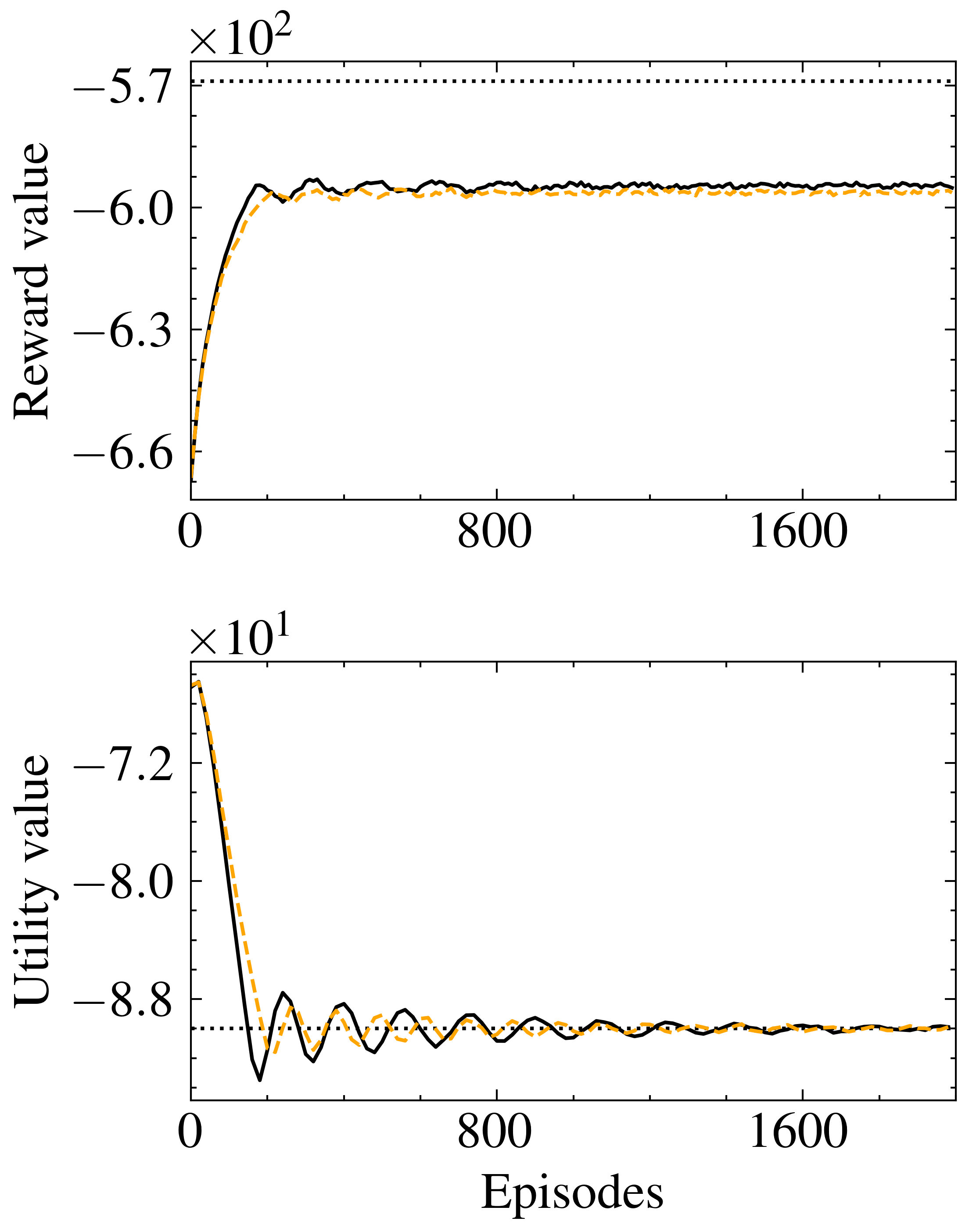
Figure 5: Reward and utility value functions of policy iterates generated by D-PGPD ( ) and AD-PGPD (   ) in the navigation control problem with quadratic rewards.

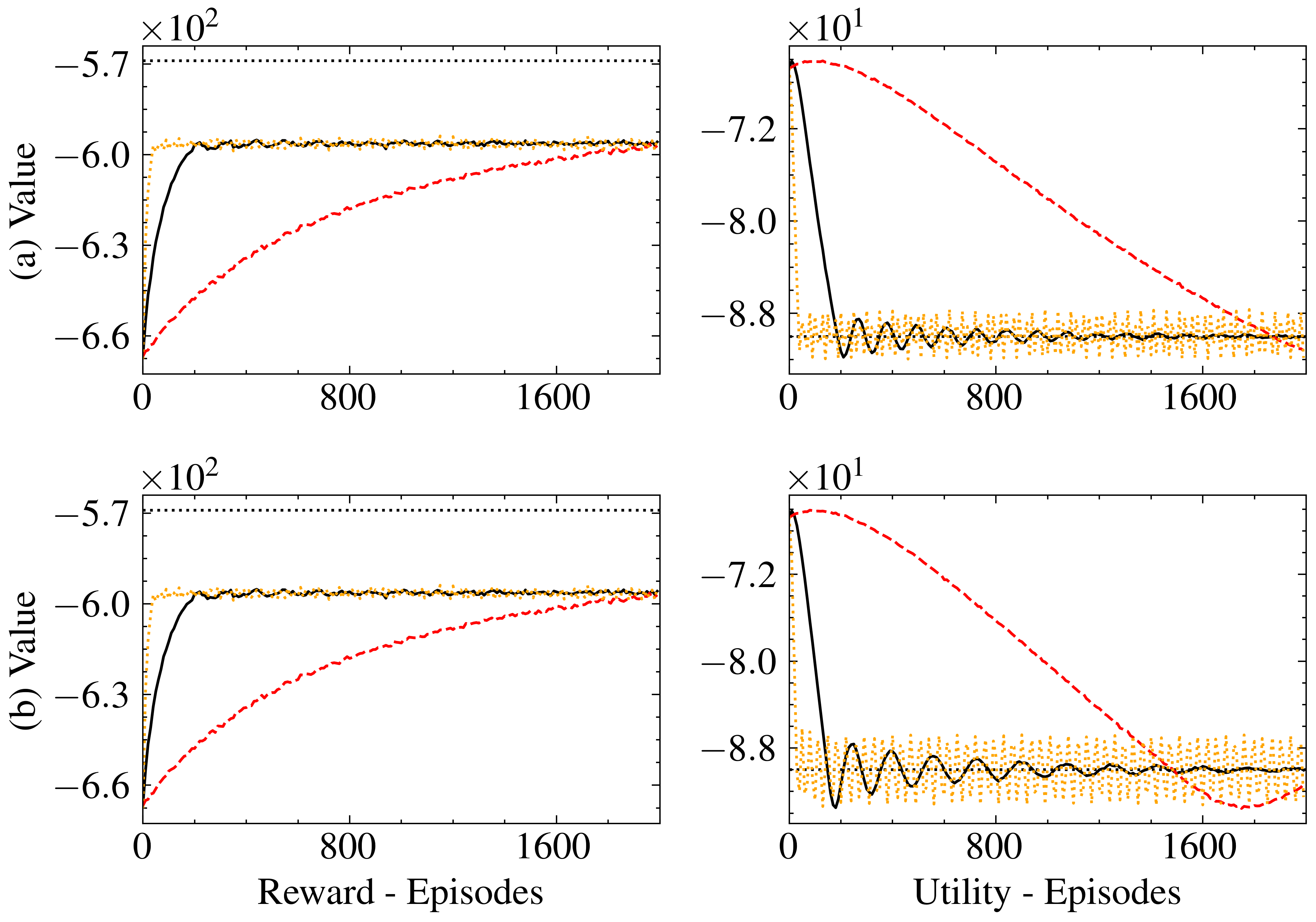
Figure 6: Reward value and utility value for (a) D-PGPD and (b) AD-PGPD in the navigation control problem for different values of the step-size: $\eta=0.1$ (   ), $\eta=0.01$ ( ) and $\eta=0.001$ (   ).

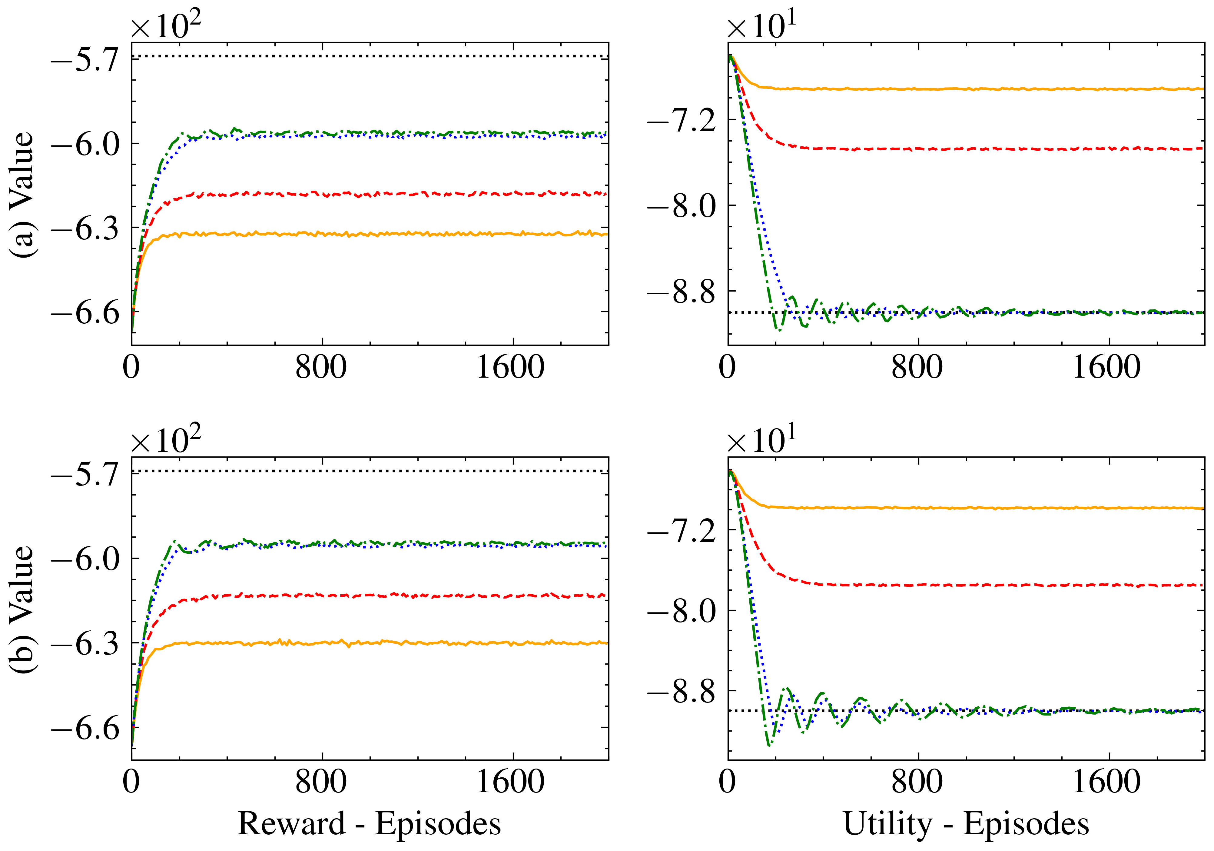
Figure 7: Reward value and utility value for (a) D-PGPD and (b) AD-PGPD in the navigation control problem for different values of the regularization parameter $\tau=1.0$ ( ), $\tau=0.5$ (   ), $\tau=0.1$ (     ), and $\eta=0.01$ (     ).

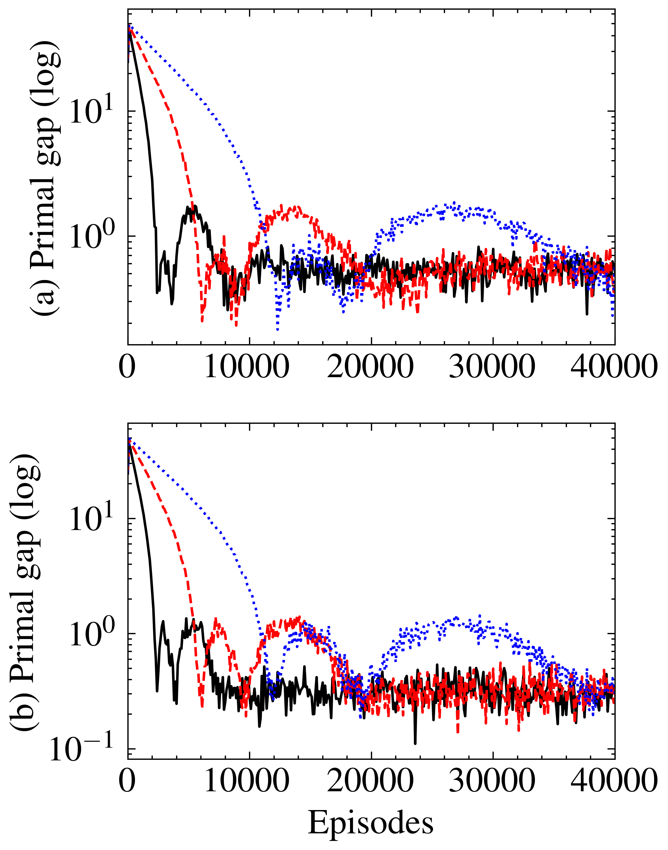
Figure 8: Reward value gap between optimal policy and the iterates of (a) D-PGPD and (b) AD-PGPD $\|V_{r}(\pi_{\tau}^{\star})-V_{r}(\pi_{t})\|$ in the navigation control problem for different values of the step-size: $\eta=0.0005$ ( ), $\eta=0.0002$ (   ) and $\eta=0.0001$ (     ).

Absolute-valued penalty. D-PGPD allows tackling problems that are outside the scope of classical constrained quadratic problems with known dynamics. First of all, we consider the dynamics to be unknown, hence we need to approximate value functions via rollout averages. Therefore, we need to leverage the sample-based formulation of AD-DPPG to address the problem. Second, we consider the reward functions to in absolute value. In fact, absolute-valued penalties are preferred in sample-based scenarios since quadratic penalties can lead to unstable behaviors Engel and Babuška [2014]. We consider the same setup, but now the reward functions are defined as

$$r(s,a)\;=\;\|g_{1}*s\|_{1}+\|m_{1}*a\|_{1}\;\;\text{ and }\;\;u(s,a)\;=\;\|g_{2}*s\|_{1}+\|m_{2}*a\|_{1},$$

where $*$ denotes the Hadamard product, and

$$g_{1}\;=\;\begin{bmatrix}-1&\\ -1&\\ -0.001&\\ -0.001&\end{bmatrix}\;\;\text{ and }\;\;g_{2}\;=\;\begin{bmatrix}-0.001&\\ -0.001&\\ -1&\\ -1&\end{bmatrix},$$

and

$$m_{1}\;=\;\begin{bmatrix}-0.01&\\ -0.01&\end{bmatrix}\;\;\text{ and }\;\;m_{2}\;=\;\begin{bmatrix}-0.01&\\ -0.01&\end{bmatrix}.$$

The default values of the hyper-parameters of this experiment are $\tau=0.2$, $\eta=0.0001$ and b=$-1000$. Again, we have used linear function approximation with the basis function $\phi(s,a)\mathrel{\mathop{:}}=[s^{\top},a^{\top}]^{\top}\otimes[s^{\top},a^{\top}]^{\top}$. We have compared the sample-based AD-PGPD against PGDual, that implements a dual method with a linear model as a function-approximator [Zhao and You, 2021, Brunke et al., 2022]. Fig. 9 shows the average value functions of policy iterates generated by the sample-based version of AD-PGPD and PGDual over $40,000$ iterations, averaged across $50$ experiments. As observed in the previous experiment, the oscillations of AD-PGPD are damped over time, and it converges to a feasible solution. The low variance of the reward and utility value functions indicates that the policies generated by AD-PGPD exhibit near-deterministic behavior and do not violate the constraints. On the other hand, PGDual fails to dampen the oscillations, as evidenced by the large variance in the reward and utility value functions. This implies that PGDual outputs policies that violate the constraints in several episodes. PGDual requires more episodes to reach a solution, but its final performance in terms of primal return is similar to that of AD-PGPD.

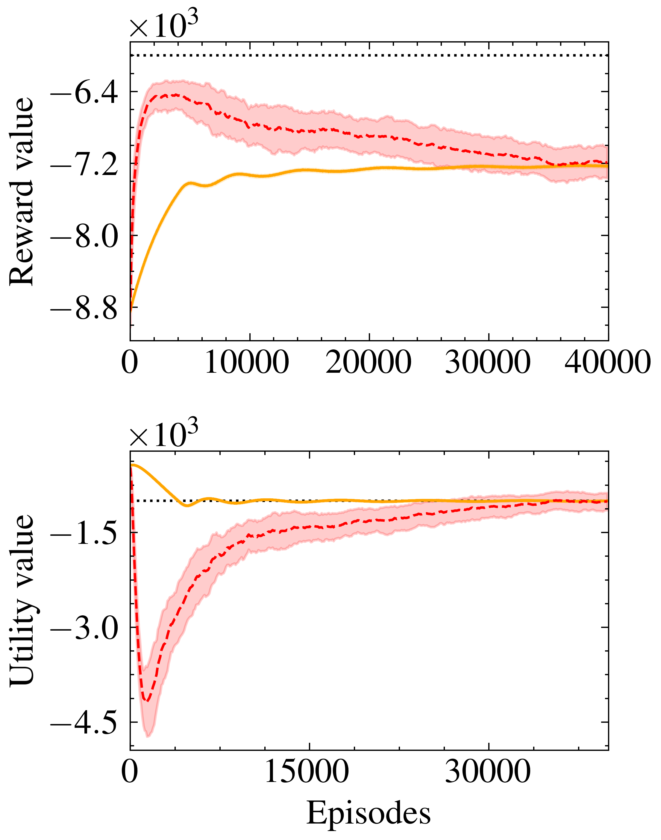
Figure 9: Average reward and utility value functions of policy iterates generated by AD-PGPD ( ) and PGDual (   ) in the navigation control problem with absolute-value rewards.

Zone control. The sample-based AD-PGPD also allows us to deal with non-conventional reward functions. In this third setup, we solve a zone control problem. The agent has to achieve the reference state $s_{r}=[0,0,0,0]$ while minimizing the control action. However, now the constraint imposes that the agent has to remain in the positive orthant. The reward and the utility functions are detailed as follows

$$r(s,a)\;=\;s^{\top}Gs+a^{\top}Ra$$

$$u(s,a)\;=\;\begin{cases}0\;\;&\text{if}\;\;p_{x}\geq 0\;\;\text{and}\;\;p_{y}\geq 0\\ -100\;\;&\text{otherwise},\end{cases}$$

where

$$G\;=\;\begin{bmatrix}-1&\;0&\;0&\;0&\\ 0&\;-1&\;0&\;0&\\ 0&\;0&\;-0.1&\;0&\\ 0&\;0&\;0&\;-0.1&\end{bmatrix}\;\;\text{ and }\;\;R\;=\;\begin{bmatrix}-0.1&\;\;0&\\ 0&\;\;-0.1&\\ \end{bmatrix}.$$

For this experiment the default values are $\tau=0.01$, $\eta=0.00005$ and $b=-200$. We have employed the same basis function $\phi(s,a)\mathrel{\mathop{:}}=[s^{\top},a^{\top}]^{\top}\otimes[s^{\top},a^{\top}]^{\top}$. Again, we have compared the sample-based AD-PGPD against PGDual. Fig. 10 illustrates the value functions of policy iterates generated by the sample-based versions of AD-PGPD and PGDual over $T=50,000$ iterations, averaged across $50$ experiments. The AD-PGPD algorithm effectively dampens oscillations, converging to a feasible solution with low variance in the returns, indicating near-deterministic behavior. Conversely, PGDual not only exhibits a slower convergence rate but also continues to oscillate, frequently violating constraints as evidenced by the high variance associated with its solutions. In terms of reward value, AD-PGPD outperforms PGDual, although the underperformance of the latter is partly attributed to insufficient convergence time.

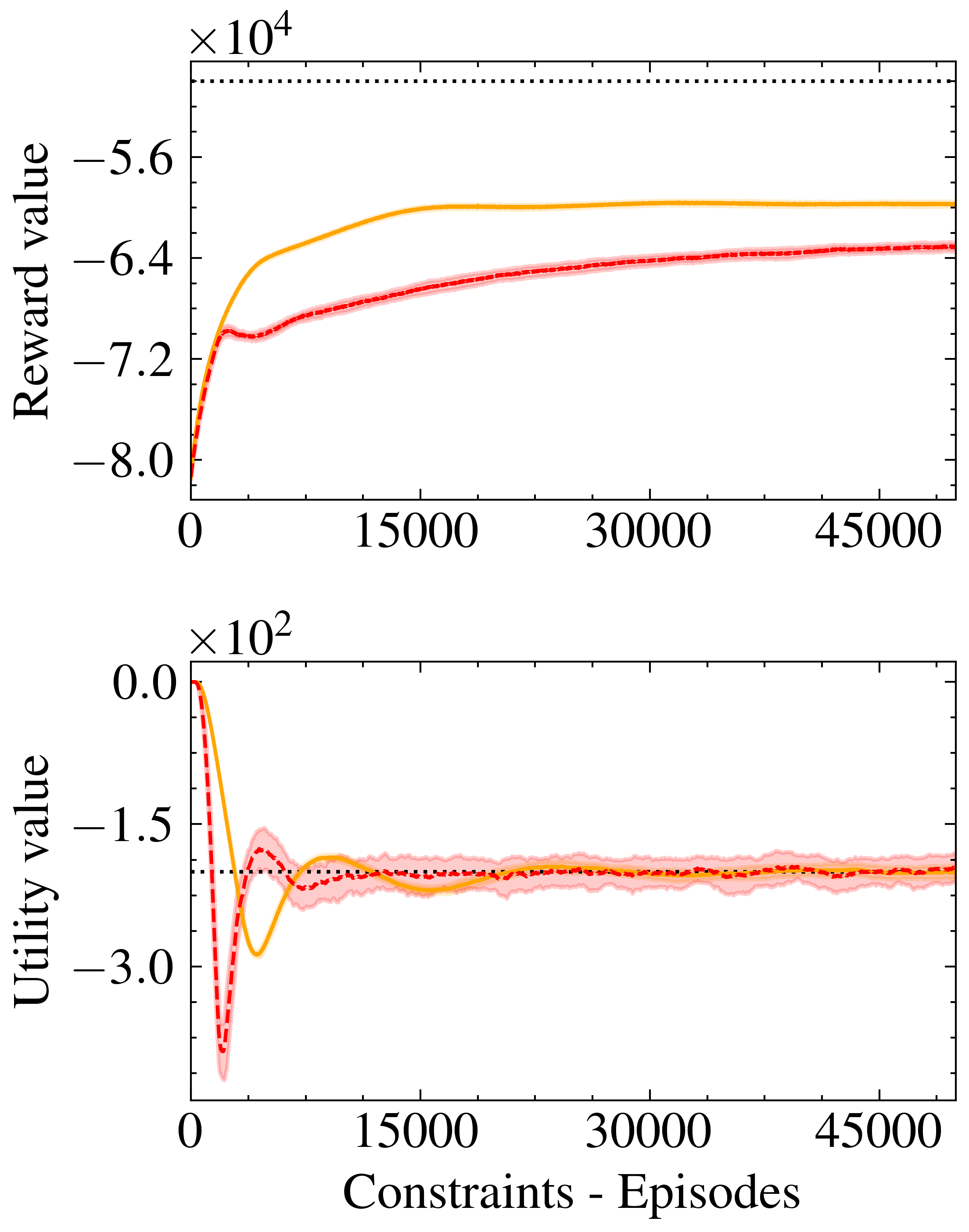
Figure 10: Average reward and utility value functions of policy iterates generated by AD-PGPD ( ) and PGDual (   ) in the navigation control problem with restricted zones.

Figure 11: Average reward and utility value functions of policy iterates generated by AD-PGPD ( ) and PGDual (   ) in a fluid velocity control.

F.2 Non-linear Constrained Regulation

We have assessed the performance of D-PGPD in a non-linear control problem, specifically the control of the velocity of an incompressible Newtonian fluid described by the one-dimensional Burgers’ equation Baker et al. [2000]. The velocity profile $s$ of the fluid varies in a one-dimensional space $x$ bounded in the interval $[0,1]$ and time $t$, described by the equation

$$\frac{\partial s(x,t)}{\partial t} \;=\;\varepsilon\frac{\partial^{2}s(x,t)}{\partial x^{2}}-\frac{1}{2}\frac{\partial(s(x,t)^{2})}{\partial x}+a(t)+\theta_{\text{max}}(t),$$

where $\varepsilon$ is a viscosity coefficient, $\theta_{\text{max}}(t)$ is some Brownian noise, and $a$ is the bounded control action, such as the injection of polymers or mass transport through porous walls. The initial condition is given by $s(\cdot,0)\sim\rho$, where $\rho$ is the initial state distribution.

We discretize the dynamics of the system using an Euler scheme Borggaard and Zietsman [2020]. This approach converts the continuous partial differential equation into a discrete form suitable for numerical computation. The spatial domain $[0,1]$ is divided into $d$ intervals, resulting in a grid with points $x_{i}=\frac{i}{d}$ for $i=0,1,\ldots,d$. The velocity profile $s(x,t)$ is approximated at these grid points, resulting in a vector $s_{t}$ at each time-step $t$. Time is discretized into steps of size $\Delta t$, with $t=k\Delta t$ for $k=0,1,2,\ldots$ The time derivative is approximated using a forward Euler method,

$$\frac{\partial s(x,t)}{\partial t}\;\approx\;\frac{s(x,t+\Delta t)-s(x,t)}{\Delta t}.$$

The spatial derivatives $\partial^{2}s/\partial x^{2}$ and $\partial(s^{2})\partial x$ are approximated using finite differences. The discretized form of Burgers’ equation at each grid point $x_{i}$ and time-step $t$ is given by

$$\frac{s_{i}^{t+1}-s_{i}^{t}}{\Delta t} \;=\;\varepsilon\frac{s_{i+1}^{t}-2s_{i}^{t}+s_{i-1}^{t}}{(\Delta x)^{2}}-\frac{1}{2}\left(\frac{(s_{i+1}^{t})^{2}-(s_{i-1}^{t})^{2}}{2\Delta x}\right)+a^{t}_{i}+\omega_{i}^{t},$$

where $\omega_{i}^{t}$ is Gaussian noise, and $a_{i}^{t}$ is the control action at point $x_{i}$. Rearranging gives

$$s_{i}^{t+1} \;=\;s_{i}^{t}+\Delta t\left(\varepsilon\frac{s_{i+1}^{t}-2s_{i}^{t}+s_{i-1}^{t}}{(\Delta x)^{2}}-\frac{1}{2}\left(\frac{(s_{i+1}^{t})^{2}-(s_{i-1}^{t})^{2}}{2\Delta x}\right)+a_{i}^{t}+\omega_{t}\right).$$

The discretized dynamics of the system can then be expressed in matrix form as the non-linear system

$$s_{t+1}\;=\;B_{0}s_{t}+B_{1}a_{t}+B_{2}s_{t}^{2}+\omega_{t},$$

where $s_{t}^{2}$ is the element-wise squared state, the dimensionality of the state-action space is $d=d_{s}=d_{a}$, and $B_{0}$, $B_{1}$, $B_{2}\in{\mathbb{R}}^{d\times d}$ are matrices representing the discretized spatial operators and non-linear terms, and $a_{t}\in{\mathbb{R}}^{n}$ is the control input vector. In the proposed scenario, we have selected a discrete grid of $d=10$, a time-step $\Delta t=0.01$, and a viscosity coefficient $\varepsilon=0.1$.

The goal is to drive the velocity of the fluid towards $0$, while minimizing the control action. Furthermore, we introduce a constraint to limit the expected control action that the agent can employ. To that end, consider the reward and utility functions

$$r(s,a) \;=\;-\|s\|^{2}\;\;\text{ and }\;\;u(s,a)\;=\;-\|a\|_{1}.$$

The parameters of this experiment are $\tau=0.001$, $\eta=0.001$, and $b=-20$. We have compared the sample-based AD-PGPD against PGDual. The basis function of the function approximation is $\phi(s,a)=[s^{\top},a^{\top}]^{\top}\otimes[s^{\top},a^{\top}]^{\top}$. The value functions of policy iterates generated by the sample-based version of AD-PGPD and PGDual over $10,000$ iterations averaged across $50$ experiments can be seen in Fig. 11. The results are consistent with what we have observed in the navigation problem. The AD-PGPD algorithm successfully mitigates oscillations and converges to a feasible solution with low return variance. In contrast, although PGDual achieves similar objective value, it does not dampens oscillations, as indicated by the high variance in its solutions.

References

- Achiam et al. (2017) Joshua Achiam, David Held, Aviv Tamar, and Pieter Abbeel. Constrained policy optimization. In International Conference on Machine Learning, pages 22–31, 2017.
- Agarwal et al. (2021) Alekh Agarwal, Sham M Kakade, Jason D Lee, and Gaurav Mahajan. On the theory of policy gradient methods: Optimality, approximation, and distribution shift. Journal of Machine Learning Research, 22(98):1–76, 2021.
- Altman (2021) Eitan Altman. Constrained Markov Decision Processes. Routledge, 2021.
- Anderson and Moore (2007) Brian DO Anderson and John B Moore. Optimal Control: Linear Quadratic Methods. Courier Corporation, 2007.
- Auslender and Teboulle (2006) Alfred Auslender and Marc Teboulle. Asymptotic Cones and Functions in Optimization and Variational Inequalities. Springer Science & Business Media, 2006.
- Baker et al. (2000) James Baker, Antonios Armaou, and Panagiotis D Christofides. Nonlinear control of incompressible fluid flow: Application to burgers’ equation and 2d channel flow. Journal of Mathematical Analysis and Applications, 252(1):230–255, 2000.
- Bemporad et al. (2002) Alberto Bemporad, Manfred Morari, Vivek Dua, and Efstratios N Pistikopoulos. The explicit linear quadratic regulator for constrained systems. Automatica, 38(1):3–20, 2002.
- Borggaard and Zietsman (2020) Jeff Borggaard and Lizette Zietsman. The quadratic-quadratic regulator problem: Approximating feedback controls for quadratic-in-state nonlinear systems. In American Control Conference, pages 818–823, 2020.
- Brunke et al. (2022) Lukas Brunke, Melissa Greeff, Adam W Hall, Zhaocong Yuan, Siqi Zhou, Jacopo Panerati, and Angela P Schoellig. Safe learning in robotics: From learning-based control to safe reinforcement learning. Annual Review of Control, Robotics, and Autonomous Systems, 5:411–444, 2022.
- Calvo-Fullana et al. (2023) Miguel Calvo-Fullana, Santiago Paternain, Luiz FO Chamon, and Alejandro Ribeiro. State augmented constrained reinforcement learning: Overcoming the limitations of learning with rewards. IEEE Transactions on Automatic Control, 2023.
- Chow et al. (2018) Yinlam Chow, Mohammad Ghavamzadeh, Lucas Janson, and Marco Pavone. Risk-constrained reinforcement learning with percentile risk criteria. Journal of Machine Learning Research, 18(167):1–51, 2018.
- Cruz-Suárez et al. (2004) Daniel Cruz-Suárez, Raúl Montes-de Oca, and Francisco Salem-Silva. Conditions for the uniqueness of optimal policies of discounted markov decision processes. Mathematical Methods of Operations Research, 60:415–436, 2004.
- Ding et al. (2022) Dongsheng Ding, Kaiqing Zhang, Jiali Duan, Tamer Başar, and Mihailo R Jovanović. Convergence and sample complexity of natural policy gradient primal-dual methods for constrained mdps. arXiv preprint arXiv:2206.02346, 2022.
- Ding et al. (2024a) Dongsheng Ding, Zhengyan Huan, and Alejandro Ribeiro. Resilient constrained reinforcement learning. In International Conference on Artificial Intelligence and Statistics, pages 3412–3420, 2024a.
- Ding et al. (2024b) Dongsheng Ding, Chen-Yu Wei, Kaiqing Zhang, and Alejandro Ribeiro. Last-iterate convergent policy gradient primal-dual methods for constrained mdps. Advances in Neural Information Processing Systems, 36, 2024b.
- Dolgov (2005) Dmitri Dolgov. Stationary deterministic policies for constrained mdps with multiple rewards, costs, and discount factors. In International Joint Conference on Artificial Intelligence, 2005.
- Engel and Babuška (2014) Jan-Maarten Engel and Robert Babuška. On-line reinforcement learning for nonlinear motion control: Quadratic and non-quadratic reward functions. IFAC Proceedings Volumes, 47(3):7043–7048, 2014.
- Feinberg (2000) Eugene A Feinberg. Constrained discounted markov decision processes and hamiltonian cycles. Mathematics of Operations Research, 25(1):130–140, 2000.
- Feinberg and Piunovskiy (2002) Eugene A Feinberg and Aleksey B Piunovskiy. Nonatomic total rewards markov decision processes with multiple criteria. Journal of Mathematical Analysis and Applications, 273(1):93–111, 2002.
- Feinberg and Piunovskiy (2019) Eugene A Feinberg and Alexey Piunovskiy. Sufficiency of deterministic policies for atomless discounted and uniformly absorbing mdps with multiple criteria. SIAM Journal on Control and Optimization, 57(1):163–191, 2019.
- Gao et al. (2023) Xiaoshan Gao, Liang Yan, Zhijun Li, Gang Wang, and I-Ming Chen. Improved deep deterministic policy gradient for dynamic obstacle avoidance of mobile robot. IEEE Transactions on Systems, Man, and Cybernetics: Systems, 53(6):3675–3682, 2023.
- Garg et al. (2020) Kunal Garg, Ehsan Arabi, and Dimitra Panagou. Prescribed-time convergence with input constraints: A control lyapunov function based approach. In American Control Conference, pages 962–967, 2020.
- Kakade et al. (2020) Sham Kakade, Akshay Krishnamurthy, Kendall Lowrey, Motoya Ohnishi, and Wen Sun. Information theoretic regret bounds for online nonlinear control. Advances in Neural Information Processing Systems, 33:15312–15325, 2020.
- Kumar et al. (2020) Harshat Kumar, Dionysios S Kalogerias, George J Pappas, and Alejandro Ribeiro. Zeroth-order deterministic policy gradient. arXiv preprint arXiv:2006.07314, 2020.
- Lacoste-Julien et al. (2012) Simon Lacoste-Julien, Mark Schmidt, and Francis Bach. A simpler approach to obtaining an o (1/t) convergence rate for the projected stochastic subgradient method. HAL, 2012, 2012.
- Lan (2020) Guanghui Lan. First-Order and Stochastic Optimization Methods for Machine Learning, volume 1. Springer, 2020.
- Lan (2022) Guanghui Lan. Policy optimization over general state and action spaces. arXiv preprint arXiv:2211.16715, 2022.
- Li et al. (2022) Guofa Li, Shenglong Li, Shen Li, and Xingda Qu. Continuous decision-making for autonomous driving at intersections using deep deterministic policy gradient. IET Intelligent Transport Systems, 16(12):1669–1681, 2022.
- Li et al. (2023) Zihao Li, Boyi Liu, Zhuoran Yang, Zhaoran Wang, and Mengdi Wang. Double duality: Variational primal-dual policy optimization for constrained reinforcement learning. Journal of Machine Learning Research, 24(385):1–43, 2023.
- Lillicrap et al. (2015) Timothy P Lillicrap, Jonathan J Hunt, Alexander Pritzel, Nicolas Heess, Tom Erez, Yuval Tassa, David Silver, and Daan Wierstra. Continuous control with deep reinforcement learning. arXiv preprint arXiv:1509.02971, 2015.
- Lim and Zhou (1999) Andrew EB Lim and Xun Yu Zhou. Stochastic optimal lqr control with integral quadratic constraints and indefinite control weights. IEEE Transactions on Automatic Control, 44(7):1359–1369, 1999.
- Ma et al. (2022) Jun Ma, Zilong Cheng, Xiaoxue Zhang, Masayoshi Tomizuka, and Tong Heng Lee. Alternating direction method of multipliers for constrained iterative lqr in autonomous driving. IEEE Transactions on Intelligent Transportation Systems, 23(12):23031–23042, 2022.
- Mandhane et al. (2022) Amol Mandhane, Anton Zhernov, Maribeth Rauh, Chenjie Gu, Miaosen Wang, Flora Xue, Wendy Shang, Derek Pang, Rene Claus, Ching-Han Chiang, et al. Muzero with self-competition for rate control in vp9 video compression. arXiv preprint arXiv:2202.06626, 2022.
- McMahan (2024) Jeremy McMahan. Deterministic policies for constrained reinforcement learning in polynomial-time. arXiv preprint arXiv:2405.14183, 2024.
- Montes-de Oca et al. (2013) Raúl Montes-de Oca, Enrique Lemus-Rodríguez, and Francisco Sergio Salem-Silva. Nonuniqueness versus uniqueness of optimal policies in convex discounted markov decision processes. Journal of Applied Mathematics, 2013, 2013.
- Moskovitz et al. (2023) Ted Moskovitz, Brendan O’Donoghue, Vivek Veeriah, Sebastian Flennerhag, Satinder Singh, and Tom Zahavy. Reload: Reinforcement learning with optimistic ascent-descent for last-iterate convergence in constrained mdps. In International Conference on Machine Learning, pages 25303–25336, 2023.
- Paternain et al. (2019) Santiago Paternain, Luiz Chamon, Miguel Calvo-Fullana, and Alejandro Ribeiro. Constrained reinforcement learning has zero duality gap. Advances in Neural Information Processing Systems, 32, 2019.
- Paternain et al. (2020) Santiago Paternain, Juan Andrés Bazerque, Austin Small, and Alejandro Ribeiro. Stochastic policy gradient ascent in reproducing kernel hilbert spaces. IEEE Transactions on Automatic Control, 66(8):3429–3444, 2020.
- Paternain et al. (2022) Santiago Paternain, Miguel Calvo-Fullana, Luiz FO Chamon, and Alejandro Ribeiro. Safe policies for reinforcement learning via primal-dual methods. IEEE Transactions on Automatic Control, 68(3):1321–1336, 2022.
- Posa et al. (2016) Michael Posa, Scott Kuindersma, and Russ Tedrake. Optimization and stabilization of trajectories for constrained dynamical systems. In IEEE International Conference on Robotics and Automation, pages 1366–1373, 2016.
- Ross (1989) Keith W Ross. Randomized and past-dependent policies for markov decision processes with multiple constraints. Operations Research, 37(3):474–477, 1989.
- Ruszczyński (2006) Andrzej P Ruszczyński. Nonlinear Optimization, volume 13. Princeton University Press, 2006.
- Scokaert and Rawlings (1998) Pierre OM Scokaert and James B Rawlings. Constrained linear quadratic regulation. IEEE Transactions on Automatic Control, 43(8):1163–1169, 1998.
- Shimizu et al. (2020) Yutaka Shimizu, Wei Zhan, Liting Sun, Jianyu Chen, Shinpei Kato, and Masayoshi Tomizuka. Motion planning for autonomous driving with extended constrained iterative lqr. In Dynamic Systems and Control Conference, volume 84270, page V001T12A001, 2020.
- Silver et al. (2014) David Silver, Guy Lever, Nicolas Heess, Thomas Degris, Daan Wierstra, and Martin Riedmiller. Deterministic policy gradient algorithms. In International Conference on Machine Learning, pages 387–395, 2014.
- Stathopoulos et al. (2016) Giorgos Stathopoulos, Milan Korda, and Colin N Jones. Solving the infinite-horizon constrained lqr problem using accelerated dual proximal methods. IEEE Transactions on Automatic Control, 62(4):1752–1767, 2016.
- Tessler et al. (2018) Chen Tessler, Daniel J Mankowitz, and Shie Mannor. Reward constrained policy optimization. arXiv preprint arXiv:1805.11074, 2018.
- Tsiamis et al. (2020) Anastasios Tsiamis, Dionysios S Kalogerias, Luiz FO Chamon, Alejandro Ribeiro, and George J Pappas. Risk-constrained linear-quadratic regulators. In IEEE Conference on Decision and Control, pages 3040–3047. IEEE, 2020.
- Tsiamis et al. (2021) Anastasios Tsiamis, Dionysios S Kalogerias, Alejandro Ribeiro, and George J Pappas. Linear quadratic control with risk constraints. arXiv preprint arXiv:2112.07564, 2021.
- Zahavy et al. (2021) Tom Zahavy, Brendan O’Donoghue, Guillaume Desjardins, and Satinder Singh. Reward is enough for convex mdps. Advances in Neural Information Processing Systems, 34:25746–25759, 2021.
- Zhang et al. (2020) Kaiqing Zhang, Alec Koppel, Hao Zhu, and Tamer Basar. Global convergence of policy gradient methods to (almost) locally optimal policies. SIAM Journal on Control and Optimization, 58(6):3586–3612, 2020.
- Zhao and You (2021) Feiran Zhao and Keyou You. Primal-dual learning for the model-free risk-constrained linear quadratic regulator. In Learning for Dynamics and Control, pages 702–714, 2021.
- Zhao et al. (2021) Feiran Zhao, Keyou You, and Tamer Başar. Infinite-horizon risk-constrained linear quadratic regulator with average cost. In IEEE Conference on Decision and Control, pages 390–395, 2021.
- Zinkevich (2003) Martin Zinkevich. Online convex programming and generalized infinitesimal gradient ascent. In International Conference on Machine Learning, pages 928–936, 2003.