Sustainability of distribution of entanglement in tripartite systems under dephasing environment

Abstract

Preserving multipartite entanglement amidst decoherence poses a pivotal challenge in quantum information processing. Also the measurement of multipartite entanglement in mixed states amid decoherence presents a formidable task. Employing reservoir memory offers a means to attenuate the decoherence dynamics impacting multipartite entanglement, slowing its degradation. In this work, we investigate the distribution of entanglement in tripartite systems for both pure and mixed states under a structured dephasing environment at finite temperature under both Markovian and Non-Markovian dynamics. Here, we consider situation where the three qubits in a common reservoir and also the situation where each qubit is in a local bosonic reservoir. We have also shown that the robustness of a quantum system to decoherence depends on the distribution of entanglement and its interaction with the different configurations of the bath. When each qubit has its own local environment, the system exhibits different dynamics compared to when all three qubits share a common environment. Furthermore, in the presence of the reservoir memory, the sustainability of distribution of entanglement in a tripartite system under dephasing dynamics is significantly enhanced.

I Introduction

Entanglement is an incredible feature of quantum many-body systems and its investigation has both theoretical and practical significance [1]. Beyond its foundational importance, entanglement dynamics and its distribution also play an important role in quantum information processing tasks such as quantum teleportation [2], quantum dense coding [3], quantum cryptography [4], quantum computing [5] and many more. The real world success of quantum information processing therefore, relies on the longevity of entanglement in quantum states. However, quantum systems interact to surrounding environment causing decoherence, resulting to the loss of quantum features like entanglement and coherence [6, 7]. It is therefore important to study the distribution of entanglement in multipartite scenario. Various methods have been developed to circumvent this detrimental effect of decoherence, viz. quantum error correction [8, 9], finding decoherence-free subspace [10, 11], and dynamical decoupling [12, 13]. There is another approach which is relatively new, known as environment engineering or reservoir engineering [14, 15, 16, 17, 18]. We adopt here this approach of engineering where the coupling between system and environment is modified to enhance the longevity of multipartite entanglement. In this approach, one can structure the reservoir spectrum in such a way that the reservoir memory effects are significant to slow down the decay process. Our aim is to identify various pure and mixed tripartite entangled states whose distribution of entanglement among various parties are robust against decoherence effects.

Under the influence of the environment, quantum dynamics of the system is described by a non-unitary time evolution of the reduced density matrix, and the resulting open system dynamics can be Markovian or Non-Markovian [19, 20]. It was shown that Non-Markovian dynamics of two-qubit entangled states can be strikingly different from their Markovian counterparts [17, 21, 22, 23, 24, 25, 26]. Extensive study of the dynamics of entanglement in multipartite open quantum systems under the consequences of environmental effects has become a matter of active research in recent years [18, 27, 28, 29, 30, 31, 32]. One of the barriers in such type of study is the non-existence of a good measure of entanglement of multipartite quantum states. A good entanglement measure should be able to accurately reflect the operational time scale of the quantum device with respect to a quantum information processing task. In this regard, we are going to investigate multipartite entanglement distribution dynamics in the presence of a structured dephasing environment at finite temperature [33, 34, 35]. We have considered both the situations when individual qubits interact with its local environment or all the qubits collectively interact with a common environment. In this respect, the sustainability of distribution of entanglement of various pure and mixed multipartite entangled states are examined under (a) local Markov (b) local Non-Markov (c) common Markov and (d) common Non-Markov dephasing environment. The paper is organized as follows. In Sec. 2 we give a brief review of the various entanglement measures and the measure we use in our study. An overview of the open system model is discussed in Sec. 3. The fourth section describes the dynamics of entanglement in pure and mixed states for both Markovian and Non-Markovian environment. Finally we present our conclusions in the section 5.

II Multipartite Entanglement Measure and distribution of entanglement

Entanglement in bipartite systems is quantified using concurrence [36]. In general entanglment decoheres under the action of environment and these effects can be quantified for bipartite systems using concurrence. When we start investigating entanglement in multipartite systems and the effect of environment on the entanglement, we need use more general multipartite measures of entanglement. Some of the well known measures of multipartite entanglement are generalized concurrence [37], tangle [38], $n$-tangle [39] , negativity [40, 41]. To compute the generalized concurrence we need to do a convex optimization. The tangle of a tripartite system is a potential way to quantify the amount of tripartite entanglement in the system, but its generalization namely the $n$-tangle is not invariant under permutations of qubits for general odd $n$ over $3$ and hence is not a useful measure [39]. Negativity on the other hand, used mostly in bipartite system but rarely in studying multipartite entanglement as for two qubit system the negativity as measure of entanglement is both necessary and sufficient condition, while for multipartite system, this is not the case. We in this article, have used relative entropy of entanglement as the measure to study the entanglement dynamics of the 3-qubit systems under considerations.

An alternative approach to measure entanglement is to use the relative entropy of entanglement. In this method we quantify how much an entangled state can be operationally distinguished from the set of separable states [42, 43]. This measure is intimately connected to the entanglement of distillation by providing an upper bound for it. If $\mathcal{D}$ is the set of all disentangled states, the measure of entanglement for a state $\rho$ is defined as

$$E(\rho)=\min_{\sigma\in\mathcal{D}}S(\rho||\sigma),$$ (1)

where $\rho$ is the given density matrix and $\sigma$ is a separable state. The entanglement is found by measuring the distance of $\rho$ to the closest separable state. Here $S(\rho||\sigma)$ is the quantum relative entropy, defined as

$$S(\rho||\sigma)={\rm Tr}\{\rho(\ln\rho-\ln\sigma)\},$$ (2)

and this measure works for quantum states of arbitrary dimensions. The state $\rho$ on the boundary of separable states is called the closest separable state. The measure (1) gives the amount of entanglement in the density matrix from the set of disentangled states. From the statistical point of view, it is known that the more entangled a state is, the more it is distinguishable from a disentangled state.

In bipartite systems, the entire entanglement is present between the two parties. When we have multipartite systems, the entanglement can be distributed in different ways. For example if we consider tripartite systems, the entanglement can be distributed between all the three qubits in a genuinely multipartite fashion or in a relatively local manner. In a genuninely multipartite entanglement, the loss of a single qubit to external decoherence leads to the loss of entire entanglement in the system. An example of such a state is the GHZ state where the loss of single qubit leads to a completed decohered bipartite system. There are some multipartite systems in which the decoherence of a qubit does not automatically lead to the loss of entire entanglement in the system. The $W$ states is a perfect example of such systems. In these states the three qubits are entangled in mutually pairwise fashion and so if one qubit decoheres, the entanglement between the other pair is still preserved. The entanglement distribution is a very important concept to understand the robustness of entanglement in multipartite systems. To investigate this we use the idea of the following inequality, which is defined as

$$E_{A:BC}\geq E_{A:B}+E_{B:C}$$ (3)

where $E_{A:BC}$ is the entanglement between the qubit $A$ and the bipartite block $BC$, similarly $E_{A:B}$ is the entanglement between the qubits $A$ and $B$ after tracing out qubit $C$. If this inequality holds we can observe that the genuine tripartite entanglement is higher, if not the bipartite entanglements are higher. To analyse the entanglement distribution we recast the relation (3) as

$$D=|E_{A:BC}-E_{A:B}-E_{A:C}|,$$ (4)

This expression is used to investigate the distribution of entanglement in tripartite systems. We are investing only the modulus value since we wish to compare the decrease of the distribution of entanglement, and we do not want to keep track of whether the entanglement is genuine multipartite entanglement or bipartite entanglement. In our work we are studying open quantum systems which are subjected to dephasing environment, so the entanglement distribution will also be dynamically varying and so the quantity $D$ will also be a function of time.

III Description of the Models

To study the entanglement dynamics in an open quantum system, we investigate a three qubit system in contact with an external bath which simulates the environment. Due to the interaction with the external environment, entanglement decreases with time. In this work we examine the change in the distribution of entanglement due to the external dephasing environment. We consider two different situations where the three qubits are in (i) local dephasing environment, i.e., each qubit in its own dephasing environment and (ii) common dephasing environment where all the qubits are exposed to one single dephasing environment.

III.1 Three Qubits Under Local Dephasing Environment

A spin-boson model of three non-interacting qubits each of which is interacting with a local bosonic reservoir is considered. A schematic picture of this model is shown in Fig. $1(a)$. The total Hamiltonian of the three qubits along with its environment is

$$H=\sum_{i=1}^{3}\Big{[}\frac{\hslash}{2}\omega_{0}^{i}\sigma_{z}^{i}+\sum_{k}\hslash\omega_{ik}b_{ik}^{\dagger}b_{ik}+\sigma_{z}^{i}(B_{i}+B_{i}^{\dagger})\Big{]}.$$ (5)

Here $\omega_{0}^{i}$ and $\sigma_{z}^{i}$ correspond to the transition frequency and the Pauli spin operator respectively. In our work we assume that all these qubits have the same transition frequency $\omega_{0}^{i}=\omega_{0}$. Also $B_{i}=\sum_{k}g_{ik}b_{ik}$, where $b_{ik}^{\dagger}$ ($b_{ik}$) is the creation (annihilation) operator associated with the $k^{th}$ mode of the local environment interacting with the $i^{th}$ qubit. The factor $g_{ik}$ represents the coupling strength between the $i^{th}$ qubit and its local environment. In the continuum limit, $\sum_{k}|g_{ik}|^{2}\rightarrow\int d\omega J_{i}(\omega)\delta(\omega_{ik}-\omega)$, where $J_{i}(\omega)$ is the spectral density associated to the local environment of the $i^{th}$ qubit.

Initially the three-qubit system is decoupled from the environment, with each environment in a thermal bath $T_{i}$. The Hamiltonian of the composite sytem consisting of the qubits and the environment evolves with time. To study the entanglement dynamics of the qubit system, we need to trace out the environment degrees of the freedom. This gives us the reduced density matrix $\rho(t)$ of the three qubit system from which we can infer the transient dynamics of entanglement. The decay dynamics of the reduced density matrix $\rho(t)$ of the three qubit system under local dephasing can be described by the quantum master equation:

$$\frac{d}{dt}\rho(t)=\sum_{i=1}^{3}\gamma_{i}(t)\Big{(}\sigma_{z}^{i}\rho(t)\sigma_{z}^{i}-\rho(t)\Big{)},$$ (6)

where

$$\gamma_{i}(t)=2\int_{0}^{\infty}d\omega J_{i}(\omega)\coth\left(\frac{\hbar\omega}{2k_{B}T_{i}}\right)\frac{\sin(\omega t)}{\omega}.$$ (7)

The time dependent dephasing rate $\gamma_{i}(t)$ is determined by the spectral density $J_{i}(\omega)$ and for our study we consider the Ohmic-type spectral density [45] which reads as:

$$J_{i}(\omega)=\eta_{i}\omega\exp\left(-\frac{\omega}{\Lambda_{i}}\right).$$ (8)

In general the environment is large enough to quickly reset the state back to its initial value. But in our work we examine the situation where the reservoir memory has an effect on the entanglement dynamics of the $3$-qubit states resulting in a finite cut-off frequency $\Lambda_{i}$. Under the Markov approximation, the correlation time of the environment is much smaller than the time scale of the system dynamics. Hence one can replace the time-dependent coefficient $\gamma_{i}(t)$ by its long-time Markov value $\gamma_{i}^{M}=4\pi\eta_{i}k_{B}T_{i}/\hbar$. In this situation, the decay dynamics of the density matrix $\rho(t)$ is defined as Markovian. The decay constant $\gamma_{i}^{M}$ becomes equal to a fixed value $\gamma_{0}=4\pi\eta k_{B}T/\hbar$ if we assume uniform spectral densities with uniform coupling strengths $\eta_{i}=\eta$, and temperatures $T_{i}=T$ for individual local environments.

III.2 Three Qubits Under Common Dephasing Environment

Next, we consider the situation where the three qubits are in contact with a common reservoir. The microscopic Hamiltonian of the three two-level systems coupled to the common environment is given by

$$H=\frac{\hbar}{2}\sum_{i=1}^{3}\Big{[}\omega_{0}^{i}\sigma_{z}^{i}+\sum_{k}\hbar\omega_{k}b_{k}^{\dagger}b_{k}+S_{z}\left(B+B^{\dagger}\right)\Big{]}.$$ (9)

Here $S_{z}=\sum_{i}\sigma_{z}^{i}$ is the collective spin operator for the three-qubit system. For the common bath the reservoir operator is $B=\hbar\sum_{k}g_{k}b_{k}$ where $b_{k}$ and $b_{k}^{\dagger}$ are annihilation and creation operators associated to $k$th mode of the environment.The common environment is modelled as a collection of bosonic field modes with frequencies $\omega_{k}$. We assume that all three qubits have same transition frequency $\omega_{0}^{i}=\omega_{0}$. We consider a initial state in which the system-environment is factorized and the environment is initially at thermal equilibrium. The quantum master equation when all the three qubits interact with a common dephasing environment at finite temperature is

$$\frac{d}{dt}\rho(t)\!=\!\gamma_{0}tS_{z}\rho(t)S_{z}\!-\!\alpha(t)S_{z}S_{z}\rho(t)\!-\!\alpha^{\ast}(t)\rho(t)S_{z}S_{z},$$

(10)

where

$$\alpha(t) = \int_{0}^{\infty}d\omega J(\omega)\coth\left(\frac{\hbar\omega}{2k_{B}T}\right)\frac{\sin(\omega t)}{\omega}$$ (11)

$$- i\int_{0}^{\infty}d\omega J(\omega)\frac{1-\cos(\omega t)}{\omega}.$$

Under the Markov approximation i.e., when the reservoir memory is negligible, the quantum master equation is of the form:

$$\frac{d}{dt}\rho(t)=\frac{\gamma_{0}}{2}\Big{(}2S_{z}\rho(t)S_{z}-S_{z}S_{z}\rho(t)-\rho(t)S_{z}S_{z}\Big{)}.$$ (12)

Next, by taking specific three qubit states, we show how reservoir memory effects can improve the robustness of the multiqubit entanglement under common environment. The entanglement dynamics is discussed for both Markov and Non-Markov dephasing for an Ohmic spectral density $J(\omega)=\eta\omega\exp(-\omega/\Lambda)$. In our numerical calculation, we choose $k_{B}T=\hbar\omega_{0}/4\pi$ for which $\gamma_{0}=\eta\omega_{0}$ and take $\eta=0.1$, and $\Lambda=10^{-2}\omega_{0}$.

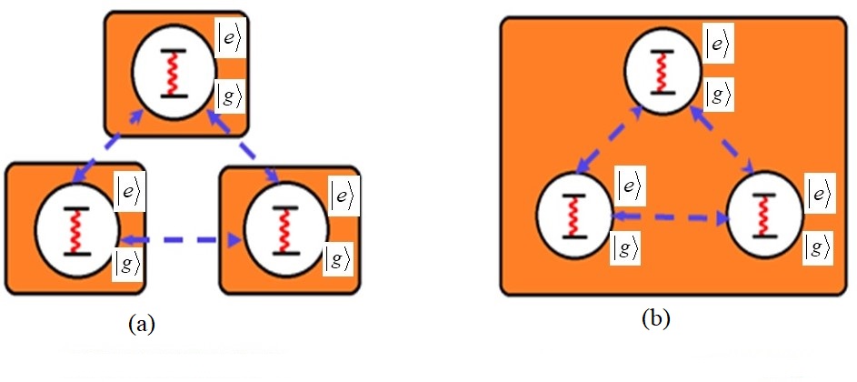
Figure 1: A schematic figure of tripartite state in (a) local environment and in (b) common environment. The three qubits in the system are entangled states. Here $|g\rangle$ denotes ground state and $|e\rangle$ stands for excited state.

IV Results and Discussion

IV.1 Pure states under dephasing environment

The distribution of entanglement of tripartite pure states is studied in a dephasing environment. For our investigations we have considered tripartite pure states such as $|GHZ\rangle$, $|W\rangle$, $|W\bar{W}\rangle$ and $|Star\rangle$ [46, 47, 48]. The GHZ and the W states studied in our work are:

$$|GHZ\rangle=\frac{1}{\sqrt{2}}\Big{(}|000\rangle+|111\rangle\Big{)};\qquad\quad|W\rangle=\frac{1}{\sqrt{3}}\Big{(}|001\rangle+|010\rangle+|100\rangle\Big{)}.$$ (13)

Based on Stochastic Local Operations and Classical Communications (SLOCC), the tripartite states are divided into two different classes viz, the GHZ class and W class [49]. A GHZ state is genuinely tripartite entangled state and hence when any one of its qubits is lost the resulting state completely loses its entanglement. On the other hand, in the W state, the tripartite entanglement distributed in a bipartite way. This means, for the W state, when any of the qubits is subjected to decoherence, the resulting state does not lose all of its entanglement. Moreover, $|GHZ\rangle$ and $|W\rangle$ states are archetypal examples of a monogamous and polygamous state respectively. The $|GHZ\rangle$ state can be obtained from three polarization-entangled spatially separated photons [50] while the polarization entangled $|W\rangle$ states can be obtained by parametric down conversion from single photon source [51].

Apart from the GHZ and the W state we also consider the $|W\bar{W}\rangle$ and $|Star\rangle$ states. They are defined as

$$|W\bar{W}\rangle=\frac{1}{\sqrt{2}}\Big{(}|W\rangle+|\bar{W}\rangle\Big{)},\qquad\qquad|Star\rangle=\frac{1}{2}\Big{(}|000\rangle+|100\rangle+|101\rangle+|111\rangle\Big{)}.$$ (14)

and In eq.(14), $|\bar{W}\rangle=\frac{1}{\sqrt{3}}\Big{(}|110\rangle+|101\rangle+|011\rangle\Big{)}$ is the spin-flipped version of W state. The $|W\bar{W}\rangle$ state is an equal superposition of the W state and its spin flipped counterpart. This state has both bipartite and tripartite distribution of entanglement. The GHZ, W and $|W\bar{W}\rangle$ states are all symmetric states in the sense that their reduced bipartite entanglement does not depend on which of the qubits of these tripartite states has been subjected to decoherence effects. Unlike these states the star state is not a symmetric state. In this state, there are two types of qubits namely the peripheral qubit and the central qubit. When the central qubit is traced out, the remaining qubits are left in a separable state whereas if we take partial trace over the first and second qubit, entanglement is still present in the remaining qubits. The $3-$ tangle of $|W\bar{W}\rangle$ state is $\frac{1}{3}$ while the entanglement of the reduced bipartite state (with respect to peripheral qubits) using concurrence, is $\frac{1}{2}$ [52]. To experimentally realize the $|W\bar{W}\rangle$ and star states, polarization encoded photonic qubits are used where horizontal and vertical polarizations are encoded as the two levels $|0\rangle$ and $|1\rangle$, respectively [48].

Distribution of entanglement of pure states:

The transient dynamics of entanglement in a dephasing environment of the pure states described in Eqs. (13) - (14) is now discussed.

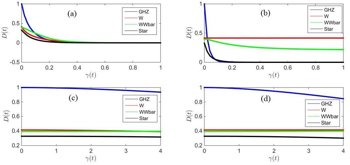
Figure 2: The dynamics of distribution of entanglement of pure states such as $|GHZ\rangle$,$|W\rangle$, $|W\bar{W}\rangle$ and $|Star\rangle$ in a dephasing environment are shown for (a) local Markov,(b) common Markov, (c) local Non-Markov and (d) common Non-Markov environments.

The entanglement distribution dynamics of the different pure states under a local Markovian environment is given in Fig. $2(a)$ and is represented in Eqs.(13)-(14). The entanglement distribution is maximum for GHZ states than for the rest of the pure states at $\gamma_{0}t=0$. As the system evolves we observe that the entanglement distribution decays monotonically to zero. From the plot Fig. $2(a)$, we can see that the the distribution of the GHZ state decays faster than that of the $W\bar{W}$ state. So we observe that in the range $0.1<\gamma_{0}t\leq 0.2$, the entanglement distribution is $D(|W\bar{W}\rangle)>D(|GHZ\rangle)>D(|W\rangle)>D(|Star\rangle)$.

In a common Markovian environment (i.e. Fig $2(b)$), the rate of decay of $D(t)$ is exponential. But the entanglement distribution of the W state remains constant with time. Meanwhile we observe that the distribution in the $W\bar{W}$ state decays with time but not as fast as the GHZ state. This decay of entanglement distribution of the GHZ state is because of the actual decay of the entanglement in the state. In the case of W state the entanglement distribution does not decay because this state has a decoherence free subspace. Finally we observe that the star states show a behaviour which is intermediate between that of the GHZ state and the $W\bar{W}$ state. In the long time limit, the entanglement distribution of the GHZ, star state and the $W\bar{W}$ decays to zero.

The entanglement distribution of some tripartite pure states does not decay in a local Non-Markovian dephasing environment. But from Fig.$2(c)$ and Fig.$2(d)$, we see that both in the case of a local and common Non-Markovian environment, the entanglement distribution of the GHZ state decays but only very slowly. So we observe that the entanglement distribution of the $W$, $W\bar{W}$ and star states are constant for both the local and common Non-Markovian dephasing environment, whereas distribution dynamics of the GHZ states change with the nature of the environment.

IV.2 Mixed states under dephasing environment

Sustainability of pure states are hard to be achieved from experimental view point. Keeping this in mind we have carried forward with our analysis on dynamics of distribution of entanglement, which has so far been studied in the case of pure tripartite states, to some mixed states that have been designed as mixtures of well-defined and significant tripartite states. In this regard, we have taken into consideration a few mixed states namely (i) Werner GHZ state, (ii) Werner W state and (iii) a mixture of GHZ and W states [53, 54, 55] shown below:

$$\rho^{wer}_{ghz}=p|GHZ\rangle\langle GHZ|+\frac{1-p}{8}\mathbb{I}_{8},$$ (15)

$$\rho^{wer}_{w}=p|W\rangle\langle W|+\frac{1-p}{8}\mathbb{I}_{8},$$ (16)

and

$$\rho^{ghz}_{w}=p|GHZ\rangle\langle GHZ|+(1-p)|W\rangle\langle W|.$$ (17)

Here, $p$ is the probability of mixture and $\mathbb{I}_{8}$ is the $8\times 8$ identity matrix. The states described in Eqs.(15) and (16), sometimes known as generalized Werner states where the mixtures of $|GHZ\rangle$ and $|W\rangle$ with completely unpolarized state (or maximally mixed state) have been taken respectively. Thus the two mixed states of eqs. (15) and (16) are mixtures of regular tripartite states with white noise. The third state described in eq.(17) is a statistical mixture of three way entangled GHZ state and a bipartite entangled W state. So the distribution depends on the relative proportion between these two types.

Distribution of entanglement of mixed states:

The dynamics of distribution of entanglement of the mixed states described in eqs.(15-17) subjected to dephasing environment is given below.

Tripartite mixed states $\rho^{wer}_{ghz}$ under Markovian and Non-Markovian dephasing

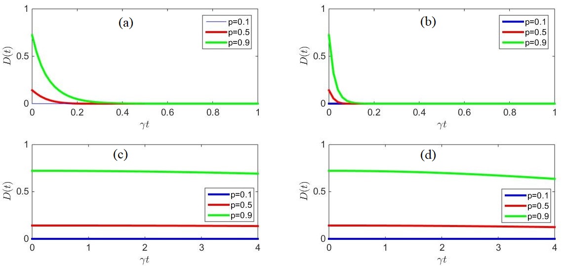
Figure 3: The dynamics of distribution of entanglement of mixed state $\rho^{wer}_{ghz}$ in a dephasing environment are shown for (a) local Markov,(b) common Markov, (c) local Non-Markov and (d) common Non-Markov environments.

The entanglement distribution of mixed states $\rho^{wer}_{ghz}$ described in Eq.(15) is given in Fig. $3$. In Fig. $3(a)$, the decay of entanglement distribution for a Werner-GHZ state is discussed for a local Markov dephasing environment. The decay of $D(t)$ is shown for the different values of the mixing parameter namely $p=0.1,0.5$ and $0.9$ respectively. The entanglement distribution decays monotonically for $p=0.9$ and $p=0.5$ respectively. In the case of $p=0.1$, the initial state is not entangled and since dephasing does not create entanglement the distribution is zero throughout. The decay of entanglement distribution in a Markov common bath exhibits the same features as the local bath, i.e., the distribtuion decays monotonically and in the long time limit it is zero. But the distribution falls much faster when the qubits are in contact with a common bath than when they are in a local bath. From Figs. $3(c)$ and $3(d)$, we observe the decay of entanglement distribution for both Non-Markovian local and common dephasing environment. The mixing parameter is chosen to be $p=0.9$ and for $p=0.5$, and the entanglement distribution falls, but very slowly for both these values of mixing parameter. This feature is present for both the local and common environments.

Tripartite mixed states $\rho^{wer}_{w}$ under Markovian and Non-Markovian dephasing

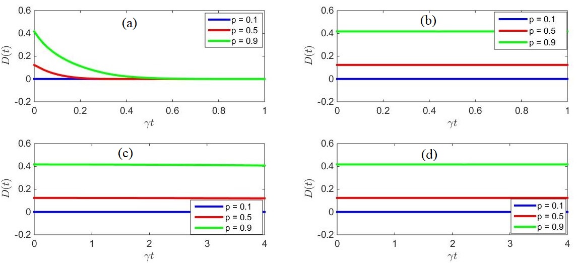
Figure 4: The dynamics of distribution of entanglement of mixed state $\rho^{wer}_{w}$ in a dephasing environment are shown for (a) local Markov,(b) common Markov, (c) local Non-Markov and (d) common Non-Markov environments.

In the case of the mixed states $\rho^{wer}_{w}$, the effect of the dephasing environment is as follows: For the local Markovian bath shown in Fig. $4(a)$, the distribution decays monotonically with time for $p=0.5$ and $p=0.9$. For $p=0.1$, there is no decay in the $Werner-W$ mixture. In the rest of the cases namely, the common Markovian bath Fig. $4(b)$, the local Non-Markovian bath Fig. $4(c)$ and the common Non-Markovian bath Fig. $4(d)$, the entanglement distribution remains constant throughout the evolution of the system. This is because the presence of a decoherence free subspace for the W-state.

Tripartite mixed states $\rho^{ghz}_{w}$ under Markovian and Non-Markovian dephasing

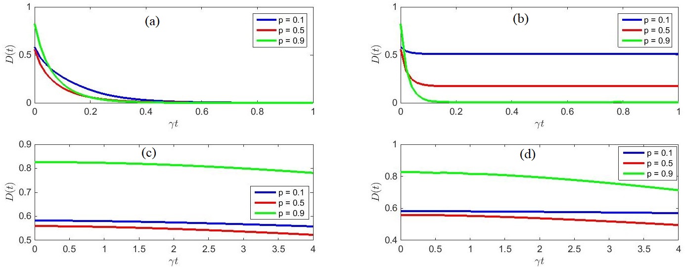
Figure 5: The dynamics of distribution of entanglement of mixed state $\rho^{ghz}_{w}$ in a dephasing environment are shown for (a) local Markov,(b) common Markov, (c) local Non-Markov and (d) common Non-Markov environments.

In this subsection we present the decay dynamics of the mixed state $\rho^{ghz}_{w}$ which is a mixture of GHZ and W states. The Markovian dynamics when the tripartite system are in contact with the local environments is given in Fig. $5(a)$. The distribution of entanglement decays monotonically with time and vanishes in the long time limit. The rate of decay depends on the value of the mixing parameter where we find that rate of decay is higher for higher values of $p$. This is because for higher values of $p$ the state has more GHZ state than W states and since GHZ states decay faster than W states. The Markovian dynamics of the $\rho^{ghz}_{w}$ in a common environment is shown in Fig. $5(b)$, where we observe that for $p=0.9$ when the state is predominantly GHZ it falls faster and reaches zero. In the situation where $p=0.5$, the distribtuion initially falls, but after a finite time it attains a saturation value, because while the distribution due to GHZ state goes to zero, the distribution due to the W state remains constant. The same behaviour is observed in the case where $p=0.1$, the only change is the saturation values is attained much faster than the GHZ state.

In Figs.$5(c)$ and $5(d)$, we see the dynamics of entanglement distribution for both local Non-Markovian and common Non-Markovina environments. For both these cases we find that distribution decays but very slowly with time. The rate of this decay is low for $p=0.1$ compared to when $p=0.9$ and $p=0.5$.

V Conclusion:

In the study of quantum information, it is always crucial to study the entanglement of the quantum states, since it is the key feature which is responsible for all the information proccessing tasks. When the quantum states are subjected to external environment, the quality of the states are affected by the environment. In the case of multipartite systems the environment might also affect the distribution of the entanglement. In our work we study the change in the distribution of the entanglement due to the external environment by investigating tripartite states. There are several measures available for computing the entanglement in bipartite systems. But for tripartite systems the only kind of measures we can use for both pure and mixed states is the distance based measures. In our work we use the relative entropy based measure of entanglement for finding the entanglement of the tripartite systems and the entanglement of the bipartite reduced states. Using these different entanglement measures we define the distribution of entanglement. To understand the effects of the environment we consider an external dephasing on the system. This dephasing environment, which arises from phase damping processes, is critical in describing decoherence in realistic systems with significant practical implications. The dynamics of distribution of entanglement of different tripartite pure and mixed states are analyzed. Additionally, we consider two distinct scenarios, (a) where each qubit is immersed in its own individual environment, and (b) all qubits share a common environment. Again we consider these two scenarios when the baths have either Markovian or Non-Markovian characteristics.

From the analysis of the distribution of entanglement for tripartite pure and mixed states in local as well as common environment, we observe that the three pure states viz $|GHZ\rangle$, $|W\bar{W}\rangle$ and $|Star\rangle$ exhibit decay of distribution of entanglement with time, only for the memoryless Markovian environment. The W-state decays during the Markovian dynamics only for the common environments. In the case of the Non-Markovian environment all the tripartite pure states do not exhibit decay due to an external dephasing environment irrespective of the fact whether they are in a Markovian or Non-Markovian environment. Thus the Non-Markovian environment has no effect on the transient dynamics of the entanglement distribution in tripartite pure states. The dynamics of tripartite mixed states like $Werner-GHZ$ ($\rho^{werner}_{ghz}$) states and $Werner-W$ ($\rho^{wer}_{w}$) states were also investigated to understand the effect of noise on the dephasing dynamics. The observation shows that the entanglement distribution remains constant throughout the evolution for Non-Markovian dynamics. We also consider the mixed state $\rho^{ghz}_{w}$ which is a mixture of the tripartite entangled GHZ states and bipartite entangled W states. In these states we find that the entanglement decay is proportional to the GHZ states in the mixture. From these results we conclude that $\it{(a)}$ The W states do not decay when they are in common environment and $\it{(b)}$ There is no decay of the distribution of entanglement for $|GHZ\rangle$, $|W\bar{W}\rangle$ and $|Star\rangle$, $\rho^{wer}_{ghz}$, $\rho^{wer}_{w}$ states in the Non-Markovian environment.

Declaration of competing interest The authors declare that they have no known competing financial interests or personal relationships that could have appeared to influence the work reported in this paper.

Data availability statement All data that support the findings of this study are included within the article (and any supplementary files).

References

- [1] Horodecki, R., Horodecki, P., Horodecki, M. and Horodecki K., Rev. of Mod. Phys., 81, 865, (2009).
- [2] Bennett, C.H., Brassard, G., Crépeau, C., Jozsa, R., Peres, A and Wootters, W. K., Phys. Rev. Lett., 70, 1895, (1993).
- [3] Bennett, C.H. and Wiesner, S.J., Phys. Rev. Lett., 69, 2881, (1992).
- [4] Gisin, N., Ribordy, G., Tittel, W. and Zbinden, H., Rev. Mod. Phys. 74, 145, (2002).
- [5] Nielsen, M. A. and Chuang, I. L., Quantum computation and quantum information, Cambridge University Press, (2010)
- [6] Zurek, W., Rev. Mod. Phys., 75, 715, (2003).
- [7] Breuer H.-P. and Petruccione F., Theory of Open Quantum Systems, Oxford University Press, 2002.
- [8] Steane, A. M., Phys. Rev. Lett., 77, 793, (1996).
- [9] Cory, D. G., Price, M., Maas, W., Knill, E., Laflamme, R., Zurek, W. H., Havel, T. F., and Somaroo, S. S., Phys. Rev. Lett., 81, 2152, (1998).
- [10] Zanardi, P., and Rasetti, M., Phys. Rev. Lett., 79, 3306, (1997).
- [11] Lidar, D. A., Chuang, I. L., and Whaley, K. B., Phys. Rev. Lett., 81, 2594, (1998).
- [12] Viola, L., Knill, E., and Lloyd, S., Phys. Rev. Lett., 82, 2417, (1999).
- [13] Viola, L., Llyod, S. and Knill, E., Phys. Rev. Lett., 83, 4888, (1999).
- [14] Braun, D., Phys. Rev. Lett., 89, 277901, (2002)
- [15] Sarlette, A., Raimon, J-M., Brune, M. and Rouchon, P., Phys. Rev. Lett., 107, 010402, (2011).
- [16] Nokkala, J., Galve, F., Zambrini, R., Maniscalco, S., and Pillo, J., Sci. Rep., 6. 26861, (2016).
- [17] Mazzola, L., Maniscalco, S., Pillo, J., Suominen, K. A., and Garraway, B. M., Phys. Rev. A, 79, 042302, (2009).
- [18] An, N. B., Kim, J., and Kim, K., Phys. Rev. A, 82, 032316, (2002).
- [19] Breuer, H.- P, Laine, E.-M, Pillo, J., and Vacchini, B., Rev. Mod. Phys., 88, 021002, (2002).
- [20] De. Vega, I., and Alonso, D., Rev. Mod. Phys., 89, 015001, (2017).
- [21] Bellomo, B., Franco, R. L., and Compagno, G., Phys. Rev. Lett., 99, 160502, (2007).
- [22] Wang, F.-Q, Zhang, Z.-M, and Liang, R.-S., Phys. Rev. A, 78, 062318, (2007).
- [23] Dajka, J., Mierzejewski, M., and Luczka, R.-S., Phys. Rev. A, 77, 042316, (2008).
- [24] Paz, J. P., and Roncaglia, A. J., Phys. Rev. Lett., 100, 220401, (2008).
- [25] Li, J.-G, Zou, J. , and Shao, B., Phys. Rev. A, 82, 042318, (2002).
- [26] Ali, M.-M, Chen, P.-W, and Goan, H.-S., Phys. Rev. A, 82, , 022103, (2010).
- [27] Weinstein, Y. S., Phys. Rev. A, 82, 032326, (2010).
- [28] San Ma, X., Wang, A. M., and Cao, Y., Phys. Rev. B, 76, 155327, (2007).
- [29] Aolita, L., Chaves, R., Cavalcanti, D., Acin, A., and Daviddovich, L., Phys. Rev. Lett., 100, 080501, (2008).
- [30] Lopez, C., Romero, G., Lastra, F., Solanko, E., and Re-Tamal, J. Phys. Rev. Lett., 101, 080503, (2008).
- [31] Weinstein, Y. S., Phys. Rev. A, 79, 012318, (2009).
- [32] Eltschka, C., Braun, D., and Siewert, J., Phys. Rev. A, 89, 062307, (2014).
- [33] Goan, H.-S., Jian, C.-C., and Chen, P.-W, Phys. Rev. A, 82, 012111, 2010.
- [34] Haikka, P., Johnson, T., and Maniscalco, S., Phys. Rev. A, 87, 010103, (2013).
- [35] Guarnieri, G., Smirne, A., and Vacchini, B., Phys. Rev. A, 90, 022110, (2014).
- [36] Wootters, W. K., Phys. Rev. Lett., 80, 2245.
- [37] Mintert, F., Kus, M., and Buchleitner, Phys. Rev. Lett., 95, 260502, (2005).
- [38] Coffman, V., Kundu, J., and Wootters, W. K., Phys. Rev. A, 61, 052306, (2000).
- [39] Wong, A., and Christensen, N., Phys. Rev. A, 63, 044301, (2001).
- [40] Vidal, G., and Werner, R. F., Phys. Rev. A, 65, 032314, (2002).
- [41] Lee, S., Chi, D.P., Oh, S.D., and Kim, J., Phys. Rev. A, 68, 062304, (2003).
- [42] Vedral, V., Plenio, M. B., Rippin, M. A.and Knight, P. L., Phys. Rev. Lett., 78, 2275, (1997).
- [43] Vedral, V., and Plenio, M. B., Phys. Rev. A, 57, 1619, (1998).
- [44] Vedral, V., Rev. Mod. Phys., 74, 1, (2002).
- [45] Leggett, A.J., Chakravarty, S., Dorsey, A. T., Fisher, M.P., Garg, A., and Zwerger, W., Rev. of Mod. Phys., 59,, 1, (1987).
- [46] Greenberger, D. M., Horne, M. A., and Zeilinger, A., Bell’s theorem, Quantum theory and conceptions of the universe, ed. M. Kafatos (Kluwer, Dordrecht, p.69), (1989).
- [47] Dr, W., and Cirac, J.I., Phys. Rev. A, 61, 042314, (2000).
- [48] Cao, H., Radhakrishnan, C., Ming, S., Ali, M.-M., Zhang, C., Huang, Y.-F, Byrnes, T., Li, C.-F., and Guo, G.-C., Phys. Rev. A, 102, 012403, (2020).
- [49] Dr, W., Vidal, G., and Cirac, J. I., Phys. Rev. A, 62, 062314, (2000).
- [50] Bouwmeester, D., Pan, J.-W., Daniell, M., Weinfurter, H., and Zeilinger, A., Phys. Rev. Lett., 82, 1345, (1999).
- [51] Yamamoto, T., Tamaki, K., Koashi, M., and Imoto, N., Phys. Rev. A, 66, 064301, (2002).
- [52] Roy, S., Bhattacharjee, A., Radhakrishnan, C., Ali, M.-M., and Ghosh, B., Int. Jour. Quant. Inf., 21, 2, (2023).
- [53] Jung, E., Hwang, M.-R, Park, D., and Son, J.-W., Phys. Rev. A, 79, 024306, (2009).
- [54] Lohmayer, R., Osterloh, A., Siewart, J., and Uhlmann, A., Phys. Rev. Lett., 97, 260502, (2006).
- [55] Czerwinski, A., Int. Jour. Mod. Phys. B, 36, 19, (2022).