Obliquities of Exoplanet Host Stars

Measurements of the obliquities in exoplanet systems have revealed some remarkable architectures, some of which are very different from the Solar System. Nearly 200 obliquity measurements have been obtained through observations of the Rossiter-McLaughlin (RM) effect. Here we report on observations of 19 planetary systems that led to 17 clear detections of the RM effect and 2 less secure detections. After adding the new measurements to the tally, we use the entire collection of RM measurements to investigate four issues that have arisen in the literature. i) Does the obliquity distribution show a peak at approximately 90^∘? We find tentative evidence that such a peak does exist when restricting attention to the sample of sub-Saturn planets and hot Jupiters orbiting F stars. ii) Are high obliquities associated with high eccentricities? We find the association to be weaker than previously reported, and that a stronger association exists between obliquity and orbital separation, possibly due to tidal obliquity damping at small separations. iii) How low are the lowest known obliquities? Among hot Jupiters around cool stars, we find the dispersion to be $1.4\pm 0.7^{\circ}$, smaller than the 6^∘ obliquity of the Sun, which serves as additional evidence for tidal damping. iv) What are the obliquities of stars with compact and flat systems of multiple planets? We find that they generally have obliquities lower than $10^{\circ}$, with several remarkable exceptions possibly caused by wide-orbiting stellar or planetary companions.

1 Introduction

Hot Jupiters, planets on extremely eccentric orbits, planets orbiting binary stars, planets orbiting white dwarfs and neutron stars — these and other types of exotic planetary systems have been discovered over the last 30 years. A diversity of architectures has also been revealed by measurements of the host star’s obliquity, i.e., the angle between the star’s spin axis and a planet’s orbital axis, or at least its sky projection. Thanks to many research groups pursuing these measurements, usually by means of the Rossiter-McLaughlin (RM) effect, we now have a sample of nearly 200 measurements including prograde, polar, and retrograde orbits (see, e.g., Albrecht et al., 2022, for a review).

Table 1: Systems observed and spectroscopic observations.

Target	$V$	Instrument	ID	Night	$N$	$t$/$\Delta t$	$T_{41}$
	(mag)			(dd-mm-yyyy)		(s)	(hr)
HD 118203 b	8.14	FIES	60-417	24-03-2020	12	900/1170	5.64
HD 118203 b	8.14	FIES	65-851	18-06-2022	21	600/768	5.64
HD 148193 b	9.77	HARPS-N	A43TAC_11	15-06-2021	23	1140/1168	6.61
K2-261 b	10.61	HARPS-N	A44TAC_16	24-03-2022	40	600/625	5.11
K2-287 b	11.41	ESPRESSO	105.20KD.003	05-07-2021	26	540/600	3.42
KELT-3 b	9.87	FIES	65-851	08-04-2022	15	900/1080	3.15
KELT-4Ab	9.5	FIES	62-506	27-01-2021	16	900/1090	3.46
LTT 1445Ab	11.22	HARPS-N	A41TAC_19	05-09-2020	15	900/920	1.38
TOI-451Ab	11.02	ESPRESSO	109.22Z4.002	24-09-2022	21	720/755	2.04
TOI-813 b	10.32	ESPRESSO	109.22Z4.008	19-01-2023	29	800/832	13.10
TOI-892 b	11.45	HARPS-N	A44TAC_16	01-01-2022	21	960/987	5.51
TOI-1130 c	11.37	ESPRESSO	105.20KD.002	01-06-2021	23	660/700	2.02
WASP-50 b	11.44	ESPRESSO	109.22Z4.007	23-07-2022	61	240/270	1.81
WASP-59 b	12.78	HIRES	N117Hr	23-11-2016	20	787/835	2.45
WASP-136 b	9.98	FIES	63-505	30-08-2021	20	1140/1320	5.57
WASP-148 b	12.25	HARPS-N	A42TAC_22	21-03-2021	17	900/920	3.14
WASP-172 b	11.0	ESPRESSO	109.22Z4.006	01-06-2022	31	900/940	5.47
WASP-173Ab	11.3	ESPRESSO	109.22Z4.003	23-07-2022	34	555/590	2.33
WASP-186 b	10.82	FIES	64-506	11-10-2021	15	900/1080	2.75
XO-7 b	10.52	FIES	65-851	27-08-2022	12	840/1000	2.77

• In the columns we list the Johnson $V$ magnitudes, the instrument used, the program IDs, the dates of the observation nights, the number of exposures on a given night ($N$), the exposure duration ($t$), sampling time ($\Delta t$), and the total transit duration ($T_{41}$).

Here we present observations of 19 transiting exoplanets aiming to detect the RM effect and measure the sky-projected stellar obliquities. Together with the sample drawn from the literature, we also wanted to investigate four issues regarding the distribution of obliquities.

1. For most systems in the sample, the projected obliquity ($\lambda$) is known but not the obliquity itself ($\psi$) because of missing information about the inclination of the stellar rotation axis with respect to the line of sight ($i_{\star}$). Using the subset of 57 systems for which $\psi$ has been measured, Albrecht et al. (2021) found evidence for a preponderance of perpendicular planets, i.e., a peak in the obliquity distribution near $90^{\circ}$. Following up on this result, Siegel et al. (2023) and Dong & Foreman-Mackey (2023) applied more advanced statistical techniques that allowed the entire sample to be used, and did not find evidence for a peak. With an enlarged sample, we wanted to revisit this issue and see whether there is a particular category of planets for which a peak does exist.

2. Three theories have been proposed to explain the existence of hot Jupiters: in-situ formation, disk-driven migration, and high-eccentricity or tidally-driven migration (see Dawson & Johnson, 2018, for a review). The latter process would not only increase the orbit’s eccentricity but might also raise its inclination relative to the star’s equatorial plane. One might therefore expect high eccentricities and obliquities to be statistically associated, and evidence for such an association has been reported (Rice et al., 2022a). After noticing some errors in this earlier study, we decided to revisit the issue with an enlarged sample.

3. Stars with $T_{\rm eff}\lesssim 6{,}250$ K that host hot Jupiters tend to have especially low obliquities. Indeed, the most precise such measurements ($\sigma_{\lambda}<2^{\circ}$) show an obliquity dispersion less than one degree — smaller than 6.2^∘ obliquity of the Sun relative to the Solar System’s invariable plane. Highlighting this result, Albrecht et al. (2022) interpreted the very low obliquities of hot Jupiters around cool stars as evidence for tidal obliquity damping. If this is true, then by continuing to perform precise measurements, we might gain a better understanding of the evolution of hot Jupiters and rates of tidal dissipation. With the enlarged sample, we wanted to see if this trend still holds and include the numerous but less precise obliquity measurements in the determination of the dispersion.

4. The first five measurements of $\lambda$ for stars with compact multiple-transiting planetary systems (“multis”) were all consistent with low obliquities (Albrecht et al., 2013), following the blueprint of the Solar System. Since then, several exceptions have been discovered (Hjorth et al., 2021; Huber et al., 2013; Chaplin et al., 2013). The misalignments in these cases are suspected of being caused by the effects of an outer massive companion. We wanted to assess the obliquity distribution of the multis, and see whether all of the misaligned multis have outer companions.

The paper is structured as follows. Section 2 describes the general characteristics of the new data. Section 3 presents our general approach to analyzing the data, and Section 4 discusses the particulars for each of the 19 observed systems. Section 5 discusses the issues and questions posed above, and Section 6 summarizes our conclusions.

2 Observations

To measure the projected obliquity of each host star, we performed high-resolution optical spectroscopy over a time range (typically 4–8 hours) spanning a planetary transit and tried to detect the RM effect. Table 1 gives the names of the 19 systems, the names of the telescopes and instruments employed, and some key observational characteristics. The telescopes and instruments are further described in Table 2. Tables 3 and 4 give some of the basic parameters of the host stars and their planets. Table 13 provides all of the apparent radial velocity (RV) measurements. These spectroscopic data were supplemented by the best available transit light curves, as described below.

Table 2: Telescopes and spectrographs used in this study.

Telescope	Aperture	Instrument	$R$	$\sigma_{\mathrm{PSF}}$
	(m)			(km s-1)
NOT	2.56	FIES	67 000	1.9
TNG	3.6	HARPS-N	115 000	1.1
VLT	8.2	ESPRESSO	140 000	0.9
Keck-1	10	HIRES	70 000	1.8

• $R$ is the resolution and $\sigma_{\mathrm{PSF}}$ the width of the point spread function in velocity units.

2.1 Spectroscopy

Seven systems were observed with the Echelle SPectrograph for Rocky Exoplanets and Stable Spectroscopic Observations (ESPRESSO; Pepe et al., 2021) that can be fed by any of the four Very Large Telescopes at Paranal Observatory, Chile. Another seven systems were observed with the FIber-fed Echelle Spectrograph (FIES; Frandsen & Lindberg, 1999; Telting et al., 2014) mounted on the Nordic Optical Telescope (NOT; Djupvik & Andersen, 2010) located on the Roque de los Muchachos, La Palma, Spain. For five systems, we used the High Accuracy Radial velocity Planet Searcher for the Northern hemisphere (HARPS-N; Cosentino et al., 2014) mounted on the Telescopio Nazionale Galileo (TNG), also on the Roque de los Muchachos. For one system, we used the High Resolution Echelle Spectrometer (HIRES; Vogt et al., 1994) mounted on the 10-m Keck-1 telescope on Mauna Kea, Hawai’i, USA.

The data from ESPRESSO and HARPS-N were reduced and radial velocities (RVs) were obtained using the standard data reduction software (DRS; Lovis & Pepe, 2007; Pepe et al., 2021; Dumusque et al., 2021). The FIES data for all but two systems were reduced using FIEStool, and RVs were extracted using FIESpipe following an approach similar to that described by Zechmeister et al. (2018). The FIES observations of WASP-136 and WASP-186 were reduced and RVs extracted following the procedure described by Gandolfi et al. (2015). To account for any instrumental RV drift of the FIES spectrograph, we observed the spectrum of a Thorium-Argon (ThAr) lamp in between each science exposure. The HIRES spectra were obtained with the iodine cell in the light path, and the RV extraction followed the standard HIRES forward modelling pipeline of the California Planet Search (CPS; Howard et al., 2010) using the methodology of Butler et al. (1996).

For some systems, in addition to the apparent RVs we modeled the shape of the Cross Correlation Function (CCF) of the absorption lines. For the ESPRESSO and HARPS-N data, we used the CCFs that are automatically produced by the standard reduction pipelines. For the FIES data, we derived CCFs using a template spectrum based on the most suitable model atmosphere from the library of Castelli & Kurucz (2003), as implemented in FIESpipe.

2.2 Photometry

Light curves of all 19 of the systems are available from the databases of either the K2 mission (Howell et al., 2014) or the Transiting Exoplanet Survey Satellite (TESS; Ricker et al., 2015). For the K2 data, we used the light curves from the EVEREST pipeline (Luger et al., 2016, 2018). The TESS data were downloaded and extracted using the lightkurve package (Lightkurve Collaboration et al., 2018), and the RegressionCorrector was applied to reduce the systematic variations due to scattered light. Our parametric model for each system was based on jointly fitting the photometric and spectroscopic data. In some cases, we supplemented the space-based photometry with ground-based photometry to refine the transit ephemerides.

Table 3: Key literature orbital and planetary parameters.

Planet	$P$	$e$	$a/R_{\star}$	$R_{\rm p}/R_{\star}$	$b$	$M_{\mathrm{p}}$	$R_{\mathrm{p}}$
	(d)					(MJ)	(RJ)
HD 118203 b	$6.13499(3)$	$0.314\pm 0.017$	$7.23^{+0.13}_{-0.14}$	$0.05552^{+0.00017}_{-0.00019}$	$0.111^{+0.076}_{-0.095}$	$2.17^{+0.07}_{-0.08}$	$1.14\pm 0.03$
HD 148193 b	$20.38084(2)$	$0.13_{-0.09}^{+0.12}$	$20.2\pm 0.5$	$0.0462^{+0.0008}_{-0.0005}$	$0.31^{+0.19}_{-0.21}$	$0.092\pm 0.015$	$0.764^{+0.018}_{-0.017}$
K2-261 b	$11.63344(12)$	$0.42\pm 0.03$	$13.38^{+0.16}_{-0.18}$	$0.05178^{+0.0006}_{-0.0005}$	$0.187$	$0.22\pm 0.03$	$0.85^{+0.03}_{-0.02}$
K2-287 b	$14.89329(3)$	$0.48\pm 0.03$	$23.9^{+0.3}_{-0.3}$	$0.0801^{+0.0010}_{-0.0009}$	$0.779$	$0.32\pm 0.03$	$0.833\pm 0.013$
KELT-3 b	$2.7033904(10)$	$0$	$6.0\pm 0.2$	$0.0939\pm 0.0011$	$0.606^{+0.037}_{-0.046}$	$1.47\pm 0.07$	$1.35\pm 0.07$
KELT-4Ab	$2.989594(5)$	$0.03^{+0.03}_{-0.02}$	$5.8\pm 0.2$	$0.1089\pm 0.0005$	$0.689^{+0.011}_{-0.012}$	$0.90\pm 0.06$	$1.70\pm 0.05$
LTT 1445Ab	$5.358766(4)$	$<0.110$	$30.9^{+1.1}_{-1.2}$	$0.0451^{+0.0014}_{-0.0013}$	$0.17^{+0.15}_{-0.12}$	$0.0090\pm 0.0008$	$0.116^{+0.006}_{-0.005}$
TOI-451Ab	$1.85870(3)$	$0$	$6.93^{+0.11}_{-0.16}$	$0.0199^{+0.0010}_{-0.0011}$	$0.22^{+0.20}_{-0.15}$	…	$0.170\pm 0.011$
TOI-813 b	$83.891\pm 0.003$	…	$47.2^{+2.1}_{-3.8}$	$0.03165^{+0.00072}_{-0.00061}$	$0.30^{+0.18}_{-0.19}$	…	$0.60\pm 0.03$
TOI-892 b	$10.62656(7)$	$<0.125$ a	$14.2^{+0.8}_{-0.7}$	$0.0790\pm 0.0010$	$0.43^{+0.09}_{-0.13}$	$0.95\pm 0.07$	$1.07\pm 0.02$
TOI-1130 c	$8.35038(3)$	$0.047^{+0.040}_{-0.027}$	$22.21^{+0.50}_{-0.43}$	$0.218^{+0.037}_{-0.029}$	$0.995^{+0.046}_{-0.043}$	$0.97\pm 0.04$	$1.5^{+0.3}_{-0.2}$
WASP-50 b	$1.955096(5)$	$0.009^{+0.011}_{-0.006}$	$7.51^{+0.17}_{-0.15}$	$0.1404\pm 0.0013$	$0.687^{+0.014}_{-0.016}$	$1.47\pm 0.09$	$1.15\pm 0.05$
WASP-59 b	$7.919585(10)$	$0.100\pm 0.042$	$24\pm 2$	$0.130\pm 0.006$	$0.29\pm 0.18$	$0.863\pm 0.045$	$0.775\pm 0.068$
WASP-136 b	$5.215357(6)$	$0$	$6.87\pm 0.12$	$0.064\pm 0.012$	$0.59^{+0.08}_{-0.14}$	$1.51\pm 0.08$	$1.38\pm 0.16$
WASP-148 b	$8.80381(4)$	$0.220\pm 0.063$	$19.8\pm 1.5$	$0.0807\pm 0.0007$	$0.05\pm 0.07$	$0.29\pm 0.03$	$0.72\pm 0.06$
WASP-172 b	$5.477433(7)$	$0$	$8.0\pm 0.5$	$0.085\pm 0.014$	$0.45\pm 0.12$	$0.47\pm 0.10$	$1.57\pm 0.10$
WASP-173Ab	$1.3866532(3)$	$0$	$4.78\pm 0.17$	$0.111\pm 0.014$	$0.40\pm 0.08$	$3.69\pm 0.18$	$1.20\pm 0.06$
WASP-186 b	$5.026799(13)$	$0.33\pm 0.01$	$8.78\pm 0.18$	$0.078\pm 0.017$	$0.84^{+0.01}_{-0.02}$	$4.22\pm 0.18$	$1.11\pm 0.03$
XO-7 b	$2.864142(4)$	$0.04\pm 0.03$	$6.43\pm 0.14$	$0.0953\pm 0.0009$	$0.71\pm 0.02$	$0.71\pm 0.03$	$1.37\pm 0.03$

• In the period column, the number in parentheses is the uncertainty in the last digit of the period.

• Sources are given in Table 4 for the corresponding host.

• With 98% confidence.

3 Data analysis

3.1 Photometric data

The photometric data provide tight constraints on the orbital period ($P$), the time of conjunction of a transit chosen to be the reference epoch, ($T_{0}$), the planet-to-star radius ratio ($R_{\rm p}/R_{\star}$), the cosine of the orbital inclination ($\cos i$), and the ratio of the semi-major axis and stellar radius ($a/R_{\star}$). Uniform prior probability distributions were adopted for these parameters.

To model the stellar limb darkening function, we used a standard quadratic law and allowed the sum of the two coefficients (the center-to-limb intensity ratio) to be an adjustable parameter, while holding the difference fixed at the value obtained from the tables of Claret et al. (2013); Claret (2018) as appropriate for the photometric bandpass and the star’s effective temperature ($T_{\rm eff}$), surface gravity ($\log g$), and metallicity ($[\rm Fe/H]$). See Table 5 and Table 7 for details. The sum of coefficients was subjected to a Gaussian prior with a width of $0.1$ and a central value from the aforementioned tables.

In cases for which a nonzero orbital eccentricity has been reported (HD 118203 b, K2-261 b, K2-287 b, WASP-148 b, and WASP-186 b), we applied Gaussian priors on $e$ and the argument of periastron ($\omega$) using the values given in Table 3. For the multis, we applied Gaussian priors on the parameters of all planets apart from the transiting planet that was the target of our observations. The main effect of these planets on our model is to change the slope of the RV time series on the night of the transit that was observed spectroscopically. When two planets are transiting simultaneously, the shape of the transit light curve is also affected. Simultaneous transits occasionally occurred (for TOI-1130 and TOI-451A) within the long intervals spanned by the photometric data, but did not occur during any of our 19 spectroscopic observations.

Table 4: Key literature stellar parameters.

Star	$T_{\rm eff}$	$\log g$	$[\rm Fe/H]$	$M_{\star}$	$R_{\star}$	Age	Source
	(K)	(cgs; dex)	(dex)	(M⊙)	(R⊙)	(Gyr)
HD 118203	$5683\pm 85$	$3.889\pm 0.018$	$0.223\pm 0.076$	$1.13^{+0.05}_{-0.06}$	$2.10\pm 0.05$	$5.32^{+0.96}_{-0.73}$	1
HD 148193	$6198\pm 100$	$4.18\pm 0.10$	$-0.13\pm 0.06$	$1.23^{+0.02}_{-0.05}$	$1.63^{+0.03}_{-0.02}$	$3.5^{+1.3}_{-0.5}$	2
K2-261	$5537\pm 71$	$4.21\pm 0.11$	$0.36\pm 0.06$	$1.105\pm 0.019$	$1.669\pm 0.022$	$8.8^{+0.4}_{-0.3}$	3
K2-287	$5695\pm 58$	$4.398\pm 0.015$	$0.20\pm 0.04$	$1.06\pm 0.02$	$1.070\pm 0.010$	$4.5\pm 1$	4
KELT-3	$6306\pm 50$	$4.21\pm 0.03$	$0.04\pm 0.08$	$1.28\pm 0.06$	$1.47\pm 0.07$	$3\pm 0.2$	5
KELT-4A	$6207\pm 75$	$4.11\pm 0.03$	$0.12\pm 0.07$	$1.20^{+0.07}_{-0.06}$	$1.60\pm 0.04$	$4.44^{+0.78}_{-0.89}$	6
LTT 1445A	$3340\pm 150$	$5.0$	$-0.34\pm 0.09$	$0.257\pm 0.014$	$0.265^{+0.011}_{-0.010}$	…	7
TOI-451A	$5550\pm 56$	$4.53$	$0.0$	$0.95\pm 0.02$	$0.88\pm 0.03$	$0.125\pm 0.008$	8
TOI-813	$5907\pm 150$	$3.86\pm 0.14$	$0.10\pm 0.10$	$1.32\pm 0.06$	$1.94\pm 0.10$	$3.73\pm 0.62$	9
TOI-892	$6261\pm 80$	$4.26\pm 0.02$	$0.24\pm 0.05$	$1.28\pm 0.03$	$1.39\pm 0.02$	$2.2\pm 0.5$	10
TOI-1130	$4250\pm 67$	$4.60\pm 0.02$	$>0.2$	$0.684^{+0.016}_{-0.017}$	$0.687\pm 0.015$	$8.2^{+3.8}_{-4.9}$	11
WASP-50	$5400\pm 100$	$4.5\pm 0.1$	$-0.12\pm 0.08$	$0.89^{+0.08}_{-0.07}$	$0.84\pm 0.03$	$7\pm 3.5$	12
WASP-59	$4650\pm 150$	$4.55\pm 0.15$	$-0.15\pm 0.11$	$0.72\pm 0.04$	$0.61\pm 0.04$	$0.5^{+0.7}_{-0.4}$	13
WASP-136	$6250\pm 100$	$3.9\pm 0.1$	$-0.18\pm 0.10$	$1.41\pm 0.07$	$2.2\pm 0.2$	$3.62\pm 0.70$	14
WASP-148	$5460\pm 130$	$4.40\pm 0.15$	$0.11\pm 0.08$	$1.00\pm 0.08$	$1.03\pm 0.20$	…	15
WASP-172	$6900\pm 150$	$4.1\pm 0.2$	$-0.10\pm 0.08$	$1.49\pm 0.07$	$1.91\pm 0.10$	$1.79\pm 0.28$	16
WASP-173A	$5700\pm 150$	$4.5\pm 0.2$	$0.16\pm 0.14$	$1.05\pm 0.08$	$1.11\pm 0.05$	$6.78\pm 2.93$	17
WASP-186	$6300\pm 100$	$4.1\pm 0.2$	$-0.08\pm 0.14$	$1.21^{+0.07}_{-0.08}$	$1.46\pm 0.02$	$3.1^{+1.0}_{-0.8}$	18
XO-7	$6250\pm 100$	$4.25\pm 0.02$	$0.43\pm 0.06$	$1.405\pm 0.059$	$1.480\pm 0.022$	$1.18^{+0.98}_{-0.71}$	19

• The sources refer to the following references: 1 Pepper et al. (2020), 2 Chontos et al. (2024), 3 Johnson et al. (2018), 4 Jordán et al. (2019), 5 Pepper et al. (2013), 6 Eastman et al. (2016), 7 Winters et al. (2022), 8 Newton et al. (2021), 9 Eisner et al. (2020), 10 Brahm et al. (2020), 11 Huang et al. (2020), 12 Gillon et al. (2011), 13 Hébrard et al. (2013), 14 Lam et al. (2017), 15 Hébrard et al. (2020), 16 Hellier et al. (2019a), 17 Hellier et al. (2019a), 18 Schanche et al. (2020), 19 Crouzet et al. (2020).

We modeled the light curves using the batman package (Kreidberg, 2015), which is based on the equations of Mandel & Agol (2002). In addition to accounting for the transit and white noise in the measurements, we included a Gaussian process (GP) using celerite (Foreman-Mackey et al., 2017). We generally employed a Matérn-3/2 kernel, which is characterised by two hyperparameters: the amplitude ($A$) and the timescale ($\tau$). For the time series with 30-minute sampling, evenly spaced model light curves were created and integrated over to mimic a cadence of 2 min.

Table 5: Limb-darkening coefficients and velocity fields.

	$q_{1}$/$q_{2}$	$q_{1}$/$q_{2}$	$q_{1}$/$q_{2}$	$\zeta_{\star}$	$\xi_{\star}$
	TESS	K2	$V$	(km s-1)
HD 118203	0.30/0.28	…	0.31/0.20	4.11	1.00
HD 148193	0.23/0.31	…	0.49/21	5.23	1.31
K2-261	0.41/0.22	0.54/0.15	0.58/0.16	2.20	1.30
K2-287	0.53/0.17a	0.38/0.19	0.58/0.16	2.76	0.92
KELT-3	0.23/0.31	…	0.47/0.23	5.45	1.39
KELT-4A	0.23/0.31	…	0.50/0.21	5.23	1.31
LTT 1445A	0.17/0.44	…	0.70/0.07	1	0.9
TOI-451A	0.35/0.25	…	0.57/0.16	2.60	0.95
TOI-813	0.26/0.30	…	0.52/0.20	4.73	1.12
TOI-892	0.24/0.30	…	0.44/0.24	5.17	1.35
TOI-1130	0.51/0.17	…	0.49/0.25	3.59	0.90
WASP-50	0.35/0.25	…	0.62/0.14	2.49	0.90
WASP-59	0.48/0.17	0.68/0.07b	0.72/0.06	2.90	0.83
WASP-136	0.23/0.31	…	0.45/0.21	5.89	1.35
WASP-148	…	…	0.62/0.14	2.75	0.92
WASP-172	0.18/0.33	…	0.42/0.27	6.0	1.5
WASP-173A	0.31/0.27	…	0.54/0.18	3.28	1.04
WASP-186	0.23/0.31	…	0.44/0.23	5.75	1.43
XO-7	0.25/0.32	…	0.49/0.21	5.2	1.34

• The second, third, and fourth columns show the $q_{1}$ and $q_{2}$ quadratic limb darkening pairs we used as priors in the TESS, K2, and spectrograph bands. For the latter we simply assumed the $V$-filter. We obtained these using values for $T_{\rm eff}$, $\log g$, and $[\rm Fe/H]$ in tabulated in Table 4 and we queried the limb-darkening tables for the quadratic law by Claret et al. (2013, for K2 and $V$) and Claret (2018, for TESS). The macro- ($\zeta_{\star}$) and micro-turbulence ($\xi_{\star}$) priors were obtained from the relations in Doyle et al. (2014) and Bruntt et al. (2010), respectively, again using the values from Table 4, with the exception of WASP-172 and LTT 1445A (see Section 3).

• These values are for CHEOPS and not TESS. Queried from Claret (2021).

• These values are for the $r^{\prime}$ passband and not K2. Queried from Claret et al. (2012).

3.2 Stellar rotation

The analysis of the RM effect is aided by knowledge of the stellar rotation velocity or period. We tried to use the available spectroscopic and photometric data to measure these quantities independently of the transit data, as describe below.

3.2.1 Projected rotation velocity

The amplitude of the RM effect scales with $v\sin i_{\star}$, the product of the stellar rotation speed and the sine of the line-of-sight inclination of the stellar spin axis. Therefore, knowing $v\sin i_{\star}$ helps to plan observations and analyze the results. When the RM effect is detected with a high signal-to-noise ratio (SNR), $v\sin i_{\star}$ can be determined precisely from the RM data. Indeed, for stars with a high obliquity, the effects of differential rotation might be detectable (Gaudi & Winn, 2007; Cegla et al., 2016a).

Table 6: Stellar rotation parameters.

	$v\sin i_{\star}$		$P_{\rm rot}$
	(km s-1)		(d)
Star	Literature	This work	Literature	This work
HD 118203	$4.7$	$4.9\pm 0.4$	…	$6.1\pm 0.4$
HD 148193	$5.9\pm 1.0$	$6.27\pm 0.02$	…	…
K2-261	$3.70\pm 0.17$	$1.59\pm 0.17$	…	…
K2-287	$3.2\pm 0.2$	$1.99\pm 0.02$	…	…
KELT-3	$10.2\pm 0.5$	$7.59\pm 0.16$	…	…
KELT-4A	$6.2\pm 1.2$	$6.0\pm 0.4$	…	…
LTT 1445A	$<3.4$	$1.41\pm 0.11$	…	…
TOI-451A	$7.9\pm 0.5$	$8.16\pm 0.02$	$5.1\pm 0.1$	$5.3\pm 0.5$
TOI-813	$8.2\pm 0.9$	$8.33\pm 0.02$	…	…
TOI-892	$7.69\pm 0.5$	$6.2\pm 0.5$	…	…
TOI-1130	$4.0\pm 0.5$	$1.28\pm 0.05$	…	…
WASP-50	$2.6\pm 0.5$	$1.40\pm 0.12$	$16.3\pm 0.5$	…
WASP-59	$2.3\pm 1.2$	…	…	…
WASP-136	$13.1\pm 0.8$	$12.06\pm 0.04$	…	$5.4\pm 0.5$
WASP-148	$3\pm 2$	$2.0\pm 0.4$	$26.2\pm 1.3$	$26\pm 4$
WASP-172	$13.7\pm 1.0$	$13.33\pm 0.05$	…	$7.0\pm 0.7$
WASP-173A	$6.1\pm 0.3$	$6.62\pm 0.06$	$7.9\pm 0.1$	$8.4\pm 1.1$
WASP-186	$15.6\pm 0.9$	$14.8\pm 0.2$	…	$4.8\pm 1.9$
XO-7	$6\pm 1$	$5.2\pm 0.3$	…	$3.62\pm 0.12$

• Measurements of $v\sin i_{\star}$ and $P_{\mathrm{rot}}$ from the literature (see Table 4 for citations) and those derived in this work. The uncertainties reported for $v\sin i_{\star}$ generally refer to statistical uncertainties or the scatter in results of analyzing different spectra. Because they do not include systematic uncertainties, we imposed a minimum uncertainty of $0.5$ km s^-1 in our analysis.

In more typical cases in which the RM effect is detected with a modest SNR, it is useful to determine $v\sin i_{\star}$ by modeling the spectral line broadening outside of transits, and thereby gain the option of applying a prior constraint on $v\sin i_{\star}$ when modeling the RM effect. For this purpose, we used the broadening function (BF) method of Rucinski (1999) as implemented in FIESpipe, which is based on an appropriate model atmosphere from Castelli & Kurucz (2003). The BFs were created from high SNR orders from out-of-transit spectra, where we visually inspected the result to ensure that the BF created from a given order was well-behaved. This typically meant selecting central orders typically with wavelengths $\sim$5000-6000 Å. Orders containing telluric lines were excluded. For a given epoch we stacked the BFs from the individual orders to create the highest possible SNR BF for that epoch. We applied this method not only to the FIES spectra but also the ESPRESSO and HARPS-N spectra. To extract $v\sin i_{\star}$ we fitted the theoretical rotational BF from Kaluzny et al. (2006, Eq. (2)). The model includes the rotational broadening parameters along with a parameter representing non-rotational broadening (in most cases dominated by the finite instrumental resolution).

Table 6 gives the results. The tabulated $v\sin i_{\star}$ is the median of the best-fit results of analyzing spectra from different epochs, and the tabulated uncertainty is the standard deviation between those epochs, which in most cases are unrealistically small. This is especially true for observations where we only have few out-of-transit observations. For systems where we only had two out-of-transit spectra, we used the first ingress as a third spectrum. Our measurements are generally in agreement with previously published results. The most significant deviations are seen for the most slowly-rotating stars, where the details of extracting line profiles and modeling non-rotational broadening are most important. When modeling the RM effect, we imposed Gaussian priors based on our $v\sin i_{\star}$ determinations, with a minimum width of $\sigma=0.5$ km s^-1 to account for possible systematic errors.

To test if our choice of the width of the uncertainty interval in the $v\sin i_{\star}$ prior does significantly affect our results for the projected obliquity, we selected four systems in our sample for which we expect the result of lambda to be most sensitive to $v\sin i_{\star}$ (low impact parameter, incomplete transit coverage) and performed the same analysis as described below. However, now with an uncertainty in $v\sin i_{\star}$ of 1.0 km s^-1. In all four cases we find that the highest probability value for $\lambda$ changes only by a small fraction of its uncertainty interval, relative to the 0.5 km s^-1 case.

3.2.2 Photometric rotation period

We attempted to measure the rotation period ($P_{\mathrm{rot}}$) by seeking periodicities in the K2 and TESS light curves. The combination of the rotation period, $v\sin i_{\star}$, and $R_{\star}$ can be used to constrain the stellar inclination (Masuda & Winn, 2020), which in turn can be used in combination with $i_{\rm orb}$ and $\lambda$ to determine the “true” or three-dimensional obliquity.

We used the method based on the auto-correlation function (ACF) described by McQuillan et al. (2014). After removing the data affected by transits, we searched for peaks in the ACF as a function of lag. When multiple peaks were seen, we fitted a linear function between peak number and lag, the slope of which is an estimate of the rotation period (e.g., Hjorth et al., 2021).

Table 6 gives the results. Empty entries mark the cases for which no period could be determined. For two systems, TOI-813 and TOI-892, peaks were seen in the ACF (corresponding to periods of $10.1\pm 0.6$ d and $2.76\pm 0.11$ d, respectively), but because the statistical significance was weak, the results do not appear in Table 6. For WASP-50, a series of strong peaks seemed to imply a period of $7.2\pm 1.8$ d, which contrasts with the value of $16.3\pm 0.5$ d reported by Gillon et al. (2011). They also noted that the true rotation period could be 32.6 days if there are similar spot patterns on opposite stellar hemispheres. We folded the light curve using trial periods of $16.3$ d or $32.6$ d but neither choice seemed compelling. Evidently, the variability of WASP-50 is complex, which is why Table 6 contains no entry for WASP-50.

We note that the estimated rotation periods of WASP-136 and WASP-186, $5.4\pm 0.5$ d and $4.8\pm 1.9$ d, are both close to the orbital period of the transiting planets. These systems might have been driven into spin-orbit synchronization by tidal interactions between the planet and star (e.g., Albrecht et al., 2012b; Brown, 2014; Penev et al., 2018).

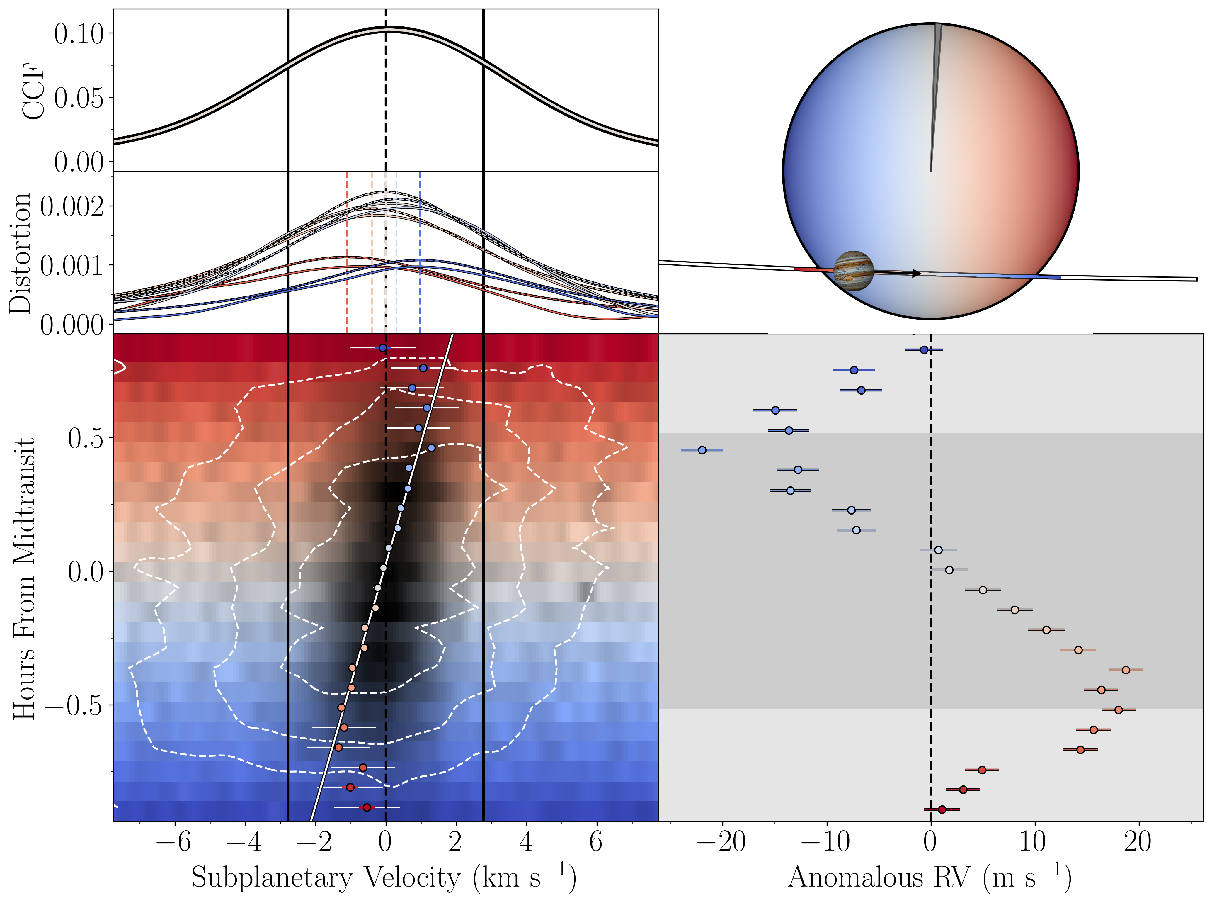
Figure 1: The Rossiter-McLaughlin effect displayed in four ways, for the illustrative case of WASP-50. Top right: Schematic of the planet transiting the stellar disk. The wedge represents the best-fit $\lambda$ and its uncertainty. The color scheme is based on the star’s rotational Doppler shift; the same color scheme is used in the top left and lower left panels to convey the location of the planet on the star. Top left: Spectral lines. The thick black curve is the average out-of-transit cross-correlation function (CCF) and the superimposed white curve is a CCF observed near mid-transit. Middle left: Spectral line distortions. Shown are the results of subtracting five of the in-transit CCFs from the mean out-of-transit CCF. Solid curves show the data. Dashed curves are the best-fit Lorentzian profiles, with vertical lines marking their centers. The color coding is done according to the apparent velocity anomaly going from redshifted (in red) to blueshifted (in blue). Bottom left: The Doppler shadow. Each row shows the spectral line distortion at a particular time. The white contours are amplitude levels of the distortion. Each small circle marks the best-fit subplanetary velocity (the Doppler shift of the portion of the star directly behind the planet’s center), with colors that convey the corresponding anomalous radial velocity shown in the lower right panel. Dark vertical lines mark the measured $v\sin i_{\star}$, and the diagonal white line is the best-fit trajectory. Bottom right: Anomalous radial velocities. The dark shaded area is the range of times when the planet’s silhouette is completely contained within the stellar disk.

3.3 The Rossiter-McLaughlin effect

The RM effect is the distortion of a star’s absorption lines that arises from the combination of stellar rotation and a transiting planet. During a transit, the planet prevents the light from a portion of the photosphere from contributing to the disk-integrated spectral line. The missing spectral component causes the velocity profile of the spectral lines to have a slightly reduced flux at velocities centered on the rotational Doppler shift of the star at the “subplanetary” point, i.e., the point on the the star directly behind the center of the planet. Observations of the RM effect can therefore be used to determine the time series of subplanetary velocities, or equivalently, the trajectory of the transiting planet relative to the stellar rotation axis.

Neglecting differential rotation, the RM effect is mainly a function of $\lambda$, $v\sin i_{\star}$, $R_{\rm p}/R_{\star}$, and the transit impact parameter $b\equiv d/R_{\star}\cos i$, where $d$ is the star-planet distance at the time of conjunction. For precise modeling it is also necessary to take into account limb darkening and non-rotational spectral line broadening. To model non-rotational broadening due to the star, we used the Gray (2005) model with parameters for the velocity spread generated by microturbulence ($\xi_{\star}$) and macroturbulence ($\zeta_{\star}$). We included a separate term for instrumental broadening, another source of non-rotational broadening. We neglected the effects of differential rotation and the convective blueshift, which for solar-type stars are not expected to produce detectable effects given the quality of our data (and indeed our modeling did not uncover any evidence for those effects, with one possible exception; see Section 4.12.1). We did not model the effects of starspots, flares, or pulsations, since there was no evidence for such phenomena in our data.

The RM effect has been analyzed as a distortion of individual spectral lines (e.g., Albrecht et al., 2007), as distortion of the spectral cross-correlation function (e.g., Cegla et al., 2016a), or as an “anomalous RV” obtained by an ordinary radial-velocity extraction code to a spectrum affected by the RM effect (e.g., Queloz et al., 2000). We used a combination of these approaches, depending on the system, as described below.

We fitted the spectral CCFs with a parameterized model that incorporates the RM effect, using a code first described by Knudstrup & Albrecht (2022) and Knudstrup et al. (2023a). In this model, the stellar disk is discretized (with a radius of 100 pixels) and a spectrum is assigned to each pixel according to the model parameters for limb darkening, stellar rotation, and non-rotational broadening. A disk-integrated spectral line is created by summing the spectra of all pixels that are not concealed by the planet, and the disk-integrated line profile is compared to the observed spectral CCF.

An alternative is to fit the time series of subplanetary velocities derived from the residuals between the out-of-transit CCF and the in-transit CCFs. The subplanetary velocity is calculated as

$$v_{p}(t)=v\sin i_{\star}x(t)\,,$$ (1)

where $x(t)$ is the distance from the projected rotation axis divided by the stellar radius. Once the orbital parameters are chosen, $x(t)$ can be calculated. It is also instructive to calculate $x$ at the times of ingress ($x_{1}$) and egress ($x_{2}$) (Albrecht et al., 2011):

$$\begin{split}x_{1}&=\sqrt{1-b^{2}}\cos\lambda-b\sin\lambda\,,\\ x_{2}&=\sqrt{1-b^{2}}\cos\lambda+b\sin\lambda\,.\end{split}$$ (2)

Therefore, the very nearly linear trajectory of the planet can be calculated as a function of time for given values of $t$, $T_{\rm c}$, the transit duration, $b$, and $\lambda$.

The simplest and most common approach is to fit a time series of anomalous RVs. In the model, the anomalous RV is computed as a function of $v_{p}$ by taking into account the size of the planet’s shadow, the limb darkening function, and the response of the radial-velocity extraction code to the RM distortion; for this purpose we used the code described by Hirano et al. (2011).

The different ways to sense the RM effect are illustrated in Fig. 1 for the case of WASP-50. For all 19 systems in our sample, we fitted the time series of anomalous RVs (the “RV-RM” method). For some systems, we also analyzed the distortions of the CCF, or fitted the time series of subplanetary velocities. Multiple methods were used to test for consistency in the results, and because for some systems it seemed plausible that the more sophisticated models would give more information about $\lambda$. In general, we expect line-profile modeling to be advantageous when $(R_{\rm p}/R_{\star})^{2}v\sin i_{\star}$ is larger than the non-rotational broadening (Albrecht et al., 2022).

We determined the best-fit parameters and their uncertainties via Markov Chain Monte Carlo (MCMC) sampling of the posterior probability distribution in parameter space. We used the emcee package (Foreman-Mackey et al., 2013). To ensure convergence we both inspected the chains visually and calculated the rank normalized R-hat. As mentioned above, we always fitted the the transit light curve alongside the spectroscopic data.

When fitting the RVs and the line distortion directly, we used Gaussian priors for the macroturbulence and microturbulence parameters, and we adopted a fixed value for the instrumental broadening parameter of each spectrograph (see Table 2). The mean values for our Gaussian priors were obtained from the relationships presented by Doyle et al. (2014) for stars with $T_{\mathrm{eff}}\in\mathclose{[}5200\leavevmode\nobreak\ \mathrm{K},6400\leavevmode\nobreak\ \mathrm{K}\mathclose{]}$ and $\log g\in\mathclose{[}4.0,4.6\mathclose{]}$, and Bruntt et al. (2010) for stars with $T_{\mathrm{eff}}\in\mathclose{[}5000\leavevmode\nobreak\ \mathrm{K},6500\leavevmode\nobreak\ \mathrm{K}\mathclose{]}$ and $\log g>4.0$. The width of the prior in all cases was 1 km s^-1.

We note that the properties of WASP-136, TOI-813, and HD 118203 are on the borderline of the range of properties for which the aforementioned relationships involving turbulent broadening are applicable; we applied them anyways. On the other hand, the properties of WASP-172 and LTT 1445A are far outside the applicable ranges. For WASP-172 ($T_{\mathrm{eff}}=6900\pm 150$ K), we expect a high macroturbulent velocity. We chose $6.0$ km s^-1 and increased the width of the prior to $4.0$ km s^-1 to reflect our uncertainty. For the microturbulent velocity, we adopted $\xi_{\star}=1.5\pm 1.5$ km s^-1. In the other end of the spectrum, we expect the turbulent velocities of the M dwarf LTT 1445A to be smaller. We chose $\zeta=1.0\pm 1.0$ km s^-1 and $\xi_{\star}=1.0\pm 1.0$ km s^-1. All of the priors are summarized in Table 5.

For each system, we performed two RV-RM analyses, one in which we adopted a uniform prior on $v\sin i_{\star}$, and one in which we applied a Gaussian prior on $v\sin i_{\star}$ based on the observed line broadening of the out-of-transit spectrum (Table 6) and a width of $0.5$ km s^-1. When analyzing the line profiles or Doppler shadow, we always applied the Gaussian prior on $v\sin i_{\star}$.

When fitting the time series of subplanetary velocities, we did not simultaneously fit the light curve. Instead, we applied Gaussian priors on $P$, $T_{0}$, $R_{\rm p}/R_{\star}$, $i$, and $a/R_{\star}$ based on an external fit to the light curve, and adopted uniform priors on $\lambda$ and $v\sin i_{\star}$.

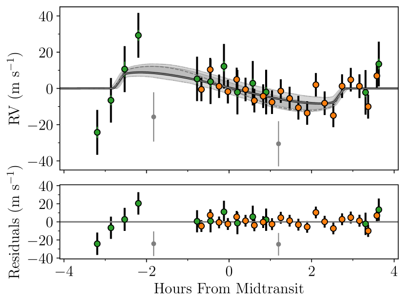
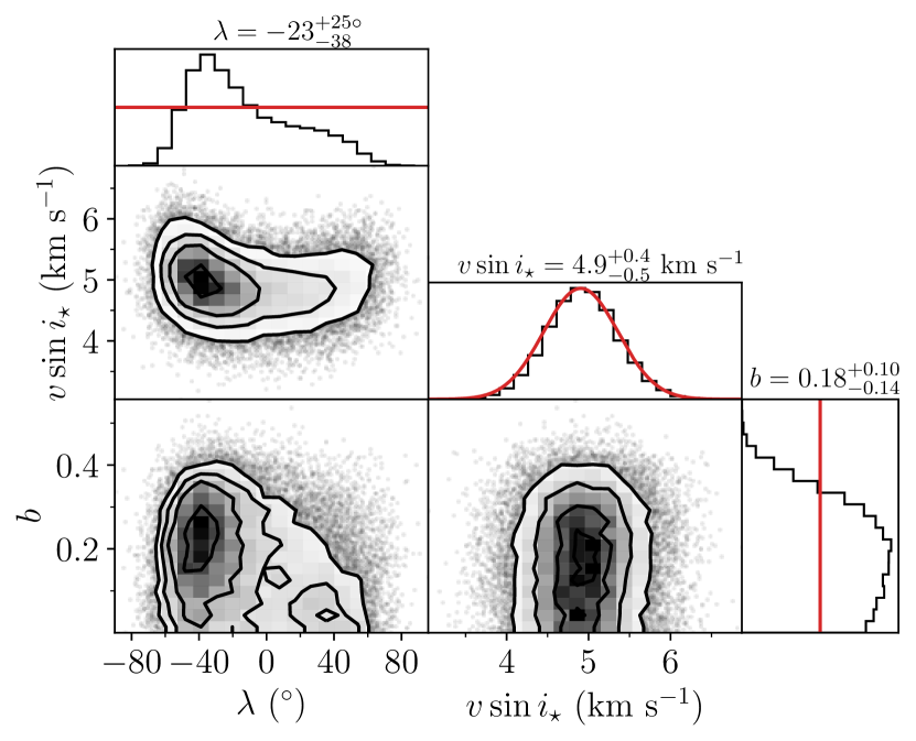
Figure 2: The RM effect observed in HD 118203. Left: Time series and residuals of the FIES+ RVs (orange) and FIES RVs (green). The black curve is the best-fit model and the gray shading shows the 1 and 2$\sigma$ confidence intervals created by randomly drawing values from the MCMC chains for $b$, $v\sin i_{\star}$, $R_{\rm p}/R_{\star}$, and $\lambda$. The dashed curve is the best-fit model assuming $\lambda=0^{\circ}$. Gray circles are the data that were obtained during poor atmospheric conditions and were excluded from the analysis. Right: Correlations between $\lambda$, $v\sin i_{\star}$, and $b$. The red lines illustrate the prior that was applied (either uniform or Gaussian).

In some cases, to boost the SNR, we stacked the CCFs from different exposures in a way similar to Johnson et al. (2014), but with a code based more directly on the work of Hjorth et al. (2019). In these cases, we extracted the Doppler shadow as shown in Fig. 1, and then transformed the velocities by correcting for the slope in Eq. (2). The white line/slope in Fig. 1 is in this way used to bring each pixel directly beneath it in the Doppler shadow to be located at $0$ km s^-1. We then collapse the slope corrected shadow by summing along the ordinate (time stamps) for a given geometry ($\lambda$,$v\sin i_{\star}$,$b$). When the model parameters match reality, we expect to see a sharp peak at $0$ km s^-1 in the summed spectrum, and we found the height of the peak by fitting a Gaussian to it. Hjorth et al. (2019) did this for a dense grid in the parameter space of $b$, $v\sin i_{\star}$, and $\lambda$. For our purposes, since $b$ was always tightly constrained by the light curve, we neglected the uncertainty in $b$ and simply adopted the best-fit value from the RV-RM method. We then searched the 2-d parameter space of $v\sin i_{\star}$ and $\lambda$ for the strongest peak; in practice this was done by fitting a 2-d Gaussian function. We did not run an MCMC when stacking the CCFs, nor did we fit the light curve simultaneously. The quoted uncertainties are taken as the widths ($\sigma$s) of the fitted 2D Gaussian and as such do not reflect the actual precision. The resulting values therefore only serves as an indication to whether the results in ($\lambda$,$v\sin i_{\star}$) from the RV-RM runs are in (qualitative) agreement with that seen in the CCFs.

4 Analysis of the individual systems

Below, we describe the particulars of each system, our analysis, and the results. The details for each system are also summarized in Table 1, Table 4, and Table 3.

4.1 HD 118203

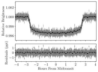
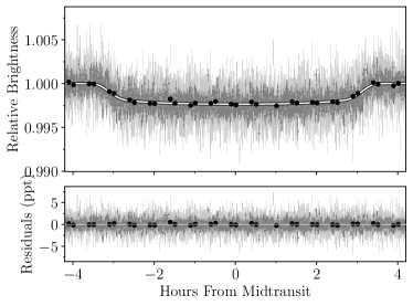
(a) HD 118203 b	(b) HD 149193 b
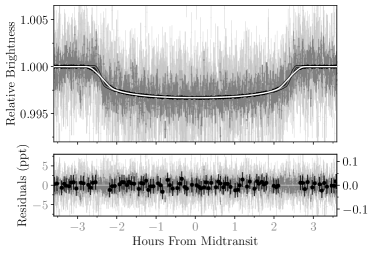
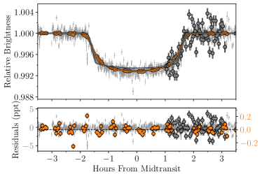
(c) K2-261 b	K2-287 b (d)
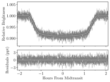
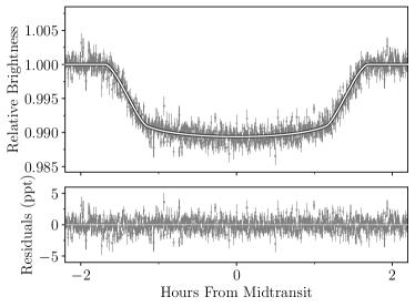
(e) KELT-3 b	(f) KELT-4Ab

Figure 39: Phasefolded light curves. The best-fitting models are shown as the white line in the top panel and the residuals are given in the bottom panel. (a) HD 118203 b: TESS 2 min. cadence data shown as gray points with error bars. Black markers are binned data in $\sim$10 min. intervals. (b) HD 149193 b: TESS light curves 20 sec., 2 min., and 30 min. cadence data are shown in light gray, gray, and black, respectively. (c) K2-261 b: K2 light curve in black, TESS 20 sec. and 2 min. in light gray and gray, respectively. A light curve for each passband is shown. (d) K2-287 b: K2 30 min cadence shown in orange with CHEOPS 1 min. and ground-based 2 min. observations in light gray and gray, respectively. A light curve for each passband is also shown with a matching color. (e) KELT-3 b: TESS 2 min. cadence data shown in gray. (f) KELT-4Ab: TESS 2 min. cadence data shown in gray.

HD 118203 b was discovered by da Silva et al. (2006) through RV monitoring, and was later found to be a transiting planet by Pepper et al. (2020) using TESS data. TESS data are available for HD 118203 from Sectors 15, 16, 22, and 49 with a 2-minute cadence. The planet is a hot Jupiter on an eccentric orbit around a slightly evolved G-type star (Pepper et al., 2020). The TESS data centered on the mid-transit time are shown in Fig. 39.

We observed two transits of HD 118203 b with FIES. The first transit began on March 24, 2020 at around UT 21:00 and ended at 04:15. The observations were interrupted twice due to high humidity. The exposure time was 900 s and the time between exposures was 1171 s, with the time in between spent on ThAr calibration. Two exposures on this night were heavily affected by weather and the resulting RVs deviate significantly from the rest (see the gray points in Fig. 2). These two data points were omitted from the analysis.

Since the first transit had been interrupted by the weather, we organized observations of a second transit on the night starting on June 18, 2022. Unfortunately, the first part of the transit was missed because the telescope was being used to observe a target-of-opportunity. Our transit observations started at around UT 22:30 and continued until around 03:00. As the FIES spectrograph was refurbished in the summer of 2021 resulting in an improved throughput, we opted for a shorter exposure time of 600 s for the second transit, which resulted in a sampling time of around 768 s. We note that the refurbishment introduced an offset in RV between observations. As such we allowed the systemic velocity parameter to differ between the two nights: $\gamma_{\rm FIES}$ applies to the observations taken before summer 2021, and $\gamma_{\rm FIES+}$ applies to subsequent observations.

As mentioned above (Section 3) we performed two MCMC analyses, one with a uniform prior on $v\sin i_{\star}$ and one with a Gaussian prior. For this system, the results differed substantially. The uniform prior in $v\sin i_{\star}$ yielded $\lambda=$ $-74^{+6}_{-9}$^∘ and the Gaussian prior yielded $-23^{+25}_{-38}$^∘. The data obtained from the first transit observations are obviously very noisy. This paired with the second transit observations only covering the second half of the transit meant that the amplitude of the signal was allowed to vary significantly, which made $v\sin i_{\star}$ wander off to large values when applying applying a uniform prior. In this case $v\sin i_{\star}$ ended up being $26^{+13}_{-23}$ km s^-1, which is both poorly constrained and at face value in disagreement with the value we derived and the value found in the literature. Therefore, our best estimate is $-23^{+25}_{-38}$^∘ based on the analysis in which $v\sin i_{\star}$ was subjected to a Gaussian prior.

4.2 HD 148193

HD 148193 is also known as TOI-1836. The planet HD 148193 b (TOI-1836.01) was confirmed and characterized by Chontos et al. (2024). It is a warm Saturn around a subgiant star in a system with a companion star. A second transiting planet candidate was announced later (TOI-1836.02), which is potentially a super-Earth-sized planet on a 1.7-day orbit. However, the signal-to-noise ratio of the observed transits is modest and the planet remains unconfirmed.

TESS data are available with 30-min cadence from Sectors 16 and 25; with 2-min cadence in Sectors 23, 24, 49, 50, 51, and 52; and with 20-sec cadence in Sector 56. The light curve is shown in Fig. 39.

We used HARPS-N at the TNG to observe a transit of HD 148193 b. We started observations around UT 21:30 and continued until UT 05:45 on the night starting on June 15, 2021. The exposure time was 1140 s. After accounting for overheads, the sampling time was 1168 s. The transit observations are shown in Fig. 3.

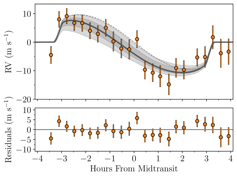
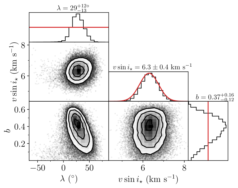
Figure 3: The RV-RM effect for HD 148193. Same as for Fig. 2, but with RVs from HARPS-N.

The combined fit to the light curve and RVs gave $\lambda=$$29^{+12}_{-13}$^∘. However, we obtained only one pre-ingress RV and two post-egress RVs. With such sparse out-of-transit data, any mismatch between the out-of-transit RV slope observed on that night and the calculated slope based on the planet’s orbital parameters can lead to systematic errors. This problem, combined with the reasons discussed in Section 3.3 and the large projected rotation speed of this system ($\sim 6$ km s^-1), led us to analyze the line distortions and Doppler shadow. We found $\lambda=$ $14^{+7}_{-8}$^∘, with results shown in Fig. 4. We adopted the value from the Doppler-shadow analysis as our best estimate for $\lambda$.

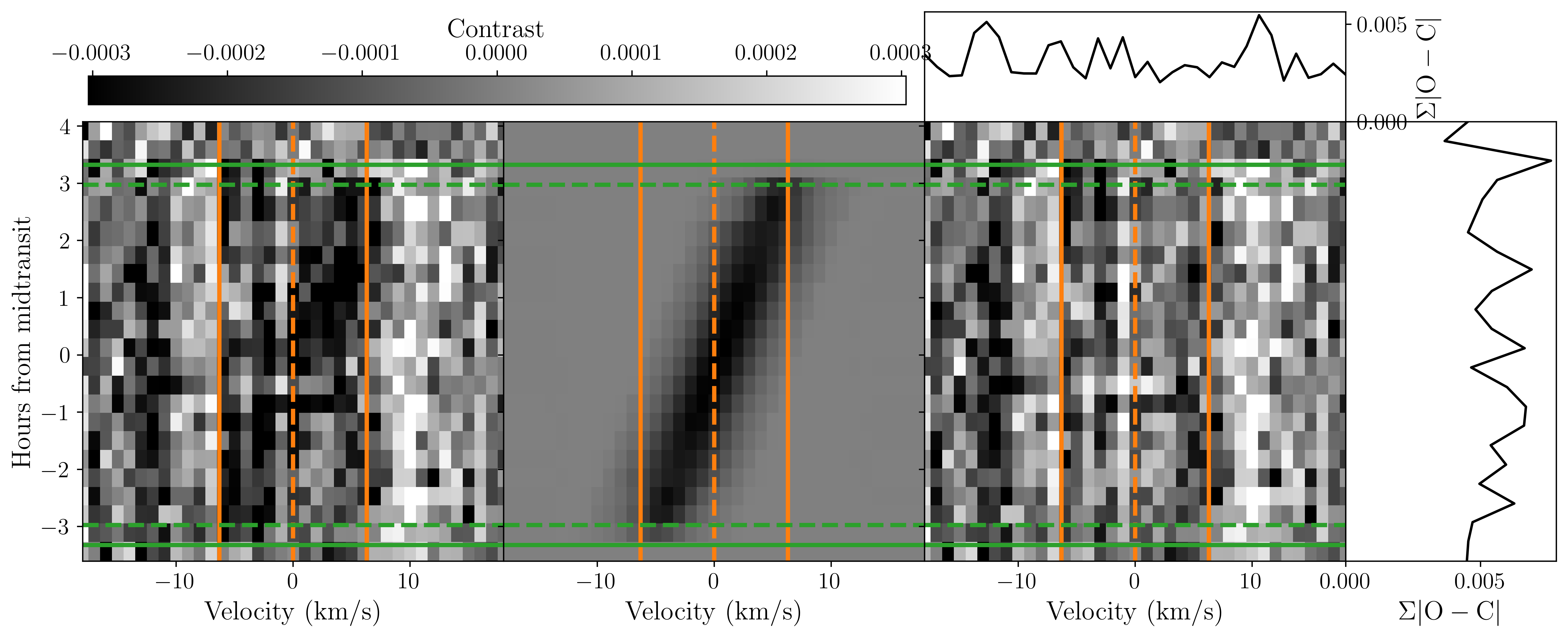
Figure 4: Doppler shadow for HD 148193. Left: The observed Doppler shadow created by subtracting the in-transit CCFs from an average out-of-transit CCF. Middle: Model Doppler shadow. Right: Residuals from subtracting the model from the observed shadow. The summed residuals are given in the adjacent panels. The color bar demarcate the contrast. Green horizontal lines denote points of first (solid), second (dashed), third (dashed), and fourth (solid) contact. The solid, orange, vertical lines denote $\pm$$v\sin i_{\star}$.

4.3 K2-261

K2-261 was observed in Campaign 14 of the K2 mission with 30-minute cadence. The planet was confirmed and characterized independently by Johnson et al. (2018), who named the planet K2-261 b, and Brahm et al. (2019), who named it K2-161 b. Here, we adopt the name K2-261 b, which is also the name chosen by Ikwut-Ukwa et al. (2020). The planet is a warm Saturn-sized planet on an eccentric orbit around a slightly evolved G-type star (Brahm et al., 2019). K2-261 was observed by TESS in Sectors 9, 35, 45, and 46. TESS data are available with 2-min cadence in Sectors 9, 45, and 46, and with 20-sec cadence in Sector 35. The light curve is shown in Fig. 39.

For K2-261 b we used HARPS-N at the TNG to observe a transit. The data are shown in Fig. 5. We carried out the observations on the night starting on March 24, 2022, from around UT 20:15 until 03:30. We used an exposure time of 600 s, resulting in a sampling time of around 625 s.

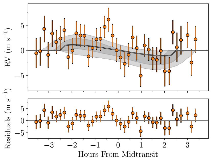
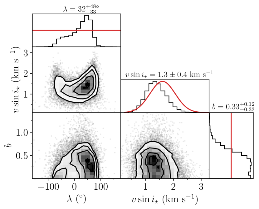
Figure 5: The RV-RM effect for K2-261. Same as for Fig. 2, but with RVs from HARPS-N.

We found a value for $v\sin i_{\star}$ for K2-261 that is somewhat smaller than the value of $3.70\pm 0.17$ km s^-1 reported by Johnson et al. (2018), both from our BF analysis ($1.6$ km s^-1) and from our RM observations. The amplitude of the signal is not as strong as would be expected if $v\sin i_{\star}$ were really $3.70\pm 0.17$ km s^-1. A uniform prior on $v\sin i_{\star}$ resulted in $v\sin i_{\star}$ $=1.0^{+0.5}_{-0.6}$ km s^-1 and $\lambda=$ $29^{+35}_{-56}$^∘, and applying a Gaussian prior yielded a value for the projected obliquity of $32^{+48}_{-33}$^∘. We adopt the latter as our best estimate for $\lambda$.

4.4 K2-287

K2-287 was observed in Campaign 15 of the K2 mission. Jordán et al. (2019) discovered and characterized the system, finding the host to be a G-dwarf and the planet to be a warm Saturn-sized planet on an eccentric orbit.

We observed a transit of K2-287 b using ESPRESSO. Observations were carried out from UT 02:06 to 06:16 on the night July 6, 2021. The exposure time was 540 s, which including overhead comes out to a sampling time of roughly 600 s. The RVs derived from the spectra are shown in the left half of in Fig. 6.

Given the 30-min time averaging of the K2 photometric time series, and the rather long orbital period of the planet, the K2 light curve is relatively poorly sampled. Furthermore, this star has evaded TESS observations to this point. As of the time of writing, there are no scheduled TESS observations that would cover this star.

This situation, along with the lack of post-egress spectroscopoic observations, prompted us to search for a suitable archival ground-based light curve covering the egress. The one we found was obtained at the Adams Observatory at Austin College on the night starting June 30th, 2018. More recently, the system was observed with the CHaracterising ExOPlanet Satellite (CHEOPS; Benz et al., 2021). Borsato et al. (2021) observed three separate transits with a 1-min cadence, and the data from all three provide good coverage of the entiure transit. In our analysis, we included the de-trended light curves presented by Borsato et al. (2021). The K2, CHEOPS, and ground-based light curves are shown in Fig. 39.

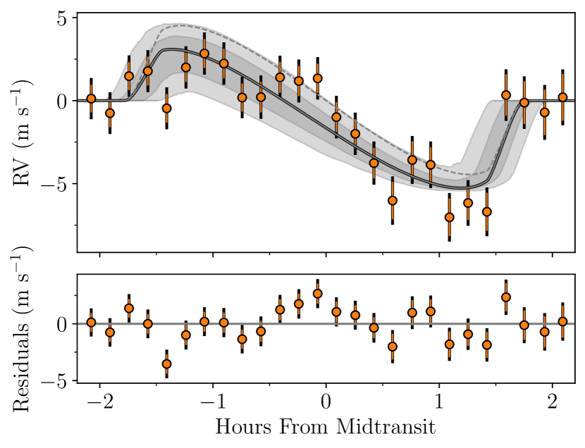
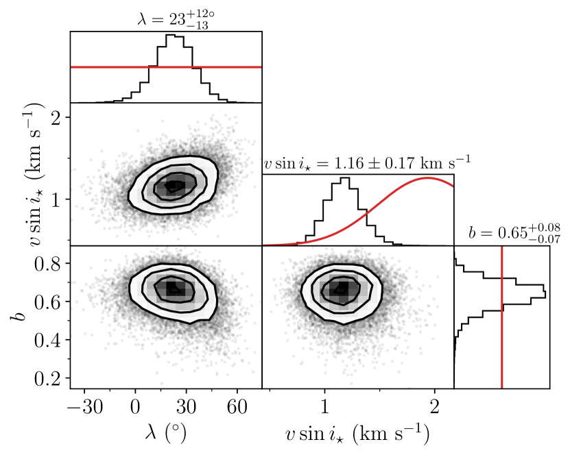
Figure 6: The RV-RM effect for K2-287. Same as for Fig. 2, but with RVs from ESPRESSO.

The two RV-RM analyses yielded similar results for $\lambda$, with $21^{+14}_{-11}$^∘ for the case of a uniform prior on $v\sin i_{\star}$ and $23^{+12}_{-13}$^∘ for the case of a Gaussian prior on $v\sin i_{\star}$. We also investigated the in-transit subplanetary velocities, which are shown in Fig. 7 along with the best-fitting slope. In addition to the errors obtained when extracting the location of the subplanetary velocities, we add two different jitter terms in quadrature; one for the epochs taken when the planet is completely within the stellar disk (dark gray area in Fig. 7), and another when the planet is at the limb (light gray). This is because there generally (see, e.g, WASP-50 in Section 4.12) seems to be some additional scatter in the subplanetary velocities at the limb, which the errors from fitting a Gaussian to the residual peak do not fully capture.

From this we found values of $v\sin i_{\star}$ $=1.16\pm 0.19$ km s^-1 and $\lambda=$ $37^{+8}_{-9}$^∘, which are consistent with the values derived from the RV-RM effect. Somewhat arbitrarily, we adopt $\lambda=$ $23^{+12}_{-13}$^∘ as our best estimate; this derives from the RV-RM fit with a Gaussian prior on $v\sin i_{\star}$. The posterior distributions are shown in Fig. 6.

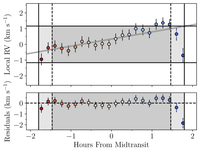
Figure 7: Subplanetary velocities for K2-287. Subplanetary velocities for K2-287 with color-coding as described in Fig. 1. The dark shaded area corresponds to the time the planet is completely within the stellar disk and the light shaded area denote ingress and egress. The errorbars include a jitter term, where two separate terms have been added in quadrature; one for the epochs for the full transit and one for the epochs when the planet is partially outside of the limb of the star. The horizontal black lines in the top panel mark $v\sin i_{\star}$ from the fit.

4.5 KELT-3

Pepper et al. (2013) reported the discovery of the KELT-3 system, which consists of a hot Jupiter orbiting a late F star. TESS data with 2-min cadence are available from Sectors 21 and 48. The light curve is shown in Fig. 39.

We used FIES to observe a transit on the night starting April 8, 2022, with observations starting around UT 20:50 and continuing until UT 01:30 April 9, 2022. The exposure time was 900 s, which including overhead resulted in a cadence of 1080 s. The RM-RV effect is shown on the left side of Fig. 8.

As was the case for K2-261, the value for KELT-3’s projected rotation velocity drawn from the literature ($10.2\pm 0.5$ km s^-1; Pepper et al., 2013) is higher than what we obtained from the BF method ($7.6$ km s^-1). The observed amplitude of the RM effect suggests that the true $v\sin i_{\star}$ is even lower. Our RV-RM analysis gave $6.4\pm 0.4$ km s^-1 when using a uniform prior in $v\sin i_{\star}$, and $\lambda$ = $-5\pm 4$^∘. When we applied a Gaussian prior on $v\sin i_{\star}$, we obtained $-6\pm 5$^∘.

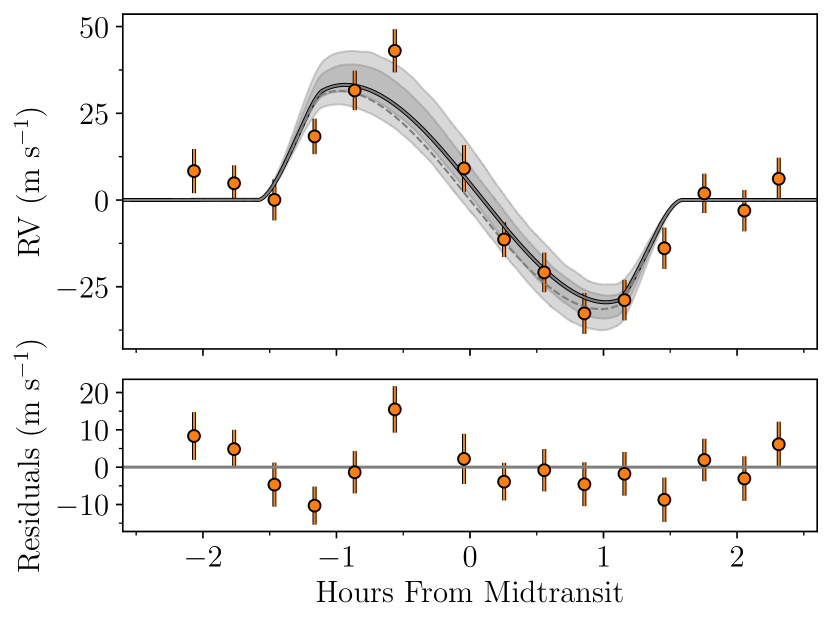
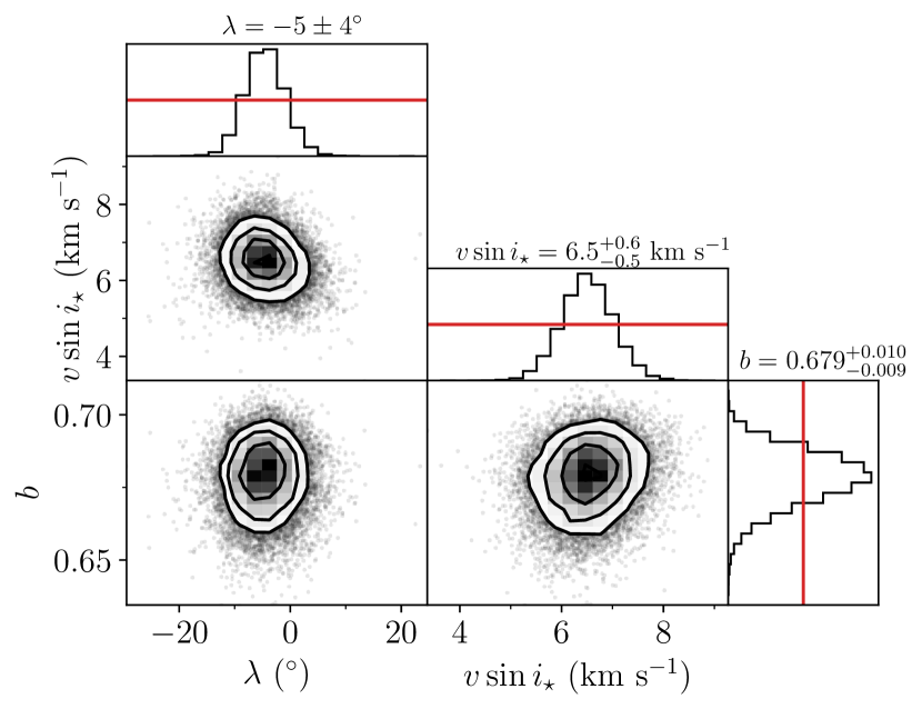
Figure 8: KELT-3. Same as for Fig. 2. Here also with RVs from FIES.

Given the discrepancy between the different measurements of $v\sin i_{\star}$, we decided to look at the stacked CCFs resulting from our FIES spectra. In Fig. 9 we show the contours of the peak values obtained from stacking the CCFS on the 2D grid in the space of $v\sin i_{\star}$ and $\lambda$, compared to our posterior from the RV-RM fit. From this analysis we found $v\sin i_{\star}$ $=5.96\pm 0.03$ km s^-1 and $\lambda=1.06\pm 0.16^{\circ}$, implying that the system is well-aligned, and that $v\sin i_{\star}$ is closer to 6 km s^-1 than the value of $10.2\pm 0.5$ km s^-1 reported by Pepper et al. (2013). Although evidently the uncertainties in some or all of the $v\sin i_{\star}$ determinations have been underestimated, we believe that the stacked-CCF method gives the most reliable result for $v\sin i_{\star}$.

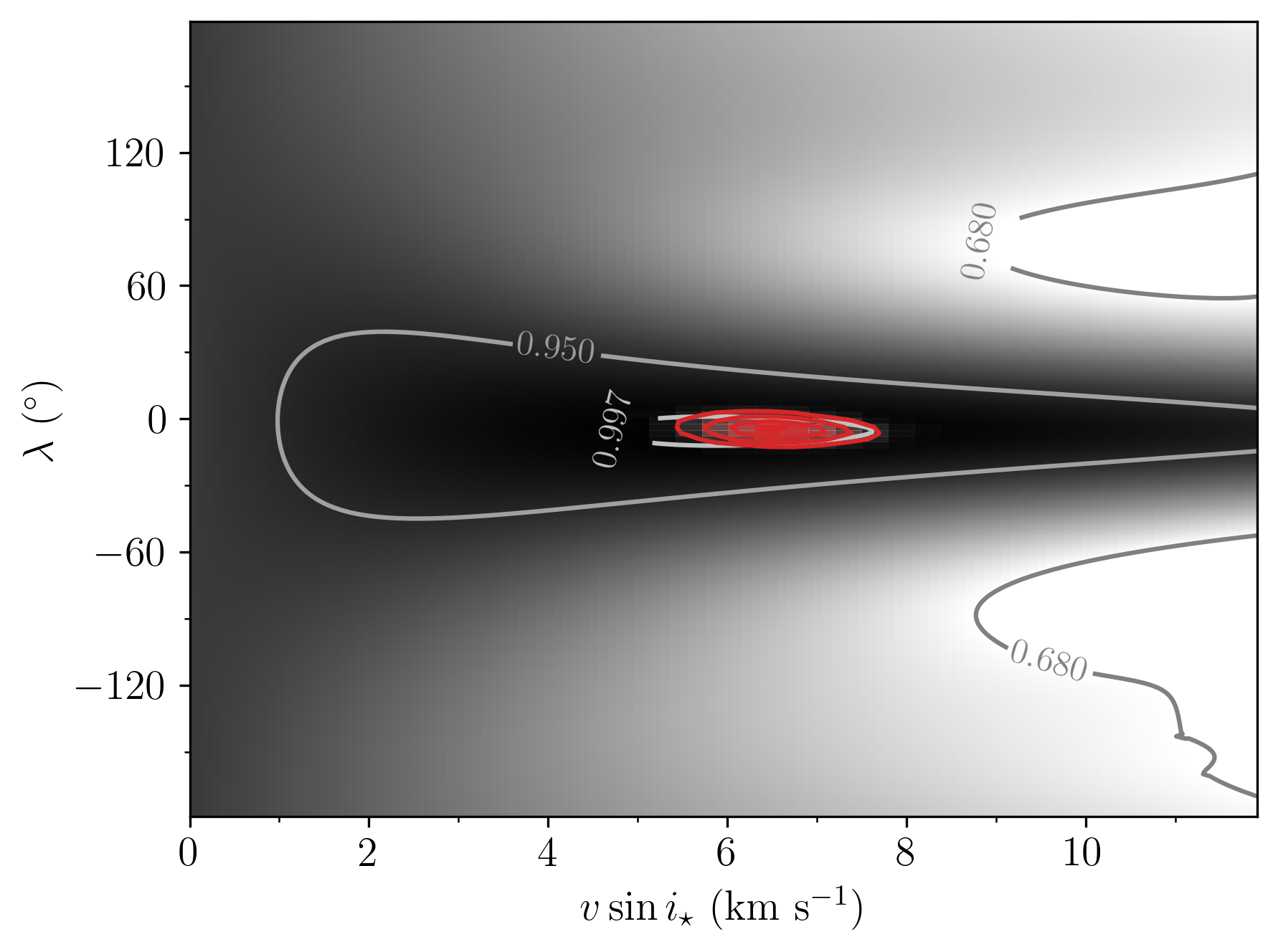
Figure 9: Peak of the stacked CCFs of KELT-3. The peak of the stacked CCFs of KELT-3 created by assuming the best-fitting value of $b$ from the RV-RM fit. The gray contours show a peak around ($v\sin i_{\star}$,$\lambda$)=($6.0\leavevmode\nobreak\ \mathrm{km}\leavevmode\nobreak\ \mathrm{s}^{-1}$,$1.0^{\circ}$). The red contours are the same as created from the posterior shown to the right in Fig. 8.

This lends further credence to the RV-RM fit with a uniform prior on $v\sin i_{\star}$, and as our observations of KELT-3 have a high SNR and cover the transit very well. We therefore adopt the result from this RV-RM fit, $\lambda=$ $-5\pm 4$^∘, as our best estimate for this system.

4.6 KELT-4A

KELT-4 is a hierarchical triple star system discovered by Eastman et al. (2016). The primary star, KELT-4A, is an F star orbited by a hot Jupiter. The close binary system KELT-4BC is engaged in a wide orbit with KELT-4A. TESS data are available from Sector 48 with 2-min cadence. The light curve is shown in Fig. 39. Since the TESS cameras cannot resolve KELT-4A from KELT-4BC, we included a dilution factor in our analysis of $\delta M=3.5\pm 0.1$ (estimated from Table 3 in Eastman et al., 2016) to correct for the light from KELT-4BC.

On the night starting January 27, 2021, we observed a transit of KELT-4Ab, starting the observations UT 01:40 and ending them UT 06:45 January 28, 2021. The exposure time was 900 s, meaning the effective sampling was a spectrum every 1090 s.

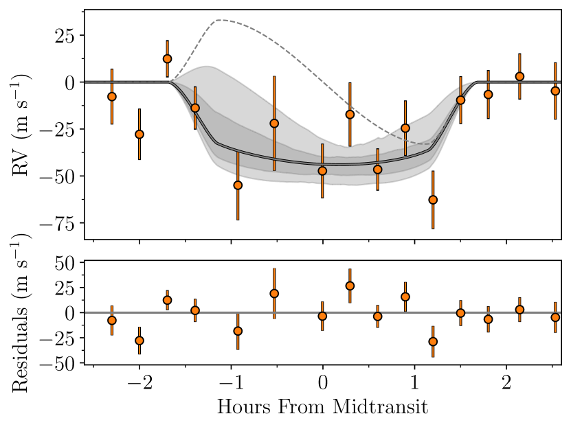
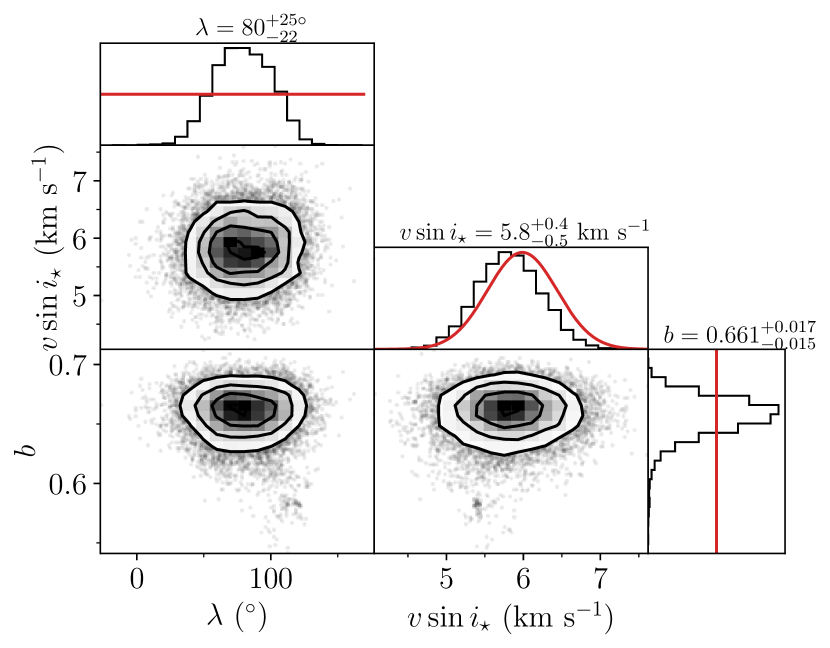
Figure 10: KELT-4A. Same as for Fig. 2. Here also with RVs from FIES.

The observations are shown in Fig. 10 with our results from a run invoking a Gaussian prior on $v\sin i_{\star}$. From this we got $\lambda=$ $80_{-22}^{+25}$^∘. Applying a uniform prior on $v\sin i_{\star}$ we found $\lambda=$ $77_{-23}^{+25}$^∘. Evidently, applying a Gaussian or a uniform prior on $v\sin i_{\star}$ makes little difference, despite the somewhat noisy data, most likely because of the rather large impact parameter and large misalignment.

As for KELT-3, we investigated the stacked CCFs for this system. The results coincided with the result from our RV-RM fit, and when fitting a 2D Gaussian to the grid of $v\sin i_{\star}$ and $\lambda$ we obtained values of $v\sin i_{\star}$ $=6.0\pm 0.4$ km s^-1 and $\lambda=88.9\pm 0.5^{\circ}$. The results are consistent with the polar configuration implied by the RV-RM fit. Our best estimate for $\lambda$ for this system, $80_{-22}^{+25}$^∘, is based on the RV-RM fit with a Gaussian prior on $v\sin i_{\star}$.

4.7 LTT 1445A

LTT 1445 is a triple star system consisting of three M-dwarfs. The primary star hosts an Earth-sized planet on a 5-day orbit, LTT 1445Ab, which was discovered by Winters et al. (2019). A second transiting planet, LTT 1445Ac, was reported by Winters et al. (2022), and an RV signal from a third planet was detected by Lavie et al. (2023). The orbit of LTT 1445Ab is sandwiched between the orbits of the other two planets.

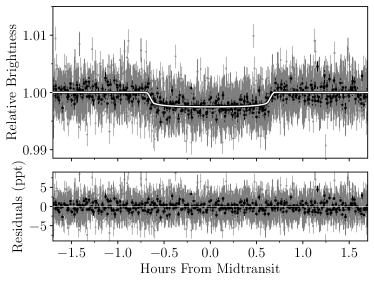
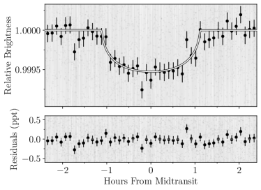
(a) LTT 1445Ab	(b) TOI-451Ab
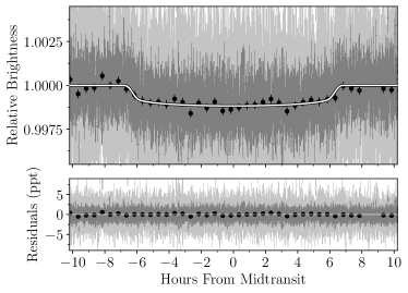
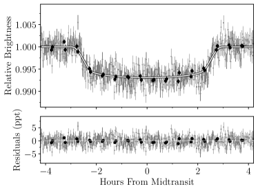
(c) TOI-813 b	(d) TOI-892 b
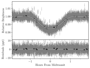
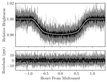
(e) TOI-1130 c	(f) WASP-50 b

Figure 40: Phasefolded light curves. Same as in Fig. 39. (a) LTT 1445Ab: Black TESS 2 min. and gray TESS 20 sec. (b) TOI-451Ab: Unbinned 2 min. cadence data are shown in gray and in black the binned ($\sim$6 min.) data are shown. (c) TOI-813 b: TESS 20 sec., 2 min., and 30 min. cadence data are shown in light gray, gray, and black, respectively. (d) TOI-892 b: TESS 2 min. and 30 min. cadence data are shown in gray and black, respectively. (e) TOI-1130 c: TESS 20 sec. and 30 min. cadence data shown in gray and black, respectively. (f) WASP-50 b: TESS 20 sec. and 2 min cadence data shown in gray and black, respectively.

LTT 1445A was observed by TESS in Sectors 4 and 31, and the data are available with 20-sec and 2-min cadence, respectively. The light curves show a photometric quasiperiodicity that probably arises from rotation of either star B or star C (Winters et al., 2019). To account for this rotational modulation, our model for the light curve including a GP with a kernel consisting of two stochastically driven damped harmonic oscillators. As the amplitude of the rotational modulation seemed to change between the two sectors (Winters et al., 2022), we did not require the hyperparameters to be the same in both sectors. The light curve is shown in Fig. 40.

We observed a spectroscopic transit of LTT 1445Ab employing HARPS-N. The observations were carried out on the night starting September 5th, 2020. We used an exposure time of 900 s, yielding a sampling time of 920 s. The first exposure was not useful because the telescope was erroneously aimed at LTT 1445BC. The remainder of the observations are shown in Fig. 11.

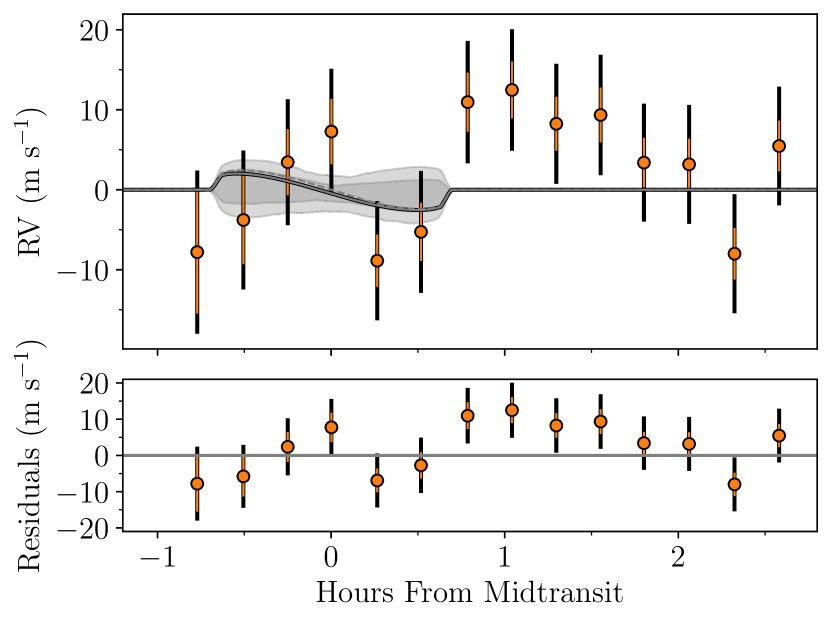
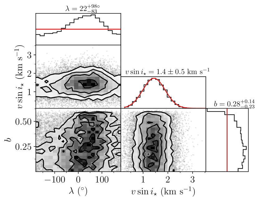
Figure 11: LTT 1445A. Same as for Fig. 2, but with RVs from HARPS-N.

As can be seen in Fig. 11 no RM effect is apparent in the RV data. Formally, we found $\lambda=$ $22_{-83}^{+98}$^∘, implying a gentle preference for a prograde orbit. However, as described by Albrecht et al. (2011), such low SNR results are probably even more uncertain than the formal uncertainty suggests.

Usually, if the RV-RM effect has a detectable amplitude, then the scatter of the RVs inside the transit should be larger than the scatter of the RVs outside the transit. For LTT 1445A, the in-transit scatter is $\sigma=5.9$ m s^-1 after subtracting the best-fit orbital solution. The out-of-transit scatter is $\sigma=7.1$ m s^-1 (dropping to $\sigma=6.0$ m s^-1 if the single pre-transit datum is excluded). The in-transit residuals relative to the best-fit RM model have a scatter of $\sigma=5.5$ m s^-1. In light of these results, we do not consider the RM effect to have been detected at all. Better results would probably require a bigger telescope.

4.8 TOI-451A

TOI-451 is a young multiplanet system in the Pisces–Eridanus stream consisting of the G-dwarf planet host, TOI-451A, and a wide-orbiting (likely) M-dwarf binary (Newton et al., 2021). The planetary system around TOI-451A consists of three planets with radii 1.9, 3.1, and 4.1 R_⊕ and periods of 1.9, 9.2, and 16 days. TESS observed the system in Sector 4, 5, and 31 with a cadence of 2 min. The TESS observations of TOI-451A are shown in Fig. 40.

We observed a transit of TOI-451Ab, the innermost and smallest planet, using ESPRESSO. The observations were carried out on the night starting on September 24, 2022, from around UT 04:15 until 08:30 September 25, 2022. The exposure time was set to 720 s, resulting in a spectrum every 755 s.

As reported by Newton et al. (2021), the light curve of TOI-451 displays a rather large amplitude rotational modulation. We therefore adopted the same kernel as for LTT 1445 (described in the previous section) instead of the Matérn-3/2 kernel. We included all three planets in our transit modeling. We applied Gaussian priors with values drawn from Newton et al. (2021) for the transit parameters to the two, outer planets (c and d) for which we did not observe a spectroscopic transit. For planet b we followed our usual approach.

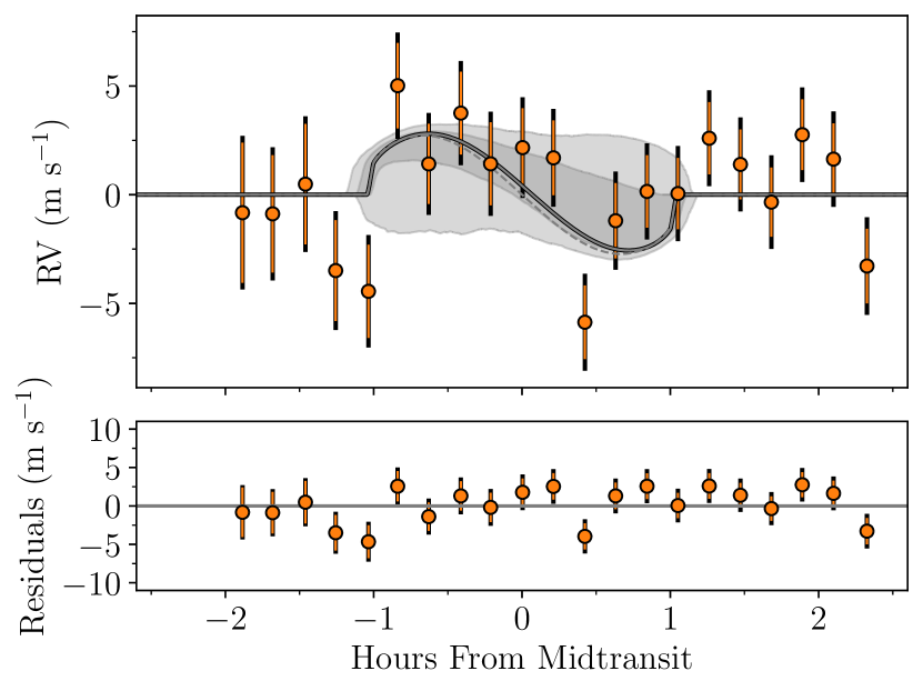
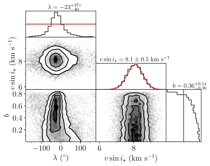
Figure 12: The RV-RM effect for TOI-451. Same as for Fig. 2, but with RVs from ESPRESSO.

The RV-RM analysis with a uniform prior on $v\sin i_{\star}$ gave $\lambda=$ $-27^{+64}_{-74}$^∘ and the analysis with a Gaussian prior gave $-23^{+37}_{-40}$^∘. All we can conclude is that the orbit is prograde.

We investigated the RV scatter in the same manner we did for LTT 1445. We obtained $\sigma=2.8$ m s^-1 and $\sigma=2.4$ m s^-1 for the in-transit and out-of-transit scatter, respectively, and when subtracting the RM effect from the in-transit data we found $\sigma=2.0$ m s^-1. With these results we cannot be confident that the RM effect was detected. For better results, one might observe a second transit of TOI-451Ab or give up and choose to observe one of the larger planets (for which opportunities to observe transits are rarer).

We did not use any results from LTT 1445A or TOI-451A in the ensemble analyses described in Section 5.2, Section 5.1, and Section 5.3. However, the results are displayed in Section 5.4, which focuses on multiplanet systems.

4.9 TOI-813

Eisner et al. (2020) used TESS data to discover a Saturn-sized planet on an 84-day orbit around this subgiant star. TESS data are available with 30-min cadence in Sector 2; 2-min cadence in Sectors 5, 8, 11, 30, 33, and 39; and 20-sec cadence in Sectors 27 and 61. Due to the planet’s long orbital period, transits only occurred during Sectors 2, 27, and 61. Fig. 40 shows the light curve.

We observed a transit of TOI-813 b on the night January 20, 2023, using ESPRESSO. The exposure time was set to 800 s, yielding a sampling time of around 832 s. This transit was simultaneously observed with TESS. We observed the transit starting just before ingress and continued for for 6.5 hours until the target set. These observations cover roughly half of the 13.14 hr transit as shown in Fig. 13.

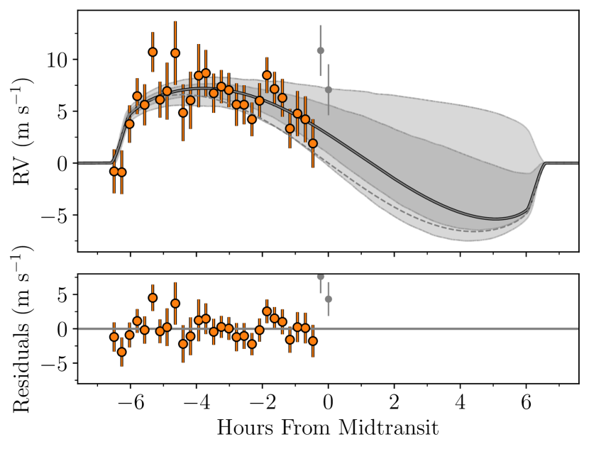
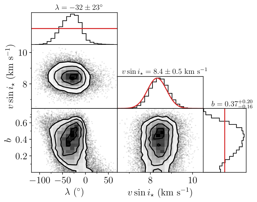
Figure 13: The RV-RM effect for TOI-813. Same as for Fig. 2, but with RVs from ESPRESSO.

In an attempt to cover as much of the transit as possible, the two last exposures were acquired through a large airmass ($>2.2$), and the RVs based on those exposures deviate from the trend established by the preceding RVs. Including the two high-airmass RVs in our fit resulted in $\lambda=-60^{+19}_{-21}$^∘ suggesting that the system is significantly misaligned. Omitting these two exposures yielded $-32\pm 23$^∘. In both cases described above, a Gaussian prior on $v\sin i_{\star}$ was applied. Excluding the last two exposures while running an MCMC with a uniform prior in $v\sin i_{\star}$, we obtained $-53^{+22}_{-25}$^∘ for $\lambda$.

We also analyzed the Doppler shadow for this system and found a value of $-53^{+25}_{-28}$^∘, which is more in-line with the results obtained using a uniform prior on $v\sin i_{\star}$ or including the two data points at high airmass. However, the lack of observations outside of the transit left us without a spectral CCF that is free of the RM effect.

Since only half of the transit was covered, we found it necessary to apply a Gaussian prior on $v\sin i_{\star}$ to obtain reliable results. We also decided not to trust the two high-airmass RVs. We adopt the resulting value of $-32\pm 23$^∘ as our best estimate of $\lambda$ for TOI-813. The RM effect has a high enough amplitude to be detectable using smaller telescopes and less precise spectrographs. Another observation covering the second half of the transit is warranted, and would allow us to be judge more definitively if the system is aligned or not.

4.10 TOI-892

TOI-892 b is a warm Jupiter on a circular orbit around an F-type dwarf (Brahm et al., 2020). The system was first observed by TESS in Sector 6 with 30 min cadence, and then in Sector 33 with 2-min cadence. Fig. 40 shows the light curve.

We used HARPS-N to observe a transit of TOI-892 b. We started observations around UT 19:15 and continued until 03:15 on the night starting on January 1, 2022. The exposure time was set to 960 s, which including overhead comes out to a sampling time of around 987 s. The observations were interrupted due to high humidity.

The results with and without the Gaussian prior on $v\sin i_{\star}$ are in agreement, giving $\lambda=$! $10^{+39}_{-35}$^∘ and $9^{+30}_{-23}$^∘, respectively. Since about half of the transit was not observed, the run including a Gaussian prior on $v\sin i_{\star}$ yielded a better constraint on $\lambda$, as one would expect.

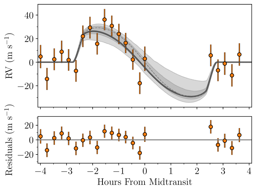
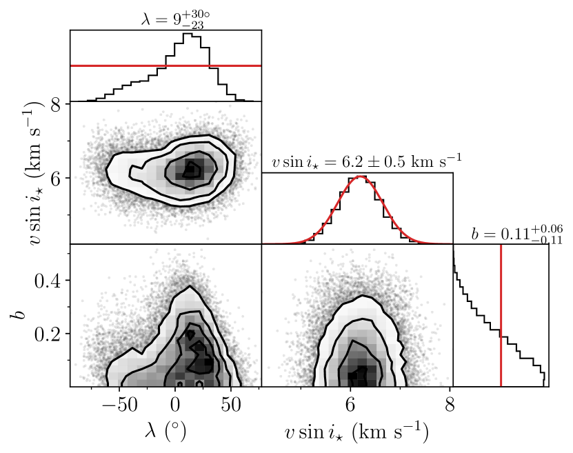
Figure 14: The RV-RM effect for TOI-892. Same as for Fig. 2, but with RVs from HARPS-N.

We analyzed the Doppler shadow and found $\lambda=$ $-12^{+18}_{-16}$^∘, which differs from the RV-RM results more than one would expect for two analyses of the same data. Since the the shadow shown in Fig. 15 looks convincing, we decided to adopt the value of $-12^{+18}_{-16}$^∘ as our best estimate of $\lambda$ for this system.

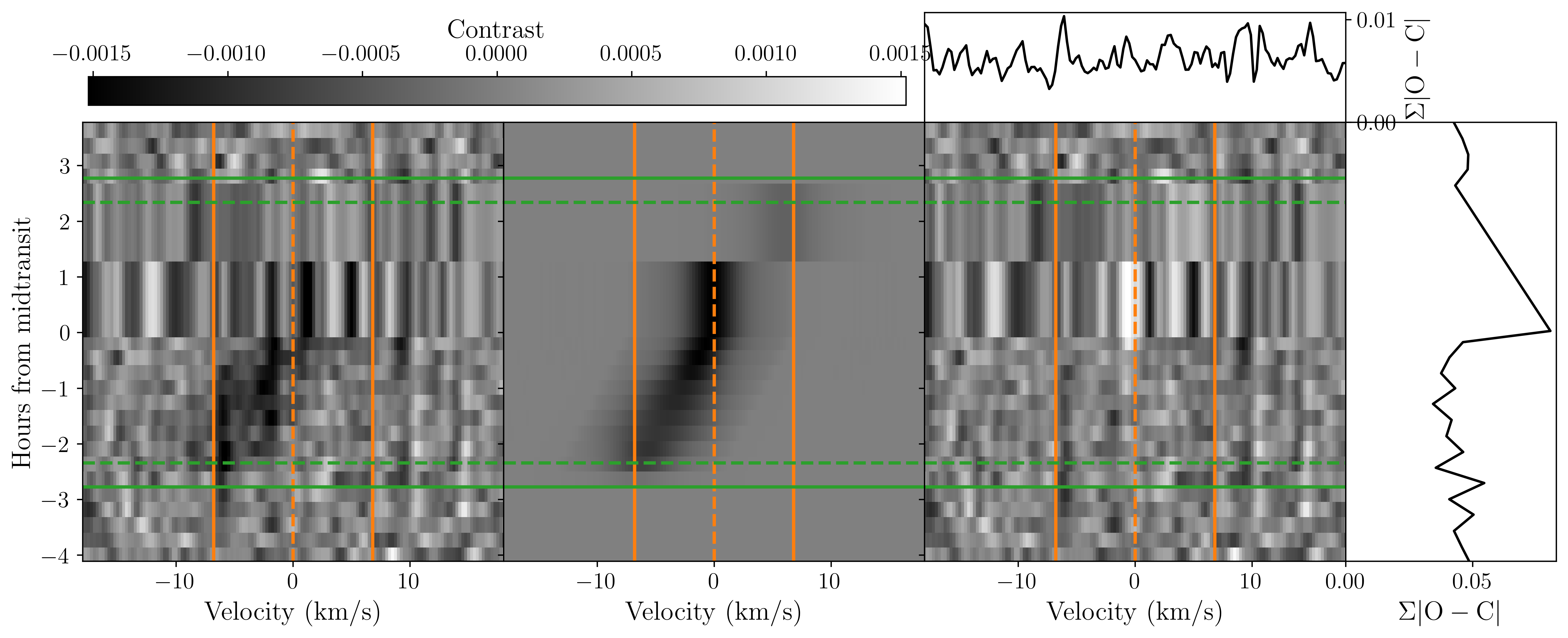
Figure 15: Doppler shadow for TOI-892. Same as in Fig. 4, but for TOI-892.

4.11 TOI-1130

TOI-1130 is a K dwarf with two transiting planets, an inner Neptune and an outer Jupiter, discovered by Huang et al. (2020). We used ESPRESSO to observe a transit of the larger planet, TOI-1130 c, on the night starting on June 1, 2021. The observations were carried out from around UT 01:30 to 06:00 on June 2, 2021. We opted for an exposure time of 660 s, yielding a sampling time of 701 s. TOI-1130 was observed by TESS in Sector 13 in 30-minute cadence and in Sectors 27 and 67 in 20-second cadence. The TESS light curve for planet c is shown in Fig. 40.

Because the planets in TOI-1130 are in or near a 2:1 mean-motion resonance, the planets show relatively large transit timing variations (TTVs). The TTV amplitudes are on the order of a few hours for planet b and 15 min for planet c (Korth et al., 2023). Based on the comprehensive model of the system developed by Korth et al. (2023), the mid-transit time of planet c on June 2, 2021 should have occurred at BJD $2459367.6304\pm 0.0003$ d (J. Korth, private communication). We used this result as a Gaussian prior on $T_{0}$ in our analysis.

The TTVs also affect the phase-folding process that is part of the construction of a high-SNR light curve. To deal with the TTVs, we identified the transits of both planet b and c in the TESS data, and fitted a model the TESS data alone, holding fixed all of the parameters except for the individual mid-transit times. Then, in our RV-RM analysis, we fitted the TESS data jointly with the RV time series while applying Gaussian priors on the mid-transit times with a width of $0.005$ d. We also applied a Gaussian prior on the stellar mean density of $\rho_{\star}=2.98\pm 0.18$ g cm^-3 (Korth et al., 2023). Most of the transits of planet b were irrelevant, but there was one instance of overlapping transits of planets b and c.

Our BF analysis gave a lower projected rotation velocity for TOI-1130 ($1.3$ km s^-1) than we found in the literature ($4.0\pm 0.5$ km s^-1, Huang et al., 2020). Our result is more in line with the upper limit of 3 km s^-1 reported by Korth et al. (2023). From the RV-RM analysis, we obtained $v\sin i_{\star}$ $=1.3\pm 0.5$ km s^-1 and $\lambda=$ $4_{-6}^{+5}$^∘ when applying a uniform prior on $v\sin i_{\star}$. With a Gaussian prior on $v\sin i_{\star}$, we obtained $\lambda=$ $4^{+5}_{-6}$^∘, which we regard as the best estimate. We need to stress that the accuracy of the result does depend on the prior on $T_{0}$ that was obtained from the model of (Korth et al., 2023).

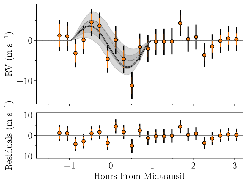
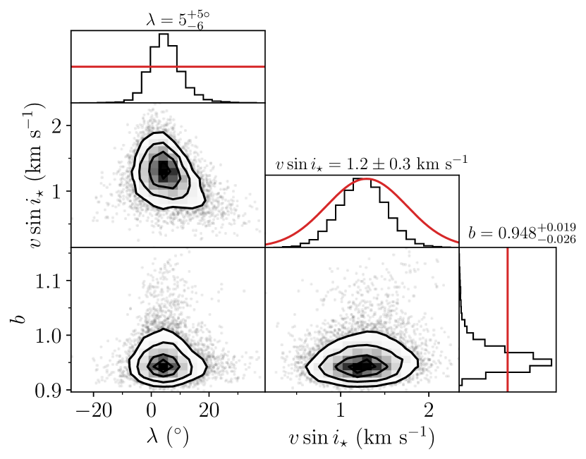
Figure 16: The RV-RM effect for TOI-1130. Same as for Fig. 2, but with RVs from ESPRESSO.

We investigated the subplanetary velocities for TOI-1130 to see if we could properly trace the deformation of the stellar lines for this grazing transit, where (unlike for K2-287) the planet only obscures part of the stellar limb. It proved more difficult to locate the distortion in the first and last few in-transit spectra, as shown in Fig. 17. We also found it necessary to adopt a Gaussian prior on $v\sin i_{\star}$.

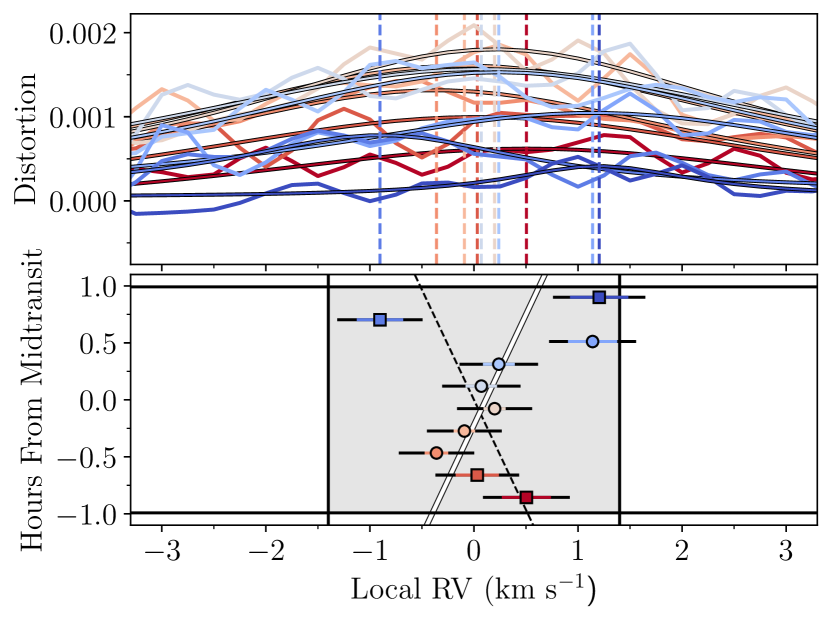
Figure 17: Subplanetary velocities for TOI-1130. In the top panel the distortion from subtracting the in-transit CCF from the out-of-transit are shown as colored (wiggly) lines. Lines of corresponding colors with a black outline are (Gaussian) fits to the distortion in order to extract the position of the distortion denoted by the dashed vertical line. The bottom panel shows the location of the distortion plotted around the midtransit time. The squares denote epochs for which the decrease in flux from the transiting planet is less than 0.75%. The solid white (black dashed) line shows a model for an (anti-)aligned configuration.

When fitting the subplanetary velocities using all of the data, the posterior for $\lambda$ had a peak centered on $0^{\circ}$, and a secondary peak near $\lambda=180^{\circ}$. We found the secondary peak to be a consequence of including the noisiest data points from the first and last few in-transit spectra. Out of concern over systematic errors in our model for limb-grazing transits, we repeated the fit after omitting the in-transit data that were obtained when the loss of light was smaller than 0.75% (the square data points in Fig. 17). The result was $\lambda=$ $6^{+10}_{-9}$^∘. Although excluding data without a firm justification is undesirable, we judge the evidence as indicating that any misalignment is smaller than about 20^∘.

4.12 WASP-50

WASP-50 is a G9 dwarf hosting a hot Jupiter on a $1.9$ d orbit discovered by Gillon et al. (2011). TESS data are available from observations in Sector 4 and 31 with 2 min and 20 sec cadence, respectively. Fig. 40 shows the TESS transit light curve.

On the night starting on August 24, 2022, we observed a transit of WASP-50 b with ESPRESSO. The observations started at around UT 05:10 and continued until UT 09:40 on August 25, 2022. An exposure time of 240 s ensured a cadence of 270 s.

The time series is well-sampled and the SNR is very high, exactly the case where we do not expect the results to be sensitive to the prior on $v\sin i_{\star}$. Indeed, for this system we found $-2.9\pm 1.2$^∘ when applying a uniform prior and $-2.9^{+1.2}_{-1.3}$^∘ for a Gaussian prior.

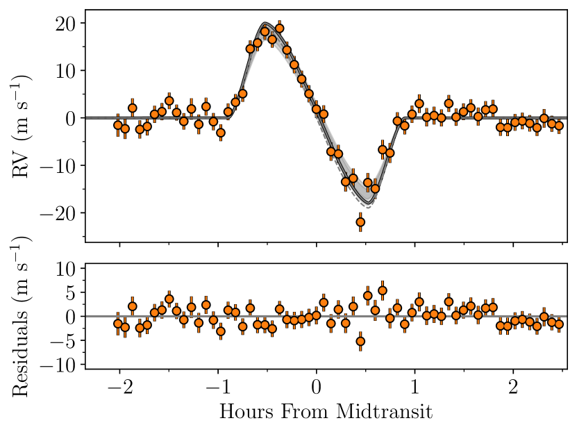
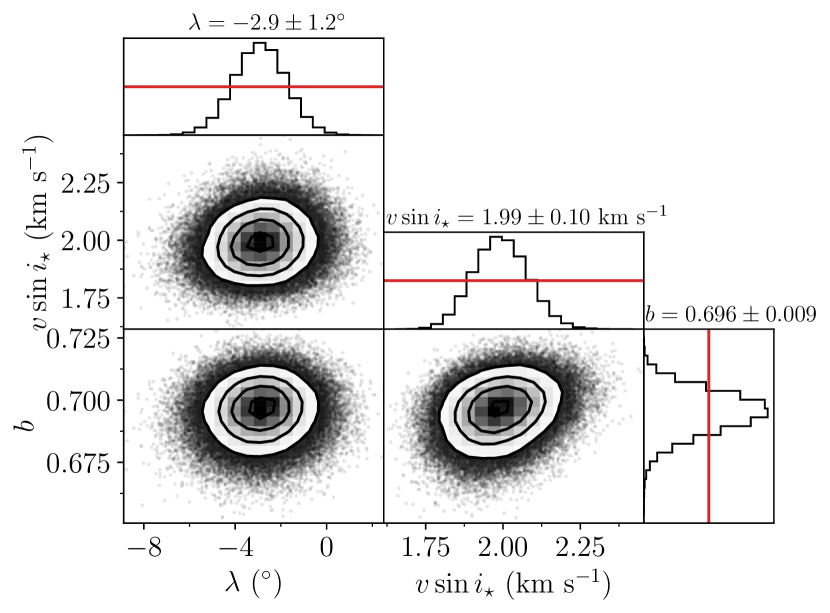
Figure 18: The RM-RV effect for WASP-50. Same as for Fig. 2, but with RVs from ESPRESSO.

The high-quality data prompted us to investigate the RM effect further. We examined the subplanetary velocitiesm, which were shown in Fig. 1, but in Fig. 19 we display them in a slightly different manner (similar to the format of Fig. 7 for K2-287). As was the case for K2-287, we included two jitter terms, one for when the planet’s silhouette is on or near the limb, and another when it is completely within the stellar disk. The result of our analysis using the subplanetary velocities was $v\sin i_{\star}$ $=2.77\pm 0.14$ km s^-1 and $\lambda=$ $-1.8\pm 1.0$^∘. The agreement with the RV-RM result is reassuring, but for our best estimate we chose the result $-2.9\pm 1.2$^∘ from the RV-RM analysis.

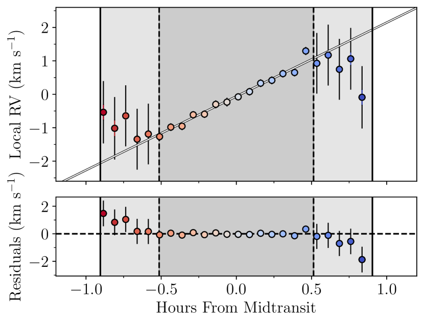
Figure 19: Subplanetary velocities for WASP-50. Subplanetary velocities for WASP-50 with color-coding as described in Fig. 1. The dark shaded area correspond to the time the planet is completely within the stellar disk and the light shaded area denote ingress and egress. The errorbars include a jitter term, where two separate terms have been added in quadrature; one for the epochs for the full transit and one for the epochs when the planet is partially outside of the limb of the star. The horizontal black lines in the top panel mark $v\sin i_{\star}$ from the fit.

4.12.1 Convective blueshift

This term “convective blueshift” refers to the net blueshift of the disk-integrated stellar spectrum caused by the imbalance in brightness between different components of convective cells. The upwelling gas is hotter, brighter, and blueshifted, while the sinking gas is cooler, fainter, and redshifted. Shporer & Brown (2011) showed that this effect contributes to the anomalous RVs with amplitudes of a few m s^-1, and variability on a timescale of several minutes. Within our sample, WASP-50 is the only system for which the quality of the data is high enough to contemplate detecting and modeling the convective blueshift.

We modelled the convective blueshift as described by Shporer & Brown (2011). In the model, the stellar disk is pixelated, and each pixel is assigned an intensity according to a limb-darkening law and a net convective velocity ($V_{\rm CB}$) directed toward the center of the star. The radial component of each blueshifted surface element is therefore $V_{\rm CB}\cos\theta$ where $\theta$ is the angle between the normal to the stellar surface and our line of sight. The value of $V_{\rm CB}$ is expected to range from about $-200$ m s^-1 for K-type stars to $-1000$ m s^-1 for F-type stars (Dravins & Nordlund, 1990a, b; Dravins, 1999). The solar value is about $-300$ m s^-1 (Dravins, 1987). Since WASP-50 is similar to the Sun, with $T_{\rm eff}=5400\pm 100$ K, a reasonable expectation is $V_{\rm CB}\approx-300$ m s^-1.

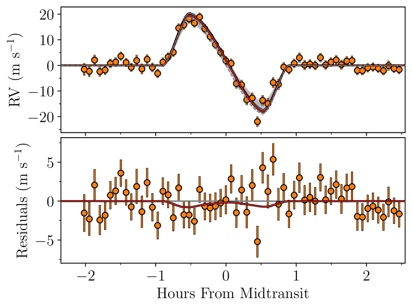
Figure 20: Convective blueshift in WASP-50. Same as the left panel of Fig. 18, but also showing a model as a red solid line that includes the effect of convective blueshift ($V_{\rm CB}=-300$ m s^-1).

Since the anomalous RV caused by the convective blueshift is smallest near the limb, and WASP-50 b has a high impact parameter ($b\approx 0.7$), the overall effect of the convective blueshift is expected to be rather weak, as shown in Fig. 20. Nevertheless, we tested whether the inclusion of the convective blueshift in our RV-RM model leads to a substantial improvement in the quality of the fit to the data,. We created a grid of $\lambda$ values between $-45^{\circ}$ and $+45^{\circ}$ in steps of $0.25^{\circ}$. For each choice of $\lambda$, we computed the Bayesian information criterion (BIC; Schwarz, 1978) for RV-RM models with and without the convective blueshift. The standard model has a minimum BIC for $\lambda=-2.9^{\circ}$ (as expected given our result of $-2.9\pm 1.2$^∘), whereas the model with the convective blueshift has a minimum BIC for $\lambda=-3.9^{\circ}$. The difference in the optimized BIC values is 4.5, favoring the model without the convective blueshift. We calculated the difference in BIC ($\Delta$BIC) between the two models at each $\lambda$. $\Delta$BIC changes sign around $\lambda=-4.9^{\circ}$ meaning that the net effect of including convective blueshift results in slightly lower (more misaligned) values for $\lambda$.

Even though we did not find that including the convective blueshift significantly improves the fit, we decided to repeat our RV-RM analysis after including the convective blueshift. For convenience, we did not jointly fit the TESS light curve; we simply held $b$, $R_{\rm p}/R_{\star}$, $P$, and $T_{0}$ fixed at the best-fit values from our previous run above. We applied a Gaussian prior on $V_{\rm CB}$ centered on $-400$ m s^-1 with a width of $100$ m s^-1. From this run we obtained $\lambda=-3.5\pm 1.3^{\circ}$ again suggesting a slightly more misaligned system. A smaller absolute value for $V_{\rm CB}$ (probably more in-line with the expected value for WASP-50) would make the difference in $\lambda$ from the two runs even smaller as such we do not expect convective blueshift to significantly affect the results. Thus, when attempting to measure $\lambda$ with a precision at the level of one degree, the results depend on how much one trusts the model for the convective blueshift and its assumed amplitude.

4.13 WASP-59

The WASP-59 system was discovered by Hébrard et al. (2013). The system consists of a warm Jupiter, WASP-59 b, orbiting a K-dwarf. We observed a transit of WASP-59 b with HIRES. The observations were carried out on November 23, 2016, starting at UT 05:19 to 09:46 with an exposure time of $787$ s. Including overhead the sampling time came out to $835$ s. The series of 20 observations spanned a transit.

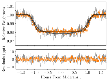
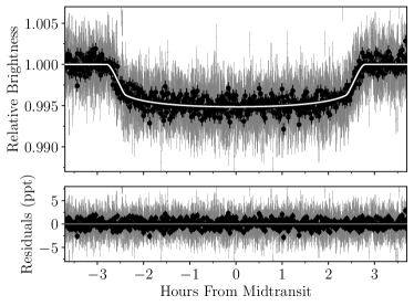
(a) WASP-59 b	(b) WASP-136 b
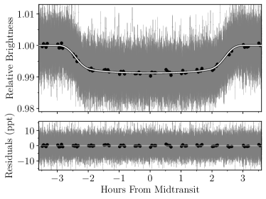
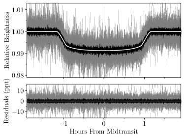
(c) WASP-172 b	(d) WASP-173Ab
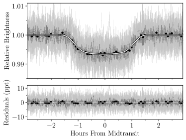
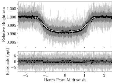
(e) WASP-186 b	(f) XO-7 b

Figure 41: Phasefolded light curves. Same as in Fig. 39. (a) WASP-59 b: TESS 2 min. cadence data shown in gray and ground-based 2 min. KeplerCam photometry in orange. (b) WASP-136 b: TESS 20 sec. and 2 min. cadence data shown in gray and black, respectively. (c) WASP-172 b: TESS 20 sec. and 30 min. cadence data shown in gray and black, respectively. (d) WASP-173Ab: TESS 20 sec. and 2 min. cadence data shown in gray and black, respectively. (e) WASP-186 b: TESS 20 sec., 2 min., and 30 min. cadence data are shown in light gray, gray, and black, respectively. (f) XO-7 b: TESS 20 sec., 2 min., and 30 min. cadence data are shown in light gray, gray, and black, respectively.

TESS observed the system in Sector 56 with a cadence of with a cadence of 2 min. Given the long time interval that elapsed between our HIRES observations and the TESS observations, one might be concerned about the extra uncertainty in the transit ephemerides. Fortunately, we also arranged for ground-based photometric observations of a transit a few weeks after our spectroscopic observation. We used KeplerCam, which is mounted on the 1.2 m telescope at the Fred L. Whipple Observatory on Mount Hopkins, Arizona (Szentgyorgyi et al., 2005). We observed with an $r^{\prime}$ filter on the night starting that began on the night of December 8, 2016. The light curves are shown in Fig. 41.

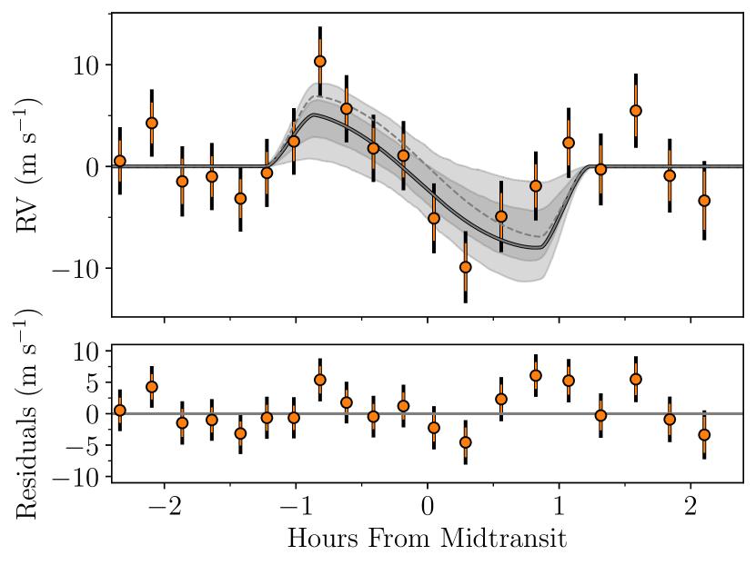
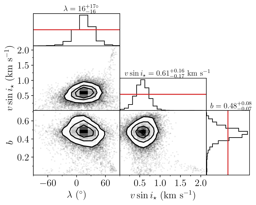
Figure 21: The RM-RV effect for WASP-59. Same as for Fig. 2, but with RVs from HIRES.

Because the HIRES spectra were imprinted with iodine absorption lines, we did not derive a value for $v\sin i_{\star}$ with the BF method. Instead, we adopted the value of $2.3\pm 1.2$ km s^-1 reported by Hébrard et al. (2013). When using this result as a Gaussian prior, we obtained $\lambda=$ $16^{+17}_{-16}$^∘ and $v\sin i_{\star}$ $=$$14.8\pm 0.5$ km s^-1, clearly suggesting that the Gaussian prior is not particularly informative. Indeed assuming a uniform prior on $v\sin i_{\star}$ we got $v\sin i_{\star}$ $=$$11^{+4}_{-11}$ km s^-1 and $\lambda=$ $16^{+18}_{-16}$^∘, which we adopt as a out final value for $\lambda$. The resulting RM curve and posteriors are shown in Fig. 21.

4.14 WASP-136

WASP-136 b is an inflated hot Jupiter orbiting an F9 subgiant star. The system was discovered by Lam et al. (2017). TESS data are available with 2-min cadence in Sector 29 and 20-sec cadence in Sector 41. The light curve is shown in Fig. 41.

We observed a transit with FIES on the night starting August 30, 2021, with observations running from UT 23:00 to UT 05:50 August 31, 2021. We opted for an exposure time of 1140 s, yielding a sampling time of 1320 s.

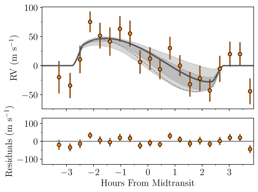
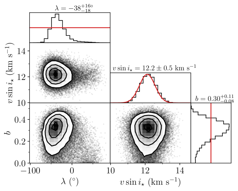
Figure 22: The RV-RM effect for WASP-136. Same as for Fig. 2. Here also with RVs from FIES.

Both of the RV-RM fits resulted in a significant misalignment for the WASP-136 system. We obtained $\lambda=$ $-57^{+9}_{-14}$^∘ when applying a uniform prior on $v\sin i_{\star}$, and $-38^{+16}_{-18}$^∘ when applying a Gaussian prior. We adopt the latter as our best estimate of the projected obliquity.

4.15 WASP-148

The WASP-148 system was discovered by Hébrard et al. (2020). The system consists of two giant planets orbiting a late-G dwarf with strong TTVs. The inner planet, WASP-148 b, is a transiting hot Jupiter with a period of 8.8 days. The star’s projected obliquity with respect to the orbit of planet b was measured by Wang et al. (2022) to be $\lambda=-8^{+9}_{-10}$^∘.

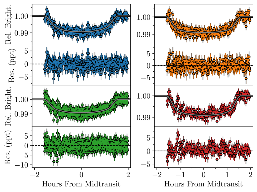
Figure 42: Phasefolded light curves of WASP-148 b. The MuSCAT-2 photometry obtained simultaneous with our spectroscopic transit observations. The observations in the different $griz$ filters are shown as blue, orange, green, and red markers, respectively.

We observed a transit of WASP-148 b using HARPS-N on the night starting March 21, 2021, with observations starting around UT 01:45 to 06:15 March 22, 2021. The exposure time was set to 900 s, resulting in a sampling time of 920 s. Because the strong TTVs lead to extra uncertainty in the transit ephemerides, we also arranged for simultaneous photometric observations of the transit with the Multicolor Simultaneous Camera for studying Atmospheres of Transiting exoplanets (MuSCAT-2; Narita et al., 2015) mounted on the Telescopio Carlos Sánches, Tenerife, Spain. MuSCAT-2 allows for simultaneous observations in four filters; we used a $griz$ filter set. The light curves, after detrending, are shown in Fig. 42. When modeling these light curves, we did not use GP regression. The limb-darkening coefficients tabulated by Claret et al. (2013) for these filters and for the appropriate stellar parameters are reproduced in Table 7.

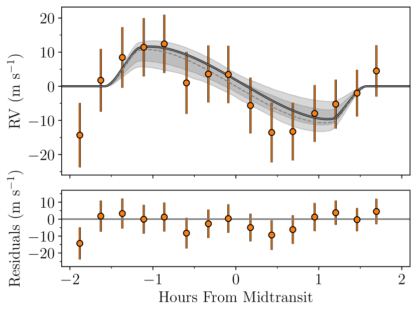
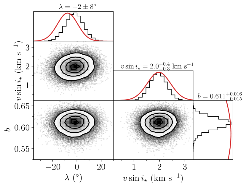
Figure 23: WASP-148. Same as for Fig. 2, but with RVs from HARPS-N.

At first, we fitted the RM effect for this system jointly with the TESS and MuSCAT-2 light curves, allowing the mid-transit time of each transit to be a freely adjustable parameter (as we did for TOI-1130, Section 4.11). We also tried fitting only the MuSCAT-2 light curves and not the TESS light curve. In both cases, we found $\lambda=16\pm 40^{\circ}$, which is consistent with, but less precise than, the measurement reported by Wang et al. (2022).

Almenara et al. (2022) performed a “photodynamical” analysis of the system, in which the light curve is fitted with a model in which all the mutual gravitational interactions between the star and both planets are taken into account. They used the data presented by Hébrard et al. (2020) along with additional ground-based data and TESS data. Given their comprehensive modeling effort, we decided to use the parameters from Almenara et al. (2022) as priors, and fitted only the HARPS-N RV measurements and the MuSCAT-2 light curve. The free parameters relevant to the light curve were the mid-transit time, $a/R_{\star}$, $\cos i$, $R_{\rm p}/R_{\star}$, and the sum-of-limb-darkening coefficients for each filter. The period was held fixed. In addition, we included a Gaussian prior on the projected obliquity using the value of $\lambda=-8^{+9}_{-10}$^∘ as to incorporate all the information available for the system. Again, we performed two MCMCs obtaining a value of $-2\pm 8$^∘ for both the run with a uniform and the one with a Gaussian prior on $v\sin i_{\star}$, respectively.

Table 7: WASP-148, photometry only.

Parameter	Value	Prior
$T\rm_{0}\ (BJD)$	$2459295.6598\pm 0.0002$	$\mathcal{U}(2459295,2459296)$
$a/R_{\star}$	$19.7^{+0.4}_{-0.3}$	$\mathcal{U}(10,30)$
$R_{\mathrm{p}}/R_{\star}$	$0.0853^{+0.0008}_{-0.0007}$	$\mathcal{U}(0,1)$
$q_{1}+q_{2}:g$	$0.97\pm 0.05$	$\mathcal{N}(0.781,0.1)$
$q_{1}+q_{2}:i$	$0.78\pm 0.06$	$\mathcal{N}(0.613,0.1)$
$q_{1}+q_{2}:r$	$0.83\pm 0.05$	$\mathcal{N}(0.698,0.1)$
$q_{1}+q_{2}:z_{s}$	$0.60\pm 0.06$	$\mathcal{N}(0.547,0.1)$
$\cos i$	$0.011_{-0.011}^{+0.004}$	$\mathcal{U}(0.0,0.5)$
Filter	$q_{1}$	$q_{2}$
$g$	0.73	0.05
$r$	0.53	0.17
$i$	0.40	0.22
$z_{s}$	0.23	0.32

• Top: Results from an MCMC using only the MuSCAT-2 photometry for the transit of WASP-148 b. Bottom: The limb-darkening coefficients for each filter using Claret et al. (2013).

As this is a dynamically interesting system, for which a large collection of transit times over a long interval can help to constrain the parameters of the planetary system, we measured the mid-transit time based on a fit solely to the MuSCAT-2 light curves. The results are given in Table 7.

4.16 WASP-172

WASP-172 is an F star with a bloated hot Jupiter discovered by Hellier et al. (2019a). Data from TESS are available with 30-min cadence from Sector 11 and 20-sec cadence from Sectors 37 and 38. The TESS light curve is shown in Fig. 41.

On the night starting June 1, 2022, we observed a transit using ESPRESSO with observations being carried out from UT 23:00 to UT 06:40. We opted for an exposure time of 900 s, resulting in a sampling time of 940 s. The RVs are shown in Fig. 24, where three data points are marked with gray points as they were excluded from the analysis, since they were taken at high airmass.

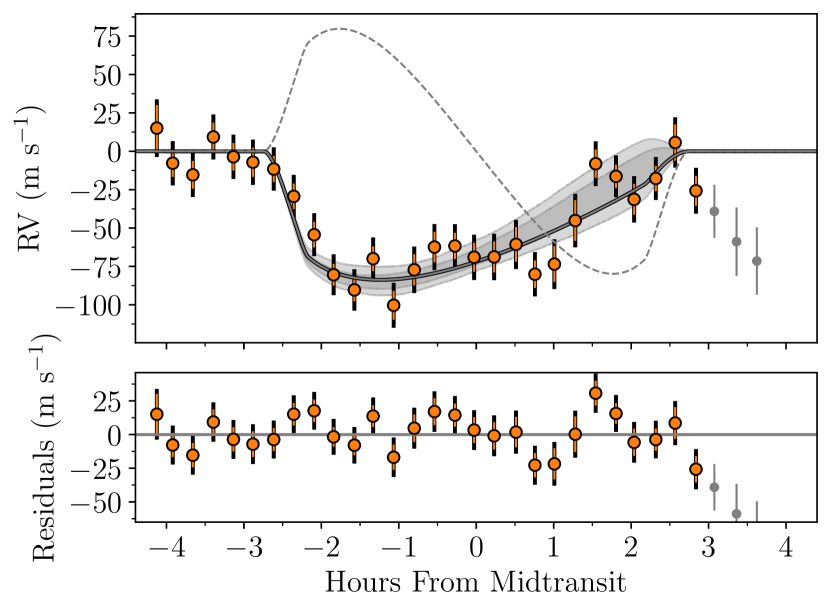
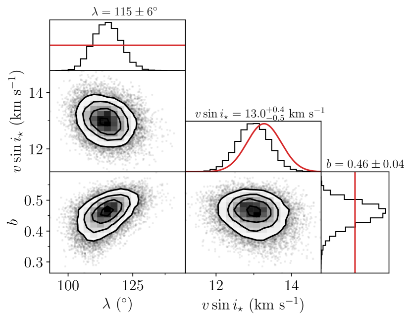
Figure 24: WASP-172. Same as for Fig. 2, but with RVs from ESPRESSO. The gray data points were excluded in the fit due to high airmass.

By fitting the RV-RM effect and the TESS light curve, we found $\lambda=$ $118\pm 6$^∘ and $115\pm 6$^∘ for $\lambda$ when applying a uniform prior or a Gaussian prior on $v\sin i_{\star}$, respectively. Given the high quality of the data, and the relatively rapid rotation of the star ($v\sin i_{\star}$ $=$$13.0^{+0.4}_{-0.5}$ km s^-1), we decided to analyze the Doppler shadow. The results are displayed in Fig. 25. The Doppler-shadow analysis gave $\lambda=$ $121^{+11}_{-13}$^∘, consistent with the RV-RM results. We adopted $115\pm 6$^∘ as our best estimate for $\lambda$, based on the RV-RM fit with a Gaussian prior on $v\sin i_{\star}$.

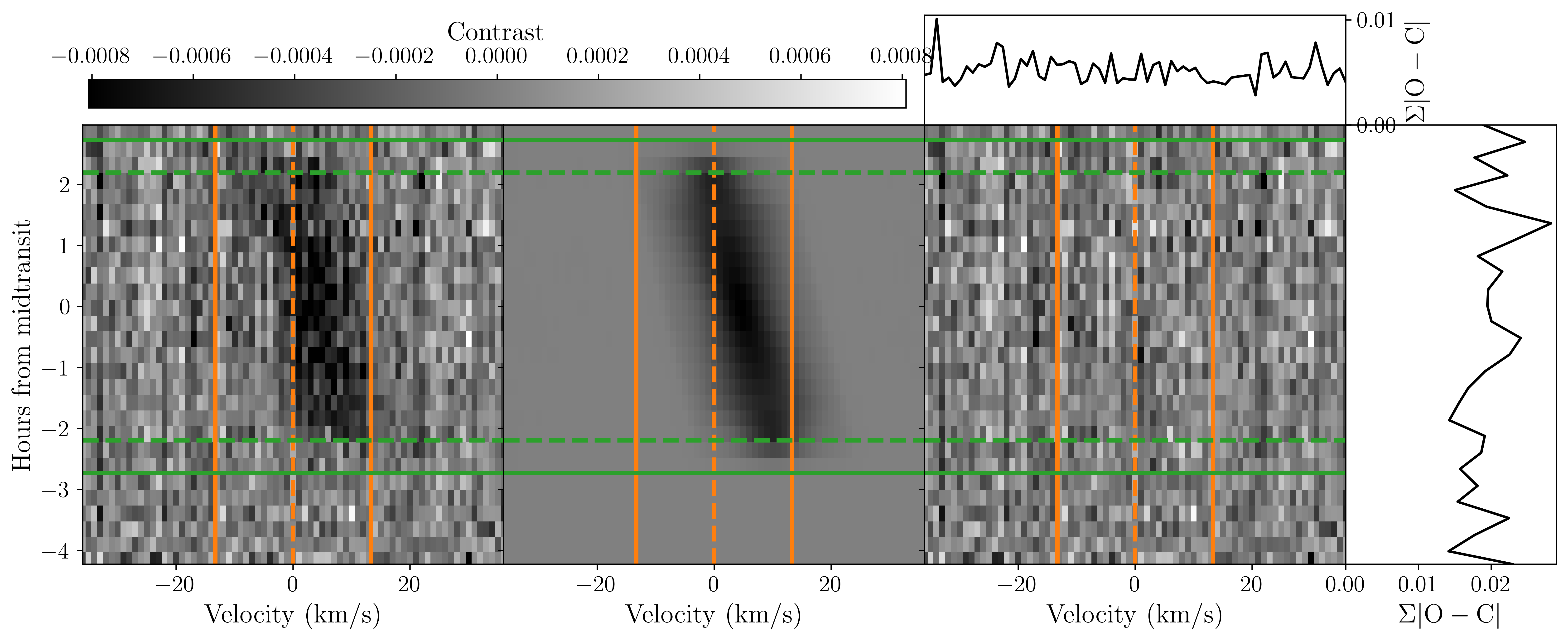
Figure 25: Doppler shadow for WASP-172. Same as in Fig. 4, but for WASP-172.

The ESPRESSO transit spectroscopy presented here was also used by Seidel et al. (2023) in an investigation of the planet’s atmosphere. They reported the detection of sodium and hydrogen absorption, as well as a tentative detection of iron absorption. In their study, a value of $\lambda=121\pm 13^{\circ}$ was adopted to correct for the RM effect, which was taken from our Doppler-shadow analysis prior to the completion of this paper.

4.17 WASP-173A

WASP-173Ab is a hot Jupiter discovered by Hellier et al. (2019a). The host star is of spectral type G3V and has a wide-orbiting stellar companion. The planet was also dubbed KELT-22Ab by Labadie-Bartz et al. (2019), who reported an independent discovery of the transits using data from the KELT data. Here, we use the name WASP-173Ab.

TESS observed the system twice. Data with 2-min cadence are available from Sector 2, and with 20-sec cadence from Sector 29. The TESS light curve is shown in Fig. 41. We observed a transit on the night starting July 23, 2022, with observations beginning at UT 05:40 until UT 10:00. The exposure time was set to 555 s, yielding a sampling time of 590 s. The RVs are shown to the left in Fig. 26.

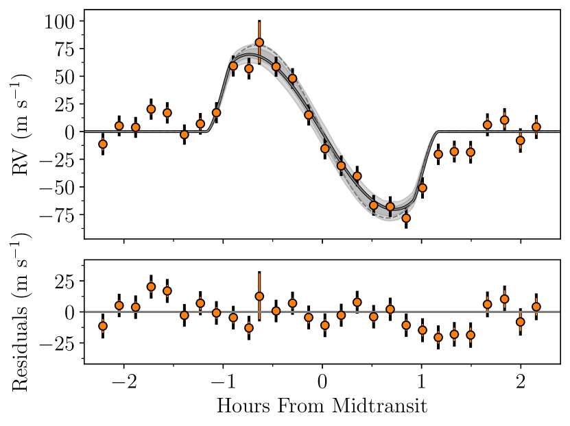
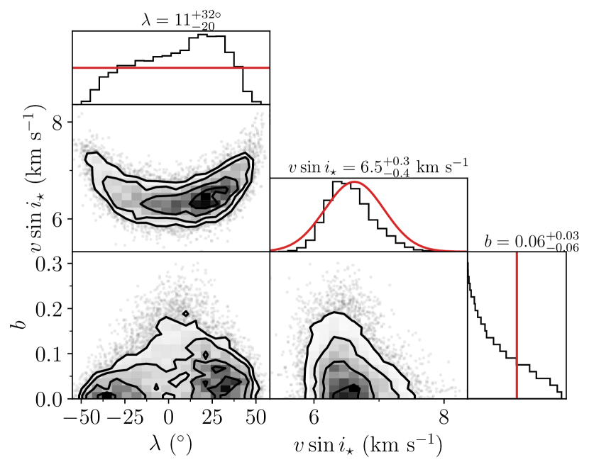
Figure 26: The RV-RM effect for WASP-173A. Same as for Fig. 2, but with RVs from ESPRESSO.

Our analysis followed similar steps as for WASP-172 (see the previous section). We performed the usual RV-RM analyses and also an analysis of the Doppler shadow, for which the results are shown in Fig. 27. The RV-RM results were $\lambda=$ $16^{+38}_{-31}$^∘ when applying a uniform prior on $v\sin i_{\star}$ and $11^{+32}_{-20}$^∘ for a Gaussian prior, while the shadow run resulted in a value for $\lambda$ of $25_{-11}^{+12}$^∘.

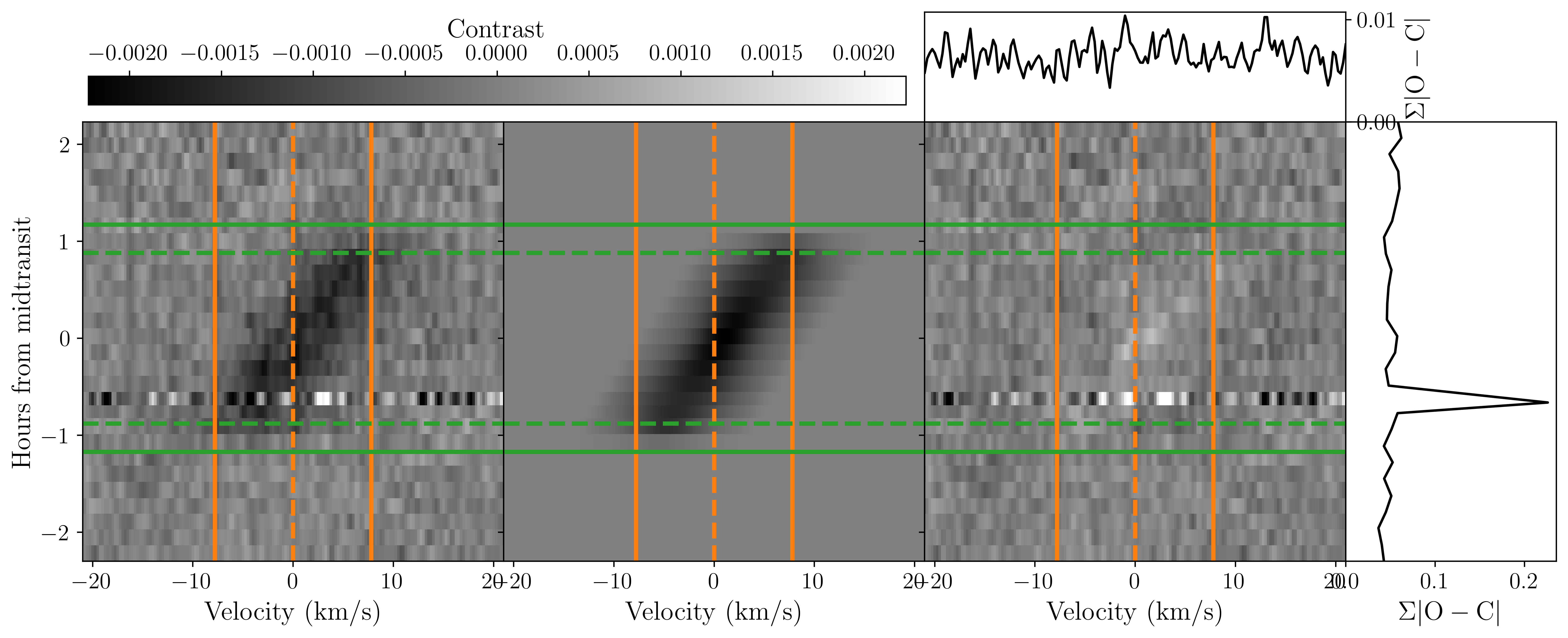
Figure 27: Doppler shadow for WASP-173A. Same as in Fig. 4, but for WASP-173A.

The $v\sin i_{\star}$ derived from the Doppler-shadow analysis was $7.2^{+0.4}_{-0.4}$ km s^-1, which is a bit higher than the results obtained from the RV-RM anlayses ($6.6_{-0.8}^{+0.6}$ km s^-1) and a Gaussian prior ($6.5^{+0.3}_{-0.4}$ km s^-1). The RV-RM-based values are closer to the value derived from the BF of 6.6 km s^-1. As our best estimate of $\lambda$, we therefore adopt the value of $11^{+32}_{-20}$^∘ from our run applying a Gaussian prior on $v\sin i_{\star}$.

4.18 WASP-186

Schanche et al. (2020) discovered the WASP-186 b, a massive hot Jupiter with an eccentric orbit around a mid-F star. As noted by Schanche et al. (2020), WASP-186 was observed by TESS in Sector 17 and produced data with a 30-min cadence. In addition, TESS observed this system in Sectors 42 and 57 and the data are available with 2-min and 20-sec cadence, respectively. The light curves are shown in Fig. 41.

Using FIES, we observed a transit on the night October 11, 2021, with observations starting UT 22:30 and continuing until UT 02:50 October 12, 2021. The exposure time was set to 900 s, and the time between mid-exposures was 1080 s. The transit observations are shown in Fig. 28.

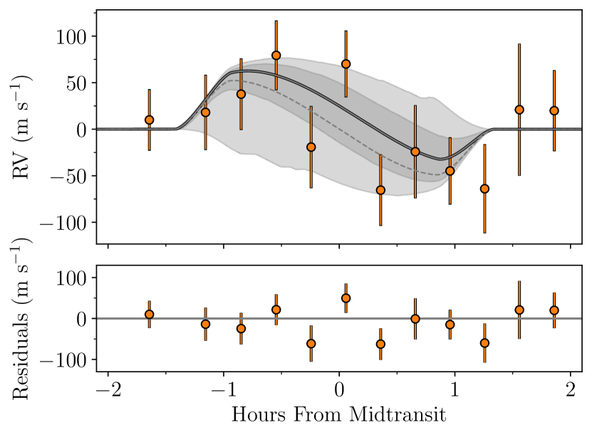
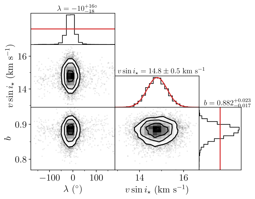
Figure 28: The RV-RM effect for WASP-186. Same as for Fig. 2. Here also with RVs from FIES.

Our two RV-RM fits gave $\lambda=$ $-10^{+29}_{-32}$^∘ and $\lambda=$ $-10^{+18}_{-16}$^∘ for the run with a uniform and the one with a Gaussian prior on $v\sin i_{\star}$, respectively. The values are in agreement and the prior on $v\sin i_{\star}$ leads to a more precise result for $\lambda$. Therefore, we chose $\lambda=$ $-10^{+18}_{-16}$^∘ as our best estimate for WASP-186.

4.19 XO-7

XO-7 b was discovered by Crouzet et al. (2020) as part of the XO project (McCullough et al., 2005). The transiting planet is a hot Jupiter. There is also a massive companion on an orbit with a period of at least 2 years around the G2V host star (Crouzet et al., 2020). TESS data are available with 30-min cadence in Sectors 18, 19, and 20; with 2-min cadence in Sectors 40, 47, 53, 53; and with 20-sec cadence in Sectors 59 and 60. The TESS light curves are shown in Fig. 41.

We observed a transit of XO-7 b with FIES on the night starting on August 27, 2022, with observations starting around UT 00:15 and continuing until 04:00 August 28, 2022. We opted for an exposure time of 840 s, resulting in a sampling time of 1000 s. The RVs from the transit night are shown in Fig. 29. The egress was not completely covered, and no observations were made after the egress.

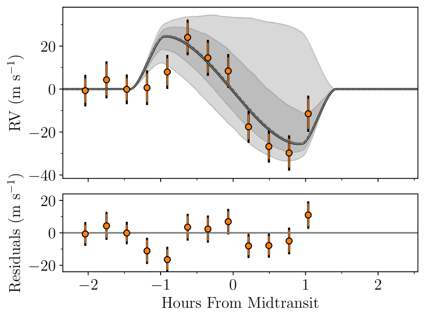
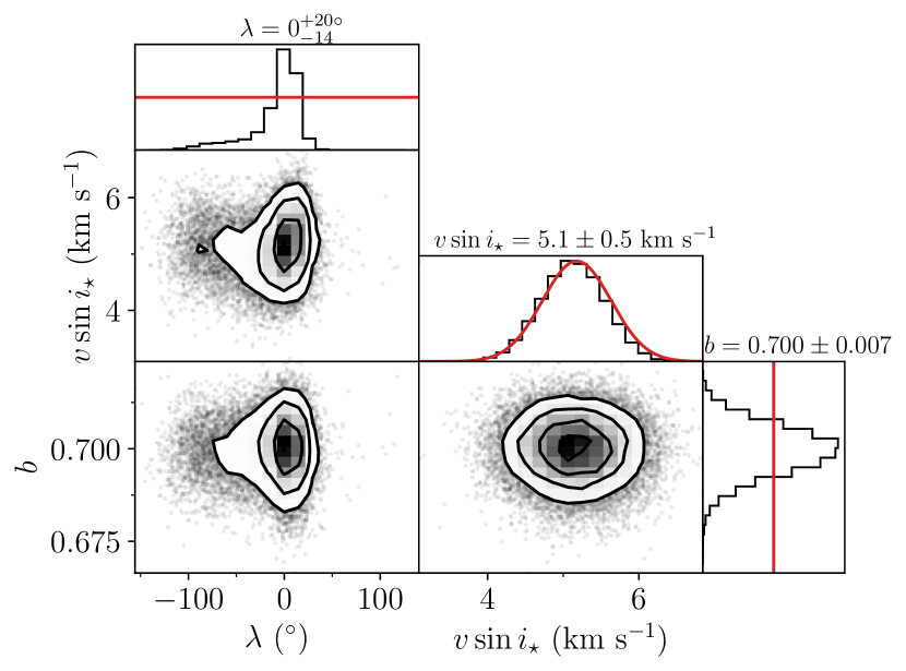
Figure 29: The RV-RM effect for XO-7. Same as for Fig. 2. Here also with RVs from FIES.

The RV-RM results for $\lambda$ are $-4^{+27}_{-23}$^∘ and $0^{+20}_{-14}$^∘ for the runs with a uniform and a Gaussian prior on $v\sin i_{\star}$, respectively, with the posterior distribution for the latter case shown in Fig. 29. Despite the incomplete coverage of the transit, the high impact parameter of $b\sim 0.7$ enabled decent constraints to be placed upon $\lambda$.

The posterior for $\lambda$, shown on the right side of Fig. 29, has a tail on the left side extending toward $-90^{\circ}$, allowing for the possibility that system is strongly misaligned. This tail is probably caused by the lack of egress/post-egress observations and also shows up in the 2$\sigma$ contours in the left panel of Fig. 29. We wondered if this unusual feature is related to the lack of egress and post-egress observations. We investigated the issue by examining the stacked spectral CCFs. The stacked CCFs showed contours that largely agree with the posteriors from our RV-RM. However, a peak is seen at around ($v\sin i_{\star}$,$\lambda$)=($4$ km s^-1,$-60^{\circ}$) that is more consistent with the negative tail of the posterior from the RV-RM analysis, favoring a more misaligned system. A second and more complete transit observation seems warranted. For now, we adopted $0^{+20}_{-14}$^∘ as our best estimate, based on the run with a Gaussian prior on $v\sin i_{\star}$.

4.20 WASP-26

WASP-26 b is a hot Jupiter orbiting an early G-type star, discovered by Smalley et al. (2010). Albrecht et al. (2012b) analyzed the RV-RM effect based on data obtained with the Planet Finder Spectrograph (PFS; Crane et al., 2010) mounted at the 6.5 m Magellan II telescope. The RV time series is shown in the left half of Fig. 30. They reported $\lambda=-34^{+36}_{-26}$^∘.

This case is unlike all of other cases presented in this paper in that we did not obtain any new data. Rather, we wanted to take advantage of TESS data that did not exist at the time of the prior study, and correct an error that was made in the prior study. The error was the adoption of an incorrect prior constraint on the transit duration ($T_{12}$, in the terminology of Albrecht et al. 2012b), which can be seen in their Table 3. This error resulted in an incorrect value of $b$ that affected the results for $\lambda$.

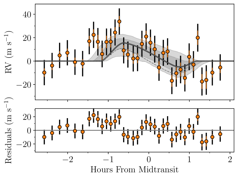
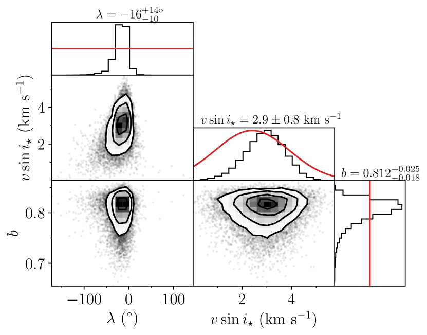
Figure 30: The RV-RM effect for WASP-26. Same as for Fig. 2, but with RVs from PFS.

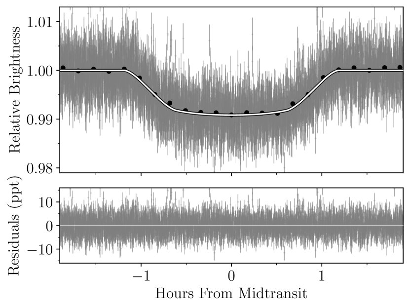
Figure 43: Phasefolded light curve of WASP-26 b. Unbinned 20 sec. cadence data are shown in gray and in black the binned ($\sim$6 min.) data are shown.

Rather than placing a prior on $T_{21}$, we followed our usual procedure of fitting the TESS light curve jointly with the RVs. We used TESS 20-sec data from Sector 29, shown in Fig. 43). As in Albrecht et al. (2012b), we applied a Gaussian prior on $v\sin i_{\star}$ of $2.4\pm 1.5$ km s^-1, and as usual, we applied Gaussian priors on the macro- and microturbulent velocities of $4.0\pm 1.0$ km s^-1 and $1.1\pm 1.0$ km s^-1, respectively. We also applied a Gaussian prior on $T_{0}$ taken from Anderson et al. (2011), as did Albrecht et al. (2012b). The reason for this choice is that about 10 years elapsed between the spectroscopic transit observations and the TESS observations; small systematic uncertainties in the TESS-based ephemeris might propagate into large uncertainties in the relevant transit time. We found a projected obliquity of $-16^{+14}_{-10}$^∘. Fig. 30 shows the RV-RM curve and posteriors.

4.21 Results

Table 8 gives our best estimates of $\lambda$ and $v\sin i_{\star}$ for each system. For cases in which the rotation period could be measured, the table also includes the stellar inclination, $i_{\star}$, calculated as per Masuda & Winn (2020), and the true obliquity. Other key parameters are given in Table 9.

Table 8: Final results for $v\sin i_{\star}$, $\lambda$, $i_{\star}$, and $\psi$.

System	$v\sin i_{\star}$ a	$\lambda$	$i_{\star}$	$\psi$
	(km s-1)	(∘)	(∘)	(∘)
HD 118203	$4.9^{+0.4}_{-0.5}$	$-23^{+25}_{-38}$	$17\pm 2$	$75^{+3}_{-5}$
HD 148193	$6.3\pm 0.4$	$14^{+7}_{-8}$	…	…
K2-261	$1.3\pm 0.4$	$32^{+48}_{-33}$	…	…
K2-287	$1.16\pm 0.17$	$23^{+12}_{-13}$	…	…
KELT-3	$7.2\pm 0.4$	$-5\pm 4$	…	…
KELT-4A	$5.8_{-0.5}^{+0.4}$	$80_{-22}^{+25}$	…	…
LTT 1445Ab	$1.4\pm 0.5$	$22_{-83}^{+98}$	…	…
TOI-451Ab	$8.1\pm 0.5$	$-23^{+37}_{-40}$	$69^{+11}_{-8}$	$40^{+22}_{-28}$
TOI-813	$8.4\pm 0.5$	$-32\pm 23$	…	…
TOI-892	$6.5\pm 0.5$	$-12^{+18}_{-16}$	…	…
TOI-1130	$1.2\pm 0.3$	$4^{+5}_{-6}$	…	…
WASP-50	$1.97\pm 0.10$	$-2.9\pm 1.2$	…	…
WASP-59	$0.58^{+0.18}_{-0.16}$	$16^{+18}_{-16}$	…	…
WASP-136	$12.2\pm 0.5$	$-38^{+16}_{-18}$	$38^{+7}_{-6}$	$60\pm 8$
WASP-148	$2.0^{+0.4}_{-0.3}$	$-2\pm 8$	$68^{+8}_{-21}$	$21^{+9}_{-17}$
WASP-172	$13.0^{+0.4}_{-0.5}$	$115\pm 6$	$73^{+9}_{-14}$	$112\pm 6$
WASP-173A	$6.5^{+0.3}_{-0.4}$	$11^{+32}_{-20}$	$71^{+10}_{-13}$	$30\pm 14$
WASP-186	$14.8\pm 0.5$	$-10^{+18}_{-16}$	$75^{+7}_{-15}$	$22^{+11}_{-14}$
XO-7	$5.1\pm 0.5$	$0^{+20}_{-14}$	$14.5^{+1.6}_{-1.4}$	$70\pm 1.7$
WASP-26	$2.9\pm 0.8$	$-16^{+14}_{-10}$	…	…

• In general the $v\sin i_{\star}$ value is largely constrained by the Gaussian prior of $\sigma=0.5$ km s^-1 applied.

• We caution that we might not have detected the RM effect in these systems and these measurements are therefore dubious.

5 Discussion

We now return to the four questions posed in the introduction about the distribution of obliquities of stars with transiting planets. We combined the $\lambda$ measurements presented in this paper (and listed in Table 8) with those measured previously. Specifically, we used the catalog assembled by Albrecht et al. (2022) with the help of the TEPcat catalog (Southworth, 2011), and several other measurements that have appeared in the more recent literature (up until February 26th, 2024). Table LABEL:tab:lamlit gives the key parameters for these additional systems, along with the systems presented in this study. Fig. 31 shows plots of $\lambda$ and $\psi$ as a function of $T_{\rm eff}$, $a/R_{\star}$ and $M_{\rm p}/M_{\star}$.

As mentioned we excluded our results for LTT 1445Ab and TOI-451Ab in the ensemble analyses below. Furthermore as this study builds upon the sample presented in Albrecht et al. (2022) systems excluded in there are also excluded here (based on the criteria outlined in their Appendix A).

Figure 31: Obliquities and projected obliquities as a function of $T_{\rm eff}$ (left), $a/R_{\star}$ (center), and $M_{\rm p}/M_{\star}$ (right). Triangles indicate the a measurement whose value is outside of the plotted range. In all panels, the color of each data point conveys $T_{\rm eff}$ using the color scale shown in the lower left panel. The contours are KDEs illustrating the density of measurements in a given parameter space.

5.1 A Preference for Polar Planets?

Albrecht et al. (2021) investigated a sample of 57 systems for which $\psi$ has been determined by combining measurements of the projected obliquity ($\lambda$) and the stellar inclination angle ($i_{\star}$). Of the 19 values of $\psi$ that are inconsistent with $0^{\circ}$, 18 are between $80^{\circ}$ and $125^{\circ}$. They hypothesized that the misaligned systems show a preference for approximately polar orbits. Siegel et al. (2023) and Dong & Foreman-Mackey (2023) followed up by replicating the preceding work and analyzing the larger sample of systems for which only $\lambda$ has been measured but not $i_{\star}$. The larger sample did not show a significant preference for polar orbits, suggesting that the sample analyzed by Albrecht et al. (2021) was somehow biased toward polar orbits.

We revisited the issue with a sample that is about 40% larger. The current tally of systems with $\lambda$ measurements is 205, of which $\psi$ is known for 87. In the analysis that follows, when considering the $\psi$ measurements, we decided to omit the 6 systems for which the gravity-darkening technique was employed, because parameter degeneracies make it difficult to measure $\psi$ when it is near $0^{\circ}$, $90^{\circ}$, or $180^{\circ}$. When considering only the $\lambda$ measurements, we retained the 6 gravity darkening measurements.

First, we repeated the statistical tests performed by Albrecht et al. (2021) using the enlarged set of $\psi$ measurements. We selected the 27 systems for which $\cos\psi<0.75$ and computed two statistics that quantify clustering: the dispersion around $\cos\psi=0$ and the standard deviation relative to the mean. We then used Monte Carlo simulations to find the probability of obtaining clustering statistics at least as large as those that were observed if the obliquities were drawn from an isotropic distribution (i.e., a uniform distribution in $\cos\psi$). A subtlety of these calculations is that for given values of the observables $|\cos i|$ (from the transit impact parameter), $|\sin i_{\star}|$ (from rotational broadening) and $\lambda$ (from the RM effect), there are two closely-spaced solutions for $\psi$:

$$\cos\psi=|\sin i_{\star}\sin i|\,\cos\lambda\pm|\cos i_{\star}\cos i|.$$ (3)

Following Albrecht et al. (2021), our Monte Carlo simulations take this discrete degeneracy into account by randomly choosing one of the two solutions in each iteration. The results were $p=9.4\times 10^{-4}$ for the dispersion and $p=3.8\times 10^{-4}$ for the standard deviation. Applying the same test to the sample of 14 systems that were available to Albrecht et al. (2021) and were not based on gravity darkening gives $p=1.4\times 10^{-2}$ and $2.1\times 10^{-3}$, respectively. Thus, the inclusion of 13 new data points has reduced the $p$-values by factors of 15 and 5.5, allowing a firmer rejection of the null hypothesis.

Next, we used the “DFM” (Dong & Foreman-Mackey) code provided by Dong & Foreman-Mackey (2023) to fit a model to the obliquity data consisting of the sum of two Beta distributions, representing the aligned and misaligned populations. Each Beta distribution is characterized by three hyperparameters: a weight $w$, a mean $\mu$, and an inverse variance $\kappa$. We adopted the same priors on the hyperparameters as outlined in Dong & Foreman-Mackey (2023). Table 12 gives the results for the hyperparameters when the DFM code is applied to different samples of the data, and Fig. 32 shows the posterior probability density for $\cos\psi$.

The left panel of Fig. 32 shows the results of analyzing the complete sample of projected obliquity measurements. There is a strong peak at $\cos\psi=1$ representing the aligned systems, and a much broader distribution representing the misaligned systems. The distribution falls off toward retrograde systems ($\cos\psi<0.75$) but otherwise there is little or no evidence for a concentration near $\cos\psi=0$, in agreement with the findings by Dong & Foreman-Mackey (2023) and Siegel et al. (2023).

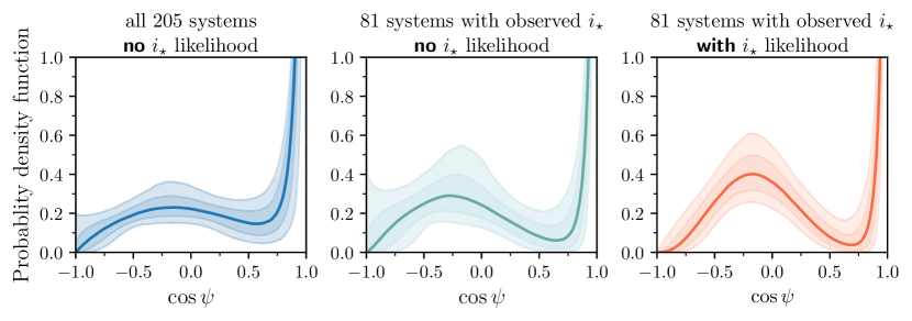
Figure 32: Hierarchical Bayesian inference of the obliquity distribution using the code of Dong & Foreman-Mackey (2023). The left panel is for all systems for which $\lambda$ was measured, the middle panel is for systems for which both $\lambda$ and $i_{\star}$ were measured but without using the $i_{\star}$ information, and the right panel is for systems for which both $\lambda$ and $i_{\star}$ were measured and making use of the $i_{\star}$ information.

The middle panel of Fig. 32 shows the results of analyzing only those systems for which constraints on $i_{\star}$ are available, but without using the $i_{\star}$ information to perform the inference. The inferred probability density of $\cos\psi$ does not look too different from the case described above.

The right panel of Fig. 32 shows the results of analyzing only those systems for which constraints on $i_{\star}$ are available, and using the $i_{\star}$ information to perform the inference. This is the type of sample that led Albrecht et al. (2021) to propose that there is a peak near $\cos\psi=0$, and indeed, we find a similar result.

The preceding results suggest that the obliquity distribution of the systems for which measurements of both $\lambda$ and $i_{\star}$ have been reported is different from that of the systems for which $\lambda$ was measured and no constraints are available on $i_{\star}$. This is true even though we have excluded inclination measurements obtained via gravity darkening, thereby eliminating the bias discussed by Siegel et al. (2023).

It is probably relevant that the $\lambda$ & $i_{\star}$ sample is enriched in the types of systems that are known to show frequent misalignments: sub-Saturns ($0.025$ M${}_{\rm J}<M_{\rm p}<0.2$ M_J), and hot Jupiters around hot stars ($a/R_{\star}<7$, $M_{\rm p}>0.3$ M_J, $T_{\rm eff}\geq 6250$ K). Stellar inclination measurements in those systems almost all come from the $v\sin i_{\star}$ method – the combination of a photometric rotation period, rotational Doppler broadening of the spectral absorption lines, and the stellar radius. In the entire sample, there are 17 sub-Saturns, of which inclination measurements are available for 11, of which 5 have $\cos\psi<0.75$. The entire sample also contains 41 hot Jupiters around hot stars, of which 15 have inclination measurements. After excluding the gravity-darkening measurements, we are left with 10 hot Jupiters, all of which have $\cos\psi<0.75$.

By combining the 5 misaligned hot Neptunes and the 10 misaligned hot Jupiters, we constructed a sample of 15 systems and subjected it to the same Monte Carlo experiments described above to test the null hypothesis that they are drawn from an isotropic distribution. For the dispersion-around-zero and standard deviation, we found $p=3.1\times 10^{-3}$ and $p=3.5\times 10^{-3}$, respectively. We also applied the DFM code to a sample consisting only of sub-Saturns, and a sample consisting only of hot Jupiters around hot stars, with results that are given in Table 12 and displayed in Fig. 33, in the same format as in Fig. 32. For the sub-Saturns, a central peak appears to be favored by the data, although the uncertainty in the distribution is large due to the small number of systems (17). A central peak is even more pronounced in the sample of hot Jupiters around hot stars (41 systems including the measurements employing the gravity darkening method). For the subset of systems with inclination measurements from this hot Jupiter sample, since all of the systems are misaligned, we modeled the distribution with a single Beta distribution rather than using two components. There is a clear peak at $\cos\psi\approx-0.2$ or $\psi\approx 100^{\circ}$. Indeed, all of these 10 systems are consistent with $\psi=90^{\circ}$ with varying degrees of uncertainty, and a simple kernel-density estimate of the distribution shows a peak at $\cos\psi=0$. Both distributions are shown in Fig. 33.

To investigate the importance of the priors assumed for the hyperparameters in the “DFM” code for these subpopulations, we tried adopting less informative priors on the variance, $\kappa$ or rather $\log\kappa$, hyperparameter. Here we tried a uniform prior instead of the Gaussian prior used in Dong & Foreman-Mackey (2023, i.e., $\mathcal{U}(-4,10)$ instead of $\mathcal{N}(0,3)$). The resulting hyperparameters are tabulated in Table 12 and distributions are displayed in Fig. 34. As the variance ($\kappa$) is now poorly constrained the distributions do look somewhat different, and the peaks for the misaligned populations, especially for the hot Jupiter sample, are not as sharp. At present there are probably too few systems or too little information to properly infer the distributions for these two subpopulations, without assuming some value for the variance to describe the morphology. When applying the information on $i_{\star}$ we have for the subset of 10 systems, the resulting distribution looks very similar to that in Fig. 33.

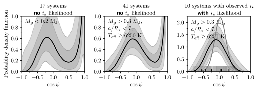
Figure 33: Hierarchical Bayesian inference of the obliquity distribution for subsets of the sample that are suspected of being especially prone to misalignment. The left panel is for all sub-Saturns with $\lambda$ measurements, without using any $i_{\star}$ information even when it is available. The middle panel is for all hot Jupiters around hot stars with $\lambda$ measurements, without using any $i_{\star}$ information even when it is available. The right panel is for hot Jupiters around hot stars for which both $\lambda$ and $i_{\star}$ are known and utilized. In the right panel, the black upward tick marks on the horizontal axis are the individual values of $\cos\psi$, and the horizontal bands surrounding the tick marks convey the uncertainties. The solid gray curve is a KDE estimated from these measurements.

Although the results are too prior-dependent to be sure, these results lead us to hypothesize that the preponderance of polar planets is a phenomenon specific to hot Jupiters around hot stars and possibly also sub-Saturns. The hot stars, in particular, are more amenable to the determination of $i_{\star}$ via the $v\sin i$ method, given their higher rotation velocities, possibly explaining their over-representation in the $\lambda$ & $i_{\star}$ sample.

If there truly is a preponderance of systems with nearly polar orbits, it would seem to be a clue about the history of these systems. For example, for the sub-Saturn population, Petrovich et al. (2020) proposed that nearly polar orbits of Neptune-mass planets can result from a secular resonance between the nodal precession frequencies induced by the protoplanetary disk and by an outer companion. One might test this theory by searching for distant massive companions to the polar-orbiting planets. In any case, Petrovich et al. (2020) note that their theory is not applicable to hot Jupiters.

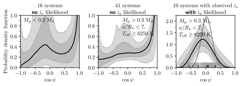
Figure 34: Hierarchical Bayesian inference of the obliquity distribution for the same subsets as in Fig. 33, but here a uniform prior, $\mathcal{U}(-4,10)$, was applied to $\log\kappa$ in the “DFM” code.

Tidal evolution might lead to a pile-up of polar orbits of hot Jupiters around hot stars. Lai (2012) demonstrated that orbital orientations can linger near $90^{\circ}$ when damping is from the dissipation of inertial waves in the convective envelope of a star. In general, this theory requires the planet’s orbital angular momentum to be larger than the star’s spin angular momentum to avoid producing more systems near 180^∘ than are observed (e.g. Li & Winn, 2016).

5.2 Obliquity – Eccentricity correlation?

Explaining the existence of giant planets on orbits well within the “ice line” of the protoplanetary disk is one of the oldest unsolved problems in exoplanetary science. Disk-driven migration is one possibility, and would generically yield low eccentricities and obliquities (e.g., Lin et al., 1996; Dawson & Johnson, 2018). In this scenario, the observed cases of high eccentricity and obliquity arise from other processes. An alternative idea is to combine eccentricity-raising dynamical interactions – such as planet-planet scattering or Kozai-Lidov cycles – and tidal dissipation (e.g., Fabrycky & Tremaine, 2007; Chatterjee et al., 2008; Nagasawa et al., 2008). If the eccentricity reaches a high enough value, or more to the point, if the periastron distance reaches a low enough value, the damping of tidal oscillations in either the planet or star can convert orbital energy into heat and thereby shrink the semi-major axis.

In many of the proposed scenarios for raising of the eccentricity, the orbital inclination relative to the initial plane is also increased, which could lead to a high stellar obliquity. Therefore, if the dynamical scenarios are correct, one might expect to see a correlation between $e$ and $\lambda$ for the affected planets. An important caveat is that tidal damping tends to reduce both the eccentricity and stellar obliquity, but on timescales that might differ by orders of magnitude. This is not only because eccentricity and obliquity tides excite different types of perturbations, but also because eccentricity damping can take place inside either body while significant obliquity damping requires the energy to be dissipated inside the star (Ogilvie, 2014). Thus, tides might confound the interpretation of any correlation. For example, if eccentricity damping is much faster than obliquity damping, then any initial correlation might be diminished on astronomically short timescales. Or, tidal dissipation might increase the correlation by boosting the number of low-$e$, low-$\lambda$ systems even if there were little or no correlation before tidal evolution.

Regarding the latter point, $a/R_{\star}$ and $\lambda$ are known to be positively correlated for cool stars (Albrecht et al., 2022). This has been interpreted as evidence for tidal dissipation, since dissipation rates should decline sharply with $a/R_{\star}$. Furthermore, $a/R_{\star}$ is known to be positively correlated with $e$, presumably for the same reason (although the causal variable might be $a/R_{\rm p}$ in that case). Taken together, these two correlations might cause $e$ and $\lambda$ to be correlated without invoking any new explanation.

Nevertheless, it is well worth testing for a correlation between $e$ and $\lambda$ in the current sample and Rice et al. (2022a) investigated both of these parameters. Specifically they found at the Kraft break, the cumulative sum of $\lambda$ for systems with eccentric orbits differs by $6.5\sigma$ from the $\lambda$ distribution of systems with circular orbits. For systems with giant-planet they obtain an $8.7\sigma$ result. Their procedure was as follows, as we understand it. They selected systems with periastron distances $\leq 0.1$ AU for which a value of $\lambda$ was reported in the TEPCat obliquities table, looked up $e$ in the NASA Exoplanet Archive (NEA) Confirmed Planets list, and separated the systems into two samples: an eccentric sample ($e\geq 0.1$), and a circular sample ($e=0$). They omitted borderline systems with $0<e<0.1$. They arranged the planets in order of the star’s effective temperature, giving each planet a position $i$ in a line of $N$ planets. They examined the cumulative sums of $|\lambda|$ for the eccentric sample, with the $j$th cumulative sum defined as the sum of all $|\lambda_{i}|$ values for $i\leq j$. Since the eccentric sample contained fewer systems and had a different distribution of stellar types than the circular sample, Rice et al. (2022a) used a Monte Carlo procedure to make “matching” eccentric samples for comparison. They created 5000 matching circular samples by drawing randomly (with replacement) from the circular sample the same number of stars with $T_{\rm eff}<6100$ K and the same number of stars with $T_{\rm eff}>6100$ K as in the eccentric sample. They then compared the $N$th cumulative sums of the eccentric sample and the ensemble of matching circular samples, and found them to differ by $6.5\sigma$, where $\sigma$ was determined from the spread amongst the 5000 trials. For convenience we will denote the “number-of-sigma” by the symbol $\Delta$.

They also tried some variations on the samples. When performing the same steps but with the samples restricted to giant planets, defined as $M_{\rm p}>0.3$ M_J, they found $\Delta=8.7$. To test the notion that $a/R_{\star}$ is a “hidden variable” responsible for the $e/\lambda$ correlation, they created samples that were not divided by eccentricity, but rather on whether $a/R_{\star}$ is greater or smaller than 12. In this case, they found $\Delta=4.9$, and since this is smaller than 6.5 they concluded that the variation in $a/R_{\star}$ cannot explain the entire effect they observed between $e$ and $\lambda$.

With the enlarged sample, we decided to revisit these intriguing results. After implementing the method of Rice et al. (2022a) to the best of our ability, we found $\sigma=2.1$ for the whole sample shown in Fig. 35 and $\sigma=4.1$ for planets with $M_{\rm p}>0.3$ M_J. To check on our code, we tried reproducing their results using the systems known at that time and were unsuccessful. Further investigation showed that the main reason for the discrepancy can be traced to 6 systems in the eccentric sample that should have been in the circular sample. These 6 systems (with details in the footnotes) are HAT-P-23 b and HAT-P-32 b KELT-6 b.; and HATS-14 b, HATS-70 b, & Kepler-63 b Taken together, these errors caused $\sigma$ to appear larger than in reality.

We tried some variations on the samples. When including systems with $0<e<0.1$ in the circular group, instead of omitting them, we found $\Delta=1.8$. When focusing on giant planets ($M_{\rm p}>0.3$ M_J), we obtained $\Delta=4.6$. We note that there are only 10 known eccentric giant planets around cool stars, making the results sensitive to an error for an individual system. When we tried dividing the sample according to whether $a/R_{\star}$ is smaller or greater than 12, instead of by eccentricity, we found $\Delta=8.1$ as shown in Fig. 36. Thus, in our case, the $\sigma$ statistic is larger when testing the effect of $a/R_{\star}$ than when testing for the effect of eccentricity.

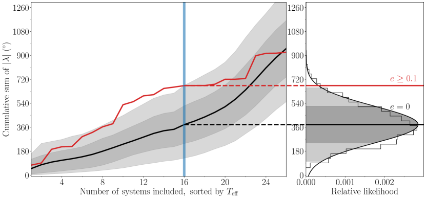
Figure 35: Obliquity distribution for stars hosting planets on eccentric and circular orbits. Left: The cumulative sum of $|\lambda|$ for eccentric planets shown in red, sorted by $T_{\rm eff}$. The black line is the average of 5000 randomly sampled sets from the circular population with the gray shaded area denoting the 1$\sigma$ and 2$\sigma$ intervals. The vertical blue line denotes the Kraft break ($T_{\rm eff}=6100$ K). Right: Histogram showing the distribution of the circular population and the value of the eccentric population at the Kraft break. The Gaussian is a fit to the histogram. The circular and eccentric samples only differ by $2.1\sigma$, meaning the eccentric population does not appear to be significantly more misaligned. Adapted from Rice et al. (2022a).

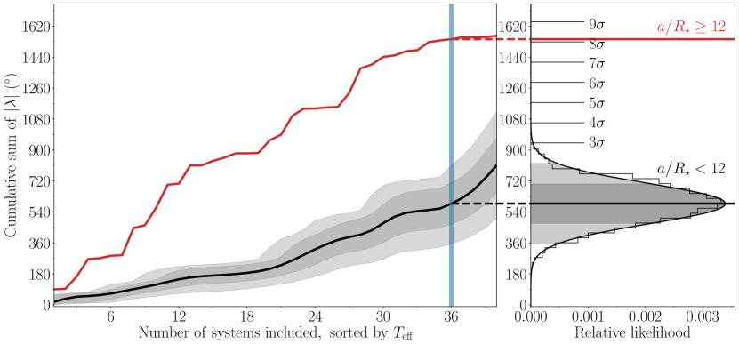
Figure 36: Obliquity distribution for stars hosting planets on close-in and wide orbits. Same as Fig. 35, but for systems with planets on close-in or wide orbits with the division given for $a/R_{\star}=12$. The systems with planets on wider orbits appear to be significantly more misaligned compared to those with planets closer in.

5.3 Tidal realignment

The main evidence that tidal obliquity damping occurs on astrophysically relevant timescales, despite many researchers’ early expectations (see, e.g., Queloz et al., 2000; Winn et al., 2005), is that the types of systems where one might expect tidal dissipation rates to be fastest — with massive, close-orbiting planets and host stars with thick convective envelopes — do indeed have an obliquity distribution that is concentrated around $0^{\circ}$. And conversely, systems for which misalignment is proposed to be part of the formation process but for which tidal dissipation rates are expected to be much slower — somewhat wider-orbiting giant planets, and stars with radiative envelopes — have a broad obliquity distribution. For some details on these findings, see Schlaufman (2010); Winn et al. (2010a), and Hébrard et al. (2011). To demonstrate this point more explicitly, Albrecht et al. (2012b) constructed a crude “tidal dissipation figure of merit” for each system, meant to be a proxy for the tidal dissipation rate, and showed that the obliquity distribution does indeed narrow for the systems where the figure of merit predicts more rapid dissipation.

However, the precise mechanisms of tidal dissipation are not well understood and are probably quite complex, depending on forcing frequency, stellar structure, rotation rate, etc. Another problem with tidal damping is that the expected endpoint of tidal evolution for most of the known close-orbiting giant planets is tidal orbital decay and destruction (Brown et al., 2011). Thus, an observed planet around a star that experienced tidal damping must somehow have avoided orbital decay before the star was aligned to the observed degree.

Several theories exist that might prevent or at least delay planet destruction for long enough to be consistent with the data. The orbital angular momentum of some lucky planets may exceed the host’s spin angular momentum, causing the star to align before its orbital decays (see, e.g., Hansen, 2012; Valsecchi & Rasio, 2014; Dawson, 2014). If tidal damping is primarily driven by the dissipation of inertial waves in a star’s convective zone, then alignment could be faster than orbital decay (Lai, 2012; Lin & Ogilvie, 2017; Damiani & Mathis, 2018). The damping of gravity waves in radiative cores might similarly cause alignment before tidal in-spiral (Zanazzi et al., 2024). Another idea is that if the efficiency of tidal dissipation drops sharply with increasing forcing frequency (shorter orbital periods), then alignment can be arranged to occur before tidal evolution slows down dramatically, allowing the orbit to survive (Barker & Ogilvie, 2010; Penev et al., 2018; Anderson et al., 2021; Ma & Fuller, 2021). Alternatively, and more speculatively, tides from the planet might only affect a star’s outer convective zone, allowing the planet to donate a smaller amount of its orbital angular momentum to spin up the star and save itself (Winn et al., 2010a). With all of this theoretical uncertainty, is there a relatively model-independent way to seek corroborating evidence for tidal obliquity damping?

The Sun’s obliquity is $7.155^{\circ}$ relative to the ecliptic (Beck & Giles, 2005) and $6.2^{\circ}$ relative to the Solar System’s invariable plane (see, e.g., Souami & Souchay, 2012; Gomes et al., 2017). If we assume this angle to be representative of the degree to which stars and their planetary systems are initially aligned — admittedly, a big assumption — then we would expect some systems that have experienced strong tidal damping to have obliquities much smaller than 6^∘. This can be tested with high-precision RM observations of the types of systems where strong tidal damping is expected, and comparisons to systems where it is not expected.

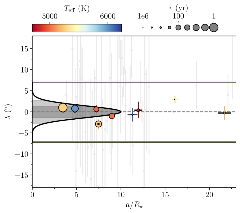
Figure 37: Precise projected obliquity measurements. Here we highlight the most precise ($\sigma_{\lambda}\leq 2^{\circ}$) measurements of $\lambda$ for systems with cool stellar hosts ($T_{\rm eff}<6100$ K). WASP-50 is highlighted with a black center. The color-coding is done according to $T_{\mathrm{eff}}$ and the marker sizes scale with the tidal alignment timescale (as given by Zahn, 1977). The gray shaded area shows the Gaussian distribution inferred from cool hosts ($T_{\rm eff}<6100$ K) with close-in ($a/R_{\star}<10$), massive ($M_{\rm p}<0.3$ M_J) planets. The horizontal lines demarcate the Solar System obliquity of $7.155^{\circ}$ (Beck & Giles, 2005). The light gray error bars show the less precise measurements. Adapted from Albrecht et al. (2022, Figure 10).

Focusing on only the most precise measurements ($\sigma_{\lambda}<2^{\circ}$) in cool hot Jupiter systems, Albrecht et al. (2022, Section 3.1.8) found the dispersion of $\lambda$ measurements to be $0.91^{\circ}$. Given an average measurement uncertainty of $0.82^{\circ}$, this should probably be regarded as an upper limit on the true dispersion of a few degrees. There are drawbacks to this simple approach. First, one must decide what constitutes a “precise” measurement. Somewhat arbitrarily, Albrecht et al. (2022) chose a threshold precision of $2^{\circ}$. Second, it ignores the information contained in the much more numerous and less precise measurements.

We tried overcoming these problems with a Hierarchical Bayesian Model (HBM), following up on the work by Siegel et al. (2023), who carried out similar tests to those described below. (To eliminate any suspense, we obtained similar results, too.) The hyper-parameter of interest is the dispersion of the underlying $\lambda$ distribution around $0^{\circ}$, independent of measurement uncertainties. To identify systems for which rapid tidal dissipation is expected, we required $T_{\rm eff}<6100$ K, $a/R_{\star}<10$, and $M_{\rm p}>0.3$ M_J. We also required $\sigma_{\lambda}<50^{\circ}$. This led to a sample of 60 systems, only one of which stood out: TOI-858Bb (Hagelberg et al., 2023a), which is located in a wide binary system and has a retrograde orbit. Since tidal dissipation is evidently not the only important obliquity-altering process in this system — perhaps due to the stellar companion — we decided to omit it from consideration, leaving a sample of 59 systems. Fig. 37 shows the key characteristics of those 59 systems (as well as some systems with higher values of $a/R_{\star}$). The data points with a precision in $\lambda$ better than $2^{\circ}$ are highlighted; the measurement of WASP-50 of $-2.9\pm 1.2$^∘ presented in this paper is included in this sample.

The result of the HBM was a dispersion in $\lambda$ of $1.4\pm 0.7^{\circ}$, depicted in Fig. 37 as a Gaussian function with a width of $1.4^{\circ}$. For prograde systems the expected endpoint of the alignment process is $\lambda=0^{\circ}$, which is why our HBM did not include a hyperparameter for the mean of the obliquity distribution. However, as an experiment to check for surprises or systematic errors (such as the neglect of the convective blueshift) we repeated the analysis after allowing for the mean to be a second hyperparameter. The results were a a dispersion of $1.5\pm 0.8^{\circ}$ and a mean of $-0.2\pm 0.7^{\circ}$, giving no clear evidence for surprises or systematic errors.

In the light of these results, our measurement of WASP-50 ($-2.9\pm 1.2$^∘) is more interesting than we originally anticipated. According to the rough criteria described above, the tidal dissipation timescale for this system should be faster than in most of the other systems in the sample. Gillon et al. (2011) reported an age of $7.0\pm 3.5$ Gyr based on comparing the usual photometric and spectroscopic observables to stellar-evolutionary models. However, the estimated age based on the chromospheric activity and rotational period was only $0.8\pm 0.4$ Gyr (which could also be a result of tidal spin-up, e.g., Tejada Arevalo et al., 2021). If the old age is correct, the system is more likely to have had enough time to achieve good alignment than if the young age is correct. As discussed in Section 3.2.2, Gillon et al. (2011) reported a rotation period for WASP-50 of $16.3\pm 0.5$ d or potentially twice this value. Using these values $\psi$ comes out to $34^{+12}_{-9}$ and $5.0^{+1.9}_{-3.0}$, respectively. The value of the rotation period has dramatic consequences for the inferred orientation of the system; the shorter period we identified in the TESS light curve results implies an even more misaligned system, which seems worth checking on, given that so many other similar systems are well-aligned. Future TESS observations might be able to resolve the issue.

Considering planets on wider orbits, with $10\leq a/R_{\star}<20$, the HBM yielded a dispersion of $8\pm 2^{\circ}$. The spread in $\lambda$ is therefore seen to increase with orbital separation (as also discussed in Section 5.2). When restricted to planets with $20\leq a/R_{\star}<30$ (a sample of only 7 systems), the HBM yielded a dispersion of $4\pm 3^{\circ}$, which is consistent with the $10\leq a/R_{\star}<20$ results. It would be interesting to obtain more measurements for planets with large separations to bolster these results and possibly even investigate the separation-dependence of tidal dissipation rates.

5.4 Compact multi-transiting systems, with and without outer companions

At a time when only five $\lambda$ measurements had been made for stars with more than one known transiting planets, Albrecht et al. (2013) noted that they were all consistent with good alignment. The number is now 22, including four systems we have added to the tally in this work. For WASP-148, $\lambda$ had already been measured by Wang et al. (2022), and our result is consistent with theirs but with lower precision. For TOI-1130, we found $\lambda=$ $4^{+5}_{-6}$^∘, while for two other systems, LTT 1445A and TOI-451A, our formal results were that the orbits are prograde, but given the low SNR of our measurements we do not include them in the following discussion. We do include an additional 4 systems for which there are good constraints on the stellar inclination even though $\lambda$ is not known. Our discussion is therefore based on the properties of 24 systems.

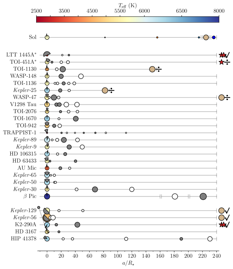
Figure 38: Obliquities of stars with multiple transiting planets, as constrained by either the RM effect or asteroseismology. Each horizontal line shows the $a/R_{\star}$ values of the planets in a given system, with the solar system on top (with gaps to allow Jupiter and Neptune to be shown). For the planets, the size of each circle conveys the planet’s radius relative to Jupiter. For the stars, symbol size conveys the radius relative to the Sun, with a color conveying the effective temperature. Gray circles are planets for which the RM effect has been measured – except for $\beta$ Pic b where spectro-interferometry was used. The wedge indicates the projected obliquity for a given system, based on the most precise measurement for any planet in the system, with the exception of HD 3167 for which two planets appear to have very different inclinations. The asteroseismic measurements constrain $i_{\star}$ and not $\lambda$; in those cases the wedge should therefore be read as aligned (Kepler-50 and Kepler-65) or misaligned (Kepler-56, Kepler-129). Planetary (tan circle) or stellar companions (red star, M-dwarfs) to a given system are shown to the right, where $\surd$ ($\div$) denotes that the companion could (not) have influenced the obliquity of the inner planetary system. The asterisks for LTT 1445A and TOI-451A denote that these measurements should be taken with a grain of salt. Adapted from Wang et al. (2022, Figure 3).

Fig. 38 is a family portrait of these systems. The Solar System is shown at the top for scale and reference. There are 19 systems for which the data are consistent with zero obliquity. There are 5 systems with large obliquities relative to at least one transiting planet: HD 3167, Kepler-56, HIP 41378, Kepler-129, and K2-290. HD 3167 has a very unusual architecture in which the planets appear to be on perpendicular orbits (Bourrier et al., 2021a). This case is illustrated in Fig. 38 as the outer planet floating over Kepler-129. HIP 41378 is a five-planet system in which Grouffal et al. (2022a) measured the projected obliquity with respect to planet d to be $57^{+26\circ}_{-18}$. However, due to the long duration ($\sim 12.5$ hr and $P\sim 278$ d), a full transit was not observed, preventing us from having high confidence in the result.

In Fig. 38 Kepler-30 is grouped with the aligned systems, but there are conflicting indications about the obliquity. By using two different methods Sanchis-Ojeda et al. (2012) found $\lambda=-1\pm 10^{\circ}$ and $\lambda=4\pm 10^{\circ}$, indicating a well-aligned system. However, Morgan et al. (2023) found $i_{\star}=43^{+15\circ}_{-9}$, indicating a large misalignment, based on the combination of the rotation period, $v\sin i_{\star}$, and $R_{\star}$. However, this result depends critically on the value $v\sin i_{\star}$ $=2.0\pm 0.2$ km/s reported by Fabrycky et al. (2012), and the measurement uncertainty of 0.2 km/s is likely to have been underestimated. Systematic errors of at least 0.5 km/s are typical, due to effects such as turbulent and instrumental broadening. A value of $3.0\pm 0.5$ km s^-1 would allow for consistency with alignment ($i_{\star}\approx 90^{\circ}$).

In contrast to hot Jupiter systems, where misalignments might have occurred in the tumultuous process of high-eccentricity migration after disk dispersal, the misalignments in multiplanet systems might have occurred while the disk was present. Gravitational interactions between a planet-forming disk, a binary companion, and a spinning host star can be enhanced when the disk looses mass, magnifying the host star’s tilt through a secular resonance (e.g. Batygin & Adams, 2013). For a binary companion to generate spin-orbit misalignments, the stellar spin must be gravitationally decoupled from the planet forming in the disk, otherwise the star’s spin axis and planet’s orbit normal precess in-unison (eq. 80 of Zanazzi & Lai 2018). The spin is decoupled from the orbits of LTT 1445Ab, and K2-290Ab,c, but not for TOI-451Ab, when torqued by their binary companions.

Similarly, sweeping secular resonances from a dispersing disk can enhance gravitational interactions between forming planets, magnifying their inclinations (e.g. Ward, 1981). However, for planetary companions to generate misalignments, they must also supply the system with a large angular momentum deficit to misalign an inner planet. Based on the work by Petrovich et al. (2020); Zanazzi & Chiang (2024), we assume a planetary companion (mass $m_{2}$, semi-major axis $a_{2}$) could secularly misalign an inner planet (mass $m_{1}$, semi-major axis $a_{1}$) if they are well separated ($a_{2}/a_{1}>2$), and they have a large angular momenta ratio ($(m_{2}a_{2}^{1/2})/(m_{1}a_{1}^{1/2})>10$, see e.g. eq. 22 of Zanazzi & Chiang 2024). The planet pairs Kepler-56 c,d and Kepler-129 c,d meet this criteria, while Kepler-25 c,d, WASP 47 b,c, and TOI-1130 c,d do not, although we note that the companion TOI-1130 d is as of yet poorly constrained (Korth et al., 2023). LTT 144A might be aligned when a misalignment is predicted by Zanazzi & Lai (2018), while the other systems with distant, massive companions appear consistent with spin-orbit misalignments being generated (or not) while gas disk is present (Fig. 38).

Secular interactions from companions exciting an inner planet’s inclination during the disk-hosting phase is not the only mechanism which can explain misalignments in multiplanet systems. For instance, Gratia & Fabrycky (2017) postulate a dynamical instability between three outer planets could have misaligned Kepler-56 b and c, while Best & Petrovich (2022) find secular chaos induced by the two binary companions of K2-290A is sufficient to misalign K2-290Ab and c, with both mechanisms taking place after disk dispersal. Additional stellar obliquity measurements in multiplanet systems with companions (e.g. LTT 1445A), and further constraints on the presence or absence of companions in inclined multiplanet systems (e.g. HD 3167, HIP 41378), could constrain which mechanisms are responsible for generating misalignments.

For the multiplanet systems which have obliquities consistent with alignment (again barring TOI-451A and LTT 1445A), we applied the HBM framework described in the previous section to infer the mean $\mu$ and dispersion $\sigma$ of the intrinsic distribution of obliquities. The results were $\mu=0.0\pm 1.7^{\circ}$ and $\sigma=2.0\pm 1.5^{\circ}$. When we removed Kepler-30 c from the sample, out of the concern raised above, we found $\mu=0.0\pm 1.8^{\circ}$ and $\sigma=2.1\pm 1.6^{\circ}$. Thus, the obliquity dispersion of the host stars of multis is similar to that of cool stars with hot Jupiters. However, tidal obliquity damping is expected to be much weaker for the multis than for the hot Jupiters, because of the planets’ lower masses and relatively wider orbits. The low obliquities of the multis might therefore be primordial, i.e., due to the flatness of the protoplanetary disk and its strong coupling to the accreting young star. From this point of view, the solar obliquity of 6^∘ may be unusually high — and if the high solar obliquity is simply a peculiarity of the Solar System, then the evidence for tidal obliquity damping presented in the previous section would be undermined.

We finally note that an additional aligned system could potentially be the HD 148193 system ($\lambda=$ $14^{+7}_{-8}$^∘, Section 4.2), if the inner transiting candidate is confirmed as a bona fide planet at some point.

6 Conclusions

We presented new observations of the RM effect for 19 stars with transiting planets. We combined these measurements with results from the literature to arrive at a sample of 205 systems for which $\lambda$ has been determined with reasonable confidence. With this sample, we revisited four questions:

1. Is there a preponderance of perpendicular planets? First raised as a possibility by Albrecht et al. (2021), and then questioned Siegel et al. (2023) and Dong & Foreman-Mackey (2023), our updated sample does not settle the matter. It remains the case that a “polar peak” is seen in the obliquity distribution of the sample of planets for which $\lambda$ and $i_{\star}$ have been measured, but no such peak is seen clearly when analyzing the larger sample of systems for which $\lambda$ has been measured but not necessarily $i_{\star}$. We showed that the two samples might differ from each other because certain kinds of systems — namely, hot stars with hot Jupiters — are more amenable to $i_{\star}$ measurements than others and also more likely to have near-polar orbits. The subsample of sub-Saturns around cooler stars also seems to have a preference for polar orbits, although the sample needs to be increased to be sure. Thus, the resolution of this issue still seems likely to be astrophysically interesting.

2. Is there a correlation between orbital eccentricity and stellar obliquity for close-orbiting giant planets? We concluded that the correlation is weaker than had been previously reported by Rice et al. (2022a). Furthermore, we argued that the correlation exists because both eccentricity and obliquity are correlated with a third variable, orbital separation. The causal mechanism is likely to be tidal dissipation, which lowers both eccentricity and obliquity at short orbital separations.

3. How low are the obliquities of stars suspected of having been subject to tidal obliquity damping? Measurements of $\lambda$ of cool stars with close-orbiting giant planets ($T_{\rm eff}<6100$ K, $a/R_{\star}<10$, $M_{\rm p}>0.3$ M_J) have an intrinsic dispersion of $1.4\pm 0.7^{\circ}$ in $\lambda$, according to our Hierarchical Bayesian Model (HBM). Such fine alignment can be considered as supporting evidence for tidal obliquity damping, if the solar obliquity of 6^∘ is taken as representative of a typical un-damped “primordial” obliquity. More precise measurements of $\lambda$ in systems hosting massive planets around cool stars might even help to quantify the dependence of tidal dissipation rates on orbital separation.

4. How well aligned are the central stars of compact systems of multiple transiting planets? Except for a few notable exceptions, the $\lambda$ measurements in compact multiplanet systems are consistent with low obliquities. For this sample, we found an intrinsic dispersion in $\lambda$ of $2.1\pm 1.6^{\circ}$. In this sense, the multis are better aligned than the Solar System, indicating that compact multis are born unusually flat or that the Sun is unusually tilted, complicating the conclusions drawn above about tidal obliquity damping. The few examples of misaligned stars with compact systems of multiple transiting planets might be explained by interactions between the protoplanetary disk and a stellar companion, or by interactions with outer giant planets after the epoch of planet formation.

Appendix A Additional figures

Appendix B Additional tables

Table 9: MCMC posteriors.

	$a/R_{\star}$	$R_{p}/R_{\star}$	$\cos i$	$K$	$\gamma$	$\sigma$
				(m s-1)	(m s-1)	(m s-1)
HD 118203 b	$7.23^{+0.16}_{-0.18}$	$0.0546^{+0.0005}_{-0.0004}$	$0.027^{+0.010}_{-0.026}$	$196^{+17}_{-19}$	$-28881^{+6}_{-7}$	$11^{+2}_{-3}$
HD 148193	$23.1^{+1.7}_{-0.8}$	$0.0455^{+0.0006}_{-0.0005}$	$0.016_{-0.007}^{+0.008}$	$42^{+21}_{-33}$	$-50340.6^{+1.3}_{-1.2}$	$1.2^{+0.5}_{-0.5}$
K2-261 b	$14\pm 2$	$0.0524^{+0.0005}_{-0.0006}$	$0.025^{+0.011}_{-0.025}$	$18^{+8}_{-11}$	$3338^{+2}_{-3}$	$0.8^{+0.3}_{-0.8}$
K2-287 b	$25.4^{+1.1}_{-1.2}$	$0.0783\pm 0.0007$	$0.026\pm 0.004$	$52^{+13}_{-12}$	$32872\pm 6$	$1.3^{+0.3}_{-0.4}$
KELT-3 b	$5.64^{+0.05}_{-0.06}$	$0.0932\pm 0.0002$	$0.120\pm 0.003$	$282\pm 13$	$28333\pm 2$	…
KELT-4Ab	$6.02^{+0.09}_{-0.10}$	$0.1011^{+0.0006}_{-0.0009}$	$0.110^{+0.005}_{-0.004}$	$53^{+28}_{-23}$	$-23145^{+5}_{-4}$	$8^{+3}_{-7}$
LTT 1445Ab	$29.9^{+1.5}_{-1.3}$	$0.0487^{+0.0017}_{-0.0018}$	$0.009^{+0.004}_{-0.009}$	$-4^{+7}_{-16}$	$-4088^{+8}_{-10}$	$6.7^{+1.4}_{-2.1}$
TOI-451Ab	$6.2^{+0.8}_{-0.6}$	$0.0203^{+0.0010}_{-0.0011}$	$0.06^{+0.03}_{-0.06}$	$5^{+3}_{-4}$	$19755.7\pm 0.8$	$1.9\pm 0.7$
TOI-813 b	$47^{+4}_{-2}$	$0.0324\pm 0.0007$	$0.008^{+0.004}_{-0.005}$	$95^{+51}_{-95}$	$1199.6^{+1.7}_{-1.3}$	$0.5^{+0.2}_{-0.5}$
TOI-892 b	$15.1^{+0.4}_{-0.3}$	$0.0790^{+0.0007}_{-0.0008}$	$0.021^{+0.005}_{-0.006}$	$54^{+23}_{-54}$	$41907^{+30}_{-49}$	…
TOI-1130 b	$22.1\pm 0.4$	$0.176^{+0.013}_{-0.021}$	$0.0432^{+0.0016}_{-0.0024}$	$152\pm 15$	$-8033.6\pm 1.6$	$1.6\pm 0.8$
WASP-50 b	$7.47^{+0.08}_{-0.09}$	$0.1371\pm 0.0006$	$0.093\pm 0.002$	$253.5^{+1.5}_{-1.4}$	$25421.1\pm 0.3$	$0.6^{+0.3}_{-0.5}$
WASP-59 b	$25.4^{+1.1}_{-1.0}$	$0.136\pm 0.002$	$0.019^{+0.003}_{-0.004}$	$186^{+20}_{-19}$	$-0.6^{+1.1}_{-1.0}$	$2.7\pm 0.9$
WASP-136 b	$7.4\pm 0.2$	$0.0672\pm 0.0005$	$0.041^{+0.016}_{-0.013}$	$146^{+52}_{-59}$	$-3^{+7}_{-8}$	$12^{+7}_{-9}$
WASP-148 b	$14.4\pm 0.3$	$0.09082\pm 0.00020$	…	$11^{+6}_{-11}$	$-5507\pm 3$	$1.6^{+0.8}_{-1.6}$
WASP-172 b	$7.58\pm 0.17$	$0.0893\pm 0.0005$	$0.061^{+0.007}_{-0.006}$	$53^{+25}_{-43}$	$-20410\pm 5$	$11\pm 3$
WASP-173Ab	$5.12^{+0.03}_{-0.02}$	$0.1176\pm 0.0006$	$0.012^{+0.006}_{-0.012}$	$625^{+5}_{-4}$	$-7922\pm 3$	$9.6^{+1.5}_{-1.8}$
WASP-186 b	$9.9\pm 0.3$	$0.0812^{+0.0007}_{-0.0006}$	$0.090\pm 0.005$	$529^{+132}_{-154}$	$-240^{+43}_{-42}$	$16^{+7}_{-16}$
XO-7 b	$6.54^{+0.07}_{-0.06}$	$0.0923\pm 0.0003$	$0.107\pm 0.002$	$128^{+48}_{-59}$	$-13050^{+10}_{-11}$	$7^{+4}_{-5}$
WASP-26 b	$6.7\pm 0.3$	$0.097^{+0.013}_{-0.009}$	$0.122^{+0.009}_{-0.008}$	$142\pm 15$	$-16\pm 3$	$10.2^{+1.5}_{-1.7}$

• For WASP-148 b we were stepping in $i$, where we got $i=86.57_{-0.16}^{+0.16\circ}$.

Values for the new literature systems are drawn from the following references (with bold denoting the source for $\lambda$): 55 Cnc e: 1 Rosenthal et al. (2021), 2 Zhao et al. (2023). CoRoT-36 b: 1 Sebastian et al. (2022). HAT-P-11 b: 1 Sanchis-Ojeda & Winn (2011), 2 Winn et al. (2010b). HAT-P-3 b: 1 Bonomo et al. (2017b) , 2 Bourrier et al. (2023), 3 Mancini et al. (2018). HAT-P-30 b: 1 Bonomo et al. (2017b), 2 Cegla et al. (2023). HAT-P-32 b: 1 Bonomo et al. (2017b), 2 Czesla et al. (2023), 3 Albrecht et al. (2012c). HAT-P-33b: 1 Wang et al. (2017), 2 Bourrier et al. (2023). HAT-P-49 b: 1 Bieryla et al. (2014), 2 Bourrier et al. (2023). HD 3167 c: 1 Bourrier et al. (2021b). HD 106315 c: 1 Zhou et al. (2018), 2 Bourrier et al. (2023). HD 189733 b: 1 Bonomo et al. (2017b), 2 Cristo et al. (2024). HIP 41378 d: 1 Lund et al. (2019), 2 Santerne et al. (2019), 3 Grouffal et al. (2022b). K2-29 b: 1 Santerne et al. (2016). K2-105 b: 1 Narita et al. (2017), 2 Castro-González et al. (2022), 3 Bourrier et al. (2023). KELT-10 b: 1 Kuhn et al. (2016), 2 Steiner et al. (2023). KELT-11 b: 1 Beatty et al. (2017), 2 Mounzer et al. (2022). KELT-19 b: 1 Kawai et al. (2024), 2 Siverd et al. (2018). Kepler-63 b: 1 Sanchis-Ojeda et al. (2013b). MASCARA-2 b: 1 Singh et al. (2023). MASCARA-4 b: 1 Ahlers et al. (2020), 2 Dorval et al. (2020). Qatar-6 b: 1 Rice et al. (2023a). TOI-640 b: 1 Knudstrup et al. (2023b). TOI-677 b: 1 Sedaghati et al. (2023). TOI-1670 c: 1 Lubin et al. (2023). TOI-858Bb: 1 Hagelberg et al. (2023b). TOI-1136 d: 1 Dai et al. (2023). TOI-1478 b: 1 Rodriguez et al. (2021), 2 Rice et al. (2022b). TOI-1842 b: 1 Hixenbaugh et al. (2023). TOI-1937 b: 1 Yee et al. (2023). TOI-2025 b: 1 Knudstrup et al. (2022). TOI-2076 b: 1 Osborn et al. (2022), 2 Frazier et al. (2023). TOI-2202 b: 1 Rice et al. (2023b). TOI-3884 b: 1 Libby-Roberts et al. (2023). WASP-7 b: 1 Bonomo et al. (2017b), 2 Albrecht et al. (2012a). WASP-12 b: 1 Bonomo et al. (2017b), 2 Albrecht et al. (2012c). WASP-33 b: 1 Johnson et al. (2015). WASP-47 b: 1 Bourrier et al. (2023), 2 Sanchis-Ojeda et al. (2015). WASP-52 b: 1 Bonomo et al. (2017b), 2 Cegla et al. (2023). WASP-62 b: 1 Garhart et al. (2020), 2 Brown et al. (2017). WASP-76 b: 1 Ehrenreich et al. (2020). WASP-85 b: 1 Močnik et al. (2016). WASP-94Ab: 1 Neveu-VanMalle et al. (2014). WASP-106 b: 1 Wright et al. (2023). WASP-107 b: 1 Piaulet et al. (2021), 2 Bourrier et al. (2023). WASP-121 b: 1 Bourrier et al. (2020). WASP-131 b: 1 Doyle et al. (2023). WASP-156 b: 1 Demangeon et al. (2018), 2 Saha et al. (2021), 3 Bourrier et al. (2023). WASP-166 b: 1 Bourrier et al. (2023). WASP-167 b: 1 Temple et al. (2017). XO-6 b: 1 Crouzet et al. (2017).

Table 10: Extension to Table A1 of Albrecht et al. (2022).

Planet	$a/R_{\star}$	$M_{\rm p}$	$R_{\rm p}$	$e$	$\lambda$	$i_{\star}$	$\psi$
		(MJ)	(RJ)		(∘)	(∘)	(∘)
55 Cnc e	$3.52\pm 0.04$	$0.0251\pm 0.0010$	$0.165\pm 0.002$	$0.04\pm 0.03$	$10^{+17}_{-20}$	$75^{+11}_{-17}$	$23^{+15}_{-23}$
CoRoT-36 b	$9.3\pm 1.0$	$<0.7$	$1.41\pm 0.14$	…	$276\pm 11$	…	…
HAT-P-11 b	$16.6\pm 0.3$	$0.087\pm 0.010$	$0.389\pm 0.005$	$0.2644\pm 0.0006$	$103^{+26}_{-10}$	$67^{+2}_{-4}$	$97^{+8}_{-4}$
HAT-P-3 b	$9.8\pm 0.3$	$0.59\pm 0.02$	$0.91\pm 0.03$	$0.000\pm 0.010$	$21\pm 9$	$16^{+6}_{-7}$	$76\pm 8$
HAT-P-30 b	$7.4\pm 0.3$	$0.71\pm 0.03$	$1.34\pm 0.07$	$0.000\pm 0.016$	$70\pm 3$	…	…
HAT-P-32 b	$6.05\pm 0.12$	$0.80\pm 0.14$	$1.81\pm 0.03$	$0.00\pm 0.04$	$85.0\pm 1.5$	…	$84.9\pm 1.5$
HAT-P-33 b	$5.7\pm 0.6$	$0.72^{+0.13}_{-0.12}$	$1.9^{+0.3}_{-0.2}$	$0.18^{+0.11}_{-0.10}$	$-6\pm 4$	…	…
HAT-P-49 b	$5.13^{+0.19}_{-0.30}$	$1.7\pm 0.2$	$1.41^{+0.13}_{-0.08}$	…	$-97.7\pm 1.8$	…	…
HD 3167 c	$43.9^{+0.8}_{-0.9}$	$0.031\pm 0.004$	$0.27^{+0.04}_{-0.03}$	$0.0\pm 0.3$	$109^{+6}_{-75}$	…	$108\pm 5$
HD 106315 c	$24.8\pm 0.4$	$0.038\pm 0.012$	$0.391\pm 0.008$	$0.22\pm 0.15$	$-3\pm 3$	…	…
HD 189733 b	$9.0\pm 0.3$	$1.15\pm 0.04$	$1.15\pm 0.04$	$0.000\pm 0.004$	$-1.0\pm 0.2$	…	$14\pm 7$
HIP 41378 d	$190\pm 20$	$0.0145$	$0.318\pm 0.005$	$0.06\pm 0.06$	$46^{+28}_{-37}$	…	…
K2-29 b	$10.54\pm 0.14$	$0.73\pm 0.04$	$1.19\pm 0.02$	$0.07^{+0.02}_{-0.07}$	$2\pm 9$	…	…
K2-105 b	$17.39\pm 0.19$	$0.09\pm 0.06$	$0.37^{+0.04}_{-0.03}$	…	$-81^{+50}_{-47}$	…	…
KELT-10 b	$9.0^{+0.3}_{-0.2}$	$0.68\pm 0.02$	$1.41\pm 0.05$	…	$-5\pm 3$	…	…
KELT-11 b	$5.02\pm 0.07$	$0.22\pm 0.02$	$1.51\pm 0.09$	$0.0020^{+0.0005}_{-0.0014}$	$-77\pm 2$	…	…
KELT-19 b	$7.5\pm 0.5$	$0\pm 4$	$1.91\pm 0.11$	$0.0\pm 1.0$	$-180\pm 4$	…	$155^{+17}_{-21}$
Kepler-63 b	$19.1\pm 0.7$	$0.0\pm 0.4$	$0.544\pm 0.018$	$0.0\pm 0.4$	$-110^{+22}_{-14}$	$138\pm 7$	$104^{+9}_{-14}$
MASCARA-2 b	$7.4^{+0.3}_{-0.4}$	$<3.5$	$1.74^{+0.07}_{-0.08}$	…	$3.9\pm 1.1$	$89^{+18}_{-20}$	$5.0\pm 1.1$
MASCARA-4 b	$5.3\pm 0.5$	$3.1\pm 0.9$	$1.53^{+0.07}_{-0.04}$	$0.0\pm 1.0$	$247.5^{+1.5}_{-1.7}$	$-63^{+10}_{-7}$	$104^{+7}_{-13}$
Qatar-6 b	$12.4\pm 0.3$	$0.68\pm 0.05$	$1.16\pm 0.06$	$0.05\pm 0.03$	$0\pm 3$	$67^{+10}_{-23}$	$22^{+9}_{-18}$
TOI-640 b	$6.33^{+0.07}_{-0.06}$	$0.57\pm 0.02$	$1.72\pm 0.05$	…	$184\pm 3$	$23^{+3}_{-2}$	$104\pm 2$
TOI-677 b	$15.9^{+1.6}_{-1.3}$	$1.24\pm 0.07$	$1.17\pm 0.03$	$0.44\pm 0.02$	$0.3\pm 1.3$	…	…
TOI-1670 c	$40.66\pm 0.06$	$0.58^{+0.06}_{-0.55}$	$0.97\pm 0.02$	$0.067^{+0.019}_{-0.018}$	$-0\pm 2$	…	…
TOI-858Bb	$7.3\pm 0.3$	$1.10^{+0.08}_{-0.07}$	$1.25\pm 0.04$	…	$99\pm 4$	$35^{+4}_{-5}$	$94\pm 3$
TOI-1136 d	$23.5^{+0.6}_{-0.5}$	$8.0^{+2.4}_{-1.9}$	$4.63^{+0.08}_{-0.07}$	$0.016^{+0.013}_{-0.010}$	$5\pm 5$	…	…
TOI-1478 b	$18.5^{+0.7}_{-0.6}$	$0.88^{+0.11}_{-0.12}$	$1.07^{+0.16}_{-0.10}$	$0.024^{+0.032}_{-0.017}$	$6\pm 6$	…	…
TOI-1842 b	$12\pm 3$	$0.19^{+0.06}_{-0.04}$	$1.06^{+0.07}_{-0.06}$	$0.13^{+0.16}_{-0.09}$	$-68^{+21}_{-15}$	$46^{+12}_{-10}$	$73^{+16}_{-13}$
TOI-1937 b	$3.85^{+0.09}_{-0.10}$	$2.01^{+0.17}_{-0.16}$	$1.25\pm 0.06$	…	$4\pm 4$	…	…
TOI-2025 b	$12.7^{+0.5}_{-0.4}$	$4.4\pm 0.3$	$1.117\pm 0.009$	$0.41\pm 0.02$	$9^{+33}_{-31}$	…	…
TOI-2076 b	$25.0\pm 0.3$	…	$0.00792\pm 0.00011$	…	$-3^{+16}_{-15}$	$79^{+8}_{-11}$	$18^{+10}_{-9}$
TOI-2202 b	$26.0\pm 0.3$	$0.90^{+0.09}_{-0.10}$	$0.977\pm 0.016$	$0.022^{+0.022}_{-0.015}$	$26^{+12}_{-15}$	$90\pm 17$	$31^{+13}_{-11}$
TOI-3884 b	$25.9^{+1.0}_{-0.7}$	$0.10\pm 0.02$	$0.574\pm 0.018$	$0.06^{+0.06}_{-0.04}$	$75\pm 10$	$25\pm 5$	…
WASP-7 b	$9.1\pm 0.6$	$0.98\pm 0.13$	$1.37\pm 0.09$	$0.00\pm 0.05$	$86\pm 6$	…	…
WASP-12 b	$3.04^{+0.11}_{-0.10}$	$1.47^{+0.08}_{-0.07}$	$1.90^{+0.06}_{-0.04}$	$0.00\pm 0.02$	$59^{+15}_{-20}$	…	…
WASP-33 b	$3.69^{+0.05}_{-0.10}$	$2.2\pm 0.2$	$1.679^{+0.019}_{-0.030}$	$0.0\pm 1.0$	$-112.9\pm 0.2$	…	…
WASP-47 b	$9.67\pm 0.15$	$1.14\pm 0.02$	$1.123\pm 0.013$	$0.028^{+0.004}_{-0.002}$	$0\pm 24$	$70^{+11}_{-9}$	$29^{+11}_{-13}$
WASP-52 b	$7.2\pm 0.2$	$0.43\pm 0.02$	$1.25\pm 0.03$	$0.00\pm 0.09$	$0.6\pm 0.9$	…	…
WASP-62 b	$9.5\pm 0.4$	$0.57\pm 0.04$	$1.39\pm 0.06$	$0.0061\pm 0.0006$	$19\pm 5$	…	…
WASP-76 b	$4.02\pm 0.16$	$0.894^{+0.019}_{-0.013}$	$1.85\pm 0.08$	$0.00\pm 0.05$	$61^{+8}_{-5}$	…	…
WASP-85 b	$9.0\pm 0.3$	$1.26\pm 0.07$	$1.24\pm 0.03$	$0.0\pm 1.0$	$0\pm 14$	…	…
WASP-94Ab	$7.3^{+0.3}_{-0.2}$	$0.45^{+0.04}_{-0.03}$	$1.72^{+0.06}_{-0.05}$	$0.00\pm 0.13$	$151^{+16}_{-23}$	…	…
WASP-106 b	$13.2^{+0.3}_{-0.4}$	$1.93\pm 0.15$	$1.080^{+0.016}_{-0.017}$	$0.023^{+0.027}_{-0.016}$	$6^{+17}_{-16}$	$90\pm 25$	$26^{+12}_{-17}$
WASP-107 b	$17.7\pm 0.7$	$0.096\pm 0.005$	$0.92\pm 0.02$	$0.06\pm 0.04$	$-158^{+15}_{-18}$	$15.10\pm 0.04$	$103.5^{+1.7}_{-1.8}$
WASP-121 b	$3.80\pm 0.11$	$1.18\pm 0.06$	$1.86\pm 0.04$	$0.00\pm 0.07$	$87.2\pm 0.4$	…	$88.1\pm 0.2$
WASP-131 b	$8.37\pm 0.15$	$0.273\pm 0.019$	$1.23\pm 0.04$	…	$162.4^{+1.3}_{-1.2}$	$41^{+13}_{-8}$	$124^{+13}_{-8}$
WASP-156 b	$12.75\pm 0.03$	$0.128^{+0.010}_{-0.009}$	$0.51\pm 0.02$	…	$106\pm 14$	…	…
WASP-166 b	$11.3\pm 0.6$	$0.102\pm 0.004$	$0.63\pm 0.03$	$0.00\pm 0.07$	$-0.7\pm 1.6$	$1^{+23}_{-19}$	$0\pm 56$
WASP-167 b	$4.38\pm 0.14$	$0\pm 8$	$1.56\pm 0.05$	$0.0\pm 1.0$	$-165\pm 5$	…	…
XO-6 b	$8.1\pm 1.0$	$2.0\pm 0.7$	$2.08\pm 0.18$	$0.0\pm 1.0$	$-21\pm 2$	…	…
HD 118203 b	$7.23^{+0.16}_{-0.18}$	$2.17^{+0.07}_{-0.08}$	$1.14\pm 0.03$	$0.314\pm 0.017$	$-23^{+25}_{-38}$	$17\pm 2$	$75^{+3}_{-5}$
HD 148193 b	$23.1^{+1.7}_{-0.8}$	$0.092\pm 0.015$	$0.764^{+0.018}_{-0.017}$	$0.13_{-0.09}^{+0.12}$	$14^{+7}_{-8}$	…	…
K2-261 b	$14\pm 2$	$0.22\pm 0.03$	$0.85^{+0.03}_{-0.02}$	$0.42\pm 0.03$	$32^{+48}_{-33}$	…	…
K2-287 b	$25.4^{+1.1}_{-1.2}$	$0.32\pm 0.03$	$0.833\pm 0.013$	$0.48\pm 0.03$	$23^{+12}_{-13}$	…	…
KELT-3 b	$5.64^{+0.05}_{-0.06}$	$1.47\pm 0.07$	$1.35\pm 0.07$	0	$-5\pm 4$	…	…
KELT-4Ab	$6.02^{+0.09}_{-0.10}$	$0.90\pm 0.06$	$1.70\pm 0.05$	$0.03^{+0.03}_{-0.02}$	$80_{-22}^{+25}$	…	…
LTT 1445Ab	$29.9^{+1.5}_{-1.3}$	$0.0090\pm 0.0008$	$0.116^{+0.006}_{-0.005}$	$<0.110$	$22_{-83}^{+98}$	…	…
TOI-451Ab	$6.93^{+0.11}_{-0.16}$	…	$0.170\pm 0.011$	$0$	$-23^{+37}_{-40}$	$69^{+11}_{-8}$	$6.2^{+0.8}_{-0.6}$
TOI-813 b	$47.2^{+4}_{-2}$	…	$0.60\pm 0.03$	…	$-32\pm 23$	…	…
TOI-892 b	$15.1^{+0.4}_{-0.3}$	$0.95\pm 0.07$	$1.07\pm 0.02$	$<0.125$	$-12^{+18}_{-16}$	…	…
TOI-1130 c	$22.1\pm 0.4$	$0.97\pm 0.04$	$1.5^{+0.3}_{-0.2}$	$0.047^{+0.040}_{-0.027}$	$4^{+5}_{-6}$	…	…
WASP-50 b	$7.47^{+0.08}_{-0.09}$	$1.47\pm 0.09$	$1.15\pm 0.05$	$0.009^{+0.011}_{-0.006}$	$-2.9\pm 1.2$	…	…
WASP-59 b	$25.4^{+1.1}_{-1.0}$	$0.86\pm 0.05$	$0.78\pm 0.07$	$0$	$16^{+18}_{-16}$	…	…
WASP-136 b	$7.4\pm 0.2$	$1.51\pm 0.08$	$1.38\pm 0.16$	$0$	$-38^{+16}_{-18}$	$38^{+7}_{-6}$	$60\pm 8$
WASP-148 b	$14.4\pm 0.3$	$0.29\pm 0.03$	$0.72\pm 0.06$	$0.220\pm 0.063$	$-2\pm 8$	$68^{+8}_{-21}$	$21^{+9}_{-17}$
WASP-172 b	$7.58\pm 0.17$	$0.47\pm 0.10$	$1.57\pm 0.10$	$0$	$115\pm 6$	$73^{+9}_{-14}$	$112\pm 6$
WASP-173Ab	$5.12^{+0.03}_{-0.02}$	$3.69\pm 0.18$	$1.20\pm 0.06$	$0$	$11^{+32}_{-20}$	$71^{+10}_{-13}$	$30\pm 14$
WASP-186 b	$9.9\pm 0.3$	$4.22\pm 0.18$	$1.11\pm 0.03$	$0.33\pm 0.01$	$-10^{+18}_{-16}$	$75^{+7}_{-15}$	$22^{+11}_{-14}$
XO-7 b	$6.54^{+0.07}_{-0.06}$	$0.71\pm 0.03$	$1.37\pm 0.03$	$0.04\pm 0.03$	$0^{+20}_{-14}$	$14.5^{+1.6}_{-1.4}$	$70\pm 1.7$
WASP-26 b	$6.5^{+0.3}_{-0.2}$	$1.02\pm 0.03$	$1.32\pm 0.08$	$0$	$-16^{+14}_{-10}$	…	…

Values for the new literature systems are drawn from the following references: 55 Cnc: 1 von Braun et al. (2011), 2 Zhao et al. (2023). CoRoT-36: 1 Sebastian et al. (2022). HAT-P-11: 1 Bakos et al. (2010), 2 Winn et al. (2010b). HAT-P-3: 1 Bourrier et al. (2023), 2 Mancini et al. (2018). HAT-P-30: 1 Johnson et al. (2011), 2 Cegla et al. (2023). HAT-P-32: 1 Bonomo et al. (2017b), 2 Albrecht et al. (2012c). HAT-P-33: 1 Wang et al. (2017), 2 Bourrier et al. (2023). HAT-P-49: 1 Bieryla et al. (2014), 2 Bourrier et al. (2023). HD 3167: 1 Christiansen et al. (2017), 2 Dalal et al. (2019), 3 Bourrier et al. (2021b). HD 106315: 1 Crossfield et al. (2017), 2 Bourrier et al. (2023). HD 189733: 1 Cegla et al. (2016b). HIP 41378: 1 Lund et al. (2019), 2 Grouffal et al. (2022b). K2-29b: 1 Santerne et al. (2016). K2-105: 1 Castro-González et al. (2022), 2 Bourrier et al. (2023). KELT-10: 1 Kuhn et al. (2016), 2 Steiner et al. (2023). KELT-11: 1 Beatty et al. (2017), 2 Mounzer et al. (2022). KELT-19: 1 Siverd et al. (2018). Kepler-63: 1 Sanchis-Ojeda et al. (2013b). MASCARA-2: 1 Lund et al. (2017), 2 Singh et al. (2023). MASCARA-4: 1 Dorval et al. (2020). Qatar-6: 1 Alsubai et al. (2018), 2 Rice et al. (2023a). TOI-640: 1 Rodriguez et al. (2021), 2 Knudstrup et al. (2023b). TOI-677: 1 Sedaghati et al. (2023). TOI-1670: 1 Lubin et al. (2023). TOI-858B: 1 Hagelberg et al. (2023b). TOI-1136: 1 Dai et al. (2023). TOI-1478: 1 Rodriguez et al. (2021), 2 Rice et al. (2022b). TOI-1842: 1 Hixenbaugh et al. (2023). TOI-1937: 1 Yee et al. (2023). TOI-2025: 1 Knudstrup et al. (2022). TOI-2076: 1 Frazier et al. (2023). TOI-2202: 1 Rice et al. (2023b). TOI-3884: 1 Libby-Roberts et al. (2023). WASP-7: 1 Southworth et al. (2011), 2 Albrecht et al. (2012a). WASP-12: 1 Bonomo et al. (2017b), 2 Albrecht et al. (2012c). WASP-33: 1 Moya et al. (2011), 2 Johnson et al. (2015). WASP-47: 1 Vanderburg et al. (2017), 2 Sanchis-Ojeda et al. (2015). WASP-52: 1 Bonomo et al. (2017b), 2 Cegla et al. (2023). WASP-62: 1 Brown et al. (2017). WASP-76: 1 Ehrenreich et al. (2020). WASP-85: 1 Brown et al. (2014), 2 Močnik et al. (2016). WASP-94A: 1 Bonomo et al. (2017b), 2 Neveu-VanMalle et al. (2014). WASP-106: 1 Wright et al. (2023). WASP-107: 1 Piaulet et al. (2021), 2 Bourrier et al. (2023). WASP-121: 1 Bourrier et al. (2020). WASP-131: 1 Doyle et al. (2023). WASP-156: 1 Demangeon et al. (2018), 2 Bourrier et al. (2023). WASP-166: 1 Hellier et al. (2019b), 2 Bourrier et al. (2023). WASP-167: 1 Temple et al. (2017). XO-6: 1 Crouzet et al. (2017).

Table 11: Extension to Table A2 of Albrecht et al. (2022).

System	$T_{\rm eff}$	$M_{\star}$	$R_{\star}$	Age	$v\sin i_{\star}$
	(K)	(M⊙)	(R⊙)	(Gyr)	(km s-1)
55 Cnc	$5272\pm 24$	$0.943\pm 0.010$	$0.905\pm 0.015$	…	$2.0^{+0.43}_{-0.47}$
CoRoT-36	$6730\pm 140$	$1.32\pm 0.09$	$1.52^{+0.20}_{-0.10}$	…	$25.6\pm 0.3$
HAT-P-11	$4780\pm 50$	$0.80\pm 0.03$	$0.683\pm 0.009$	$6^{+6}_{-4}$	$1.0^{+0.9}_{-0.6}$
HAT-P-3	$5190\pm 80$	$0.93\pm 0.04$	$0.85\pm 0.02$	$2.6\pm 0.6$	$0.5\pm 0.2$
HAT-P-30	$6338\pm 42$	$1.24\pm 0.04$	$1.22\pm 0.05$	$1.0^{+0.8}_{-0.5}$	$3.63\pm 0.07$
HAT-P-32	$6269\pm 64$	$1.18\pm 0.05$	$1.225\pm 0.017$	$2.7\pm 0.8$	$20.6\pm 1.5$
HAT-P-33	$6460^{+300}_{-290}$	$1.42^{+0.16}_{-0.15}$	$1.9^{+0.3}_{-0.2}$	…	$15.6\pm 0.3$
HAT-P-49	$6820\pm 52$	$1.54\pm 0.05$	$1.83^{+0.14}_{-0.08}$	…	$10.7\pm 0.5$
HD 3167	$5261\pm 60$	$0.84^{+0.05}_{-0.04}$	$0.880^{+0.012}_{-0.013}$	$8\pm 4$	$2.1\pm 0.4$
HD 106315	$6364\pm 87$	$1.15\pm 0.04$	$1.27\pm 0.02$	$4.0\pm 1.0$	$9.7^{+0.6}_{-0.7}$
HD 189733	$5050\pm 50$	$0.84\pm 0.04$	$0.752\pm 0.025$	$6.2\pm 3.4$	$3.25\pm 0.02$
HIP 41378	$6290\pm 77$	$1.22^{+0.03}_{-0.02}$	$1.300\pm 0.009$	…	$3.8\pm 1.0$
K2-29	$5358\pm 38$	$0.94\pm 0.02$	$0.860\pm 0.010$	$2.6^{+1.2}_{-2.3}$	$3.7\pm 0.5$
K2-105	$5636^{+49}_{-52}$	$1.05\pm 0.02$	$0.970\pm 0.010$	…	$2.1^{+1.0}_{-0.9}$
KELT-10	$5948\pm 74$	$1.11\pm 0.06$	$1.21^{+0.05}_{-0.04}$	…	$2.58\pm 0.12$
KELT-11	$5375\pm 25$	$1.80\pm 0.07$	$2.69\pm 0.04$	…	$1.99^{+0.06}_{-0.07}$
KELT-19	$7500\pm 110$	$1.6\pm 0.2$	$1.83\pm 0.10$	$1.10\pm 0.10$	$84\pm 2$
Kepler-63	$5576\pm 50$	$0.98\pm 0.04$	$0.90^{+0.03}_{-0.02}$	$0.21\pm 0.05$	$5.6\pm 0.8$
MASCARA-2	$8730^{+250}_{-260}$	$1.76^{+0.14}_{-0.20}$	$1.561^{+0.058}_{-0.064}$	$0.20^{+0.10}_{-0.05}$	$116\pm 1$
MASCARA-4	$7800\pm 200$	$1.75\pm 0.05$	$1.92\pm 0.11$	$0.7\pm 0.2$	$46.5\pm 1.0$
Qatar-6	$5052\pm 66$	$0.82\pm 0.02$	$0.72\pm 0.02$	…	$2.9^{+0.9}_{-0.7}$
TOI-640	$6460^{+130}_{-150}$	$1.54^{+0.07}_{-0.08}$	$2.08\pm 0.06$	…	$5.9\pm 0.4$
TOI-677	$6295\pm 80$	$1.16\pm 0.03$	$1.281\pm 0.012$	…	$7.4\pm 0.5$
TOI-1670	$6330^{+68}_{-70}$	$1.22^{+0.06}_{-0.07}$	$1.31\pm 0.03$	…	$8.9\pm 0.5$
TOI-858B	$5842^{+84}_{-79}$	$1.08^{+0.08}_{-0.07}$	$1.31\pm 0.04$	…	$6.4\pm 0.2$
TOI-1136	$5770\pm 50$	$1.02\pm 0.03$	$0.97\pm 0.04$	…	$6.7\pm 0.6$
TOI-1478	$5595\pm 83$	$0.95^{+0.06}_{-0.04}$	$1.05\pm 0.03$	…	$1.24\pm 0.16$
TOI-1842	$6033^{+95}_{-93}$	$1.45^{+0.07}_{-0.14}$	$2.03\pm 0.07$	…	$6.0\pm 0.9$
TOI-1937	$5814^{+91}_{-93}$	$1.07\pm 0.06$	$1.08^{+0.03}_{-0.02}$	…	$6.0\pm 0.9$
TOI-2025	$5880\pm 53$	$1.32\pm 0.14$	$1.56\pm 0.03$	…	$6.0\pm 0.3$
TOI-2076	$5180\pm 110$	$0.883\pm 0.017$	$0.772^{+0.015}_{-0.016}$	…	$5.3\pm 0.2$
TOI-2202	$5169^{+80}_{-78}$	$0.84\pm 0.03$	$0.81\pm 0.02$	…	$2.1^{+0.3}_{-0.2}$
TOI-3884	$3180\pm 88$	$0.298\pm 0.018$	$0.302\pm 0.012$	…	$3.6\pm 0.9$
WASP-7	$6520\pm 70$	$1.317\pm 0.072$	$1.48\pm 0.09$	$2.4\pm 1.0$	$14\pm 2$
WASP-12	$6313\pm 52$	$1.43^{+0.11}_{-0.09}$	$1.66^{+0.05}_{-0.04}$	$2.0^{+0.7}_{-2.0}$	$1.6^{+0.8}_{-0.4}$
WASP-33	$7430\pm 100$	$1.56^{+0.05}_{-0.08}$	$1.51^{+0.02}_{-0.03}$	$0.1^{+0.4}_{-0.09}$	$86.6^{+0.3}_{-04}$
WASP-47	$5576\pm 67$	$1.04\pm 0.03$	$1.137\pm 0.013$	$6.7^{+1.5}_{-1.1}$	$1.80^{+0.24}_{-0.16}$
WASP-52	$5000\pm 100$	$0.80\pm 0.05$	$0.786\pm 0.016$	$10.7^{+1.9}_{-4.5}$	$2.06\pm 0.04$
WASP-62	$6230\pm 80$	$1.25\pm 0.05$	$1.28\pm 0.05$	$0.8\pm 0.6$	$9.3\pm 0.2$
WASP-76	$6329\pm 65$	$1.46\pm 0.02$	$1.76\pm 0.07$	$1.8\pm 0.3$	$1.5\pm 0.3$
WASP-85	$5685\pm 65$	$1.09\pm 0.08$	$0.94\pm 0.02$	$0.50^{+0.30}_{-0.10}$	$3.4\pm 0.9$
WASP-94A	$6170\pm 80$	$1.45\pm 0.09$	$1.62^{+0.05}_{-0.04}$	$2.7\pm 0.6$	$4.2\pm 0.5$
WASP-106	$6002\pm 164$	$1.18^{+0.08}_{-0.07}$	$1.470^{+0.016}_{-0.017}$	…	$7.0^{+1.1}_{-1.0}$
WASP-107	$4425\pm 70$	$0.683^{+0.017}_{-0.016}$	$0.67\pm 0.02$	$7^{+4}_{-3}$	$0.51^{+0.07}_{-0.09}$
WASP-121	$6586\pm 59$	$1.38\pm 0.02$	$1.44\pm 0.03$	$1.5\pm 1.0$	$13.6\pm 0.7$
WASP-131	$5990\pm 50$	$1.06\pm 0.06$	$1.56\pm 0.04$	…	$3.0\pm 0.9$
WASP-156	$4910\pm 61$	$0.84\pm 0.05$	$0.76\pm 0.03$	…	$3.2^{+0.7}_{-0.8}$
WASP-166	$6050\pm 50$	$1.19\pm 0.06$	$1.22\pm 0.06$	$2.1\pm 0.9$	$5.40\pm 0.14$
WASP-167	$7043^{+89}_{-68}$	$1.59\pm 0.08$	$1.79\pm 0.05$	$1.5\pm 0.4$	$49.94\pm 0.04$
XO-6	$6720\pm 100$	$1.47\pm 0.06$	$1.93\pm 0.18$	$1.9^{+0.9}_{-0.2}$	$48\pm 3$
HD 118203	$5683\pm 85$	$1.13^{+0.05}_{-0.06}$	$2.10\pm 0.05$	$5.32^{+0.96}_{-0.73}$	$4.9^{+0.4}_{-0.5}$
HD 148193	$6198\pm 100$	$1.23^{+0.02}_{-0.05}$	$1.63^{+0.03}_{-0.02}$	$3.5^{+1.3}_{-0.5}$	$6.3\pm 0.4$
K2-261	$5537\pm 71$	$1.105\pm 0.019$	$1.669\pm 0.022$	$8.8^{+0.4}_{-0.3}$	$1.3\pm 0.4$
K2-287	$5695\pm 58$	$1.06\pm 0.02$	$1.070\pm 0.010$	$4.5\pm 1$	$1.16\pm 0.17$
KELT-3	$6306\pm 50$	$1.28\pm 0.06$	$1.47\pm 0.07$	$3\pm 0.2$	$7.2\pm 0.4$
KELT-4A	$6207\pm 75$	$1.20^{+0.07}_{-0.06}$	$1.60\pm 0.04$	$4.44^{+0.78}_{-0.89}$	$5.8_{-0.5}^{+0.4}$
LTT 1445A	$3340\pm 150$	$0.257\pm 0.014$	$0.265^{+0.011}_{-0.010}$	…	$1.4\pm 0.5$
TOI-451A	$5550\pm 56$	$0.95\pm 0.02$	$0.88\pm 0.03$	$0.125\pm 0.008$	$8.1\pm 0.5$
TOI-813	$5907\pm 150$	$1.32\pm 0.06$	$1.94\pm 0.10$	$3.73\pm 0.62$	$8.4\pm 0.5$
TOI-892	$6261\pm 80$	$1.28\pm 0.03$	$1.39\pm 0.02$	$2.2\pm 0.5$	$6.5\pm 0.5$
TOI-1130	$4250\pm 67$	$0.684^{+0.016}_{-0.017}$	$0.687\pm 0.015$	$8.2^{+3.8}_{-4.9}$	$1.2\pm 0.3$
WASP-50	$5400\pm 100$	$0.89^{+0.08}_{-0.07}$	$0.84\pm 0.03$	$7\pm 3.5$	$1.97^{+0.09}_{-0.10}$
WASP-159	$4650\pm 150$	$0.72\pm 0.04$	$0.61\pm 0.04$	$0.5^{+0.7}_{-0.4}$	$0.58^{+0.18}_{-0.16}$
WASP-136	$6250\pm 100$	$1.41\pm 0.07$	$2.2\pm 0.2$	$3.62\pm 0.70$	$12.2\pm 0.5$
WASP-148	$5460\pm 130$	$1.00\pm 0.08$	$1.03\pm 0.20$	…	$2.0^{+0.4}_{-0.3}$
WASP-172	$6900\pm 150$	$1.49\pm 0.07$	$1.91\pm 0.10$	$1.79\pm 0.28$	$13.0^{+0.4}_{-0.5}$
WASP-173A	$5700\pm 150$	$1.05\pm 0.08$	$1.11\pm 0.05$	$6.78\pm 2.93$	$6.5^{+0.3}_{-0.4}$
WASP-186	$6300\pm 100$	$1.21^{+0.07}_{-0.08}$	$1.46\pm 0.02$	$3.1^{+1.0}_{-0.8}$	$14.8\pm 0.5$
XO-7	$6250\pm 100$	$1.405\pm 0.059$	$1.480\pm 0.022$	$1.18^{+0.98}_{-0.71}$	$5.1\pm 0.5$
WASP-26	$5950\pm 100$	$1.12\pm 0.03$	$1.34\pm 0.06$	$6\pm 2$	$2.9\pm 0.8$

Table 12: Hyperparameters for the beta-distribution.

Population	$N$	$\mu_{0}$	$\kappa_{0}$	$w_{0}$	$\mu_{1}$	$\kappa_{1}$	$w_{1}$
all systemsa)	151	$0.43\pm 0.09$	$4\pm 6$	$0.28\pm 0.09$	$0.98\pm 0.02$	$14\pm 27$	$0.72\pm 0.09$
all systems	205	$0.47\pm 0.06$	$5\pm 4$	$0.31\pm 0.07$	$0.981\pm 0.016$	$33\pm 43$	$0.69\pm 0.07$
not applying info $i_{\star}$	81	$0.42\pm 0.05$	$8\pm 6$	$0.31\pm 0.06$	$0.986\pm 0.018$	$31\pm 35$	$0.69\pm 0.06$
applying info on $i_{\star}$	81	$0.45\pm 0.03$	$11\pm 3$	$0.35\pm 0.05$	$0.990\pm 0.006$	$30\pm 17$	$0.65\pm 0.05$
$T_{\rm eff}\geq 6250$ K, $a/R_{\star}<7$	41	$0.46\pm 0.05$	$13\pm 11$	$0.49\pm 0.11$	$0.95\pm 0.05$	$20\pm 24$	$0.51\pm 0.11$
$M_{\rm p}<0.2$ MJ	17	$0.40\pm 0.09$	$23\pm 28$	$0.52\pm 0.16$	$0.92\pm 0.07$	$21\pm 30$	$0.48\pm 0.16$
$T_{\rm eff}\geq 6250$ K, $a/R_{\star}<7$	41	$0.43\pm 0.15$	$130\pm 400$	$0.3\pm 0.2$	$0.85\pm 0.10$	$80\pm 300$	$0.7\pm 0.2$
$M_{\rm p}<0.2$ MJ	17	$0.39\pm 0.13$	$1300\pm 4000$	$0.4\pm 0.2$	$0.82\pm 0.11$	$400\pm 2000$	$0.6\pm 0.2$

• Subscript 0 denotes the parameters for the misaligned component, while subscript 1 is for the aligned component. The true mean of $\cos\psi$ is given as $2\mu-1$. ^a)Results from Dong & Foreman-Mackey (2023). A Gaussian prior was applied to $\log\kappa$ ($\mathcal{N}(0,3)$ as in Dong & Foreman-Mackey 2023) for the runs above the dashed line, whereas a uniform prior of $\mathcal{U}(-4,10)$ for the runs below.

Table 13: Radial velocity measurements for all targets.

Target	Instrument	BJD	RV	$\sigma_{\rm RV}$
		(TDB)	(m s-1)	(m s-1)
HD 118203	FIES	2458933.38776	-28917.17361	3.14228
HD 118203	FIES	2458933.40158	-28906.96003	2.81819
HD 118203	FIES	2458933.41544	-28895.14674	4.15899
⋮	⋮	⋮	⋮	⋮
XO-7	FIES+	2459727.62884	-13079.66931	5.87951
XO-7	FIES+	2459727.64049	-13085.85461	6.76278
XO-7	FIES+	2459727.65148	-13070.58831	7.04130

• This table is available online in its entirety in machine-readable form.