Byzantine-resilient Federated Learning Employing Normalized Gradients on Non-IID Datasets

Abstract

In practical federated learning (FL) systems, the presence of malicious Byzantine attacks and data heterogeneity often introduces biases into the learning process. However, existing Byzantine-robust methods typically only achieve a compromise between adaptability to different loss function types (including both strongly convex and non-convex) and robustness to heterogeneous datasets, but with non-zero optimality gap. Moreover, this compromise often comes at the cost of high computational complexity for aggregation, which significantly slows down the training speed. To address this challenge, we propose a federated learning approach called Federated Normalized Gradients Algorithm (Fed-NGA). Fed-NGA simply normalizes the uploaded local gradients to be unit vectors before aggregation, achieving a time complexity of $\mathcal{O}(pM)$, where $p$ represents the dimension of model parameters and $M$ is the number of participating clients. This complexity scale achieves the best level among all the existing Byzantine-robust methods. Furthermore, through rigorous proof, we demonstrate that Fed-NGA transcends the trade-off between adaptability to loss function type and data heterogeneity and the limitation of non-zero optimality gap in existing literature. Specifically, Fed-NGA can adapt to both non-convex loss functions and non-IID datasets simultaneously, with zero optimality gap at a rate of $\mathcal{O}(1/T^{\frac{1}{2}-\delta})$, where T is the iteration number and $\delta\in(0,\frac{1}{2})$. In cases where the loss function is strongly convex, the zero optimality gap achieving rate can be improved to be linear. Experimental results provide evidence of the superiority of our proposed Fed-NGA on time complexity and convergence performance over baseline methods.

1 Introduction

In recent times, federated learning (FL) has emerged as a distributed learning paradigm aimed at addressing the challenges posed by extensive data volumes and privacy concerns inherent in conventional learning methodologies (Zuo et al.,, 2024; Yin et al.,, 2018; Konečnỳ et al.,, 2016; Li et al.,, 2020). In FL, multiple edge clients work together to complete learning tasks under the coordination of a central server. Different from transmitting data directly in the traditional distributed machine learning, the global model training in FL is completed by exchanging messages such as model parameters or training gradients between each involving client and the central server. In each round, the central server updates the global model parameter by aggregating the exchange messages from each participating client and subsequently broadcasts this global model parameter to all clients. After receiving the global model parameter, the participating clients update the their local model parameters on their own stored data (Wang et al.,, 2019; Guo et al.,, 2023). In such a procedure, there is no exchange of raw data between any client and the central server and this paradigm garners increasing appeal, buoyed by the escalating computational capabilities of edge clients and the surging imperative for privacy protection (Dorfman et al.,, 2023; Zhao et al.,, 2024).

However, FL, as one type of distributed machine learning, is also facing robust issue due to the involvement of multiple participating clients (Kairouz et al.,, 2021; Vempaty et al.,, 2013). To be specific, the exchange messages uploaded to the central server by participating clients may deviate the expected one because of data corruption, device malfunctioning or malicious attacks (Yang et al.,, 2020; Cao and Lai,, 2019). Generally speaking, these problematic exchange messages are called as Byzantine attacks (So et al.,, 2020; Cao and Lai,, 2019), and the participating clients sending them are named as Byzantine clients. On the contrary, the other participating clients are called as Honest clients. Unfortunately, the identity and population of Byzantine clients are uncertain for the central server, and the Byzantine attacks are adaptive in the sense that they can arbitrarily bias their own exchange messages and strategically inject fallacious information in the FL aggregating process, by colluding with themselves (Chen et al.,, 2017). In this situation, the training process will definitely be hindered or could even be invalidated. Hence robust aggregation strategies resistant to Byzantine attacks is of paramount importance for secure learning process.

On the other hand, data heterogeneity among the multiple clients also pose a significant challenge in FL framework. Different from the traditional distributed machine learning, the participating clients collect the training data on their own specific environment, which leads to the different data distribution of each participating client (Zhao et al.,, 2018). Therefore, the data distributions over all participating clients are always assumed to be non-independently and identically distributed (non-IID). The presence of data heterogeneity will bias the optimal solution of the local loss functions, which inevitably affect the convergence performance of the global model. Therefore, how to promise convergence in non-IID datasets is still an important issue and has been concerned a lot in FL (Xie and Song,, 2023).

In literature, the related works carry out Byzantine-resilient FL aggregation for strongly convex (Pillutla et al.,, 2022; Wu et al.,, 2020; Zhu and Ling,, 2023; Li et al.,, 2019) or non-convex loss function (Yin et al.,, 2018; Turan et al.,, 2022; Blanchard et al.,, 2017). The robustness performance are analyzed on IID (Xie et al.,, 2018; Yin et al.,, 2018; Turan et al.,, 2022; Blanchard et al.,, 2017; Wu et al.,, 2020; Zhu and Ling,, 2023) or non-IID datasets (Pillutla et al.,, 2022; Li et al.,, 2019), with the target of achieving zero optimality gap. Regrettably, most of existing related work merely make efforts on designing intricate aggregation algorithms so as to overcome Byzantine attack as much as possible, while ignoring to save the complexity for aggregation. As a result, as disclosed in Tab. 1, the most powerful aggregation algorithms by now generally imposes significant computation strain on the central server, as it depends on variables such as $p$ (the dimension of model parameters), $M$ (the number of participating clients), and $\epsilon^{-1}$ (where $\epsilon$ represents the algorithm’s error tolerance), none of which are trivial quantities. On the other hand, some other robust aggregation algorithms may lead to the computation complexity as low as $O(pM)$ (the same order of computation complexity as the FedAvg has, which is the most simple aggregation method), but can hardly achieve robustness to data heterogeneity. What is even further, neither high complexity nor low complexity aggregation methods in existing literature are able to attain zero optimality gap. In this paper, we are going to fill this research gap, i.e, to achieve zero optimality gap while preserving the generality to data heterogeneity and loss function type, with low aggregation complexity order as FedAvg has. Specifically, we investigate the realization of Federated learning employing Normalized Gradients Algorithm with non-IID datasets, and propose a novel robust aggregation algorithm named Fed-NGA. The Fed-NGA normalizes the vectors offloaded from involving clients and then calculates the weighted mean of them to update the global model parameter. Rigorous convergence analysis is expanded when the loss function is non-convex or strongly convex.

Table 1: List of references on the convergence of FL under Byzantine attacks.

References	Algorithm	Loss Function	Data Heterogeneity	Time Complexity for Aggregation	Optimality Gap
Xie et al., (2018)	median	-	IID	$\mathcal{O}(pM)$	-
Yin et al., (2018)	trimmed mean	non-convex strongly convex	IID	$\mathcal{O}(pM)$	non-zero
Turan et al., (2022)	RANGE	non-convex strongly convex	IID	$\mathcal{O}(pM)$	non-zero
Blanchard et al., (2017)	Krum	non-convex	IID	$\mathcal{O}(pM^{2})$	non-zero
Pillutla et al., (2022)	RFA	strongly convex	non-IID	$\mathcal{O}(pM\log^{3}(M\epsilon^{-1}))$$\diamond$	non-zero
Wu et al., (2020)	Byrd-SAGA	strongly convex	IID	$\mathcal{O}(pM\log^{3}(M\epsilon^{-1}))$	non-zero
Zhu and Ling, (2023)	BROADCAST	strongly convex	IID	$\mathcal{O}(pM\log^{3}(M\epsilon^{-1}))$	non-zero
Li et al., (2019)	RSA	strongly convex	non-IID	$\mathcal{O}(Mp^{3.5})$$\bullet$	non-zero
This work	Fed-NGA	non-convex strongly convex	non-IID	$\mathcal{O}(pM)$	zero

• The commonly used Weiszfeld’s algorithm to calculate geometric median don’t always converge. So we choose the currently fastest algorithm given in Cohen et al., (2016) to evaluate the time complexity.

• The aggregation rule of RSA needs to solve $M$ convex problems dealing with nonlinear feasible regions.

Contributions: Our main contributions are summarized as follows:

• Algorithmically, we propose a new aggregation algorithm Fed-NGA, which employs normalized gradients for aggregation to guarantee the robustness to Byzantine attacks and data heterogeneity. A low aggregation complexity as low as ($\mathcal{O}(pM)$) is promised.

• Theoretically, we establish a convergence guarantee for our proposed Fed-NGA under not only non-convex but also strongly convex loss function. Through rigorous proof, the convergence of Fed-NGA is established as long as the fraction of dataset from Byzantine attacks is less than half on IID datasets. For non-IID datasets, a trade-off between the tolerable intensity of Byzantine attack and data heterogeneity is discovered. The associated convergence rate under heterogeneous dataset is proved to be at $\mathcal{O}(1/T^{1/2-\delta})$ ($T$ is the iteration number and $\delta\in(0,1/2)$) for non-convex loss function, and at linear for strongly convex loss function. Additionally, the optimality gap of Fed-NGA can approach to zero under a proper configuration of learning rate no matter the loss function is non-convex or strongly convex, which outperforms peer robust algorithms.

• Numerically, we conduct extensive experiments to compare Fed-NGA with baseline methods under various setup of data heterogeneity. The results verify the advantage of our proposed Fed-NGA in test accuracy, robustness, and running time.

2 Fed-NGA

In this section, we present the Fed-NGA. We first show the problem setup under Byzantine attack.

2.1 Problem Setup

FL optimization problem: Consider an FL system with one central server and $M$ clients, which composite the set $\mathcal{M}\triangleq\{1,2,3,\cdots,M\}$. For any participating client, say $m$th client, it has a local dataset $\mathcal{S}_{m}$ with $S_{m}$ elements. The $i$th element of $\mathcal{S}_{m}$ is a ground-true label $s_{m,i}=\{x_{m,i},y_{m,i}\}$. The $x_{m,i}\in\mathbb{R}^{in}$ is the input vector and $y_{m,i}\in\mathbb{R}^{out}$ is the output vector. By utilizing the dataset $\mathcal{S}_{m}$ for $m=1,2,3,\cdots,M$, the learning task is to train a $p$-dimension model parameter $w\in\mathbb{R}^{p}$ to minimize the global loss function, denoted as $F(w)$. Specifically, we need to solve the following optimization problem,

$$\min_{w\in\mathbb{R}^{p}}F(w).$$ (1)

In (1), the global loss function $F(w)$ is defined as

$$F(w)\triangleq\frac{1}{\sum_{m\in\mathcal{M}}S_{m}}\sum_{m\in\mathcal{M}}\sum_{s_{m,i}\in\mathcal{S}_{m}}f(w,s_{m,i}),$$ (2)

where $f(w,s_{m,i})$ denotes the loss function to evaluate the error for approximating $y_{m,i}$ with an input of $x_{m,i}$. For convenience, we define the local loss function of the $m$th client as

$$F_{m}(w)\triangleq\frac{1}{S_{m}}\sum_{s_{m,i}\in\mathcal{S}_{m}}f(w,s_{m,i})$$ (3)

and the weight coefficient of the $m$th client as $\alpha_{m}=\frac{S_{m}}{\sum_{i\in\mathcal{M}}Si},m\in\mathcal{M}$. Then the global loss function $F(w)$ is rewritten as

$$F(w)=\sum_{m\in\mathcal{M}}\alpha_{m}F_{m}(w).$$ (4)

Accordingly, the gradient of the loss function of $F(w)$ and $F_{m}(w)$ with respect to the model parameter $w$ are written as $\nabla F(w)$ and $\nabla F_{m}(w)$, respectively.

In the traditional framework of FL, iterative interactions between a group of $M$ clients and a central server are implemented to update the global model parameter $w$ until convergence, if each client sends trustworthy message to the central server. However, under Byzantine attacks, the main challenge of solving the optimization problem (1) comes from that Byzantine clients can collude and send arbitrary malicious messages to the central server so as to bias the FL learning process. Therefore, a FL training framework that can be robust to Byzantine attacks is highly desirable.

Byzantine attacks: Based on the above FL framework, assume there are $B$ Byzantine clients out of $M$ clients, which compose the set of $\mathcal{B}$. Any Byzantine client can send an arbitrary vector $\star\in\mathbb{R}^{p}$ to the central server. Suppose $g_{m}^{t}$ is the real vector uploaded by the $m$th client to the central server in $t$th round of iteration, then there is

$$g_{m}^{t}=\star,m\in\mathcal{B}.$$ (5)

For the ease to represent the intensity level of Byzantine attack, with the weight coefficient of $m$th client, we denote the intensity level of Byzantine attack $\bar{C}_{\alpha}$ as

$$\bar{C}_{\alpha}\triangleq\sum_{m\in\mathcal{B}}\alpha_{m}=\frac{1}{\sum_{i\in\mathcal{M}}S_{i}}\sum_{m\in\mathcal{B}}S_{m}.$$ (6)

Intuitively, we assume $\bar{C}_{\alpha}<0.5$, which is also assumed in many other literatures (Xie et al.,, 2018; Yin et al.,, 2018; Pillutla et al.,, 2022; Wu et al.,, 2020; Zhu and Ling,, 2023; Li et al.,, 2019). Then the level of honest clients can be defined as

$$C_{\alpha}=1-\bar{C}_{\alpha}.$$ (7)

Design goal: Under Byzantine attacks, our goal is to design a proper aggregating rule at the central server and reduce the aggregation complexity compared with other robust aggregating rules, so as to achieve convergent or optimal solution of the problem in (1), while being insensitive to data heterogeneity.

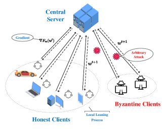
Figure 1: Illustration of the learning process of Fed-NGA on iteration number $t$.

2.2 Algorithm Description

To achieve our design goal, we develop Fed-NGA. In each iteration of Fed-NGA, the honest clients upload their own trained local gradient vector to the central server, while there are $B$ Byzantine clients that can send arbitrary vectors to bias the FL learning process. After receiving all uploaded vectors from all $M$ clients, the central server normalizes these uploaded vectors one-by-one and leverages the normalized vectors to update the global model parameter. With the global model parameter updated, the central server broadcasts it to all the $M$ clients in preparation for next iteration of training. Below, we give a full description of Fed-NGA (see Algorithm 1 and Figure 1). Its crucial steps are explained in detail as follows.

Local Updating: In the $t$th round of iteration, after receiving the global model parameter $w^{t}$ which is broadcasted from the central server, all honest clients $m,m\in\mathcal{M}\setminus\mathcal{B}$ select dataset $\mathcal{S}_{m},m\in\mathcal{M}\setminus\mathcal{B}$ to calculate their own local training gradient $\nabla F_{m}(w^{t})$. Meanwhile, all Byzantine clients $m,m\in\mathcal{B}$ can send an arbitrary vector or other malicious messages according to their own dataset and the global model parameter $w^{t}$. Let $g_{m}^{t}$ represent the vector (the local training gradient or malicious message) uploaded to the central server by client $m$, and we have

$$g_{m}^{t}=\left\{\begin{aligned} &{\nabla F_{m}(w^{t}),}&&{m\in\mathcal{M}\setminus\mathcal{B}}\\ &{\star,}&&{m\in\mathcal{B}}\end{aligned}\right.$$ (8)

Aggregation and Broadcasting: In the $t$th round of iteration, after receiving the vectors $g_{m}^{t},m\in\mathcal{M}$ from all the clients, the central server normalizes these vectors and updates the global model parameter $w^{t+1}$ with learning rate $\eta^{t}$, which is given as

$$w^{t+1}=w^{t}-\eta^{t}\sum_{m\in\mathcal{M}}\alpha_{m}\cdot\frac{g_{m}^{t}}{\left\lVert g_{m}^{t}\right\rVert}.$$ (9)

Then the central server broadcasts the global model parameter $w^{t+1}$ to all the clients for preparing the calculation in the $t+1$th round of iteration.

Based on the above description, Fed-NGA can achieve the design goal and output the global model parameter to approach the optimal solution of the problem in (1).

1:  Input: Initial global model parameter $w^{0}$, clients set $\mathcal{M}$, and the number of iteration number $T$.

2:  Output: Updated global model parameter $w^{T}$.

3:  % % Initialization

4:  Every client $m$ establishes its own set $\mathcal{S}_{m}$ for $m\in\mathcal{M}\setminus\mathcal{B}$.

5:  for $t=0,1,2,\cdots,T-1$ do

6:     for every client $m\in\mathcal{M}\setminus\mathcal{B}$ in parallel do

7:        Receive the global model $w^{t}$. Select dataset $\mathcal{S}_{m}$ to train local model and evaluate the local training gradient $\nabla F_{m}(w^{t})$. Set $g_{m}^{t}=\nabla F_{m}(w^{t})$ and upload $g_{m}^{t}$ to the central server.

8:     end for

9:     for every client $m\in\mathcal{B}$ in parallel do

10:        Receive the global model $w^{t}$. Generate an arbitrary vector or a malicious vector $g_{m}^{t}$ based on $w^{t}$ and dataset $\mathcal{S}_{m}$. Upload this vector $g_{m}^{t}$ to the central server.

11:     end for

12:     Receive all uploaded vectors $g_{m}^{t},m\in\mathcal{M}$. Normalize all uploaded vectors $g_{m}^{t}$. Update the global model parameter $w^{t+1}$ by

$$w^{t+1}=w^{t}-\eta^{t}\sum_{m\in\mathcal{M}}\alpha_{m}\cdot\frac{g_{m}^{t}}{\left\lVert g_{m}^{t}\right\rVert}.$$ (10)

13:     Broadcast the model parameter $w^{t+1}$ to all clients.

14:  end for

15:  Output the model parameter $w^{T}$.

Algorithm 1 Fed-NGA Algorithm

3 Theoretical Results

In this section, we theoretically analyze the robustness and convergence performance of Fed-NGA over the non-IID datasets. Below, we first present the necessary assumptions.

3.1 Assumption

First, we state some general assumptions in the work, which are also assumed in (Huang et al.,, 2023; Wu et al.,, 2023; Xiao and Ji,, 2023).

Assumption 3.1.

(Lipschitz Continuity). The loss function $f(w,s_{m,i})$ has $L$-Lipschitz continuity, i.e., for $\forall w_{1},w_{2}\in\mathbb{R}^{p}$, it follows that

$$f(w_{1},s_{m,i})-f(w_{2},s_{m,i})\leqslant\left\langle\nabla f(w_{2},s_{m,i}),w_{1}-w_{2}\right\rangle+\frac{L}{2}\left\lVert w_{1}-w_{2}\right\rVert^{2}.$$ (11)

which is equivalent to the following inequality,

$$\left\lVert\nabla f(w_{1},s_{m,i})-\nabla f(w_{2},s_{m,i})\right\rVert\leqslant L\left\lVert w_{1}-w_{2}\right\rVert.$$ (12)

With Assumption 3.1, it can be derived that all the local loss function $F_{m}(w)$ meets the Lipschitz continuity as they are linear combinations of the loss function $f(w,s_{m,i})$ (Huang et al.,, 2023). Similarly, the global loss function also has Lipschitz continuity. The Lipschitz continuity of a function permits it to be non-convex.

Assumption 3.2.

(Strongly Convex). The loss function $f(w,s_{m,i})$ is $\mu$-strongly convex, i.e., for $\forall w_{1},w_{2}\in\mathbb{R}^{p}$, it follows that

$$\left\lVert\nabla f(w_{1},s_{m,i})-\nabla f(w_{2},s_{m,i})\right\rVert\geqslant\mu\left\lVert w_{1}-w_{2}\right\rVert.$$ (13)

which is equivalent to the following inequality,

$$\left\langle\nabla f(w_{1},s_{m,i})-\nabla f(w_{2},s_{m,i}),w_{1}-w_{2}\right\rangle\geqslant\mu\left\lVert w_{1}-w_{2}\right\rVert^{2}.$$ (14)

Similarly, with Assumption 3.2, the local loss function $F_{m}(w)$ and the global loss function $F(w)$ are both strongly convex as they are linear combinations of $f(w,s_{m,i})$ for $m\in\mathcal{M}$ and $s_{m,i}\in\mathcal{S}_{m}$.

Assumption 3.3.

(Bounded Gradient). For $m\in\mathcal{M}$ and $\forall w\in\mathbb{R}^{p}$, the norm of gradients is uniformly bounded, i.e.,

$$\left\lVert\nabla F_{m}(w)\right\rVert\leqslant G.$$ (15)

With Assumption 3.3, it can be derived from the Jensen inequality that $\left\lVert\nabla F(w)\right\rVert$ is also upper bounded by $G$.

Assumption 3.4.

(Bounded Data Heterogeneity). For $m\in\mathcal{M}$, we define a representation of data heterogeneity by utilizing gradient direction, i.e.,

$$\theta_{m}=\left\lVert\frac{\nabla F_{m}(w)}{\left\lVert\nabla F_{m}(w)\right\rVert}-\frac{\nabla F(w)}{\left\lVert\nabla F(w)\right\rVert}\right\rVert,m\in\mathcal{M}.$$ (16)

We also assume the data heterogeneity is bounded, which implies

$$\theta_{m}\leqslant\theta,m\in\mathcal{M},$$ (17)

where $\theta$ is the heterogeneity upper bound.

In many literature such as (Huang et al.,, 2023; Li and Li,, 2023), they use $\left\lVert\nabla F_{m}(w)-\nabla F(w)\right\rVert$ to represent the data heterogeneity of $m$th client, which includes both direction and module deviation. In this paper, we relax it to be only with directional deviation, which allows more dataset distributional heterogeneity among all the clients. On the other hand, it can be checked that if and only if our defined heterogeneity upper bound $\theta$ goes to zero, the assumed dataset heterogeneity among all the clients will disappear.

3.2 Convergence Analysis

In this subsection, we present the analytical results of convergence on our proposed Fed-NGA. All the proofs are deferred to Appendix E and Appendix F.

3.2.1 With Lipschitz continuity only for loss function

Theorem 3.5.

With Assumption 3.1 and Assumption 3.4, with $\displaystyle\left(2-{(\theta)^{2}}/{2}\right)C_{\alpha}-1>0$, we have

$$\small\frac{1}{\sum_{t=0}^{T-1}\eta^{t}}\sum_{t=0}^{T-1}\eta^{t}\left\lVert\nabla F(w^{t})\right\rVert\leqslant\frac{F(w^{0})-F(w^{T})}{\left((2-\frac{(\theta)^{2}}{2})C_{\alpha}-1\right)\sum_{t=0}^{T-1}\eta^{t}}+\frac{L\sum_{t=0}^{T-1}(\eta^{t})^{2}}{2\left((2-\frac{(\theta)^{2}}{2})C_{\alpha}-1\right)\sum_{t=0}^{T-1}\eta^{t}}.$$ (18)

Proof.

Please refer to Appendix E. ∎

Remark 3.6.

For the case that the loss function exhibits Lipschitz continuity only, the bound of optimality gap and convergence rate in Theorem 3.5 reveal the impact of learning rate $\eta^{t}$, data heterogeneity upper bound $\theta$, and the intensity of Byzantine attack $\bar{C}_{\alpha}$ (i.e., $1-C_{\alpha}$) on the convergence performance for our proposed Fed-NGA. With the above results, to reduce the optimality gap and speed up the convergence rate, we need to first select an appropriate learning rate $\eta^{t}$. Then we analyze the robustness of Fed-NGA to Byzantine attacks on non-IID datasets under our selected learning rate. All the discussions are given as follows.

• With regard to the optimality gap, when $\displaystyle\lim_{T\rightarrow\infty}\sum_{t=1}^{T-1}\eta^{t}\rightarrow\infty$ and $\displaystyle\lim_{T\rightarrow\infty}\sum_{t=1}^{T-1}(\eta^{t})^{2}<\infty$, together with the prerequisite condition of Theorem 3.5, it can be derived that the average iteration error $\left({1}/{\sum_{t=0}^{T-1}\eta^{t}}\right)\cdot\sum_{t=0}^{T-1}\eta^{t}\left\lVert\nabla F(w^{t})\right\rVert$ converges to $0$. Therefore, $\displaystyle\min_{t}\left\lVert\nabla F(w^{t})-\nabla F(w^{*})\right\rVert$ will converge to zero.

• To further concrete convergence rate, we set $\displaystyle\eta^{t}={\eta}/{(t+1)^{1/2+\delta}}$, where $\delta$ is an arbitrary value lying between $(0,1/2)$, then the right-hand side of (18) is upper bounded by

  $$\mathcal{O}\left(\frac{F(w^{0})-F(w^{T})}{\left((2-\frac{(\theta)^{2}}{2})C_{\alpha}-1\right)\eta T^{\frac{1}{2}-\delta}}\right)+\mathcal{O}\left(\frac{L\eta(1+2\delta-2\delta T^{-2\delta})}{2\left((2-\frac{(\theta)^{2}}{2})C_{\alpha}-1\right)T^{\frac{1}{2}-\delta}}\right),$$ (19)

  which still converge to $0$ as $T\rightarrow\infty$, at a rate of $\mathcal{O}\left({1}/{T^{\frac{1}{2}-\delta}}\right)$.

• The required constraint $\displaystyle\left(2-{(\theta)^{2}}/{2}\right)C_{\alpha}-1>0$ discloses a trade-off between tolerable data heterogeneity and tolerable Byzantine attack intensity by our proposed Fed-NGA. In one extreme case, i.e., there is no data heterogeneity, which implies $\theta=0$. Then the upper limit of Fed-NGA’s ability to accommodate Byzantine attacks is $0.5$, i.e., our proposed Fed-NGA could converge as long as the dataset portion from Byzantine clients is less than 0.5. In another extreme case, there is no Byzantine clients, which means $C_{\alpha}=1$ and $\theta$ can be $\sqrt{2}$ at most. I.e, the diverse between ${\nabla F_{m}(w)}/{\left\lVert\nabla F_{m}(w)\right\rVert}$ and ${\nabla F(w)}/{\left\lVert\nabla F(w)\right\rVert}$ in this case could be $\pi/2$ at most. In the rest cases, the robustness to Byzantine attack can be traded with the tolerance to data heterogeneity by adjusting $\theta$ and $C_{\alpha}$.

3.2.2 With Lipschitz continuity and strongly convex for loss function

Theorem 3.7.

With Assumption 3.1, Assumption 3.2, Assumption 3.3, and Assumption 3.4, with $\gamma=2((\mu+L-L\cdot\theta)C_{\alpha}-L)/G>0$ and $w^{*}$ being the optimal solution of the problem in (1), there are two convergence results established as follows,

• With $\displaystyle\eta^{t}<{1}/{\gamma},t=0,1,\cdots,T-1$, the optimality gap $\left\lVert w^{T}-w^{*}\right\rVert^{2}$ is bounded as,

  $$\left\lVert w^{T}-w^{*}\right\rVert^{2}\leqslant\prod_{t=0}^{T-1}(1-\gamma\cdot\eta^{t})\left\lVert w^{0}-w^{*}\right\rVert^{2}+\sum_{t=0}^{T-2}(\eta^{t})^{2}\prod_{i=t+1}^{T-1}(1-\gamma\cdot\eta^{i})+(\eta^{T-1})^{2}.$$ (20)

• With $\eta^{T}\!<\!1/\gamma$, the iteration average error $\left(\!{1}/{\sum_{t=0}^{T}\eta^{t}}\!\right)\sum_{t=0}^{T}\eta^{t}\left\lVert w^{t}\!-\!w^{*}\right\rVert^{2}$ is bounded as

  $$\frac{1}{\sum_{t=0}^{T}\eta^{t}}\sum_{t=0}^{T}\eta^{t}\left\lVert w^{t}-w^{*}\right\rVert^{2}\leqslant\frac{\left\lVert w^{0}-w^{*}\right\rVert^{2}}{\gamma\sum_{t=0}^{T}\eta^{t}}+\frac{\sum_{t=0}^{T-1}(\eta^{t})^{2}}{\gamma\sum_{t=0}^{T}\eta^{t}}.$$ (21)

Proof.

Please refer to Appendix F for the proofs of the inequalities in (20) and (21). ∎

Remark 3.8.

For the case that the loss function exhibits both Lipschitz continuity and strong convexity, we state two convergence results in (20) and (21) to show the convergence. These two convergence results reflect the optimality gap and convergence rate of Fed-NGA under different learning rate setups, respectively. The trade-off between the robustness to Byzantine attacks intensity $\bar{C}_{\alpha}$ (also $1-C_{\alpha}$) and data heterogeneity indicator $\theta$ is also disclosed. Detailed discussions include:

• For the convergence result in (20), we set $\displaystyle\eta^{t}=\eta<{1}/{\gamma}$, and accordingly the optimality gap $\left\lVert w^{T}-w^{*}\right\rVert^{2}$ will converge to

  $$\mathcal{O}\left((1-\gamma\cdot\eta)^{T-1}\left\lVert w^{0}-w^{*}\right\rVert^{2}\right)+\mathcal{O}\left(\eta\frac{1-(1-\gamma\cdot\eta)^{T}}{\gamma}\right),$$ (22)

  which implies that the optimality gap will converge to $\displaystyle\mathcal{O}\left({\eta}/{\gamma}\right)$ as $T\rightarrow\infty$ at linear rate $\mathcal{O}\left((1-\gamma\cdot\eta)^{T-1}\right)$.

• For the convergence result in (21), similar to Remark 3.6, we set $\eta^{t}={\eta}/{(t+1)^{1/2+\delta}},\eta<{1}/{\gamma}$, then the right-hand side in (21) is upper bounded by

  $$\mathcal{O}\left(\frac{\left\lVert w^{0}-w^{*}\right\rVert^{2}}{\gamma\cdot\eta T^{1/2-\delta}}\right)+\mathcal{O}\left(\frac{\eta(1+2\delta-2\delta T^{-2\delta})}{\gamma\cdot T^{1/2-\delta}}\right),$$ (23)

  which will converge to $0$ as $T\rightarrow\infty$ at rate $\displaystyle\mathcal{O}\left({1}/{T^{1/2-\delta}}\right)$.

• Combining the above two discussions, if we set $\eta^{t}={\eta}/{(t+1)^{1/2+\delta}},\eta<{1}/{\gamma}$, then the optimality gap $\left\lVert w^{T}-w^{*}\right\rVert^{2}$ will converge to $0$ at rate $\displaystyle\mathcal{O}\left(\prod_{t=0}^{T-1}\left(1-{(\gamma\eta)}/{(t+1)^{1/2+\delta}}\right)\right)$, which shows that the optimality gap can approach to $0$ as $T\rightarrow\infty$ and is faster than $\displaystyle\mathcal{O}\left({1}/{T^{1/2-\delta}}\right)$.

• Similar with the discussion in Remark 3.6, the maximal tolerable intensity of Byzantine attacks is ${L}/{(L+\mu)}$ for IID datasets, and the maximal tolerable data heterogeneity $\theta<{(L+\mu)}/{L}$ when there is no Byzantine attack.

• Compared to Remark 3.6 after Theorem 3.5, the derived optimality gap after Theorem 3.7 can also converge to $0$ as $T\rightarrow\infty$ but at a faster rate $\displaystyle\mathcal{O}\left(\prod_{t=0}^{T-1}\left(1-{(\gamma\eta)}/{(t+1)^{1/2+\delta}}\right)\right)$, whereas the convergence rate in Remark 3.6 is $\mathcal{O}\left({1}/{T^{1/2-\delta}}\right)$. This advantage stems from the combination of Lipschitz continuity and strong convexity of the loss function.

4 Experiments

4.1 Setup

Dataset and Models: We experiment with MNIST dataset using LeNet (LeCun et al.,, 1998) and Multilayer Perceptron (MLP) (Yue et al.,, 2022) models. We split this dataset into $M$ non-IID training sets, which is relized by letting the label of data samples to conform to Dirichlet distribution with a concentration parameter $\beta$. A lager value of $\beta$ implies a more homogeneous distribution across each dataset. The loss function in LeNet and MLP can be regarded as non-convex and strongly convex, respectively. More details can be found in Appendix B.

Byzantine Attacks: The intensity level of Byzantine attack $\bar{C}_{\alpha}$ is set to 0, 0.1, 0.2, 0.3, 0.4 and we select three type of Byzantine attack, which are introduced as follow,

• Sign-flip attack: All Byzantine clients upload $-3*\sum_{m\in\mathcal{M}\setminus\mathcal{B}}g_{m}^{t}$ to the central server on iteration number $t$.

• Gaussian attack: All Byzantine attacks are selected as the Gaussian attack, which obeys $\mathcal{N}(0,90)$.

• Same-value attack: Each dimension of the Byzantine clients’ uploaded vector is set to 1.

Baselines: The convergence performance of five algorithms: Fed-NGA, FedAvg, Median, Krum and Geometric Median (GM) are compared. For the latter four algorithms, FedAvg is renowned in traditional FL and can be taken as a performance metric with no Byzantine attacks. Median, Krum, and GM utilizes coordinate-wise median, Krum, and geometric median to update the global model parameters over uploaded messages, respectively.

Performance Metrics: To assess the convergence performance, we measure the test accuracy, robustness, and running time. An algorithm would be better if it has higher test accuracy, is more tolerable to Byzantine attack, or has less running time.

4.2 Results for Training Performance

Table 2: The part results of max test accuracy on 10000 iterations for five algorithms with different types, levels of Byzantine attack, and concentration parameter on two learning models.

Attack type			Sign-flip attack					Gaussian attack					Same-value attack
Model	$\beta$	$\bar{C}_{\alpha}$	Ours	FedAvg	Median	Krum	GM	Ours	FedAvg	Median	Krum	GM	Ours	FedAvg	Median	Krum	GM
LeNet	0.6	0	98.38	98.77	98.32	98.05	97.62	98.38	98.82	97.95	98.04	97.62	98.38	98.79	98.14	98.23	97.63
		0.2	97.96	11.35	98.01	98.11	97.59	98.09	41.13	97.97	98.10	97.56	93.06	11.35	95.73	95.78	92.86
		0.4	97.64	9.80	97.84	98.15	97.52	97.67	36.36	98.14	98.22	97.53	83.44	10.28	81.84	78.55	80.99
	0.2	0	97.95	98.92	96.13	95.90	97.59	97.95	98.85	96.01	95.92	97.59	97.95	98.88	96.44	95.92	97.59
		0.2	97.33	9.82	95.79	95.93	97.60	97.45	39.71	95.83	95.74	97.56	89.59	11.35	93.35	92.96	88.68
		0.4	96.75	9.80	96.03	96.09	97.51	96.79	29.18	96.64	96.39	97.50	80.43	10.28	50.88	50.63	19.34
MLP	0.6	0	97.51	97.60	96.98	96.95	94.03	97.51	97.60	96.98	96.95	94.03	97.51	97.61	96.98	96.95	94.03
		0.2	97.03	11.35	96.80	96.78	94.00	97.10	85.79	96.77	96.66	94.01	92.17	11.35	94.18	94.01	92.11
		0.4	96.17	12.03	96.40	96.23	93.68	96.20	88.23	96.52	96.44	93.86	87.56	11.35	82.13	82.18	85.08
	0.2	0	97.05	97.59	95.25	95.40	94.00	97.05	97.59	95.25	95.40	94.00	97.05	97.59	95.25	95.40	94.00
		0.2	96.20	9.82	94.52	94.92	93.66	96.44	85.76	95.28	95.42	94.02	91.05	9.83	90.47	90.49	90.95
		0.4	95.37	10.32	95.65	95.16	93.63	95.08	86.50	94.85	95.42	93.57	85.25	10.12	61.29	61.26	81.09

We begin our analysis with Table 2, which presents the test accuracy of five algorithms under varying levels of Byzantine attack intensity, $\bar{C}_{\alpha}$, across different concentration parameters, $\beta$ , and for two learning models. Further details are available in Tab 3. The data indicates that Fed-NGA secures the second-highest accuracy in scenarios devoid of Byzantine attacks, with FedAvg leading the pack. Additionally, Fed-NGA consistently achieves the second-highest accuracy for both Sign-flip and Gaussian attacks, with a minimal performance gap of 0.3% to 0.7% compared to the top-performing algorithm. In the context of Same-value attacks, Fed-NGA excels under conditions of intense attacks and significant data heterogeneity, boasting an improvement of 25% to 30% over competing algorithms. Regarding data heterogeneity, Fed-NGA ranks as the second most stable algorithm for Sign-flip and Gaussian attacks (with GM being the most stable), and it stands out as the most stable one for Same-value attacks.

Additionally, the performance of Fed-NGA and other algorithms in different settings is ploted and analyzed in Appendix C.

Figure 2: Running time for five algorithms with iteration number $T=10000$.

4.3 Results for Running Time

To assess the running time, we conducted a comparative analysis of Fed-NGA against baseline algorithms by calculating the code execution time for the five aggregation algorithms over 10,000 iterations under a Gaussian attack with $\bar{C}_{\alpha}=0.2$. The results are depicted in Fig 2. As illustrated in Fig 2, FedAvg requires the least amount of time for its aggregation process, with Fed-NGA ranking as the second fastest. The time consumed by GM is 45-fold, and Median is 150-fold that of our proposed Fed-NGA. The duration taken by Krum is disproportionately high in comparison to the others. Among all five algorithms, Fed-NGA takes only 40% more time than FedAvg, yet it achieves robustness against Byzantine attacks while maintaining commendable test accuracy.

5 Conclusion

In this paper, we propose a new FL framework Fed-NGA, which normalizes the uploaded local gradients to be a norm-one vector before aggregation, and only has a time complexity of $\mathcal{O}(pM)$ that outperforms all the existing Byzantine-robust methods and is comparable with FedAvg. Non-convex loss function and dataset heterogeneity are both considered, not like existing literature that can only deal with one at most. Zero optimality gap is reached at rate $\mathcal{O}(1/T^{\frac{1}{2}-\delta})$ in this case. A new trade-off between tolerable Byzantine intensity and data heterogeneity is also disclosed. In case with strongly convex loss function and heterogeneous dataset, the zero optimality gap achieving rate is improved to be linear. Extensive experiments are conducted to verify the advantages of Fed-NGA in terms of convergence performance and time complexity over existing methods.

Appendix A Notation

In this part, we introduce the notation in this paper. $\left\langle x,y\right\rangle$ denotes the inner product of the vectors $x$ and $y$. $\left\lVert x\right\rVert$ stands for the Euclidean norm $\left\lVert x\right\rVert_{2}$. For convenience, we also define

$$g^{t}=\sum_{m\in\mathcal{M}}\alpha_{m}\cdot\frac{g_{m}^{t}}{\left\lVert g_{m}^{t}\right\rVert},$$ (24)

which states the weighted sum of the normalized local gradients from all clients on the $t$th round of iteration.

Appendix B Implementation Details

To carry out our experiments, we set up a machine learning environments in PyTorch 2.2.2 on Ubuntu 20.04, powered by four RTX A6000 GPUs and one AMD 7702 CPU.

B.1 Dataset

We conduct experiments by leveraging MNIST dataset, which includes a training set and a test set. The training set contains 60000 samples and the test set contains 10000 samples, each sample of which is a 28 $\times$ 28 pixel grayscale image. We split this dataset into $M$ non-IID training sets, which is realized by letting the label of data samples to conform to Dirichlet distribution. The extent of non-IID can be adjusted by tuning the concentration parameter $\beta$ of Dirichlet distribution.

B.2 Model

For training problems with non-convex and strongly convex loss functions, we adopt LeNet and Multilayer Perceptron (MLP) model, respectively. The introduction of these two models are as follows:

• LeNet: The LeNet model is one of the earliest published convolutional neural networks. For the experiments, we are going to train a LeNet model with two convolutional layers (both kernel size are 5 and the out channel of first one is 6 and second one is 16), two pooling layers (both kernel size are 2 and stride are 2), and three fully connected layer (the first one is (16 * 4 * 4, 120), the second is (120, 60) and the last is (60, 10)) like in (LeCun et al.,, 1998). Cross-entropy function is taken as the training loss.

• MLP: The MLP model is a machine learning model based on Feedforward Neural Network that can achieve high-level feature extraction and classification. To promise strong convexity for the loss function, we configure the MLP model to be with three connected layers (the first one is (28 * 28, 200), the second is (200, 200) and the last is (200, 10)) like in (Yue et al.,, 2022) and take the cross-entropy function as the training loss.

B.3 Hyperparameters

We assume $M=100$ and the batchsize of all the experiments is 512. The concentration parameter $\beta$ is set to 0.6, 0.4 and 0.2. In default, the iteration number $T=10000$. In terms of learning rate, we adopt $\eta^{t}=0.02$ for all methods to be fair.

Appendix C Addition Results

Table 3: The max test accuracy of 10000 iteration number of five algorithm with different types, levels of Byzantine attack, and concentration parameter on two learning models.

Attack type			Sign-flip attack					Gaussian attack					Same-value attack
Model	$\beta$	$\bar{C}_{\alpha}$	Ours	FedAvg	Median	Krum	GM	Ours	FedAvg	Median	Krum	GM	Ours	FedAvg	Median	Krum	GM
LeNet	0.6	0	98.38	98.77	98.32	98.05	97.62	98.38	98.82	97.95	98.04	97.62	98.38	98.79	98.14	98.23	97.63
		0.1	98.19	49.90	98.19	98.12	97.56	98.18	57.91	98.02	98.13	97.60	96.84	10.09	97.54	97.43	96.69
		0.2	97.96	11.35	98.01	98.11	97.59	98.09	41.13	97.97	98.10	97.56	93.06	11.35	95.73	95.78	92.86
		0.3	97.78	10.28	98.20	98.19	97.64	97.92	31.09	98.03	98.03	97.55	87.33	11.35	91.78	91.06	85.43
		0.4	97.64	9.80	97.84	98.15	97.52	97.67	36.36	98.14	98.22	97.53	83.44	10.28	81.84	78.55	80.99
	0.4	0	98.30	98.83	97.50	97.62	97.72	98.30	98.88	97.40	97.40	97.73	98.30	98.85	97.60	97.48	97.72
		0.1	98.09	9.80	97.52	96.91	97.63	98.15	71.25	97.49	97.85	97.78	96.51	11.35	96.80	97.10	96.37
		0.2	98.00	10.10	97.48	97.61	97.75	97.97	38.85	97.45	97.33	97.72	92.37	11.35	95.17	95.31	92.10
		0.3	97.70	10.09	97.07	97.31	97.57	97.81	32.34	97.81	97.45	97.63	86.85	10.10	91.61	90.80	87.18
		0.4	97.44	9.80	97.59	97.53	97.62	97.33	25.21	97.49	97.34	97.55	84.05	10.28	66.72	66.68	76.91
	0.2	0	97.95	98.92	96.13	95.90	97.59	97.95	98.85	96.01	95.92	97.59	97.95	98.88	96.44	95.92	97.59
		0.1	97.75	26.37	96.62	96.15	97.58	97.74	63.98	96.25	96.19	97.60	95.68	11.35	94.35	94.61	95.80
		0.2	97.33	9.82	95.79	95.93	97.60	97.45	39.71	95.83	95.74	97.56	89.59	11.35	93.35	92.96	88.68
		0.3	97.11	9.82	95.88	95.55	97.51	97.24	40.80	95.48	95.64	97.73	82.59	11.35	74.82	70.15	81.02
		0.4	96.75	9.80	96.03	96.09	97.51	96.79	29.18	96.64	96.39	97.50	80.43	10.28	50.88	50.63	19.34
MLP	0.6	0	97.51	97.60	96.98	96.95	94.03	97.51	97.60	96.98	96.95	94.03	97.51	97.61	96.98	96.95	94.03
		0.1	97.25	50.63	96.78	96.94	93.91	97.25	88.31	96.86	96.95	94.00	94.83	11.35	95.53	95.48	93.52
		0.2	97.03	11.35	96.80	96.78	94.00	97.10	85.79	96.77	96.66	94.01	92.17	11.35	94.18	94.01	92.11
		0.3	96.72	10.10	96.61	96.69	93.79	96.77	85.87	96.82	96.78	93.94	90.26	10.15	90.14	90.08	89.81
		0.4	96.17	12.03	96.40	96.23	93.68	96.20	88.23	96.52	96.44	93.86	87.56	11.35	82.13	82.18	85.08
	0.4	0	97.42	97.58	96.46	96.38	94.01	97.42	97.58	96.46	96.38	94.01	97.42	97.58	96.46	96.38	94.01
		0.1	97.16	9.80	96.28	96.26	93.87	97.25	86.86	96.36	96.43	94.02	94.69	11.35	94.95	94.67	93.41
		0.2	96.86	11.35	96.43	96.40	93.94	96.93	87.23	96.38	96.27	93.90	91.83	11.35	93.02	92.94	91.73
		0.3	96.47	10.10	96.57	96.45	93.75	96.50	85.52	96.28	96.08	94.00	89.53	11.35	87.85	87.87	89.08
		0.4	96.05	9.82	96.11	95.97	93.72	95.98	85.49	96.40	96.19	93.92	87.11	11.35	72.78	72.69	84.02
	0.2	0	97.05	97.59	95.25	95.40	94.00	97.05	97.59	95.25	95.40	94.00	97.05	97.59	95.25	95.40	94.00
		0.1	96.68	18.08	95.09	95.74	93.85	96.83	87.11	95.44	95.80	93.89	93.71	11.35	92.87	92.75	93.18
		0.2	96.20	9.82	94.52	94.92	93.66	96.44	85.76	95.28	95.42	94.02	91.05	9.83	90.47	90.49	90.95
		0.3	96.09	10.10	95.25	95.38	94.00	95.97	86.74	95.25	95.44	93.97	88.73	10.32	84.34	84.14	88.14
		0.4	95.37	10.32	95.65	95.16	93.63	95.08	86.50	94.85	95.42	93.57	85.25	10.12	61.29	61.26	81.09

In this section, we examine the impact of different type of Byzantine attack, the intensity level of Byzantine attack, and degree of data heterogeneity for these five algorithms on two learning models. We first explore the impact of hyperparameters on five algorithms and then discuss the comparison on five algorithms for training performance by Tab 3 and Fig 3 - 20.

C.1 Results for Impact of Hyperparameters

Degree of data heterogeneity: In the context of Sign-flip attack and Gaussian attack, Tab 3 demonstrates Fed-NGA maintains stability across various settings of $\beta$. Specifically, the test accuracy discrepancy for Fed-NGA ranges merely from 0.03% $\sim$ 0.1% as $\beta$ decreases from 0.6 to 0.2. In contrast, the Median and Krum algorithms exhibit heightened sensitivity to data heterogeneity, with potential test accuracy disparities reaching up to 2%. Although GM remains stable in the face of data heterogeneity, its performance lags behind Fed-NGA when applied to the MLP model. During Same-value attacks, Fed-NGA surpasses other algorithms, particularly under conditions of significant data heterogeneity, as evidenced in Tab 3 and Fig 15, 17, 18, and 20. Fig 17 reveals that Median, Krum, and GM fail to converge on the LeNet model, and they only achieve low test accuracy on the MLP model as shown in Fig 20. Conversely, Fed-NGA consistently exhibits robust performance amidst high data heterogeneity and intense levels of Byzantine attacks. The test accuracy gap for Median, Krum, and GM spans a significant range of 20% $\sim$ 50%, whereas Fed-NGA maintains a maximum differential of merely 3%.

Intensity level of Byzantine attack: Regarding Sign-flip attack and Gaussian attack, all algorithms, with the exception of FedAvg, exhibit commendable performance across varying sets of $\bar{C}_{\alpha}$. In the case of Same-value attacks, Fig 15 - 20 illustrate that Fed-NGA consistently surpasses competing algorithms, especially under severe levels of Byzantine attacks. The disparity in test accuracy between Fed-NGA and the other algorithms can be as substantial as 3% $\sim$ 60% for the LeNet model, and 2.5% $\sim$ 20% for the MLP model. Across all three types of attacks, Fed-NGA emerges as the superior performer.

C.2 Comparison Results for Training Performance

Without Byzantine attack: For all varied hyperparameter configurations, FedAvg emerges as the top performer among the five algorithms in scenarios devoid of Byzantine attacks, with our proposed Fed-NGA closely trailing.

Sign-flip attack: Fed-NGA exhibits robust performance in scenarios characterized by low-intensity Byzantine attacks and high data heterogeneity. In other scenarios, while our proposed Fed-NGA may not claim the top spot, the performance gap from the leading algorithm does not exceed 0.5%.

Gaussian attack: The outcomes are largely analogous to those observed in the Sign-flip attack, with the exception that FedAvg’s test accuracy can occasionally soar to 85% under low-intensity Byzantine attacks.

Same-value attack: Fed-NGA outshines all five algorithms in situations of high data heterogeneity and intense Byzantine attacks. Despite occasional test accuracy discrepancies of approximately 2% between Fed-NGA and the Median (Krum), these two algorithms exhibit markedly inferior performance under severe Byzantine attack conditions, with test accuracy gaps ranging from 2.5% to 30% when compared to our proposed Fed-NGA. Overall, Fed-NGA demonstrates superior performance.

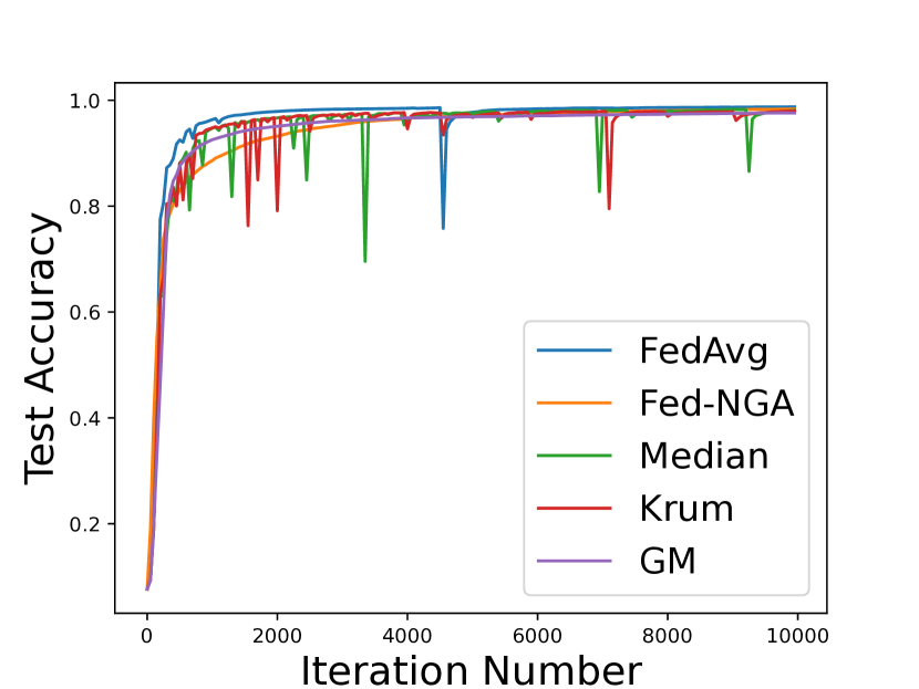
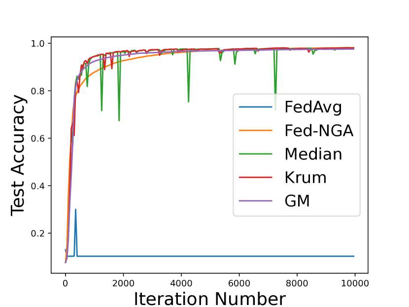
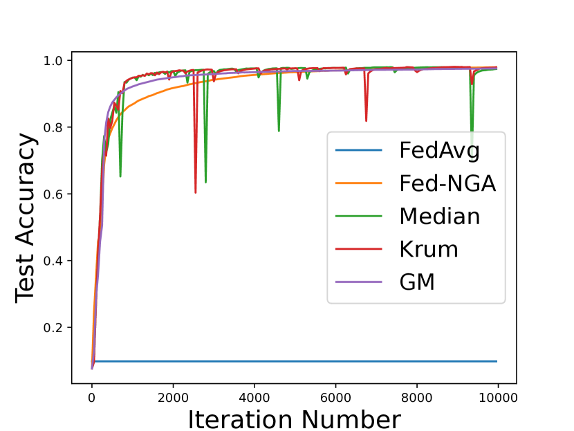
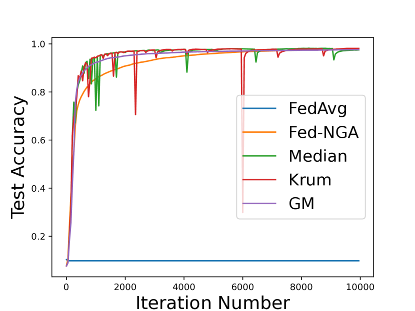
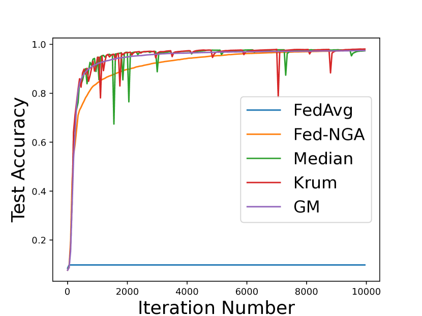
Figure 3: Test accuracy of LeNet with sign-flip attacks for $\beta=0.6$. The intensity levels of Byzantine attack $\bar{C}_{\alpha}$ are 0, 0.1, 0.2, 0.3, 0.4 in order.

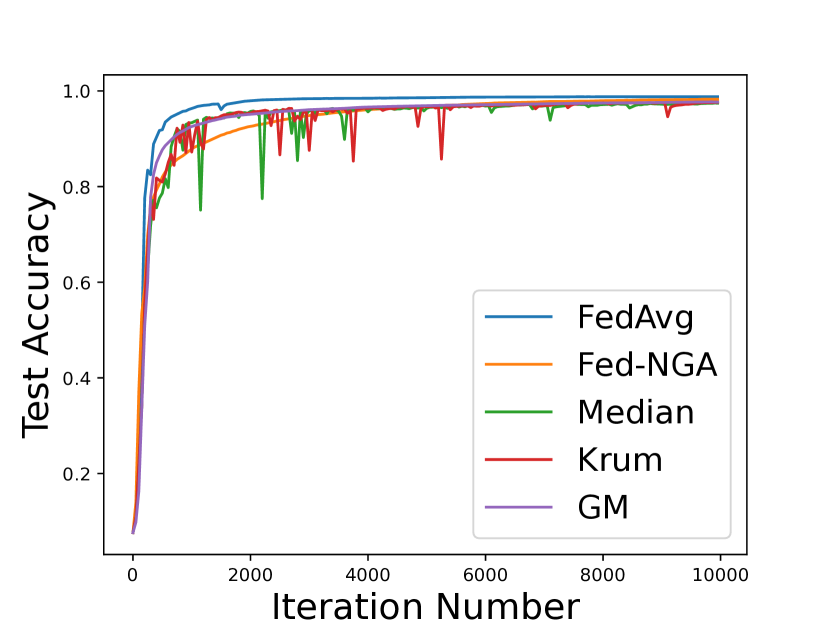
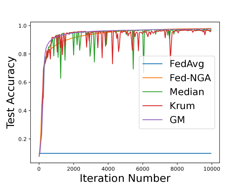
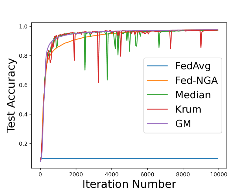
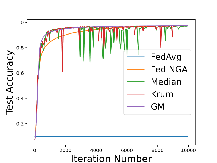
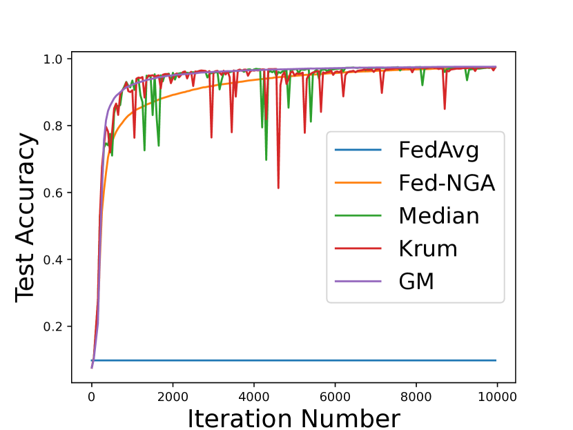
Figure 4: Test accuracy of LeNet with sign-flip attacks for $\beta=0.4$. The intensity levels of Byzantine attack $\bar{C}_{\alpha}$ are 0, 0.1, 0.2, 0.3, 0.4 in order.

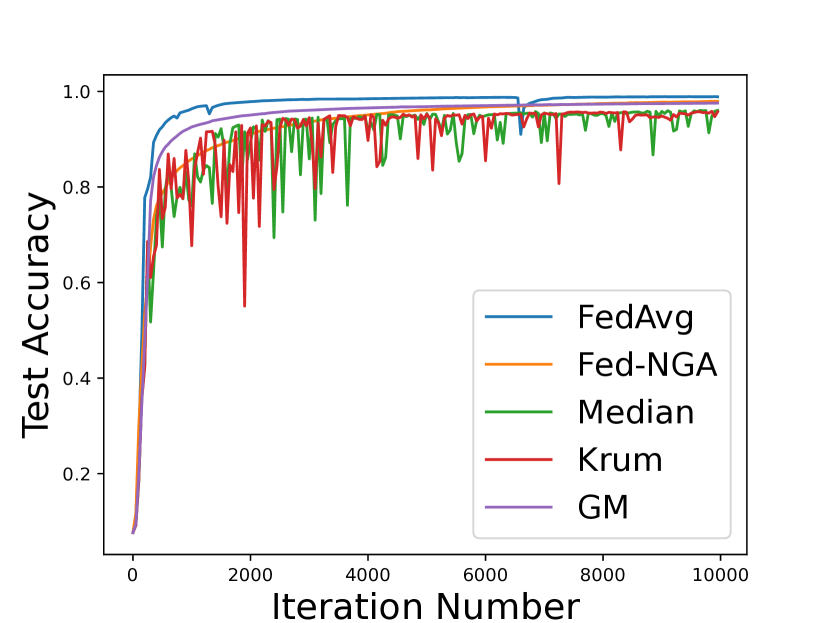
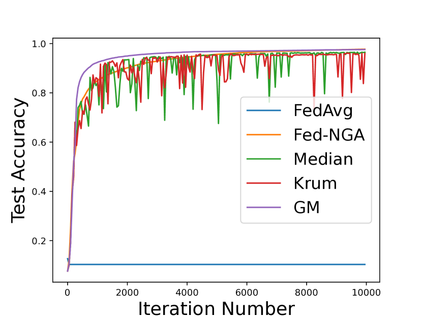
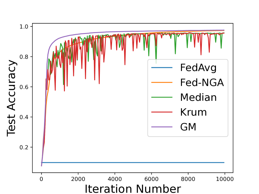
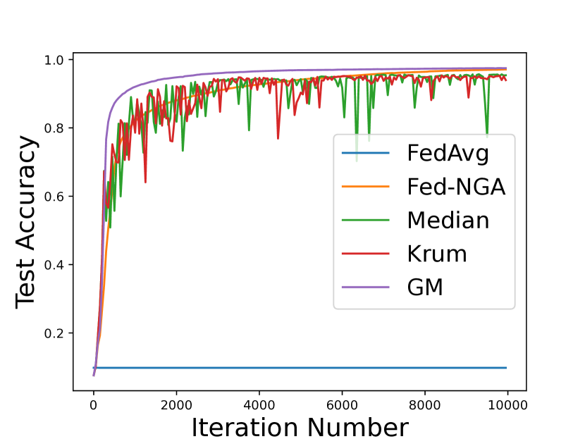
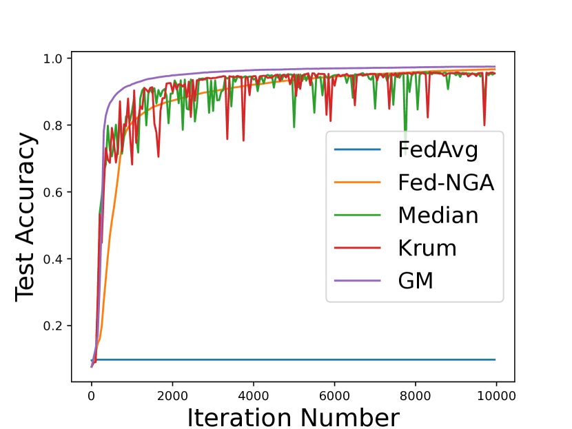
Figure 5: Test accuracy of LeNet with sign-flip attacks for $\beta=0.2$. The intensity levels of Byzantine attack $\bar{C}_{\alpha}$ are 0, 0.1, 0.2, 0.3, 0.4 in order.

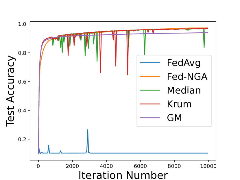
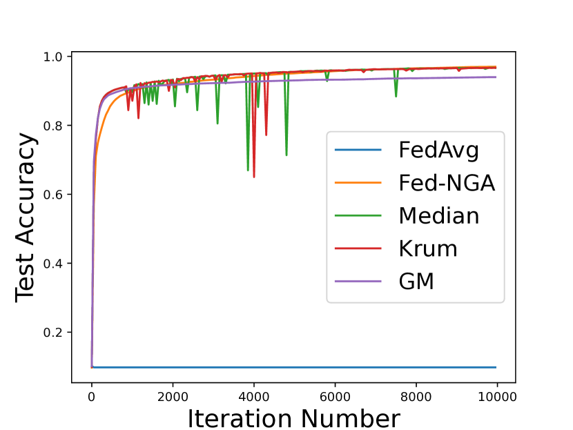
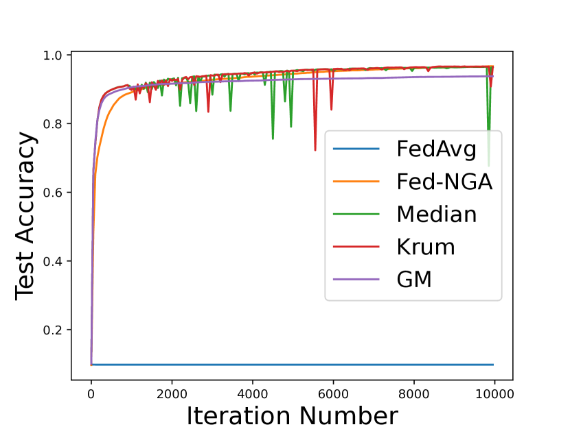
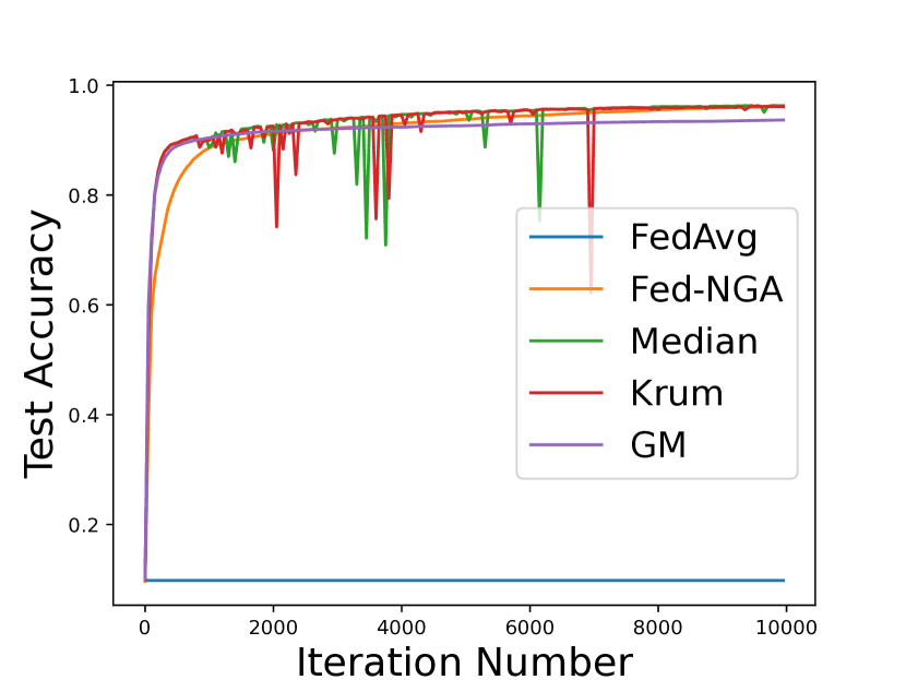
Figure 6: Test accuracy of MLP with sign-flip attacks for $\beta=0.6$. The intensity levels of Byzantine attack $\bar{C}_{\alpha}$ are 0, 0.1, 0.2, 0.3, 0.4 in order.

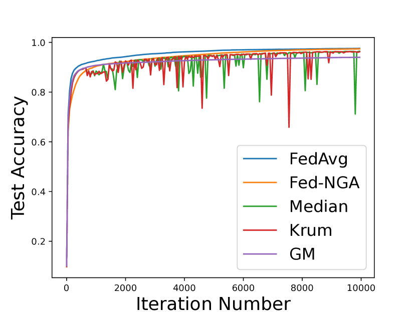
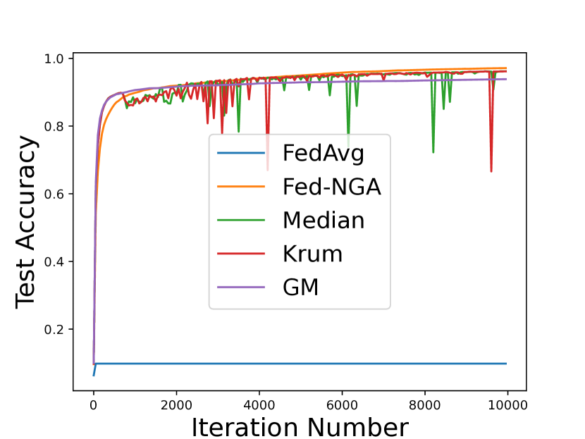
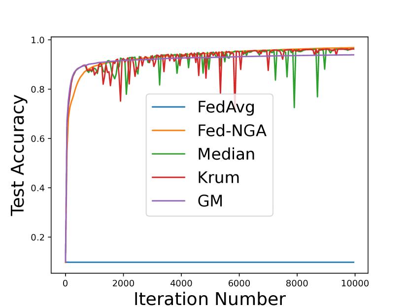
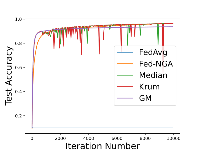
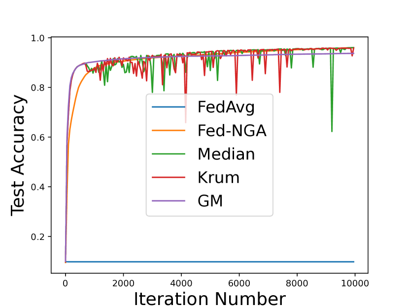
Figure 7: Test accuracy of MLP with sign-flip attacks for $\beta=0.4$. The intensity levels of Byzantine attack $\bar{C}_{\alpha}$ are 0, 0.1, 0.2, 0.3, 0.4 in order.

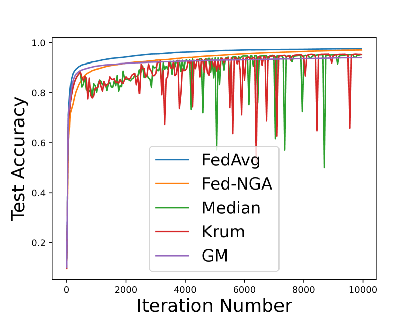
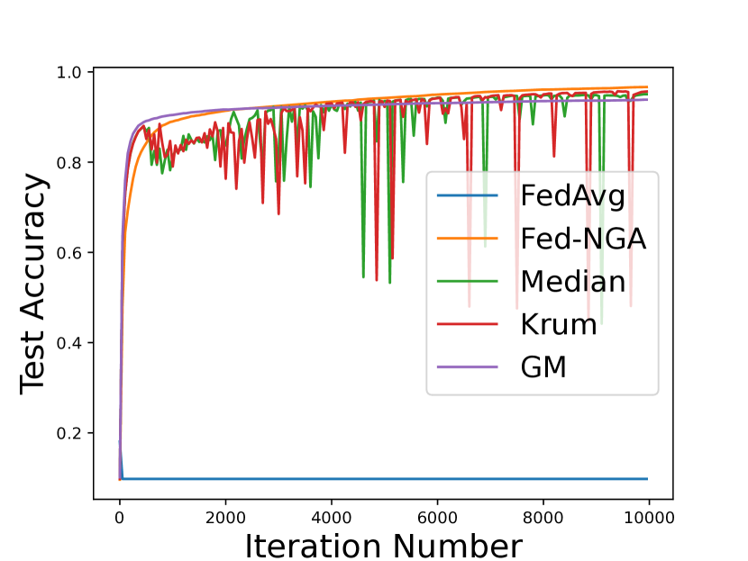
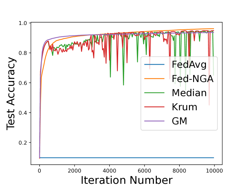
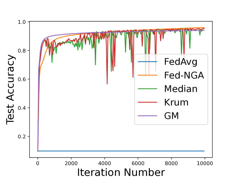
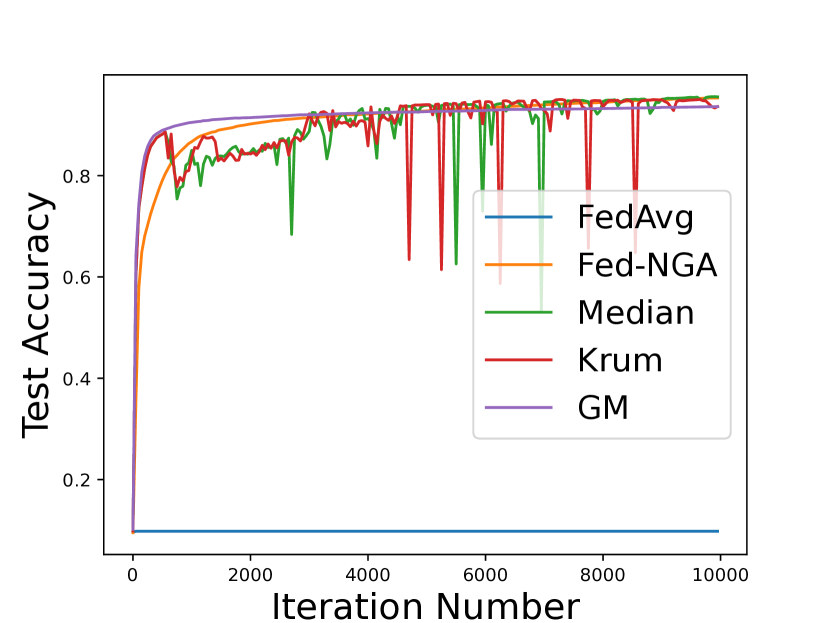
Figure 8: Test accuracy of MLP with sign-flip attacks for $\beta=0.2$. The intensity levels of Byzantine attack $\bar{C}_{\alpha}$ are 0, 0.1, 0.2, 0.3, 0.4 in order.

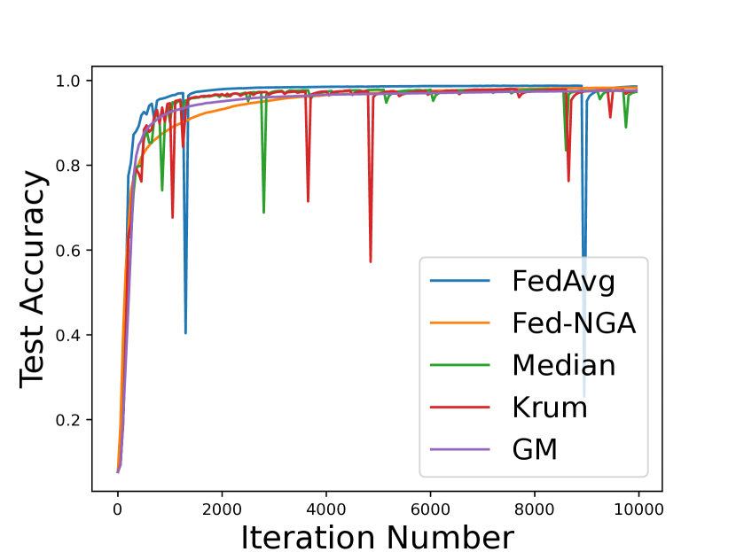
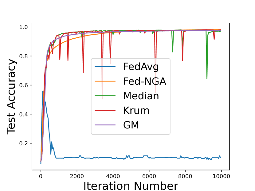
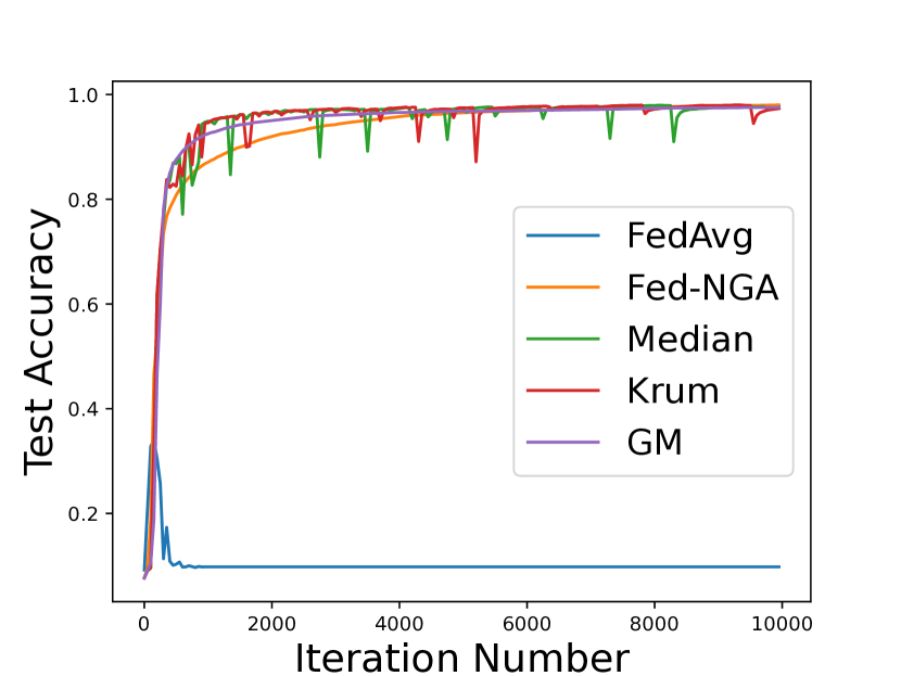
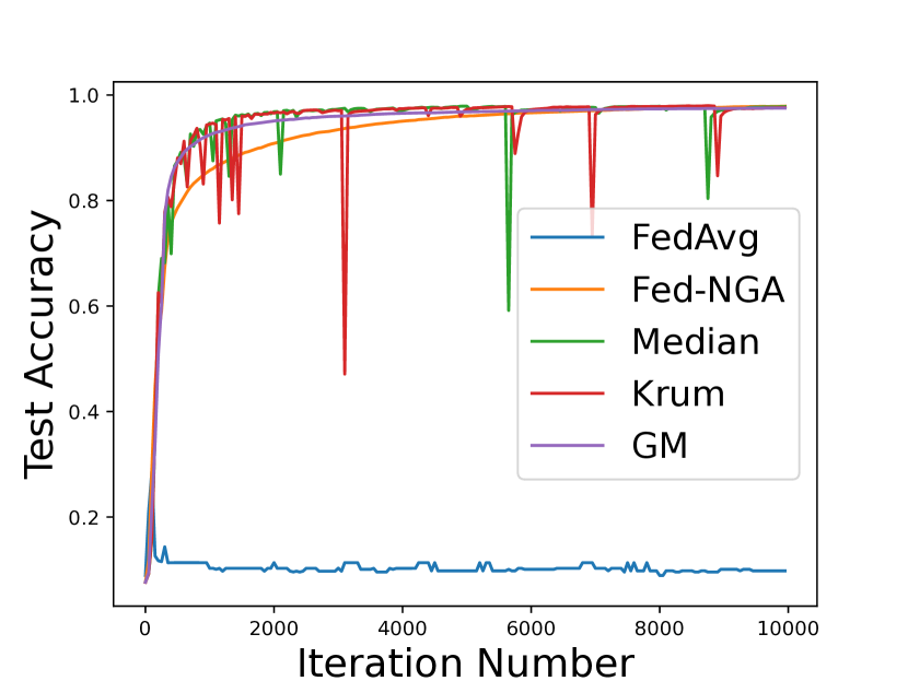
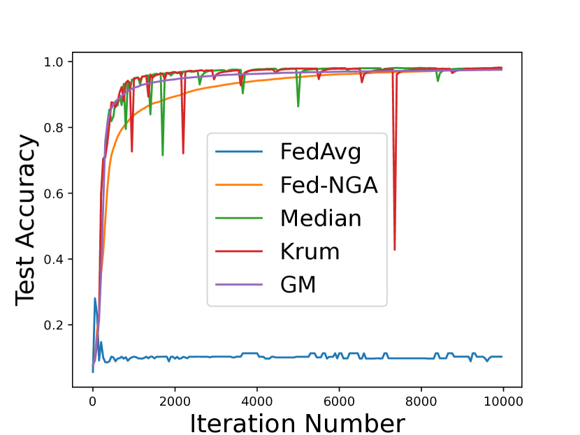
Figure 9: Test accuracy of LeNet with Gaussian attacks for $\beta=0.6$. The intensity levels of Byzantine attack $\bar{C}_{\alpha}$ are 0, 0.1, 0.2, 0.3, 0.4 in order.

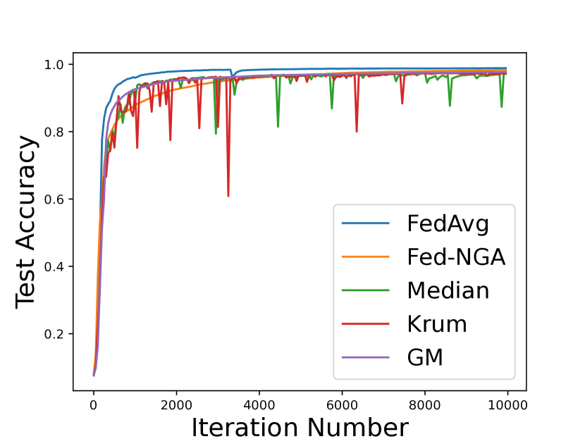
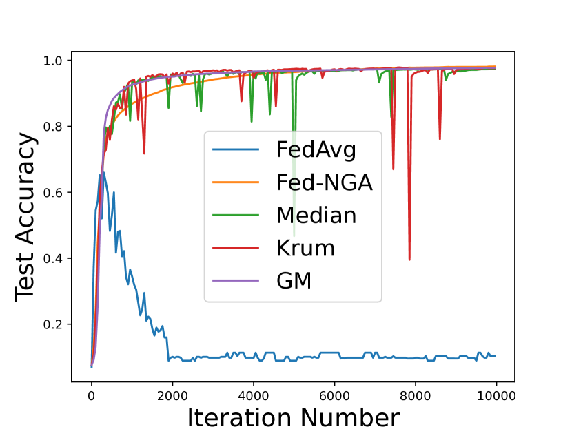
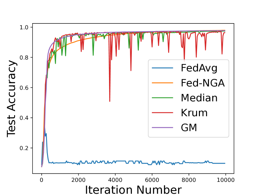
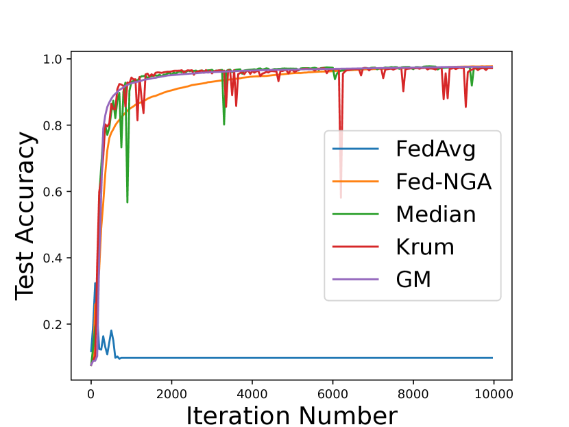
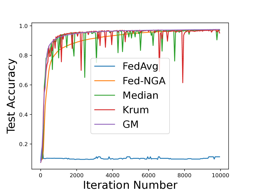
Figure 10: Test accuracy of LeNet with Gaussian attacks for $\beta=0.4$. The intensity levels of Byzantine attack $\bar{C}_{\alpha}$ are 0, 0.1, 0.2, 0.3, 0.4 in order.

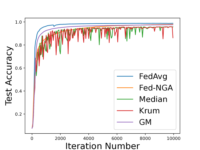
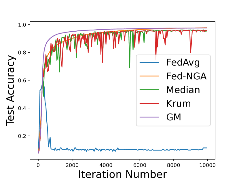
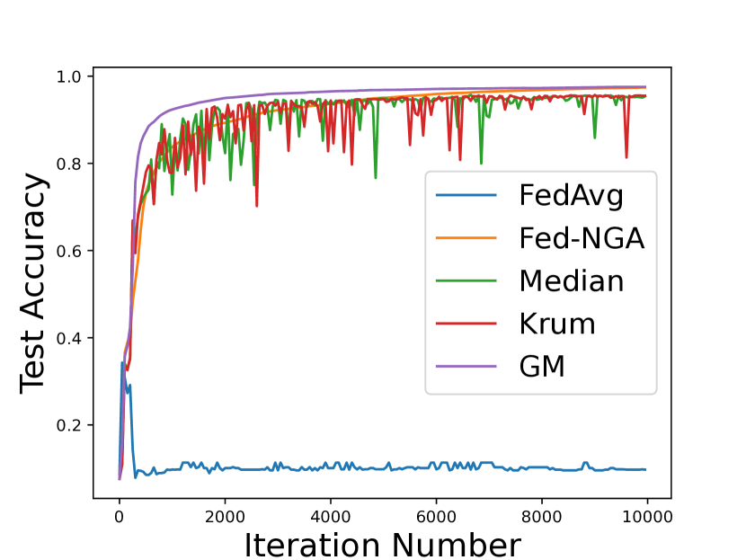
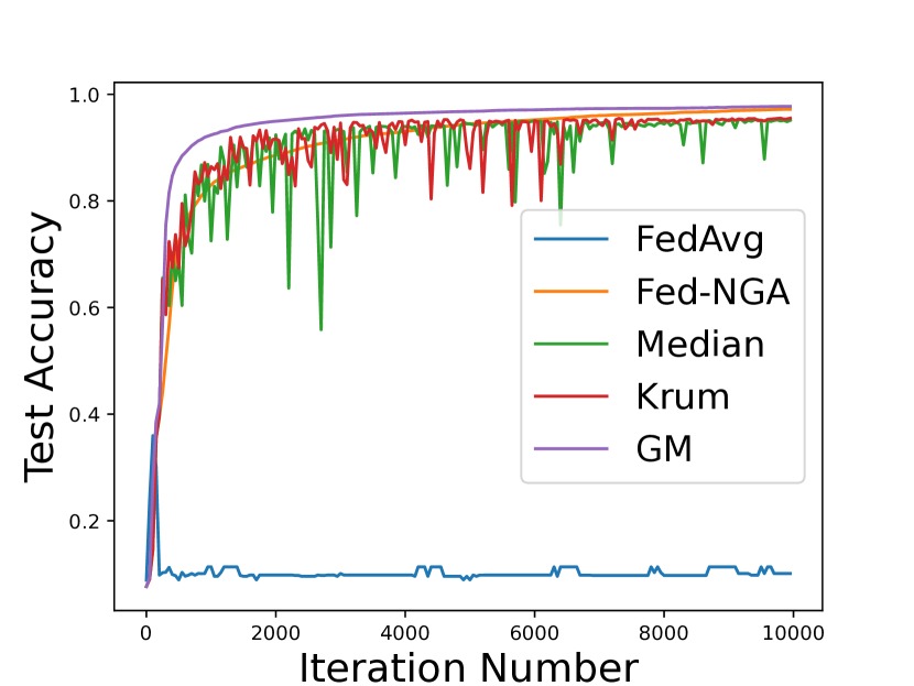
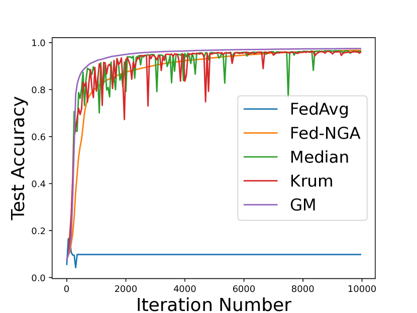
Figure 11: Test accuracy of LeNet with Gaussian attacks for $\beta=0.2$. The intensity levels of Byzantine attack $\bar{C}_{\alpha}$ are 0, 0.1, 0.2, 0.3, 0.4 in order.

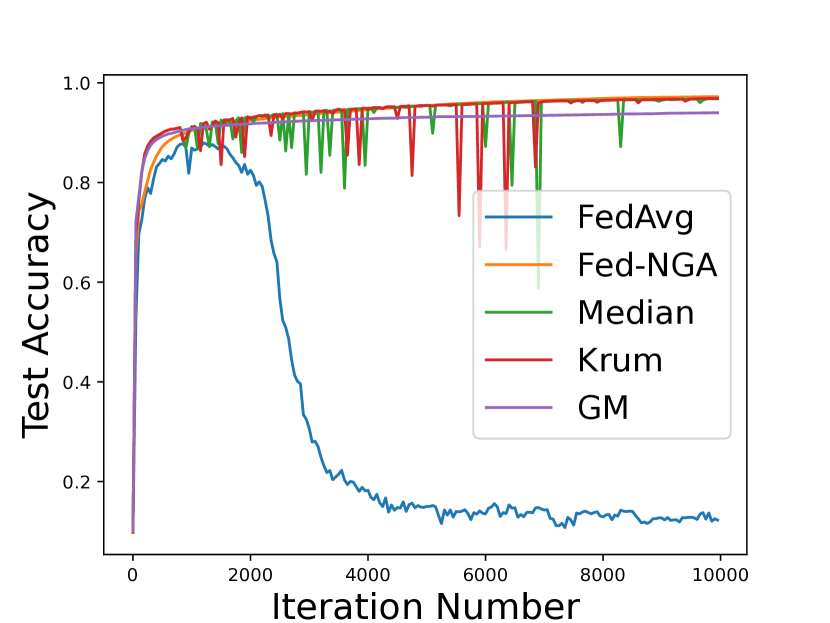
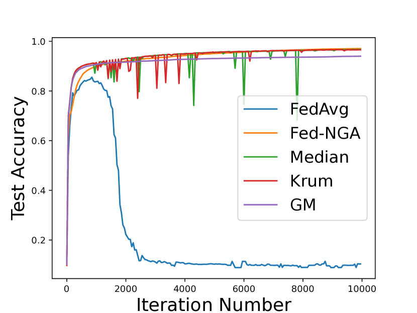
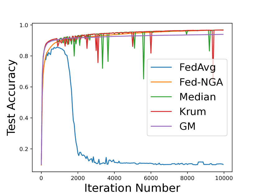
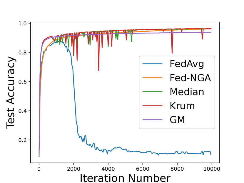
Figure 12: Test accuracy of MLP with Gaussian attacks for $\beta=0.6$. The intensity levels of Byzantine attack $\bar{C}_{\alpha}$ are 0, 0.1, 0.2, 0.3, 0.4 in order.

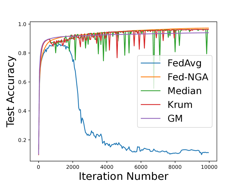
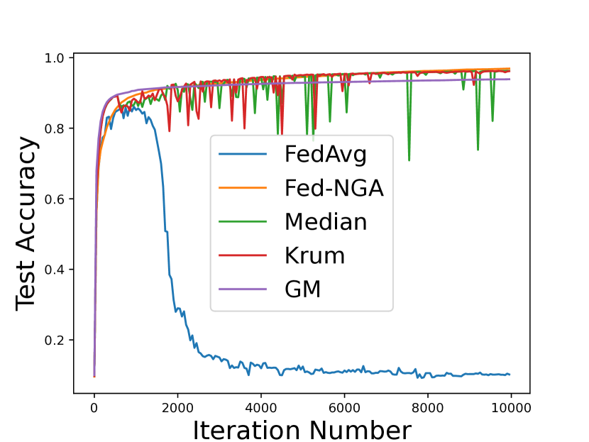
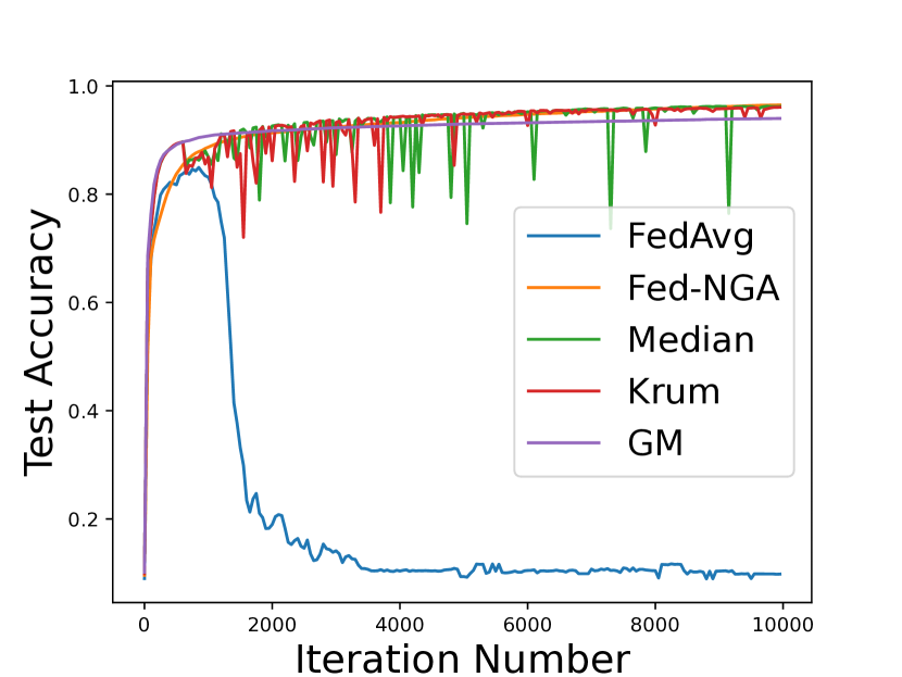
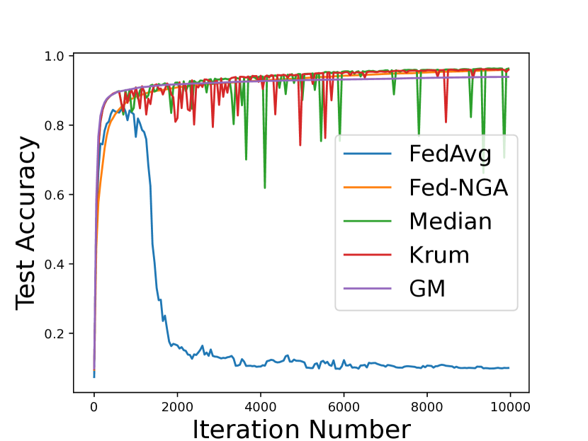
Figure 13: Test accuracy of MLP with Gaussian attacks for $\beta=0.4$. The intensity levels of Byzantine attack $\bar{C}_{\alpha}$ are 0, 0.1, 0.2, 0.3, 0.4 in order.

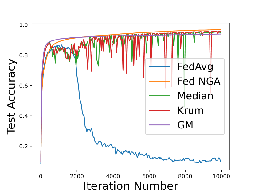
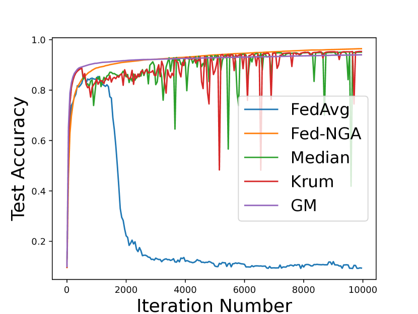
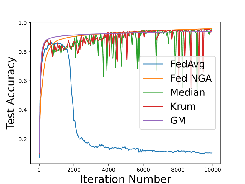
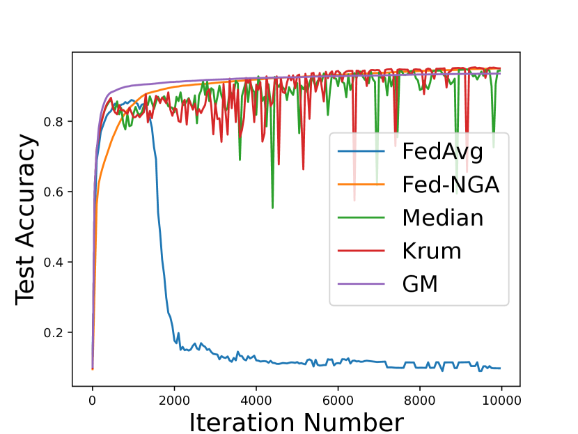
Figure 14: Test accuracy of MLP with Gaussian attacks for $\beta=0.2$. The intensity levels of Byzantine attack $\bar{C}_{\alpha}$ are 0, 0.1, 0.2, 0.3, 0.4 in order.

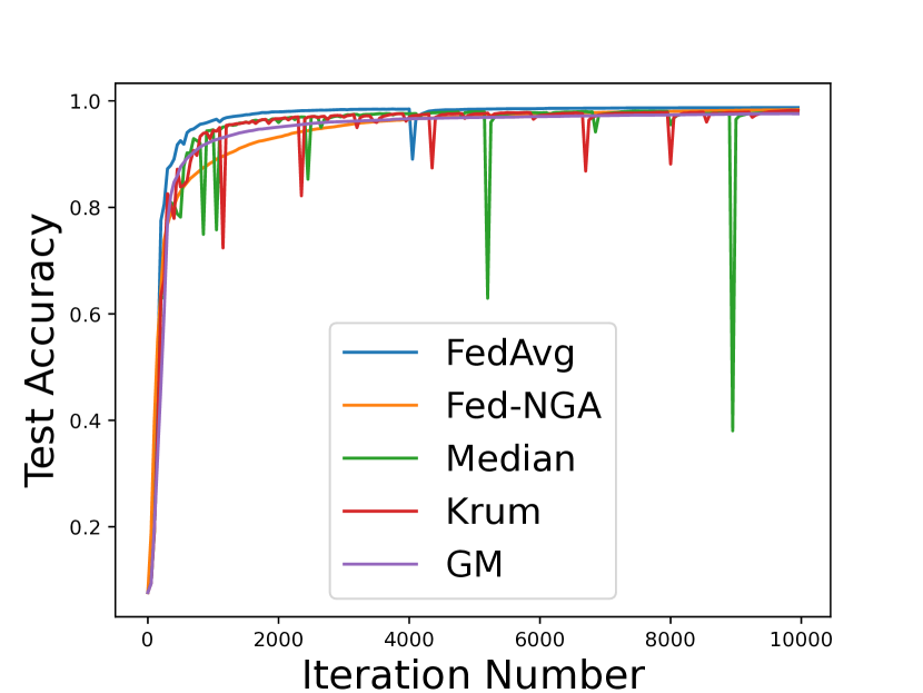
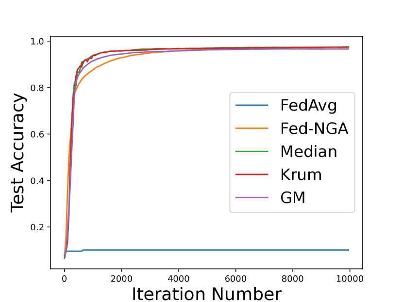
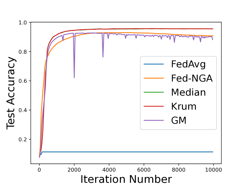
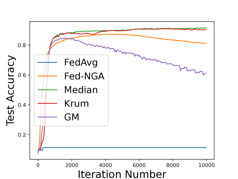
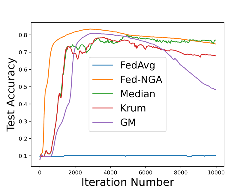
Figure 15: Test accuracy of LeNet with Same-value attacks for $\beta=0.6$. The intensity levels of Byzantine attack $\bar{C}_{\alpha}$ are 0, 0.1, 0.2, 0.3, 0.4 in order.

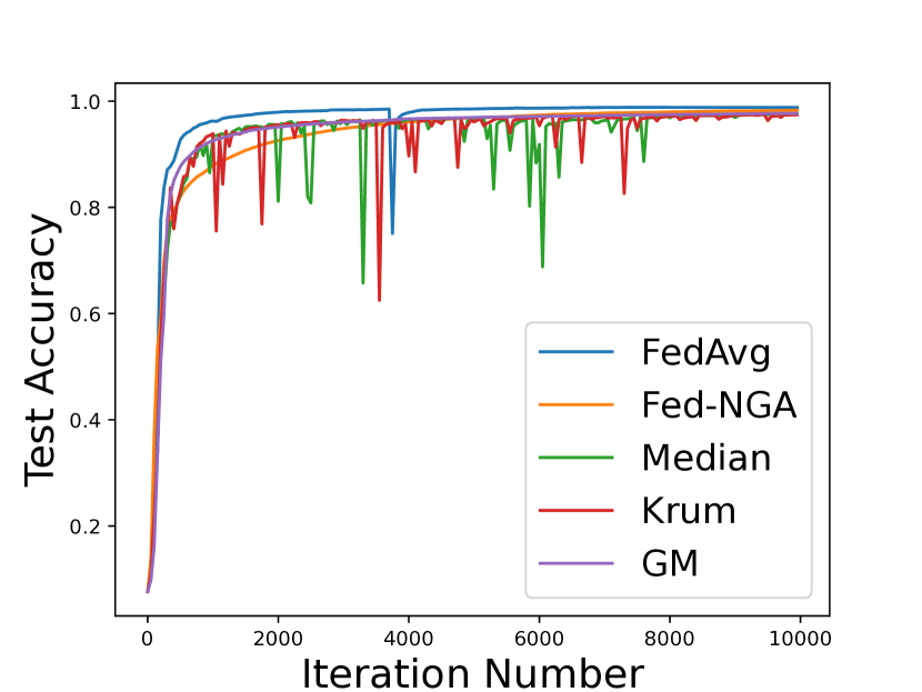
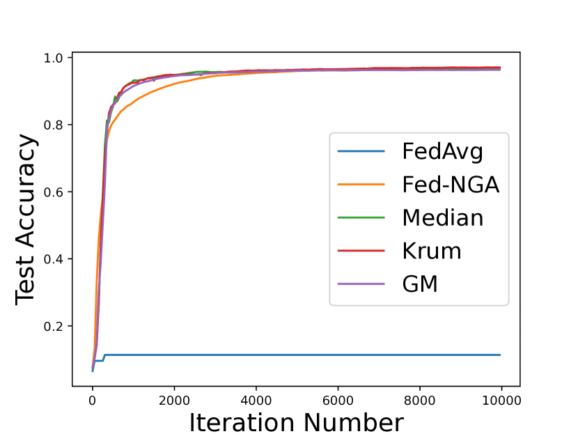
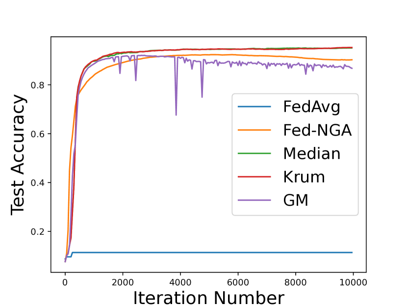
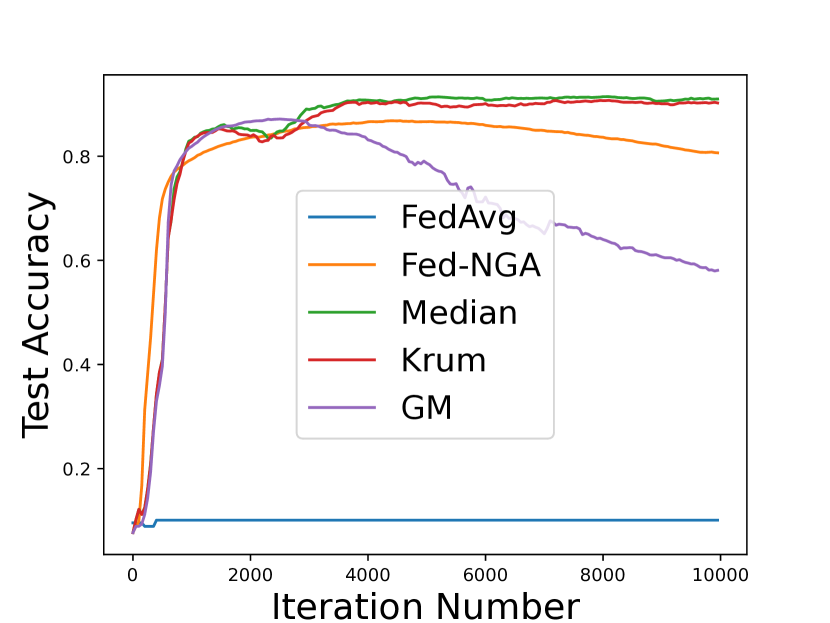
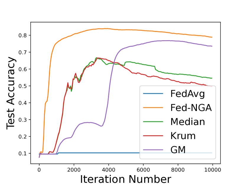
Figure 16: Test accuracy of LeNet with Same-value attacks for $\beta=0.4$. The intensity levels of Byzantine attack $\bar{C}_{\alpha}$ are 0, 0.1, 0.2, 0.3, 0.4 in order.

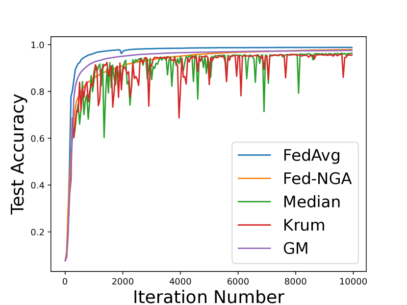
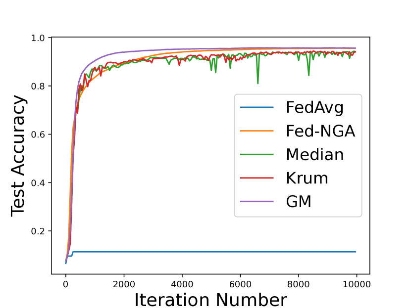
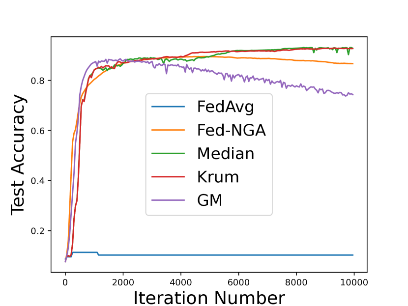
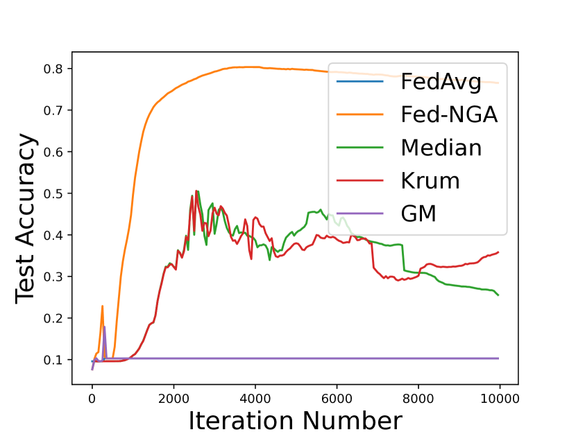
Figure 17: Test accuracy of LeNet with Same-value attacks for $\beta=0.2$. The intensity levels of Byzantine attack $\bar{C}_{\alpha}$ are 0, 0.1, 0.2, 0.3, 0.4 in order.

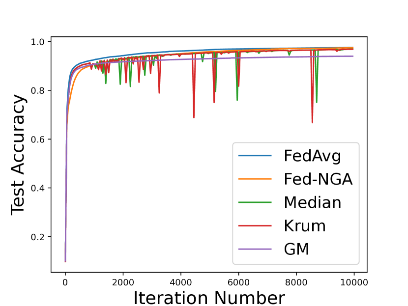
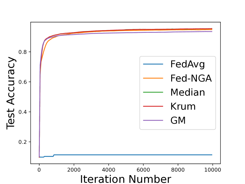
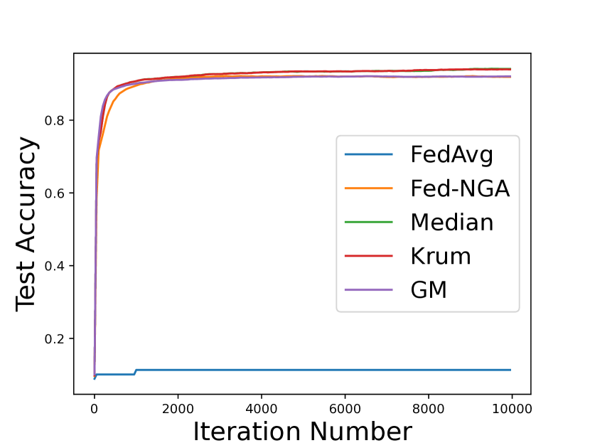
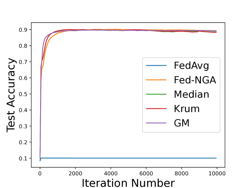
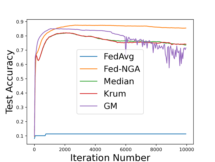
Figure 18: Test accuracy of MLP with Same-value attacks for $\beta=0.6$. The intensity levels of Byzantine attack $\bar{C}_{\alpha}$ are 0, 0.1, 0.2, 0.3, 0.4 in order.

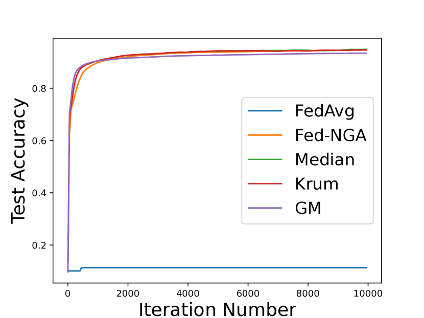
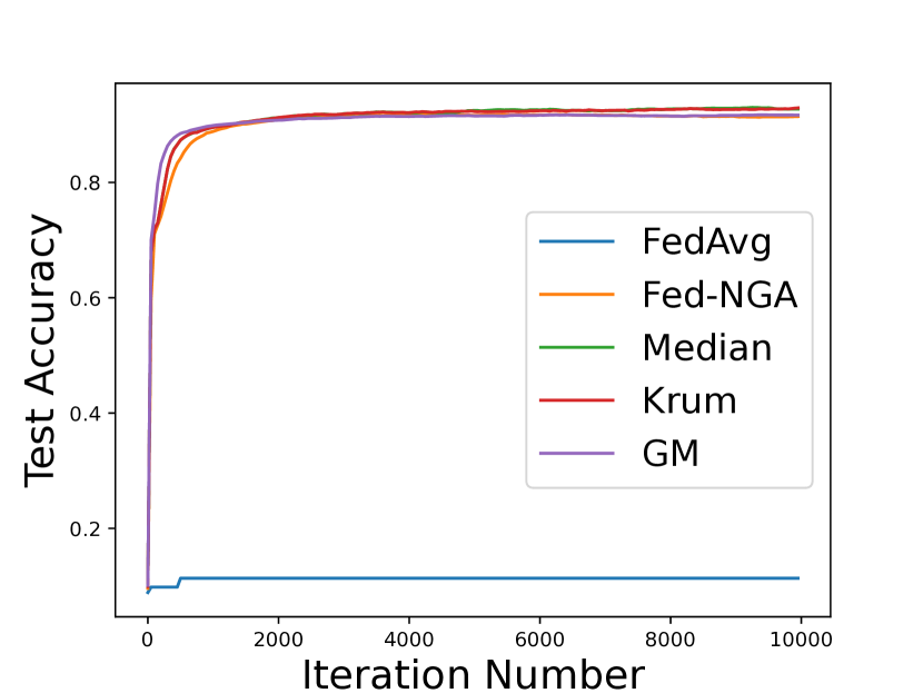
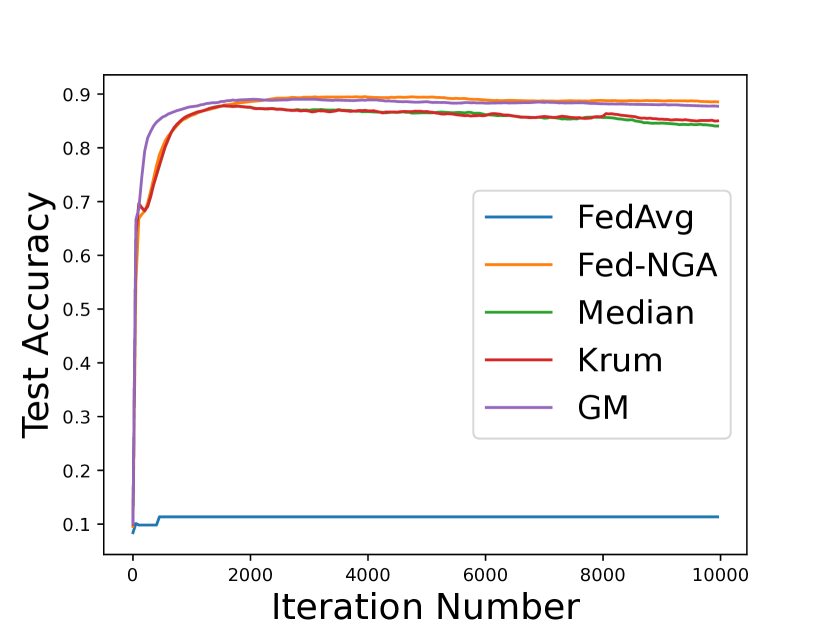
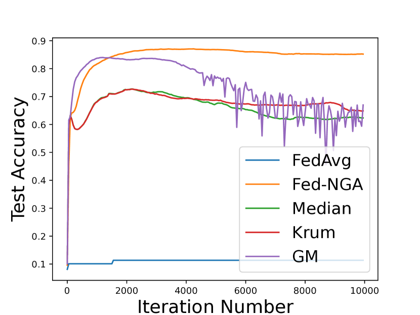
Figure 19: Test accuracy of MLP with Same-value attacks for $\beta=0.4$. The intensity levels of Byzantine attack $\bar{C}_{\alpha}$ are 0, 0.1, 0.2, 0.3, 0.4 in order.

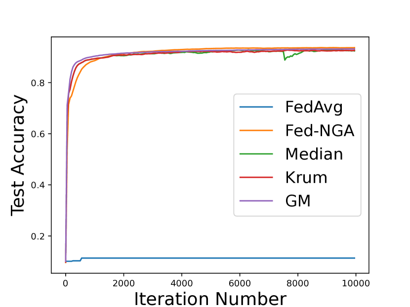
Figure 20: Test accuracy of MLP with Same-value attacks for $\beta=0.2$. The intensity levels of Byzantine attack $\bar{C}_{\alpha}$ are 0, 0.1, 0.2, 0.3, 0.4 in order.

Appendix D Related Works in Detail

FL is firstly proposed in (McMahan et al.,, 2017). The security issue in FL has been focused on since the emergence of FL (Vempaty et al.,, 2013; Yang et al.,, 2020). Byzantine attacks, as a common mean of distributed attacking, has also caught considerable research attention recently. In related works dealing with Byzantine attacks, various assumptions are made for loss function’s convexity (strongly convex or non-convex), and data heterogeneity (IID dataset or non-IID dataset). The valued achievement is to achieve zero optimality gap with rapid convergence. Furthermore, time complexity for aggregation is also a concerned performance metric as pointed out in Section 1. A detailed introduction of them is given in following subsections. Also a summary of these related works’ assumptions and performance is listed in Tab. 1.

D.1 Aggregation Strategy of Byzantine-resilient FL Algorithms

As of aggregation strategies in related literature, the measures to tolerate Byzantine attacks can be categorized as median, Krum, geometric median, etc. For the methods based on Median: Xie et al., (2018) takes the coordinate-wise median of the uploaded vectors as the aggregated one, while Yin et al., (2018) aggregates the upload vectors by calculating their coordinate-wise median or coordinate-wise trimmed mean. Differently, the Robust Aggregating Normalized Gradient Method (RANGE) (Turan et al.,, 2022) takes the median of uploaded vectors from each client as the aggregated one, and each uploaded vector is supposed to be the median of the local gradients from multiple steps of local updating. For the methods based on Krum: Blanchard et al., (2017) selects a stochastic gradient as the global one, which has the shortest Euclidean distance from a group of stochastic gradients that are most closely distributed with the total number of Byzantine clients given. For the methods based on Geometric median: all existing methods, including Robust Federated Aggregation (RFA) (Pillutla et al.,, 2022), Byzantine attack resilient distributed Stochastic Average Gradient Algorithm (Byrd-SAGA) (Wu et al.,, 2020), and Byzantine-RObust Aggregation with gradient Difference Compression And STochastic variance reduction (BROADCAST) (Zhu and Ling,, 2023), leverage the geometric median to aggregate upload vectors. Differently, RFA selects the tail-average of local model parameter over multiple local updating as the upload vector, both Byrd-SAGA and BROADCAST utilize the SAGA method (Defazio et al.,, 2014) to generate the upload message while the latter one allows uploading compressed message. For Other methods: Robust Stochastic Aggregation (RSA) (Li et al.,, 2019) penalizes the difference between local model parameters and global model parameters by $l_{d}$ norm to isolate Byzantine clients.

D.2 Assumptions and Performance of Byzantine-resilient FL Algorithms

For the methods based on Median: the aggregation complexity of median methods are all $\mathcal{O}(pM)$. To see the difference, Xie et al., (2018) verifies the robustness of Byzantine attacks on IID datasets only by experiments, while both trimmed mean (Yin et al.,, 2018) and RANGE (Turan et al.,, 2022) offer theoretical analysis for non-convex and strongly convex loss function on IID datasets. For the methods based on Krum: the aggregation complexity of Blanchard et al., (2017) is $\mathcal{O}(pM^{2})$ and convergence analysis is established on non-convex loss function and IID datasets. For the methods based on Geometric median: the time complexity for aggregation is $\mathcal{O}(pM\log^{3}(M\epsilon^{-1}))$ (Cohen et al.,, 2016) for all the three methods (Pillutla et al.,, 2022; Wu et al.,, 2020; Zhu and Ling,, 2023), which appear the robustness to Byzantine attacks under strongly convex loss function. Only RFA (Pillutla et al.,, 2022) reveals the proof on non-IID datasets, while both Byrd-SAGA (Wu et al.,, 2020) and BROADCAST (Zhu and Ling,, 2023) are established on IID datasets. For Other methods: The RSA (Li et al.,, 2019) has an aggregation complexity $\mathcal{O}({Mp^{3.5}})$. The convergence performance of RSA is analyzed on heterogeneous dataset for strongly convex loss function. Last but not least, the optimality gap of all the above algorithms are non-zero.

Different from the aforementioned works, we investigate both non-convex and strongly convex loss functions based on non-IID datasets, i.e., with the most generality to loss function type and dataset heterogeneity. Additionally, our proposed algorithm Fed-NGA only has a computation complexity $\mathcal{O}(pM)$, which is no larger than all the existing Byzantine robust algorithms. With such a low complexity, we can still achieve zero optimality gap, which cannot be realized by existing Byzantine robust algorithms either.

Appendix E Proof of Theorem 3.5

Under Assumption 3.1, and recalling (9) and (24), we have

$$F(w^{t+1})-F(w^{t}) \leqslant\left\langle\nabla F(w^{t}),w^{t+1}-w^{t}\right\rangle+\frac{L}{2}\left\lVert w^{t+1}-w^{t}\right\rVert^{2}$$ (25a)

$$=\eta^{t}\underbrace{\left\langle-\nabla F(w^{t}),g^{t}\right\rangle}_{A_{1}}+\frac{L}{2}(\eta^{t})^{2}\underbrace{\left\lVert g^{t}\right\rVert^{2}}_{A_{2}}.$$ (25b)

$A_{2}$ can be easily bounded because of Jensen’s inequality $f\left(\sum_{m\in\mathcal{M}}\alpha_{m}x_{m}\right)\leqslant\sum_{m\in\mathcal{M}}\alpha_{m}f(x_{m})$ with $\sum_{m\in\mathcal{M}}\alpha_{m}=1,\alpha_{m}>0$ for $m\in\mathcal{M}$ and $f(x)=x^{2}$, which implies that

$$A_{2} =\left\lVert g^{t}\right\rVert^{2}$$ (26a)

$$=\left\lVert\sum_{m\in\mathcal{M}}\alpha_{m}\cdot\frac{g_{m}^{t}}{\left\lVert g_{m}^{t}\right\rVert}\right\rVert^{2}$$ (26b)

$$\leqslant\sum_{m\in\mathcal{M}}\alpha_{m}\left\lVert\frac{g_{m}^{t}}{\left\lVert g_{m}^{t}\right\rVert}\right\rVert^{2}$$ (26c)

$$=1.$$ (26d)

Next, we aim to bound $A_{1}$. According to (24), there is

$$A_{1} =\left\langle-\nabla F(w^{t}),g^{t}\right\rangle$$ (27a)

$$=-\left\langle\nabla F(w)^{t},\sum_{m\in\mathcal{M}}\alpha_{m}\cdot\frac{g_{m}^{t}}{\left\lVert g_{m}^{t}\right\rVert}\right\rangle$$ (27b)

$$=-\sum_{m\in\mathcal{M}}\alpha_{m}\left\langle\nabla F(w^{t}),\frac{g_{m}^{t}}{\left\lVert g_{m}^{t}\right\rVert}\right\rangle$$ (27c)

$$=\underbrace{-\sum_{m\in\mathcal{M}\setminus\mathcal{B}}\alpha_{m}\left\langle\nabla F(w^{t}),\frac{g_{m}^{t}}{\left\lVert g_{m}^{t}\right\rVert}\right\rangle}_{B_{1}}+\left(\underbrace{-\sum_{m\in\mathcal{B}}\alpha_{m}\left\langle\nabla F(w^{t}),\frac{g_{m}^{t}}{\left\lVert g_{m}^{t}\right\rVert}\right\rangle}_{B_{2}}\right).$$ (27d)

$B_{2}$ is easier to be handled, so we first consider the bound of $B_{2}$. Because of $-\left\langle x,y\right\rangle\leqslant\left\lVert x\right\rVert\cdot\left\lVert y\right\rVert$, we have

$$B_{2} =-\sum_{m\in\mathcal{B}}\alpha_{m}\left\langle\nabla F(w^{t}),\frac{g_{m}^{t}}{\left\lVert g_{m}^{t}\right\rVert}\right\rangle$$ (28a)

$$\leqslant\sum_{m\in\mathcal{B}}\alpha_{m}\left\lVert\nabla F(w^{t})\right\rVert\cdot\left\lVert\frac{g_{m}^{t}}{\left\lVert g_{m}^{t}\right\rVert}\right\rVert$$ (28b)

$$\overset{\footnotesize{\tiny{1}⃝}}{=}\sum_{m\in\mathcal{B}}\alpha_{m}\left\lVert\nabla F(w^{t})\right\rVert$$ (28c)

$$\overset{\footnotesize{\tiny{2}⃝}}{=}(1-C_{\alpha})\left\lVert\nabla F(w^{t})\right\rVert,$$ (28d)

where \tiny{1}⃝ follows from $\displaystyle\left\lVert\frac{g_{m}^{t}}{\left\lVert g_{m}^{t}\right\rVert}\right\rVert=1$, and \tiny{2}⃝ comes from the definition of $C_{\alpha}$ in (7).

Then we aim to bound $B_{1}$, which implies that

$$B_{1} =-\sum_{m\in\mathcal{M}\setminus\mathcal{B}}\alpha_{m}\left\langle\nabla F(w^{t}),\frac{g_{m}^{t}}{\left\lVert g_{m}^{t}\right\rVert}\right\rangle$$ (29a)

$$=-\sum_{m\in\mathcal{M}\setminus\mathcal{B}}\alpha_{m}\left\langle\nabla F(w^{t}),\frac{\nabla F_{m}(w^{t})}{\left\lVert\nabla F_{m}(w^{t})\right\rVert}\right\rangle$$ (29b)

$$=-\sum_{m\in\mathcal{M}\setminus\mathcal{B}}\alpha_{m}\left(\left\langle\nabla F(w^{t}),\frac{\nabla F_{m}(w^{t})}{\left\lVert\nabla F_{m}(w^{t})\right\rVert}-\frac{\nabla F(w^{t})}{\left\lVert\nabla F(w^{t})\right\rVert}\right\rangle+\left\langle\nabla F(w^{t}),\frac{\nabla F(w^{t})}{\left\lVert\nabla F(w^{t})\right\rVert}\right\rangle\right)$$ (29c)

$$\overset{\footnotesize{\tiny{1}⃝}}{=}-\sum_{m\in\mathcal{M}\setminus\mathcal{B}}\alpha_{m}\left\langle\nabla F(w^{t}),\frac{\nabla F_{m}(w^{t})}{\left\lVert\nabla F_{m}(w^{t})\right\rVert}-\frac{\nabla F(w^{t})}{\left\lVert\nabla F(w^{t})\right\rVert}\right\rangle-C_{\alpha}\left\lVert\nabla F(w^{t})\right\rVert$$ (29d)

$$=\sum_{m\in\mathcal{M}\setminus\mathcal{B}}\alpha_{m}\left\lVert\nabla F(w^{t})\right\rVert\left\langle\frac{\nabla F(w^{t})}{\left\lVert\nabla F(w^{t})\right\rVert},\frac{\nabla F(w^{t})}{\left\lVert\nabla F(w^{t})\right\rVert}-\frac{\nabla F_{m}(w^{t})}{\left\lVert\nabla F_{m}(w^{t})\right\rVert}\right\rangle-C_{\alpha}\left\lVert\nabla F(w^{t})\right\rVert$$ (29e)

$$\overset{\footnotesize{\tiny{2}⃝}}{=}\sum_{m\in\mathcal{M}\setminus\mathcal{B}}\frac{\alpha_{m}\left\lVert\nabla F(w^{t})\right\rVert}{2}\left(\left\lVert\frac{\nabla F(w^{t})}{\left\lVert\nabla F(w^{t})\right\rVert}\right\rVert^{2}+\left\lVert\frac{\nabla F_{m}(w^{t})}{\left\lVert\nabla F_{m}(w^{t})\right\rVert}-\frac{\nabla F(w^{t})}{\left\lVert\nabla F(w^{t})\right\rVert}\right\rVert^{2}-\left\lVert\frac{\nabla F_{m}(w^{t})}{\left\lVert\nabla F_{m}(w^{t})\right\rVert}\right\rVert^{2}\right)$$

$$\quad-C_{\alpha}\left\lVert\nabla F(w^{t})\right\rVert$$ (29f)

$$=\sum_{m\in\mathcal{M}\setminus\mathcal{B}}\frac{\alpha_{m}\left\lVert\nabla F(w^{t})\right\rVert}{2}\left(1+(\theta_{m}^{t})^{2}-1\right)-C_{\alpha}\left\lVert\nabla F(w^{t})\right\rVert$$ (29g)

$$\overset{\footnotesize{\tiny{3}⃝}}{\leqslant}\frac{1}{2}C_{\alpha}(\theta)^{2}\left\lVert\nabla F(w^{t})\right\rVert-C_{\alpha}\left\lVert\nabla F(w^{t})\right\rVert$$ (29h)

$$=-\left(1-\frac{(\theta)^{2}}{2}\right)\cdot C_{\alpha}\left\lVert\nabla F(w^{t})\right\rVert,$$ (29i)

where

• \tiny{1}⃝ holds because $\left\langle x,x\right\rangle=\left\lVert x\right\rVert^{2}$ and the definition of $C_{\alpha}$ in (7).

• \tiny{2}⃝ can be derived from $\left\langle x,y\right\rangle=\frac{1}{2}\left\lVert x\right\rVert^{2}+\frac{1}{2}\left\lVert y\right\rVert^{2}-\frac{1}{2}\left\lVert x-y\right\rVert^{2}$.

• \tiny{3}⃝ is bounded by Assumption 3.4.

Combining (28) and (29), we have

$$A_{1} =B_{1}+B_{2}$$ (30a)

$$\leqslant-(1-\frac{(\theta)^{2}}{2})\cdot C_{\alpha}\left\lVert\nabla F(w^{t})\right\rVert+(1-C_{\alpha})\left\lVert\nabla F(w^{t})\right\rVert$$ (30b)

$$=-\left(\left(2-\frac{(\theta)^{2}}{2}\right)C_{\alpha}-1\right)\left\lVert\nabla F(w^{t})\right\rVert.$$ (30c)

Then combining $A_{1}$ in (30) and $A_{2}$ in (26), there is

$$F(w^{t+1})-F(w^{t}) \leqslant\eta^{t}\cdot A_{1}+\frac{L}{2}(\eta^{t})^{2}\cdot A_{2}$$ (31a)

$$\leqslant-\eta^{t}\left(\left(2-\frac{(\theta)^{2}}{2}\right)C_{\alpha}-1\right)\left\lVert\nabla F(w^{t})\right\rVert+\frac{L}{2}(\eta^{t})^{2}.$$ (31b)

Summing up the inequality in (31) for $t=0,1,\cdots,T-1$, we obtain

$$F(w^{T})-F(w^{0})\leqslant-\left(\left(2-\frac{(\theta)^{2}}{2}\right)C_{\alpha}-1\right)\sum_{t=0}^{T-1}\eta^{t}\left\lVert\nabla F(w^{t})\right\rVert+\frac{L}{2}\sum_{t=0}^{T-1}(\eta^{t})^{2},$$ (32)

When $\displaystyle\left(2-\frac{(\theta)^{2}}{2}\right)C_{\alpha}-1>0$, dividing the inequality in (32) by $\displaystyle\left(\left(2-\frac{(\theta)^{2}}{2}\right)C_{\alpha}-1\right)\sum_{t=0}^{T-1}\eta^{t}$ on both sides, we have

$$\qquad\frac{1}{\sum_{t=0}^{T-1}\eta^{t}}\sum_{t=0}^{T-1}\eta^{t}\left\lVert\nabla F(w^{t})\right\rVert$$

$$\leqslant\frac{F(w^{0})-F(w^{T})}{\left((2-\frac{(\theta)^{2}}{2})C_{\alpha}-1\right)\sum_{t=0}^{T-1}\eta^{t}}+\frac{L\sum_{t=0}^{T-1}(\eta^{t})^{2}}{2\left((2-\frac{(\theta)^{2}}{2})C_{\alpha}-1\right)\sum_{t=0}^{T-1}\eta^{t}}.$$ (33)

This completes the proof of Theorem 3.5.

Appendix F Proof of Theorem 3.7

The proof of inequalities (20) and (21) are both based on Lemma F.1.

Lemma F.1.

With Assumption 3.1, Assumption 3.2, Assumption 3.3 and Assumption 3.4, when $\gamma>0$, $\left\lVert w^{t+1}-w^{*}\right\rVert^{2}$ can be bounded as follows

$$\left\lVert w^{t+1}-w^{*}\right\rVert^{2}\leqslant\left(1-\gamma\cdot\eta^{t}\right)\left\lVert w^{t}-w^{*}\right\rVert^{2}+(\eta^{t})^{2},$$ (34)

where $\gamma=2((\mu+L-L\cdot\theta)C_{\alpha}-L)/G$.

Proof.

Please refer to Appendix G. ∎

F.1 Proof of Convergence Result in (20)

Applying the inequality in Lemma F.1 for $t=0,1,\cdots,T-1$, when $\displaystyle\eta^{t}<\frac{1}{\gamma}$ for $t=0,1,\cdots,T-1$, we then have

$$\left\lVert w^{T}-w^{*}\right\rVert^{2}\leqslant\prod_{t=0}^{T-1}(1-\gamma\cdot\eta^{t})\left\lVert w^{0}-w^{*}\right\rVert^{2}+\sum_{t=0}^{T-2}(\eta^{t})^{2}\prod_{i=t+1}^{T-1}(1-\gamma\cdot\eta^{i})+(\eta^{T-1})^{2}.$$ (35)

This completes the proof of convergence result in (20).

F.2 Proof of Convergence Result in (21)

Summarizing the inequality in Lemma F.1 for $t=0,1,\cdots,T-1$, we obtain that

$$\sum_{t=1}^{T}\left\lVert w^{t}-w^{*}\right\rVert^{2}\leqslant\sum_{t=0}^{T-1}\left(1-\gamma\cdot\eta^{t}\right)\left\lVert w^{t}-w^{*}\right\rVert^{2}+\sum_{t=0}^{T-1}(\eta^{t})^{2}.$$ (36)

After merging similar items, there is

$$\left\lVert w^{T}-w^{*}\right\rVert^{2}+\sum_{t=0}^{T-1}\gamma\cdot\eta^{t}\left\lVert w^{t}-w^{*}\right\rVert^{2}\leqslant\left\lVert w^{0}-w^{*}\right\rVert^{2}+\sum_{t=0}^{T-1}(\eta^{t})^{2},$$ (37)

When $\displaystyle\eta^{T}<\frac{1}{\gamma}$, there is

$$\sum_{t=0}^{T}\gamma\cdot\eta^{t}\left\lVert w^{t}-w^{*}\right\rVert^{2}\leqslant\left\lVert w^{T}-w^{*}\right\rVert^{2}+\sum_{t=0}^{T-1}\gamma\cdot\eta^{t}\left\lVert w^{t}-w^{*}\right\rVert^{2}.$$ (38)

Combining the inequalities in (37) and (38), we have

$$\sum_{t=0}^{T}\gamma\cdot\eta^{t}\left\lVert w^{t}-w^{*}\right\rVert^{2}\leqslant\left\lVert w^{0}-w^{*}\right\rVert^{2}+\sum_{t=0}^{T-1}(\eta^{t})^{2}.$$ (39)

Dividing the inequality in (39) by $\gamma\cdot\sum_{t=0}^{T}\eta^{t}$ for both sizes, we further have

$$\frac{1}{\sum_{t=0}^{T}\eta^{t}}\sum_{t=0}^{T}\eta^{t}\left\lVert w^{t}-w^{*}\right\rVert^{2}\leqslant\frac{\left\lVert w^{0}-w^{*}\right\rVert^{2}}{\gamma\sum_{t=0}^{T}\eta^{t}}+\frac{\sum_{t=0}^{T-1}(\eta^{t})^{2}}{\gamma\sum_{t=0}^{T}\eta^{t}}.$$ (40)

This completes the proof of the convergence result in (21).

Appendix G Proof of Lemma F.1

In this section, we aim to bound $\left\lVert w^{t+1}-w^{*}\right\rVert^{2}$. There is

$$\left\lVert w^{t+1}-w^{*}\right\rVert^{2} =\left\lVert w^{t}-\eta^{t}\cdot g^{t}-w^{*}\right\rVert^{2}$$ (41a)

$$=\left\lVert w^{t}-w^{*}\right\rVert^{2}+(\eta^{t})^{2}\underbrace{\left\lVert g^{t}\right\rVert^{2}}_{A_{2}}+2\eta^{t}\underbrace{-\left\langle w^{t}-w^{*},g^{t}\right\rangle}_{C_{1}}.$$ (41b)

Thanks to the inequality in (26), we obtain that

$$A_{2} =\left\lVert g^{t}\right\rVert^{2}$$

$$\leqslant 1.$$ (42)

Then we aim to bound $C_{1}$. We have

$$C_{1} =-\left\langle w^{t}-w^{*},g^{t}\right\rangle$$ (43a)

$$=-\left\langle w^{t}-w^{*},\sum_{m\in\mathcal{M}}\alpha_{m}\cdot\frac{g_{m}^{t}}{\left\lVert g_{m}^{t}\right\rVert}\right\rangle$$ (43b)

$$=-\sum_{m\in\mathcal{M}}\alpha_{m}\left\langle w^{t}-w^{*},\frac{g_{m}^{t}}{\left\lVert g_{m}^{t}\right\rVert}\right\rangle$$ (43c)

$$=\underbrace{-\sum_{m\in\mathcal{M}\setminus\mathcal{B}}\alpha_{m}\left\langle w^{t}-w^{*},\frac{g_{m}^{t}}{\left\lVert g_{m}^{t}\right\rVert}\right\rangle}_{D_{1}}+\left(\underbrace{-\sum_{m\in\mathcal{B}}\alpha_{m}\left\langle w^{t}-w^{*},\frac{g_{m}^{t}}{\left\lVert g_{m}^{t}\right\rVert}\right\rangle}_{D_{2}}\right).$$ (43d)

$D_{2}$ is easier to be bounded, so we first consider the bound of $D_{2}$. Because $-\left\langle x,y\right\rangle\leqslant\left\lVert x\right\rVert\cdot\left\lVert y\right\rVert$, we obtain

$$D_{2} =-\sum_{m\in\mathcal{B}}\alpha_{m}\left\langle w^{t}-w^{*},\frac{g_{m}^{t}}{\left\lVert g_{m}^{t}\right\rVert}\right\rangle$$ (44a)

$$\leqslant\sum_{m\in\mathcal{B}}\alpha_{m}\left\lVert w^{t}-w^{*}\right\rVert\cdot\left\lVert\frac{g_{m}^{t}}{\left\lVert g_{m}^{t}\right\rVert}\right\rVert$$ (44b)

$$\overset{\footnotesize{\tiny{1}⃝}}{=}\sum_{m\in\mathcal{B}}\alpha_{m}\left\lVert w^{t}-w^{*}\right\rVert$$ (44c)

$$\overset{\footnotesize{\tiny{2}⃝}}{=}(1-C_{\alpha})\left\lVert w^{t}-w^{*}\right\rVert,$$ (44d)

where \tiny{1}⃝ is established by $\displaystyle\left\lVert\frac{g_{m}^{t}}{\left\lVert g_{m}^{t}\right\rVert}\right\rVert=1$ and \tiny{2}⃝ comes from the definition of $C_{\alpha}$ in (7).

Then we switch to bound$D_{1}$. It follows that

$$D_{1} =-\sum_{m\in\mathcal{M}\setminus\mathcal{B}}\alpha_{m}\left\langle w^{t}-w^{*},\frac{g_{m}^{t}}{\left\lVert g_{m}^{t}\right\rVert}\right\rangle$$ (45a)

$$=-\sum_{m\in\mathcal{M}\setminus\mathcal{B}}\alpha_{m}\left\langle w^{t}-w^{*},\frac{\nabla F_{m}(w^{t})}{\left\lVert\nabla F_{m}(w^{t})\right\rVert}\right\rangle$$ (45b)

$$=\underbrace{-\sum_{m\in\mathcal{M}\setminus\mathcal{B}}\alpha_{m}\left\langle w^{t}-w^{*},\frac{\nabla F_{m}(w^{t})}{\left\lVert\nabla F_{m}(w^{t})\right\rVert}-\frac{\nabla F(w^{t})}{\left\lVert\nabla F(w^{t})\right\rVert}\right\rangle}_{E_{1}}+\left(\underbrace{-\sum_{m\in\mathcal{M}\setminus\mathcal{B}}\alpha_{m}\left\langle w^{t}-w^{*},\frac{\nabla F(w^{t})}{\left\lVert\nabla F(w^{t})\right\rVert}\right\rangle}_{E_{2}}\right).$$ (45c)

$E_{1}$ can be bounded by $-\left\langle x,y\right\rangle\leqslant\left\lVert x\right\rVert\cdot\left\lVert y\right\rVert$ and Assumption 3.4, which implies that

$$E_{1} =-\sum_{m\in\mathcal{M}\setminus\mathcal{B}}\alpha_{m}\left\langle w^{t}-w^{*},\frac{\nabla F_{m}(w^{t})}{\left\lVert\nabla F_{m}(w^{t})\right\rVert}-\frac{\nabla F(w^{t})}{\left\lVert\nabla F(w^{t})\right\rVert}\right\rangle$$ (46a)

$$\leqslant\sum_{m\in\mathcal{M}\setminus\mathcal{B}}\alpha_{m}\left\lVert w^{t}-w^{*}\right\rVert\cdot\left\lVert\frac{\nabla F_{m}(w^{t})}{\left\lVert\nabla F_{m}(w^{t})\right\rVert}-\frac{\nabla F(w^{t})}{\left\lVert\nabla F(w^{t})\right\rVert}\right\rVert$$ (46b)

$$=\sum_{m\in\mathcal{M}\setminus\mathcal{B}}\alpha_{m}\left\lVert w^{t}-w^{*}\right\rVert\cdot\theta_{m}^{t}$$ (46c)

$$\leqslant C_{\alpha}\theta\left\lVert w^{t}-w^{*}\right\rVert.$$ (46d)

For $E_{2}$, with Assumption 3.2 and $\nabla F(w^{*})=0$, there is

$$E_{2} =-\sum_{m\in\mathcal{M}\setminus\mathcal{B}}\alpha_{m}\left\langle w^{t}-w^{*},\frac{\nabla F(w^{t})}{\left\lVert\nabla F(w^{t})\right\rVert}\right\rangle$$ (47a)

$$=-\sum_{m\in\mathcal{M}\setminus\mathcal{B}}\alpha_{m}\left\langle w^{t}-w^{*},\frac{\nabla F(w^{t})-\nabla F(w^{*})}{\left\lVert\nabla F(w^{t})\right\rVert}\right\rangle$$ (47b)

$$\leqslant-\sum_{m\in\mathcal{M}\setminus\mathcal{B}}\mu\alpha_{m}\frac{\left\lVert w^{t}-w^{*}\right\rVert^{2}}{\left\lVert\nabla F(w^{t})\right\rVert}$$ (47c)

$$=-\mu C_{\alpha}\frac{\left\lVert w^{t}-w^{*}\right\rVert^{2}}{\left\lVert\nabla F(w^{t})\right\rVert}.$$ (47d)

Combining $E_{1}$ in (46) and $E_{2}$ in (47), we obtain

$$D_{1} =E_{1}+E_{2}$$

$$\leqslant-\mu C_{\alpha}\frac{\left\lVert w^{t}-w^{*}\right\rVert^{2}}{\left\lVert\nabla F(w^{t})\right\rVert}+C_{\alpha}\theta\left\lVert w^{t}-w^{*}\right\rVert.$$ (48)

Then combining $D_{1}$ in (G) and $D_{2}$ in (44), for $(\mu+L-L\cdot\theta)C_{\alpha}-L>0$, we have

$$C_{1} =D_{1}+D_{2}$$ (49a)

$$\leqslant-\mu C_{\alpha}\frac{\left\lVert w^{t}-w^{*}\right\rVert^{2}}{\left\lVert\nabla F(w^{t})\right\rVert}+C_{\alpha}\theta\left\lVert w^{t}-w^{*}\right\rVert+(1-C_{\alpha})\left\lVert w^{t}-w^{*}\right\rVert$$ (49b)

$$=-\mu C_{\alpha}\frac{\left\lVert w^{t}-w^{*}\right\rVert^{2}}{\left\lVert\nabla F(w^{t})\right\rVert}+C_{\alpha}\theta\frac{\left\lVert w^{t}-w^{*}\right\rVert^{2}}{\left\lVert w^{t}-w^{*}\right\rVert}+(1-C_{\alpha})\frac{\left\lVert w^{t}-w^{*}\right\rVert^{2}}{\left\lVert w^{t}-w^{*}\right\rVert}$$ (49c)

$$\overset{\footnotesize{\tiny{1}⃝}}{\leqslant}-\mu C_{\alpha}\frac{\left\lVert w^{t}-w^{*}\right\rVert^{2}}{\left\lVert\nabla F(w^{t})\right\rVert}+C_{\alpha}\theta L\frac{\left\lVert w^{t}-w^{*}\right\rVert^{2}}{\left\lVert\nabla F(w^{t})-\nabla F(w^{*})\right\rVert}+(1-C_{\alpha})L\frac{\left\lVert w^{t}-w^{*}\right\rVert^{2}}{\left\lVert\nabla F(w^{t})-\nabla F(w^{*})\right\rVert}$$ (49d)

$$\overset{\footnotesize{\tiny{2}⃝}}{=}-\mu C_{\alpha}\frac{\left\lVert w^{t}-w^{*}\right\rVert^{2}}{\left\lVert\nabla F(w^{t})\right\rVert}+C_{\alpha}\theta L\frac{\left\lVert w^{t}-w^{*}\right\rVert^{2}}{\left\lVert\nabla F(w^{t})\right\rVert}+(1-C_{\alpha})L\frac{\left\lVert w^{t}-w^{*}\right\rVert^{2}}{\left\lVert\nabla F(w^{t})\right\rVert}$$ (49e)

$$=-\left((\mu+L-L\cdot\theta)C_{\alpha}-L\right)\frac{\left\lVert w^{t}-w^{*}\right\rVert^{2}}{\left\lVert\nabla F(w^{t})\right\rVert}$$ (49f)

$$\overset{\footnotesize{\tiny{3}⃝}}{\leqslant}-\frac{(\mu+L-L\cdot\theta)C_{\alpha}-L}{G}\left\lVert w^{t}-w^{*}\right\rVert^{2},$$ (49g)

where

• \tiny{1}⃝ comes from Assumption 3.1.

• \tiny{2}⃝ is established because $\nabla F(w^{*})=0$.

• \tiny{3}⃝ can be derived by Assumption 3.3.

Based on (41), combining $A_{2}$ in (26) and $C_{1}$ in (49), there is

$$\left\lVert w^{t+1}-w^{*}\right\rVert^{2} =\left\lVert w^{t}-w^{*}\right\rVert^{2}+(\eta^{t})^{2}\cdot A_{2}+2\eta^{t}\cdot C_{1}$$

$$\leqslant\left(1-2\eta^{t}\frac{(\mu+L-L\cdot\theta)C_{\alpha}-L}{G}\right)\left\lVert w^{t}-w^{*}\right\rVert^{2}+(\eta^{t})^{2}.$$ (50)

We denote $\gamma=2((\mu+L-L\cdot\theta)C_{\alpha}-L)/G$, which implies that

$$\left\lVert w^{t+1}-w^{*}\right\rVert^{2}\leqslant\left(1-\gamma\cdot\eta^{t}\right)\left\lVert w^{t}-w^{*}\right\rVert^{2}+(\eta^{t})^{2}.$$ (51)

This completes the proof of Lemma F.1.

References

- Blanchard et al., (2017) Blanchard, P., El Mhamdi, E. M., Guerraoui, R., and Stainer, J. (2017). Machine learning with adversaries: Byzantine tolerant gradient descent. Advances in neural information processing systems, 30.
- Cao and Lai, (2019) Cao, X. and Lai, L. (2019). Distributed gradient descent algorithm robust to an arbitrary number of byzantine attackers. IEEE Transactions on Signal Processing, 67(22):5850–5864.
- Chen et al., (2017) Chen, Y., Su, L., and Xu, J. (2017). Distributed statistical machine learning in adversarial settings: Byzantine gradient descent. Proceedings of the ACM on Measurement and Analysis of Computing Systems, 1(2):1–25.
- Cohen et al., (2016) Cohen, M. B., Lee, Y. T., Miller, G., Pachocki, J., and Sidford, A. (2016). Geometric median in nearly linear time. In Proceedings of the forty-eighth annual ACM symposium on Theory of Computing, pages 9–21.
- Defazio et al., (2014) Defazio, A., Bach, F., and Lacoste-Julien, S. (2014). Saga: A fast incremental gradient method with support for non-strongly convex composite objectives. Advances in neural information processing systems, 27.
- Dorfman et al., (2023) Dorfman, R., Vargaftik, S., Ben-Itzhak, Y., and Levy, K. Y. (2023). Docofl: downlink compression for cross-device federated learning. In International Conference on Machine Learning, pages 8356–8388. PMLR.
- Guo et al., (2023) Guo, Y., Tang, X., and Lin, T. (2023). Fedbr: Improving federated learning on heterogeneous data via local learning bias reduction. In International Conference on Machine Learning, pages 12034–12054. PMLR.
- Huang et al., (2023) Huang, M., Zhang, D., and Ji, K. (2023). Achieving linear speedup in non-iid federated bilevel learning. In International Conference on Machine Learning, pages 14039–14059. PMLR.
- Kairouz et al., (2021) Kairouz, P., McMahan, H. B., Avent, B., Bellet, A., Bennis, M., Bhagoji, A. N., Bonawitz, K., Charles, Z., Cormode, G., Cummings, R., et al. (2021). Advances and open problems in federated learning. Foundations and trends® in machine learning, 14(1–2):1–210.
- Konečnỳ et al., (2016) Konečnỳ, J., McMahan, H. B., Yu, F. X., Richtárik, P., Suresh, A. T., and Bacon, D. (2016). Federated learning: Strategies for improving communication efficiency. arXiv preprint arXiv:1610.05492.
- LeCun et al., (1998) LeCun, Y., Bottou, L., Bengio, Y., and Haffner, P. (1998). Gradient-based learning applied to document recognition. Proceedings of the IEEE, 86(11):2278–2324.
- Li et al., (2019) Li, L., Xu, W., Chen, T., Giannakis, G. B., and Ling, Q. (2019). RSA: Byzantine-robust stochastic aggregation methods for distributed learning from heterogeneous datasets. In Proceedings of the AAAI conference on artificial intelligence, volume 33, pages 1544–1551.
- Li et al., (2020) Li, T., Sahu, A. K., Zaheer, M., Sanjabi, M., Talwalkar, A., and Smith, V. (2020). Federated optimization in heterogeneous networks. Proceedings of Machine learning and systems, 2:429–450.
- Li and Li, (2023) Li, X. and Li, P. (2023). Analysis of error feedback in federated non-convex optimization with biased compression: Fast convergence and partial participation. In International Conference on Machine Learning, pages 19638–19688. PMLR.
- McMahan et al., (2017) McMahan, B., Moore, E., Ramage, D., Hampson, S., and y Arcas, B. A. (2017). Communication-efficient learning of deep networks from decentralized data. In Artificial intelligence and statistics, pages 1273–1282. PMLR.
- Pillutla et al., (2022) Pillutla, K., Kakade, S. M., and Harchaoui, Z. (2022). Robust aggregation for federated learning. IEEE Transactions on Signal Processing, 70:1142–1154.
- So et al., (2020) So, J., Güler, B., and Avestimehr, A. S. (2020). Byzantine-resilient secure federated learning. IEEE Journal on Selected Areas in Communications, 39(7):2168–2181.
- Turan et al., (2022) Turan, B., Uribe, C. A., Wai, H.-T., and Alizadeh, M. (2022). Robust distributed optimization with randomly corrupted gradients. IEEE Transactions on Signal Processing, 70:3484–3498.
- Vempaty et al., (2013) Vempaty, A., Tong, L., and Varshney, P. K. (2013). Distributed inference with byzantine data: State-of-the-art review on data falsification attacks. IEEE Signal Processing Magazine, 30(5):65–75.
- Wang et al., (2019) Wang, S., Tuor, T., Salonidis, T., Leung, K. K., Makaya, C., He, T., and Chan, K. (2019). Adaptive federated learning in resource constrained edge computing systems. IEEE journal on selected areas in communications, 37(6):1205–1221.
- Wu et al., (2023) Wu, F., Guo, S., Qu, Z., He, S., Liu, Z., and Gao, J. (2023). Anchor sampling for federated learning with partial client participation. In International Conference on Machine Learning, pages 37379–37416. PMLR.
- Wu et al., (2020) Wu, Z., Ling, Q., Chen, T., and Giannakis, G. B. (2020). Federated variance-reduced stochastic gradient descent with robustness to byzantine attacks. IEEE Transactions on Signal Processing, 68:4583–4596.
- Xiao and Ji, (2023) Xiao, P. and Ji, K. (2023). Communication-efficient federated hypergradient computation via aggregated iterative differentiation. In International Conference on Machine Learning, pages 38059–38086. PMLR.
- Xie et al., (2018) Xie, C., Koyejo, O., and Gupta, I. (2018). Generalized byzantine-tolerant SGD. arXiv preprint arXiv:1802.10116.
- Xie and Song, (2023) Xie, Z. and Song, S. (2023). Fedkl: Tackling data heterogeneity in federated reinforcement learning by penalizing kl divergence. IEEE Journal on Selected Areas in Communications, 41(4):1227–1242.
- Yang et al., (2020) Yang, Z., Gang, A., and Bajwa, W. U. (2020). Adversary-resilient distributed and decentralized statistical inference and machine learning: An overview of recent advances under the byzantine threat model. IEEE Signal Processing Magazine, 37(3):146–159.
- Yin et al., (2018) Yin, D., Chen, Y., Kannan, R., and Bartlett, P. (2018). Byzantine-robust distributed learning: Towards optimal statistical rates. In International Conference on Machine Learning, pages 5650–5659. PMLR.
- Yue et al., (2022) Yue, K., Jin, R., Pilgrim, R., Wong, C.-W., Baron, D., and Dai, H. (2022). Neural tangent kernel empowered federated learning. In International Conference on Machine Learning, pages 25783–25803. PMLR.
- Zhao et al., (2024) Zhao, P., Yu, F., and Wan, Z. (2024). A huber loss minimization approach to byzantine robust federated learning. In Proceedings of the AAAI Conference on Artificial Intelligence, volume 38, pages 21806–21814.
- Zhao et al., (2018) Zhao, Y., Li, M., Lai, L., Suda, N., Civin, D., and Chandra, V. (2018). Federated learning with non-iid data. arXiv preprint arXiv:1806.00582.
- Zhu and Ling, (2023) Zhu, H. and Ling, Q. (2023). Byzantine-robust distributed learning with compression. IEEE Transactions on Signal and Information Processing over Networks.
- Zuo et al., (2024) Zuo, S., Yan, X., Fan, R., Hu, H., Shan, H., and Quek, T. Q. S. (2024). Byzantine-resilient federated learning with adaptivity to data heterogeneity.