Sample-Optimal Large-Scale Optimal Subset Selection

Sample-Optimal Large-Scale Optimal Subset Selection

Zaile Li Technology and Operations Management Area, INSEAD, Fontainebleau, France
zaile.li@insead.edu Weiwei Fan Advanced Institute of Business and School of Economics and Management, Tongji University, Shanghai, China wfan@tongji.edu.cn L. Jeff Hong School of Management and School of Data Science, Fudan University, Shanghai, China
hong_liu@fudan.edu.cn

Ranking and selection (R&S) conventionally aims to select the unique best alternative with the largest mean performance from a finite set of alternatives. However, for better supporting decision making, it may be more informative to deliver a small menu of alternatives whose mean performances are among the top $m$. Such problem, called optimal subset selection (OSS), is generally more challenging to address than the conventional R&S. This challenge becomes even more significant when the number of alternatives is considerably large. Thus, the focus of this paper is on addressing the large-scale OSS problem. To achieve this goal, we design a top-$m$ greedy selection mechanism that keeps sampling the current top $m$ alternatives with top $m$ running sample means and propose the explore-first top-$m$ greedy (EFG-$m$) procedure. Through an extended boundary-crossing framework, we prove that the EFG-$m$ procedure is both sample optimal and consistent in terms of the probability of good selection, confirming its effectiveness in solving large-scale OSS problem. Surprisingly, we also demonstrate that the EFG-$m$ procedure enables to achieve an indifference-based ranking within the selected subset of alternatives at no extra cost. This is highly beneficial as it delivers deeper insights to decision-makers, enabling more informed decision-makings. Lastly, numerical experiments validate our results and demonstrate the efficiency of our procedures.

optimal subset selection, large-scale, greedy, sample optimality, ranking, boundary-crossing

1 Introduction

Practical decision-making often involves comparing and selecting among a finite number of alternatives within a complex stochastic environment. These alternatives may refer to intervention strategies for an influenza pandemic (Paleshi et al. 2017), emergency evacuation plans during disasters (Zhang et al. 2023), and choices of hyper-parameters in algorithm training (Luo et al. 2022). Simulation has become as a prevalent tool in these scenarios, due to its capability to sample and estimate the performance of each alternative. Conventionally, the objective of such simulation-based decision-making is to optimize across all alternatives to select the best alternative, which is defined to have the largest (or smallest) mean performance. This formulation is known as ranking and selection (R&S) and has been widely studied in simulation community. When the sampling budget is limited, the effectiveness of a R&S procedure is often measured by the resulting probability of correct selection/good selection (PCS/PGS). Interested readers are encouraged to refer to Kim and Nelson (2006), Chen and Lee (2011) and Hong et al. (2021) for comprehensive reviews of these procedures.

However, the R&S formulation of only selecting the best alternative may not always be suitable in practice. In many scenarios, decision makers need to consider multiple factors like economic implications, regulatory constraints, or qualitative evaluations before finalizing their decision (Monks and Currie 2018, Eckman et al. 2020). A case in point is Cornell University’s strategy during the COVID-19 pandemic, which required simultaneous consideration of residential infections and testing frequency (Frazier et al. 2022). To address this problem, the university’s simulation team initially identified the top-6 testing policies that can effectively minimize residential infections. After this initial selection, they then recommended the most efficient one in terms of testing frequency. This approach, which involves selecting not just the single best but a subset of top $m$ alternatives, is known as optimal subset selection (OSS) or top-$m$ selection (Koenig and Law 1985, Chen et al. 2008, Gao and Chen 2015, 2016, Zhang et al. 2023). The OSS formulation is particularly advantageous because it allows decision-makers to perform a comprehensive evaluation of a shortlist of the most promising alternatives, thereby facilitating the making of well-informed decisions.

The OSS formulation, while offering practical advantages, introduces substantially greater challenges, due to its more demanding objective of correctly selecting the entire set of top $m$ alternatives. First, the number of possible subsets of $m$ alternatives increases drastically in $m$, leading to a substantial rise in the simulation budget required to reach a correct selection. Second, effectively allocating a limiting sampling budget becomes more complex in the OSS problems, necessitating a more sophisticated allocation rule to be derived. These challenges can be evidenced when adapting existing R&S procedures to the OSS context, which often requires significant modifications. For instance, within the OCBA framework, a series of OSS procedures have been developed (e.g., Chen et al. 2008, Zhang et al. 2012, 2015); however, none of them are simply derived from the standard OCBA procedure used for $m=1$. Similarly, the AOAm procedure in Zhang et al. (2023), designed from a dynamic-programming (DP) perspective, presents a framework that is considerably more complex than its original forms (Peng et al. 2018).

In recent years, practical decision-making processes have also been challenged by the presence of a considerable number of alternatives, often due to the combinatorial or network structures inherent in the problems. For example, in formulating the optimal test-trace-quarantine strategy for pandemic control (Kerr et al. 2021a, b), one may need to decide at least 6 parameters, and the total number of alternatives (strategies) may be at least $7^{6}=117,649$ if each has 7 values. Similarly, in a project planning problem of U.S. FDA (Pei et al. 2024), the activity network has only 28 nodes but the number of associated alternatives is over 1.1 million. Extensive research has been dedicated to address this large-scale challenge, which highlights a fundamental difference from traditional small-scale setting. As the problem scale $k$ scales up, so does the total sampling budget required. This motivates a new metric of sample efficiency proposed for the large-scale setting, which quantifies how the necessary sampling budget required by a procedure grows with $k$ (Zhong and Hong 2022, Hong et al. 2022). The lower this growth rate is, the more sample efficient a procedure is considered for handling large-scale problems. Consequently, with different metrics, the procedures designed for small-scale problems may not translate well to large-scale setting, and vice versa. For instance, Li et al. (2024) demonstrate that the naive greedy procedure, typically a poor choice for small-scale R&S problems, performs surprisingly efficient in the large-scale setting. While the large-scale challenge is primarily discussed within the conventional R&S literature, it is likely applicable to OSS problems as well, further adding extra complexity to the large-scale OSS problems.

In this paper, we center our attention on addressing the large-scale OSS problems, due to their practical advantages and theoretical challenges previously described. As far as we know, apart from a heuristic discussion in Pei et al. (2024), there seem to be no other notable attempts to tackle these problems. From our perspective, there are at least three interesting and fundamental questions that merit thorough investigation.

First, understanding the sample efficiency of a procedure is crucial in solving large-scale problems, as it quantifies the growth rate of the necessary sampling budget with respect to $k$. This readily raises important questions: what is the achievable lower bound for this growth rate in the context of large-scale OSS, and is the conventional lower bound of $\mathcal{O}(k)$ still achievable? Answering these questions is critical as it sets a foundational standard in the development of large-scale OSS procedures. Specifically, our objective is to develop a sample-optimal procedure that can leverage the minimal growth rate of necessary sampling budget to ensure an effective selection.

Second, the OSS problems not only involve selecting the indices of the top $m$ alternatives, but also entail additional challenge of internally ranking the top $m$ alternatives. This ranking is essential for informed decision-making as it offers a deeper understanding of the relative performance of these alternatives. Despite its importance, this aspect of the ranking remains under-explored in the literature (Bechhofer et al. 1968, Xiao et al. 2019). Therefore, addressing this ranking problem could significantly enhance the scope and effectiveness of the OSS formulation.

Last, the effectiveness of an OSS procedure is traditionally measured by the probability of correctly selecting the true optimal subset. Ensuring this measure typically relies on the assumption that the mean difference between the top $m$ alternatives and the rest is at least a positive constant (Koenig and Law 1985). However, this assumption often fails in the large-scale setting (Ni et al. 2017). One common solution might be to aim for a “Good Selection (GS)”, involving choosing a subset of $m$ alternatives which are “close” to the top $m$ alternatives. Therefore, in addressing the large-scale OSS problems, appropriately defining what constitutes a GS in the context of OSS is crucial. Likewise, the concept of a “Good Ranking (GR)” is also essential when it comes to evaluating the effectiveness of rankings within the selected subset.

In this paper, we thoroughly address the questions raised above in large-scale OSS problems and aim to develop sample-optimal OSS procedures. Since the OSS is essentially a general extension of conventional R&S from selecting the single best alternative ($m=1$) to selecting the top $m$ alternatives ($m>1$), it is reasonable to anticipate that the derived OSS procedure could also reduce to a conventional R&S procedure. Although this reducibility is recognized as a complex task to achieve in the literature (Zhang et al. 2023), we identify it as crucial from both theoretical and practical viewpoints. On one hand, achieving this offers a unified framework that effectively aligns the traditionally separate realms of large-scale R&S and OSS. On the other hand, it improves the flexibility of the procedure to meet various decision-making requirements in practice.

We begin by the definition of GS in the OSS. Let $\delta$ denote the pre-determined indifference-zone parameter, representing the smallest mean difference between alternatives that decision-makers feel worth detecting. Inspired by Kalyanakrishnan and Stone (2010), we define an alternative as “good” if it is among the top $m$ alternatives or if its mean is within $\delta$ of the $m$-th best alternative’s mean. A GS event, therefore, occurs when all $m$ alternatives in the selected subset are good. It is important to notice that when the mean difference between the top $m$ alternatives and the rest is at least $\delta$, the GS event simplifies into a correct-selection (CS) event. Thus, throughout this paper, we use the probability of good selection, denoted by PGS_m, as the primary measure for large-scale OSS procedures. Additionally, we prove that the minimal growth rate of the sampling budget required to maintain an asymptotic non-zero PGS_m is $\mathcal{O}(k)$, under the condition that the setting of $m$ and the number of good alternatives remain bounded as the total number of alternatives $k$ grows.

To develop the sample-optimal OSS procedure, we take a pragmatic approach by extending existing sample-optimal R&S procedures. Specifically, we choose to build upon the explore-first greedy (EFG) procedure of Li et al. (2024) due to its simplicity in implementation. The EFG procedure consists of two phases: an initial equal-allocation phase and a greedy sampling phase. For adaptation to the OSS formulation, we simply modify its greedy phase to focus on sampling the top $m$ alternatives based on their current sample means at each round. This modified procedure, named the explore-first top-$m$ greedy (EFG-$m$) procedure, retains the implementation simplicity of the original EFG procedure. Although the modification appears minimal, the EFG-$m$ procedure proves to be both sample-optimal and consistent in addressing large-scale OSS problems. In addition, the EFG-$m$ procedure can be simplified back to the original EFG procedure when $m$ is set to be 1, demonstrating its flexible reducibility. This result is particularly surprising because adapting traditional R&S procedures to OSS has often been viewed as a complex task.

Further, we are surprised to discover that the EFG-$m$ procedure provides not only the selection but also the ranking of the top $m$ alternatives for free. Specifically, by the end of the procedure, a natural ranking emerges among the $m$ chosen alternatives based on their sample means. To measure the effectiveness of this ranking, we borrow the concept of semiordering from economics (Luce 1956) and introduce the notion of indifference-based ranking. It disregards the order between any two alternatives if the difference in their means is less than the predetermined indifference parameter. With this concept, we expand our assessment of the EFG-$m$ procedure by introducing an additional metric, i.e., the probability of good selection and ranking (PGSR_m). Interestingly, our numerical experiments show that as the number of alternatives $k$ increases, PGSR_m tends to align with PGS_m. This alignment suggests that the EFG-$m$ procedure not only effectively selects the optimal subset of $m$ alternatives, but also reliably ranks them within that subset without extra computational steps. To further demonstrate this free ranking effect, we rigorously demonstrate the sample optimality and consistency of the EFG-$m$ procedure in terms of PGSR_m, highlighting its efficacy in simultaneously addressing both selection and ranking challenges inherent in the OSS problems.

Finally, to enhance the practicality of the EFG-$m$ procedure, we design an enhanced version of the EFG-$m$ procedure and name it the EFG-$M$ procedure. Given $M>m$, the EFG-$M$ procedure keeps sampling the current top $M$ alternatives with the top $M$ sample means in the greedy phase. With this minor modification, the procedure becomes more parallelizable and may significantly outperform the EFG-$m$ procedure in solving large-scale OSS problems. Moreover, it is important to mention that the above theoretical results are established under the assumption that the number of good alternatives remains bounded as $k$ grows. For scenarios where the number of good alternatives grows without bound, we investigate an alternative subsampling approach to tailor our procedures. Through this, we find that the minimal growth rate of the sampling budget, traditionally $\mathcal{O}(k)$, can be unexpectedly reduced. This finding suggests that the scenarios might be easier to address.

We summarize the contributions of this paper as follows.

• We study OSS problems in the large-scale setting and define the sample optimality in terms of good selection and/or good ranking.

• We propose the EFG-$m$ procedure to address the large-scale OSS problems, which is proved to be both sample optimal and consistent in terms of PGS. The procedure is simple to implement and can easily revert to the standard EFG procedure for traditional R&S problems.

• We discover the free ranking effect inherent in the EFG-$m$ procedure, introduce the concept of indifference-based ranking and prove the EFG-$m$ procedure’s sample optimality and consistency in terms of the PGSR_m.

• We develop enhancement strategies for the EFG-$m$ procedure and demonstrate their practical efficiency in solving large-scale OSS problems.

The remainder of this paper is organized as follows. In Section 2, we introduce the large-scale OSS problem. In Section 3, we propose the EFG-$m$ procedure and analyze the procedure’s effectiveness. In Section 4, we establish the sample optimality and consistency of the EFG-$m$ procedure. In Section 5, we define the indifference-based ranking for the OSS problem and show that the EFG-$m$ procedure may automatically obtain the ranking within the selected subset. In Section 6, we introduce improvement strategies for the EFG-$m$ procedure. In Section 7, we present our numerical results. Lastly, we conclude in Section 8 and present auxiliary proofs in E-companion.

2 Problem Statement

2.1 Optimal and Good Subset Selection

Suppose that there are $k$ alternatives in contention, termed by $\mathcal{K}=\{1,2,\dots,k\}$. For each alternative $i\in\mathcal{K}$, we represent its performance by $X_{i}$, and assume that it follows a normal distribution with unknown mean $\mu_{i}$ and unknown variance $\sigma_{i}^{2}$. Without loss of generality, we assume that the means are in a descending order, i.e., $\mu_{i}\geq\mu_{i+1}$ for $i=1,\ldots,k-1$. The objective is to identify the optimal subset $\mathcal{S}^{*}=\{1,2,\dots,m\}$ consisting of $m$ alternatives whose means are among the top-$m$ largest. Additionally, we assume that $\mu_{m}\neq\mu_{m+1}$, implying the uniqueness of the optimal subset $\mathcal{S}^{*}$. To achieve this objective, an OSS procedure often collects independent and identically distributed (i.i.d.) observations from each alternative to estimate its unknown mean performance and further makes selection decision. In this paper, we adopt a fixed-budget formulation in which a limited total sampling budget $B$ can be allocated among alternatives. One natural measure for a procedure’s effectiveness is the probability of correctly selecting the true optimal subset $\mathcal{S}^{*}$, i.e.,

$$\mbox{PCS}_{m}=\Pr\left\{\mathcal{S}=\mathcal{S}^{*}\right\},$$ (1)

where the subscript $m$ in PCS_m highlights its dependency on the size of $\mathcal{S}^{*}$.

This paper focuses on large-scale OSS problems where the number of alternatives $k$ is considerably large. Compared to their small-scale counterpart, it is more likely that some alternatives in the non-optimal subset $\mathcal{K}\setminus\mathcal{S}^{*}$ could have mean performances within a small gap $\delta$ of those in $S^{*}$. Here $\delta$, the indifference-zone (IZ) parameter, represents the smallest mean difference among alternatives worth detecting. To address this, we consider a slightly relaxed but more practical objective of selecting a set of $m$ approximately top-$m$ or “good” alternatives rather than the optimal subset $\mathcal{S}^{*}$. Specifically, we define alternative $i$ as good if its mean satisfies that $\mu_{i}\geq\mu_{m}-\delta$ and denote the set of all good alternatives by $\mathcal{G}$. Generally, $\mathcal{G}\supseteq\mathcal{S}^{*}$, with equality tight if and only if there are no good alternatives in $\mathcal{K}\setminus\mathcal{S}^{*}$. With the relaxed objective, we turn to measure an OSS procedure by the probability of selecting a good subset, abbreviated as PGS_m, which is formally expressed as

$$\mbox{PGS}_{m}=\Pr\left\{\mathcal{S}\subseteq\mathcal{G}\right\}.$$

Notice that the relaxed objective encompasses the original PCS_m objective in Equation (1) as a special case when $\mathcal{S}^{*}=\mathcal{G}$. As such, throughout the rest of this paper, we choose to mainly focus on the relaxed objective PGS_m.

Additionally, the two performance measures introduced above, PCS_m and PGS_m, do not account for the ranking within the selected subset $\mathcal{S}$. However, as mentioned in Section 1, ranking information can be crucial for decision-making. We will explore this aspect further in Section 5.

2.2 Large-Scale Asymptotic Regime, Sample Optimality and Consistency

To understand the large-scale performance of an OSS procedure, we adopt the asymptotic regime of letting the problem size $k\rightarrow\infty$, as proposed by the conventional R&S formulation (Hong et al. 2022, Li et al. 2024, Pei et al. 2024). Additionally, we impose two requirements on the two problem parameters in the OSS problems, namely the size of the optimal subset ($m$) and the number of good alternatives ($|\mathcal{G}|$). First, we maintain $m$ as a bounded constant as $k$ increases. From a decision-making viewpoint, this requirement is reasonable because the value of $m$ is often determined by the decision-maker’s preference or capability of making further scrutinization, rather than by the problem size $k$. Second, we assume that for now $|\mathcal{G}|$ remains bounded as $k$ increases. This condition emphasizes the relative scarcity of good alternatives among all the alternatives, which can be observed in the large-scale problems solved by Ni et al. (2017) and Pei et al. (2024). Scenarios where $|\mathcal{G}|$ grows unbounded are deferred to Section 6.2. As we will see, these scenarios may be easier to address compared to the scenario of bounded $\mathcal{G}$.

Under the asymptotic regime of $k\to\infty$, an OSS procedure is measured by the growth rate of the total sampling budget $B$ required for ensuring an asymptotic non-zero PGS_m. Procedures that achieve the minimal growth rate of $B$ are considered ideal for addressing large-scale OSS problems and are termed sample-optimal. We prove in 9 that the minimal growth rate of $B$ should be at least $\mathcal{O}(k)$. Therefore, similar to Hong et al. (2022), we can formally define the sample optimality in terms of PGS_m as follows.

Definition 2.1

A fixed-budget OSS procedure is sample-optimal if there exists a constant $c>0$ such that

$$\liminf_{k\to\infty}\,\mbox{PGS}_{m}>0\ {\rm for}\ B=ck.$$ (2)

In addition to the sample optimality defined above, another important measure for a large-scale OSS procedure is the consistency. Consistency ensures that the asymptotic PGS_m can approach 1 as long as the total sampling budget $B$ grows slightly faster than $\mathcal{O}(k)$ (Li et al. 2024). The formal definition of consistency is provided as follows.

Definition 2.2

A sample-optimal fixed-budget OSS procedure is consistent if for any $\alpha\in(0,1)$, there exists a constant $c>0$ such that

$$\liminf\limits_{k\to\infty}\,\mbox{PGS}_{m}\geq 1-\alpha,\mbox{ for }B=ck.$$ (3)

Although several OSS procedures have been proposed in the literature, most are proposed for small-scale OSS problems and their sample-optimality remains uncertain. For instance, the OCBAm method, a variant of the OCBA procedure described in Chen et al. (2008), may not achieve the sample optimality as we illustrate numerically in Section 7. Alternatively, Zhang et al. (2023) developed the AOAm procedure using a dynamic programming approach, which demonstrates enhanced performance compared to various OCBAm procedures in small-scale settings. Nonetheless, its efficacy in large-scale scenarios remains unexplored. Given the complex mechanism for allocating each observation, the AOAm may be computationally challenging to use for large-scale problems (see 12.1 for more discussion). Thus, addressing large-scale OSS problems effectively may necessitate the development of new OSS procedures that can achieve the sample optimality and consistency.

3 Procedure Design and Performance Analysis

In this section, we extend the explore-first greedy (EFG) procedure of Li et al. (2024) to address the large-scale OSS problems and then intend to analyze the PGS_m of the new procedure.

3.1 Optimal Subset Selection via Top-$\mathbf{m}$ Greedy Sampling

We choose to develop new OSS procedures based on the EFG procedure for its simplicity. The EFG procedure is straightforward to implement, consisting of two phases. In the exploration phase, a small batch of $n_{0}$ observations are collected from each alternative, and in the subsequent greedy phase, sampling continues on the alternative with the largest sample mean at each round until the total sampling budget is exhausted. To adapt the traditional EFG procedure for large-scale OSS problems, we propose a variant called the explore-first top-$m$ greedy (EFG-$m$) procedure. The new procedure modifies the greedy phase in the EFG procedure, shifting from focusing on the single best alternative to simultaneously sampling the top-$m$ alternatives based on the current sample means. Specifically, $m$ observations are collected at each round of the greedy phase. Suppose that at round $t=1,2,\dots,(B-n_{0}k)/m-1$, each alternative $i\in\mathcal{K}$ has received $n_{i}(t)$ observations with $\sum_{i\in\mathcal{K}}n_{i}(t)=n_{0}k+mt$ and its current sample mean is denoted by $\bar{X}_{i}(n_{i}(t))$. To determine the alternatives for sampling in the next round, we utilize the operator $\stackrel{{\scriptstyle 1,\dots,m}}{{\argmax}}$, which identifies the indices of the top-$m$ elements in descending order. Then, at the subsequent round $t+1$, the EFG-$m$ procedure collects one observation from each alternative in the set defined by

$$S(t)=\stackrel{{\scriptstyle 1,\dots,m}}{{\argmax}}_{i\in\mathcal{K}}\bar{X}_{i}(n_{i}(t)).$$ (4)

The detailed EFG-$m$ procedure is presented as Procedure 1.

Input: $m$, the number of alternatives $k$, the total sampling budget $B=ck$, the sampling budget allocated to the exploration phase $n_{0}k(<B)$

1 for $i=1$ to $k$  do // Exploration Phase

2       take $n_{0}$ observations $x_{i1},\ldots,x_{in_{0}}$ from alternative $i$;

3       set $\bar{X}_{i}(n_{0})=\frac{1}{n_{0}}\sum_{j=1}^{n_{0}}x_{ij}$ and let $n_{i}=n_{0}$;

4      

5 end for

6while $\sum_{i=1}^{k}n_{i}<B$  do // Top-m Greedy Phase

7       let $\mathcal{S}=\,\stackrel{{\scriptstyle 1,\dots,m}}{{\argmax}}_{i\in\{1,\ldots,k\}}\bar{X}_{i}(n_{i})$;

8       for $j\in\mathcal{S}$ do

9             take one observation $x_{j}$ from alternative $j$;

10             update $\bar{X}_{j}(n_{j}+1)=\frac{1}{n_{j}+1}\left[n_{j}\bar{X}_{j}(n_{j})+x_{j}\right]$ and let $n_{j}=n_{j}+1$;

11            

12       end for

13      

14 end while

Output: $\stackrel{{\scriptstyle 1,\dots,m}}{{\argmax}}_{i\in\{1,\ldots,k\}}\bar{X}_{i}(n_{i})$

Procedure 1 Explore-First Top-$\mathbf{m}$ Greedy (EFG-$m$) Procedure

The EFG-$m$ procedure offers several advantages. First, it does not impose significant implementation complexity on the conventional EFG procedure, and therefore it is also simple to implement. Notice that the primary difference between EFG and EFG-$m$ lies in the number of alternatives sampled at each round of the greedy phase, and identifying the top-$m$ alternatives for sampling as shown in Equation (4) is computationally straightforward. This simplicity is noteworthy, as it is not common in the OSS literature. As mentioned in Section 1, transitioning a conventional R&S procedure to OSS problems often requires substantial modifications. Secondly, the EFG-$m$ procedure does not necessitate a static and equal allocation rule in the exploration phase as presented in Procedure 1. This flexibility opens up possibilities for further enhancing the efficiency of EFG-$m$ by adjusting the sample allocation in the exploration phase. We will explore this issue in Section 6.1.

Despite the simplicity of the EFG-$m$ procedure, the analysis of its PCS_m and PGS_m is challenging due to its complicated sampling dynamics. Inspired by the boundary-crossing framework proposed by Li et al. (2024), we are equipped with a new perspective to dissect the complicated sampling process of EFG-$m$ and develop useful lower bounds for the PGS_m in the rest of this section. These bounds are critical for demonstrating the sample optimality and consistency of the EFG-$m$ procedure. To facilitate understanding, we first examine PCS_m to introduce the core ideas and then extend the analysis to PGS_m.

3.2 Boundary-Crossing Framework for the PCS_m

To analyze the PCS_m, the key task is to investigate when a given sampling budget $B$ is sufficient to ensure a correct selection. This task is generally difficult due to the complicated sampling process of EFG-$m$, where the sample sizes of all alternatives are inter-connected with all sample means, as outlined in Equation (4). To facilitate the analysis, Li et al. (2024) introduced a boundary-crossing framework for the standard EFG procedure (when $m=1$). It uncovers an important insight about the EFG’s top-1 greedy sampling process: the inferior alternatives continue to receive observations until their running averages fall below that of the best alternative. This implies, while precisely determining the sample size for each inferior alternative is difficult, its sample size can be upper bounded by the boundary-crossing time of its running average from a boundary determined by the best alternative. With this framework, we enable to shift our focus from the complex sampling dynamics to the more tractable task of analyzing the boundary-crossing times of inferior alternatives, thus making the analysis of PCS_m feasible.

However, the boundary-crossing framework developed for the EFG may not readily apply to our EFG-$m$ due to the inherent differences in their sampling mechanisms. Unlike the EFG, the EFG-$m$ allows for multiple alternatives to be sampled at each round, increasing the opportunities for all alternatives to receive observations. Specifically, for any inferior alternative $i\in\mathcal{K}\setminus\mathcal{S}^{*}$, it may still receive observations even after it is statistically dominated by the best alternative. Therefore, the boundary-crossing time of each inferior alternative is not solely determined by the best alternative, adding complexity to its analysis. Additionally, the top-$m$ greedy sampling mechanism in the EFG-$m$ further complicates the interdependence among the sample means of all alternatives, making it more challenging to pinpoint the conditions under which a correct selection is made and further conduct the analysis of PCS_m.

In what follows, we first consider the boundary-crossing time of each inferior alternative $i\in\mathcal{K}\setminus\mathcal{S}^{*}$. Under the top-$m$ greedy sampling mechanism, once the sample mean of alternative $i$ drops below those of all the top $m$ alternatives in $\mathcal{S}^{*}$, it will not be sampled at this round. Moreover, if at this point each of the top $m$ alternatives has reached the minimum of its running average, then alternative $i$ will be excluded from sampling in subsequent rounds. This exclusion is due to its consistent dominance by the top $m$ alternatives. To formalize this, we let $\bar{X}_{j}^{*}=\min_{n\geq n_{0}}\bar{X}_{j}(n)$ represent the minimum running average after $n\geq n_{0}$ for each alternative $j\in\mathcal{S}^{*}$. Then, for any inferior alternative $i\in\mathcal{K}\setminus\mathcal{S}^{*}$, it will never receive any observations from round $t$ if

$$\bar{X}_{i}(n_{i}(t))\leq\bar{X}_{j}^{*},\mbox{ for any }j\in\mathcal{S}^{*}.$$

This implies that $\bar{X}^{**}=\min_{j\in\mathcal{S}^{*}}\bar{X}_{j}^{*}$ serves as a natural boundary with respect to the boundary-crossing time of alternative $i$ and we summarize the result as follows.

Observation 1

All the inferior alternatives from $\mathcal{K}\setminus\mathcal{S}^{*}$ will ultimately be dominated by the top $m$ alternatives in $\mathcal{S}^{*}$. Additionally, for each inferior alternative $i\in\mathcal{K}\setminus\mathcal{S}^{*}$, its sample size can be upper bounded by the boundary-crossing time

$$N_{i}(\bar{X}^{**};n_{0}):=\inf\{n\geq n_{0}:\bar{X}_{i}(n)\leq\bar{X}^{**}\}.$$ (5)

The $\bar{X}^{**}$, determined by the entire set of top $m$ alternatives (i.e., $\mathcal{S}^{*}$), sets a common boundary for all inferior alternatives and determines their boundary-crossing times. It also plays a crucial role in ensuring a correct selection. To elaborate, suppose that all top $m$ alternatives reach their minimum running averages, thus reaching the boundary $\bar{X}^{**}$. If the remaining budget is sufficient to lower the sample means of all inferior alternative below the boundary $\bar{X}^{**}$, then the true top $m$ alternatives remain as the sample top $m$ until the sampling budget is exhausted, guaranteeing a correct selection. We summarize this observation of EFG-$m$ as follows.

Observation 2

A correct selection is ensured if the sampling budget in the greedy phase, i.e., $B-n_{0}k$, is sufficient to cover the following two kinds of key timelines:

1. $T_{\mathcal{S}^{*}}^{j}\,(j\in\mathcal{S}^{*})$, the number of greedy sampling rounds on each alternatives $j$ such that its running average achieves the minimum $\bar{X}_{j}^{*}$;

2. $T_{\mathcal{K}\setminus\mathcal{S}^{*}}$, the number of greedy sampling rounds on the inferior alternatives in $\mathcal{K}\setminus\mathcal{S}^{*}$ such that all their running averages first drop below the boundary $\bar{X}^{**}=\min_{j\in\mathcal{S}^{*}}\bar{X}_{j}^{*}$.

From the observation above, the PCS_m of the EFG-$m$ procedure can be expressed as

$$\mbox{PCS}_{m}\geq\Pr\left\{B-n_{0}k\geq mT_{\mathcal{K}\setminus\mathcal{S}^{*}}+m\sum_{j\in\mathcal{S}^{*}}T_{\mathcal{S}^{*}}^{j}\right\}.$$ (6)

Given the maximal sample size of each inferior alternative $i\in\mathcal{K}\setminus\mathcal{S}^{*}$, as specified in Observation 1, we have that $T_{\mathcal{K}\setminus\mathcal{S}^{*}}$ must satisfy

$$T_{\mathcal{K}\setminus\mathcal{S}^{*}}\leq\ \sum_{i\in\mathcal{K}\setminus\mathcal{S}^{*}}\left\{N_{i}(X^{**};n_{0})-n_{0}\right\},$$ (7)

where “$-n_{0}$” is included to subtract the observations count for each alternative during the exploration phase. The upper bound is constructed based on the assumption that at each round after $T_{\mathcal{S}^{*}}$, only one inferior alternative is sampled. As the EFG-$m$ allows for simultaneously sampling of multiple alternatives at each round, this assumption may render the upper bound conservative. Nevertheless, we illustrate that this bound is achievable through a simplified scenario where the top-$m$ alternatives are observed without random noise. In this scenario, we set $n_{0}=1$ and $m=2$, and visualize a specific sampling process of the EFG-$m$ in Figure 1.

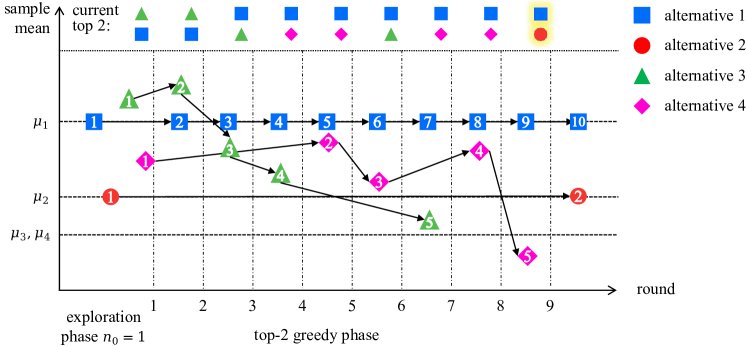
Figure 1: Top-2 greedy sampling process of an example problem with $4$ alternatives where $\bar{X}_{1}(n)=\mu_{1}$ and $\bar{X}_{2}(n)=\mu_{2},\forall n\geq 1$. Numbers in the markers represent the total sample sizes.

Additionally, by the virtue of definition, it is straightforward that $T_{\mathcal{S}^{*}}^{j}=\argmin_{n\geq n_{0}}\bar{X}_{j}(n)$ for any $j\in\mathcal{S}^{*}$. By plugging Equation (7) into (6), we can obtain a lower bound for the desired PCS_m:

$$\mbox{PCS}_{m} \geq \Pr\left\{B-n_{0}k\geq m\left[\sum_{i\in\mathcal{K}\setminus\mathcal{S}^{*}}\left\{N_{i}(X^{**};n_{0})-n_{0}\right\}+\sum_{j\in\mathcal{S}^{*}}\left\{\argmin_{n\geq n_{0}}\bar{X}_{j}(n)-n_{0}\right\}\right]\right\}$$ (8)

$$= \Pr\left\{B-n_{0}k\geq m\left[\sum_{i\in\mathcal{K}\setminus\mathcal{S}^{*}}N_{i}(X^{**};n_{0})+\sum_{j\in\mathcal{S}^{*}}\argmin_{n\geq n_{0}}\bar{X}_{j}(n)-n_{0}k\right]\right\}.$$

Equation (8) showcases the power of a boundary-crossing perspective for analyzing the performance of the EFG-$m$ procedure. Although it seems complicated, it enables us to prove the sample optimality and consistency of the EFG-$m$ procedure.

3.3 From PCS_m to PGS_m

Now we extend the boundary-crossing analysis developed above to study the PGS_m, where the number of good alternatives is greater than $m$, i.e., $|\mathcal{G}|>m$. For the PCS_m scenario detailed in Section 3.2, the boundary, which is a crucial element in the boundary-crossing framework, can be clearly defined by the optimal subset $\mathcal{S}^{*}$. However, such a boundary is no longer readily available when the target turns into selecting a good subset from a pool of good alternatives $\mathcal{G}$. This arises from the existence of multiple viable good subsets within $\mathcal{G}$, each potentially suggesting a different choice of the boundary.

To address the challenge, we define the minimum running average of each good alternative $l$ in $\mathcal{G}$ as $\bar{X}_{l}^{*}=\argmin_{n\geq n_{0}}\bar{X}_{l}(n)$. These values are then ranked in descending order:

$$\bar{X}_{(1)}^{*}\geq\bar{X}_{(2)}^{*}\geq\dots\geq\bar{X}_{(g)}^{*},$$ (9)

where $g=|\mathcal{G}|$. For illustrative purposes, consider a simple scenario where each good alternative is observed without any random noise, such that $\bar{X}_{l}(n)\equiv\mu_{l}$ for all $n\geq n_{0}$ and all $l\in\mathcal{G}$. In this ideal scenario, the top $m$ alternatives (specifically alternatives $1,2,\dots,m$) will consistently outperform all the other alternatives and continue to be sampled until the end of procedure, whenever the running averages of all inferior alternatives in $\mathcal{K}\setminus\mathcal{G}$ fall below $\mu_{m}$, namely the $m$th largest mean. Thus, $\mu_{m}$ effectively acts as the boundary. Extending this logic to the general case with random noise, we analogously set the boundary as $\bar{X}_{(m)}^{*}$, which represents the $m$th largest value among the minimum running averages $\bar{X}_{(1)}^{*},\bar{X}_{(1)}^{*},\dots,\bar{X}_{(g)}^{*}$. It is important to notice that the boundary $\bar{X}_{(m)}^{*}$ is determined by the entire set of good alternatives. This frees us from having to select a specific subset of good alternatives to determine the boundary, but rather automatically sets the boundary according to the sampling processes of all good alternatives.

Given the boundary $\bar{X}_{(m)}^{*}$, the boundary-crossing times of all inferior alternatives can be observed as follows, which is an analogous result to Observation 1 for the PCS_m scenario.

Observation 3

For each inferior alternative $i\in\mathcal{K}\setminus\mathcal{G}$, its sample size can be upper bounded by the boundary-crossing time

$$N_{i}(\bar{X}^{*}_{(m)};n_{0}):=\inf\{n\geq n_{0}:\bar{X}_{i}(n)\leq\bar{X}^{*}_{(m)}\}.$$ (10)

Additionally, the boundary $\bar{X}_{(m)}^{*}$ basically divides the good alternatives in $\mathcal{G}$ into two disjoint subsets: $\mathcal{G}^{\prime}=\{(1),(2),\dots,(m)\}$ and $\mathcal{G}^{\prime\prime}=\{(m+1),(m+2),\dots,(g)\}$. Notice that for each alternative $l$ from $\mathcal{G}^{\prime\prime}$, whenever it achieves the minimum running average $\bar{X}_{l}^{*}$, its sample mean will remain consistently smaller than those of the $m$ alternatives in $\mathcal{G}^{\prime}$, by Equation (9). Then, it is straightforward to obtain the following interesting observation about the good alternatives in $\mathcal{G}^{\prime\prime}$.

Observation 4

All the good alternatives from $\mathcal{G}^{\prime\prime}$ will be ultimately dominated by the $m$ good alternatives in $\mathcal{G}^{\prime}$. Additionally, for each alternative $l\in\mathcal{G}^{\prime\prime}$, its sample size can be upper bounded by $\argmin_{n\geq n_{0}}\bar{X}_{l}(n)$.

As we can see from Observations 3 and 4, the good alternatives included in $\mathcal{G}^{\prime}$ ultimately dominates not only all the inferior alternatives in $\mathcal{K}\setminus\mathcal{G}$ but also the other good alternatives in $\mathcal{G}^{\prime\prime}$, as the sampling process proceeds. Specifically, when this fact occurs within the sampling budget $B$, the EFG-$m$ selects the subset $\mathcal{G}^{\prime}$ at terminal round, leading to a good selection. To formally capture this behavior, we can introduce an observation analogous to Observation 2.

Observation 5

A good selection is ensured if the simulation budget in the sampling phase, i.e., $B-n_{0}k$, is sufficient to cover the following three kinds of key timelines:

1. $T_{\mathcal{G}^{\prime}}^{j}\,(j\in\mathcal{G}^{\prime})$, the number of greedy sampling rounds on alternatives $j\in\mathcal{G}^{\prime}$ such that its minimum running average $\bar{X}_{j}^{*}$ is reached;

2. $T_{\mathcal{K}\setminus\mathcal{G}}$, the number of greedy sampling rounds on the inferior alternatives in $\mathcal{K}\setminus\mathcal{G}$ such that all their running averages first drop below $\bar{X}^{*}_{(m)}$;

3. $T_{\mathcal{G}^{\prime\prime}}^{l}\,(l\in\mathcal{G}^{\prime\prime})$, the number of greedy sampling rounds on good alternative $l\in\mathcal{G}^{\prime\prime}$ such that its minimum running average $\bar{X}_{l}^{*}$ is reached.

Compared to its analogous Observation 2, Observation 5 involves an additional timeline $T_{\mathcal{G}^{\prime\prime}}^{l}$, which is crucial for tracking the sample dynamic of the good alternatives within $\mathcal{G}^{\prime\prime}$. Then, the PGS_m can be expressed as

$$\mbox{PGS}_{m}\geq\Pr\left\{B-n_{0}k\geq m\sum_{j\in\mathcal{G}^{\prime}}T_{\mathcal{G}^{\prime}}^{j}+mT_{\mathcal{K}\setminus\mathcal{G}}+m\sum_{l\in\mathcal{G}^{\prime\prime}}T_{\mathcal{G}^{\prime\prime}}^{l}\right\}.$$ (11)

Similarly to Equation (7), we have

$$T_{\mathcal{K}\setminus\mathcal{G}}\leq\ \sum_{i\in\mathcal{K}\setminus\mathcal{G}}\left\{N_{i}(\bar{X}_{(m)}^{*};n_{0})-n_{0}\right\}.$$ (12)

Meanwhile, Observations 3 and 4 show that

$$T_{\mathcal{G}^{\prime}}^{j}=\argmin_{n\geq n_{0}}\bar{X}_{j}(n)-n_{0},\mbox{ and }T_{\mathcal{G}^{\prime\prime}}^{l}=\argmin_{n\geq n_{0}}\bar{X}_{l}(n)-n_{0}.$$ (13)

Plugging Equations (12) and (13) into (11) leads to

$$\mbox{PGS}_{m} \geq\ \Pr\left\{B-n_{0}k\geq m\left[\sum_{i\in\mathcal{K}\setminus\mathcal{G}}\left\{N_{i}(X_{(m)}^{*};n_{0})-n_{0}\right\}+\sum_{j\in\mathcal{G}}\left\{\argmin_{n\geq n_{0}}\bar{X}_{j}(n)-n_{0}\right\}\right]\right\}$$ (14)

$$\geq\ \Pr\left\{B-n_{0}k\geq m\left[\sum_{i\in\mathcal{K}\setminus\mathcal{G}}N_{i}(X_{(m)}^{*};n_{0})+\sum_{j\in\mathcal{G}}\argmin_{n\geq n_{0}}\bar{X}_{j}(n)-n_{0}k\right]\right\}.$$

The PGS_m lower bound above is an extension of the PCS_m lower bound in Equation (8). When $\mathcal{S}^{*}=\mathcal{G}$, these two lower bounds become identical. In addition, it is worth acknowledging that the PGS_m lower bound may not be tight. It is because it is constructed based on a particular scenario that leads to a good selection. Nonetheless, as we will show in the following section, this PGS_m lower bound is sufficient to establish the sample optimality and consistency of the EFG-$m$ procedure.

4 Properties of the EFG-$\mathbf{m}$ Procedure

In this section, we prove the desired large-scale statistical properties of the EFG-$m$ procedure, particularly its sample optimality and consistency in terms of the PGS_m. We first introduce a necessary assumption on the problem configuration in the asymptotic regime as $k\to\infty$.

There exists a positive constant $\bar{\sigma}$ such that $\max\limits_{i\in\mathcal{K}}\sigma_{i}^{2}\leq\bar{\sigma}^{2}$ regardless of how large the problem scale $k$ is. This assumption helps to prevent scenarios where the variances of some alternatives could become unbounded as $k$ increases. Importantly, it is worth noting that the value of the variance bound $\bar{\sigma}^{2}$ does not need to be known for the implementation and analysis of our EFG-$m$ procedure.

Meanwhile, we also include here the boundedness assumption on the number of good alternatives (i.e., $|\mathcal{G}|$), which has been explained in Section 2.2. It helps to streamline our analysis and understanding of the desired properties of EFG-$m$. For scenarios where this assumption is violated, as we show in Section 6.2, proper modifications can be made to the EFG-$m$ procedure such that it enables to effectively address the scenarios. There exists a positive constant $\bar{g}$ such that $g=|\mathcal{G}|\leq\bar{g}$ regardless of how large $k$ is.

4.1 Sample Optimality

To establish the sample optimality as defined in Definition 2.1, it suffices to verify that the PGS_m lower bound outlined in Equation (14) does not approach to zero as $k\to\infty$, given a linearly growing sampling budget $B=ck$ for some positive constant $c$. For ease of presentation, we rewrite Equation (14) as

$$\mbox{PGS}_{m}\geq\Pr\left\{\frac{B}{mk}-\frac{n_{0}}{m}+n_{0}\geq\frac{1}{k}\sum_{j\in\mathcal{G}}\argmin_{n\geq n_{0}}\bar{X}_{j}(n)+\frac{1}{k}\sum_{i\in\mathcal{K}\setminus\mathcal{G}}N_{i}\left(X^{*}_{(m)};n_{0}\right)\right\}.$$ (15)

The equation above relates to the properties of the running average process $\{\bar{X}_{i}(n):n=n_{0},n_{0}+1,\dots\}$ for each alternative $i\in\mathcal{K}$, particularly focusing on its minimum or boundary-crossing time. As such, we first summarize two useful lemmas from Li et al. (2024) concerning their properties.

Lemma 4.1

For any alternative $j\in\mathcal{G}$, its running average process $\{\bar{X}_{j}(n):n=n_{0},n_{0}+1,\dots\}$ reaches its minimum within a finite number of observations almost surely, i.e., $\argmin_{n\geq n_{0}}\bar{X}_{j}(n)<\infty$ almost surely.

Lemma 4.2

For any alternative $i\in\mathcal{K}\setminus\mathcal{G}$ and a fixed boundary $x>\mu_{i}$, its associated boundary-crossing time $N_{i}\left(x;n_{0}\right)$ of the running average process $\{\bar{X}_{i}(n):n=n_{0},n_{0}+1,\dots\}$ has a finite expectation. Specifically,

$$\mathrm{E}[N_{i}(x;n_{0})]\leq C\left(\frac{x-\mu_{i}}{\bar{\sigma}};n_{0}\right),$$

where $C(z;n_{0})=\mathrm{E}[\inf\{n\geq n_{0}:\bar{Z}(n)\leq z\}]$ and $\{\bar{Z}(n):n=n_{0},n_{0}+1,\dots\}$ denotes the running average process of a sequence of independent standard normal random variables.

Based on the two lemmas, we establish the sample optimality of the EFG-$m$ by first presenting two key arguments. These arguments not only sketch our proof, but also explain the insights behind the sample optimality.

Argument 1

$\sum\limits_{j\in\mathcal{G}}\argmin_{n\geq n_{0}}\bar{X}_{j}(n)<\infty$ almost surely.

Argument 1 is straightforward by combining Assumption 4 and Lemma 4.1. It indicates that all the good alternatives in $\mathcal{G}$ are guaranteed to reach the minimums of their running averages within a finite number of observations almost surely. Consequently, the boundary $\bar{X}_{(m)}^{*}$ specified in the boundary-crossing framework of the EFG-$m$ procedure can also be reached within a finite number of observations almost surely. This implies, given the sampling budget $B=ck$ as $k\to\infty$, the requirement of reaching the boundary $\bar{X}_{(m)}^{*}$ does not affect the sample optimality.

Argument 2

Under the condition $\bar{X}^{*}_{(m)}\geq\mu_{m}-\delta_{0}$ with $\delta_{0}\in(0,\delta)$, $\limsup\limits_{k\to\infty}\,\frac{1}{k}\sum\limits_{i\in\mathcal{K}\setminus\mathcal{G}}N_{i}(\bar{X}^{*}_{(m)};n_{0})\leq C\left(\frac{\delta-\delta_{0}}{\bar{\sigma}};n_{0}\right)$ almost surely.

Under the condition $\bar{X}^{*}_{(m)}\geq\mu_{m}-\delta_{0}$, for each inferior alternative $i\in\mathcal{K}\setminus\mathcal{G}$, because $\mu_{i}<\mu_{m}-\delta$,

$$\begin{aligned} N_{i}\left(X^{*}_{(m)};n_{0}\right)&=\ \inf\left\{n\geq n_{0}:\bar{X}_{i}(n)\leq\bar{X}^{*}_{(m)}\right\}\\ &\leq\ \inf\left\{n\geq n_{0}:\bar{X}_{i}(n)\leq\mu_{m}-\delta_{0}\right\}\\ &\leq\ \inf\left\{n\geq n_{0}:\bar{X}_{i}(n)\leq\mu_{i}+\delta-\delta_{0}\right\}\\ &=\ N_{i}\left(\mu_{i}+\delta-\delta_{0};n_{0}\right).\end{aligned}$$

By the independence of $N_{i}\left(\mu_{i}+\delta-\delta_{0};n_{0}\right),i\in\mathcal{K}\setminus\mathcal{G}$, we may use the strong law of large numbers (SLLN) and Lemma 4.2 to obtain Argument 2.

Argument 2 highlights an important feature of the EFG-$m$ procedure that, whenever the condition $\bar{X}^{*}_{(m)}\geq\mu_{m}-\delta_{0}$ is satisfied, the maximal sampling budget allocated to all the inferior alternatives, quantified by the sum of their corresponding boundary-crossing times, is $\mathcal{O}(k)$. This feature is crucial to understand the sample optimality of the EFG-$m$ procedure. It also suggests that the PGS_m might be closely related to the probability of fulfilling the condition $\bar{X}^{*}_{(m)}\geq\mu_{m}-\delta_{0}$.

Building on the two arguments above, we can rigorously prove the sample optimality of the EFG-$m$ procedure, which is presented in the following theorem. The detailed proof is deferred to 10.1.

Theorem 4.3

Suppose that Assumptions 4 and 4 hold. If the total sampling budget $B=(n_{0}+n_{g})k$ and $n_{g}>m\left[C\left(\frac{\delta}{\bar{\sigma}};n_{0}\right)-n_{0}\right]$, the PGS_m of the EFG-$m$ procedure satisfies

$$\liminf\limits_{k\to\infty}\mbox{PGS}_{m}\geq\Pr\left\{\bar{X}_{(m)}^{*}\geq\mu_{m}-\delta_{0}\right\}>0,$$ (16)

where $\delta_{0}\in(0,\delta)$ is a constant such that $m\left[C\left(\frac{\delta-\delta_{0}}{\bar{\sigma}};n_{0}\right)-n_{0}\right]=n_{g}$. Therefore, the EFG-$m$ procedure is sample optimal.

Notice that the PGS_m lower bound $\Pr\left\{\bar{X}_{(m)}^{*}\geq\mu_{m}-\delta_{0}\right\}$ above is not tight. But it aligns well with our intuitive understandings of the PGS_m. By Equation (9), $\bar{X}_{(m)}^{*}$ is the $m$th order statistics among the minimum running averages of $g$ good alternatives in $\mathcal{G}$. The lower bound $\Pr\left\{\bar{X}_{(m)}^{*}\geq\mu_{m}-\delta_{0}\right\}$ refers to the probability that at least $m$ of the $g$ good alternatives maintain their running averages above a constant $\delta-\delta_{0}$, which generally increases as $g$ increase. This supports our practical observation that including more good alternatives often result in a higher PGS_m.

4.2 Consistency

We further prove the consistency of the EFG-$m$ procedure. By the definition of consistency in Definition 2.2, it suffices to show that, for any $\alpha\in(0,1)$, these exists a pair of $n_{0}$ and $n_{g}$ such that

$$\liminf_{k\to\infty}\,\mbox{PGS}_{m}\geq 1-\alpha.$$

With Theorem 4.3, we may first reformulate the limiting PGS_m above in a more tractable form:

$$\liminf_{k\to\infty}\mbox{PGS} \geq \Pr\left\{\bar{X}_{(m)}^{*}\geq\mu_{m}-\delta_{0}\right\}$$

$$\geq \Pr\left\{\bar{X}_{1}^{*}\geq\mu_{m}-\delta_{0},\bar{X}_{2}^{*}\geq\mu_{m}-\delta_{0},\dots,\bar{X}_{m}^{*}\geq\mu_{m}-\delta_{0}\right\}$$

$$= \prod_{j=1\ldots,m}\Pr\left\{\min_{n\geq n_{0}}\bar{X}_{j}(n)\geq\mu_{m}-\delta_{0}\right\}$$

$$\geq \prod_{j=1\ldots,m}\Pr\left\{\min_{n\geq n_{0}}\bar{X}_{j}(n)\geq\mu_{j}-\delta_{0}\right\}\qquad(\mbox{because }\mu_{j}\geq\mu_{m}).$$

Then our task is modified to find a pair of $n_{0}$ and $n_{g}$ such that

$$\prod_{j=1\ldots,m}\Pr\left\{\min_{n\geq n_{0}}\bar{X}_{j}(n)\geq\mu_{j}-\delta_{0}\right\}\geq 1-\alpha.$$ (17)

To proceed, we need the following lemma and its proof is included in 10.2.

Lemma 4.4

Suppose that Assumption 4 holds. Then, we have:

$$\Pr\left\{\min_{n\geq n_{0}}\bar{X}_{j}(n)>\mu_{j}-\delta_{0}\right\}\geq 1-2\exp\left(-\frac{n_{0}\delta_{0}^{2}}{2\bar{\sigma}^{2}}\right).$$

Using Lemma 4.4, we may readily derive the left-hand-side term in Equation (17) as:

$$\prod_{j=1\ldots,m}\Pr\left\{\min_{n\geq n_{0}}\bar{X}_{j}(n)\geq\mu_{j}-\delta_{0}\right\}\geq\left[1-2\exp\left(-\frac{n_{0}\delta_{0}^{2}}{2\bar{\sigma}^{2}}\right)\right]^{m}\geq 1-2m\exp\left(-\frac{n_{0}\delta_{0}^{2}}{2\bar{\sigma}^{2}}\right),$$

When $\delta_{0}$ is fixed to be $\delta/2$, for $\alpha\in(0,1)$, we may choose $n_{0}$ as $n_{0}=\frac{8\bar{\sigma}^{2}}{\delta^{2}}\log\left(\frac{2m}{\alpha}\right)$, and subsequently determine $n_{g}$ using the formula $n_{g}=m\left[C\left(\frac{\delta-\delta_{0}}{\bar{\sigma}};n_{0}\right)-n_{0}\right]$ as outlined in Theorem 4.3. Such choice of $n_{0}$ and $n_{g}$ ensures that Equation (17) is met, thereby confirming the consistency of the EFG-$m$ procedure is verified. We formally present this result in the following theorem and its proof is included in 10.3.

Theorem 4.5

Suppose that Assumptions 4 and and 4 hold. For any $\alpha\in(0,1)$, if the total sampling budget $B=(n_{0}+n_{g})k$ with $n_{0}=\frac{8\bar{\sigma}^{2}}{\delta^{2}}\log\frac{2m}{\alpha}$ and $n_{g}\geq\frac{\alpha}{2}+\frac{4\alpha\bar{\sigma}^{2}}{\delta^{2}}$, the PGS_m of the EFG-$m$ procedure satisfies $\liminf_{k\to\infty}\mbox{PGS}_{m}\geq 1-\alpha$. Thus, the EFG-$m$ procedure is consistent.

Theorem 4.5 not only confirms the consistency of the EFG-$m$ procedure, but also points out another important property of the procedure. Notice that Theorem 4.5 provides a feasible way to turn the fixed-budget EFG-$m$ into a fixed-precision procedure when $\bar{\sigma}$ and $\delta$ are known. In the best-armed-identification (BAI) literature, which is closely related to our OSS problem, the worse-case sample complexity is an important measure. It determines the minimum number of samples required to select a good subset of size $m$ with given fixed precision. The recognized lower bound for worst-case sample complexity in the BAI literature at least $\mathcal{O}\left(\frac{k}{\delta^{2}}\log\left(\frac{m}{\alpha}\right)\right)$(Kalyanakrishnan et al. 2012), indicating that any procedure must meet this lower bound. It is straightforward from Theorem 4.5 that the sample complexity of the EFG-$m$, namely $k(n_{0}+n_{g})$, aligns with the established sample complexity bound. This shows that the EFG-$m$ procedure is optimal regarding the sample complexity in the asymptotic regime as $k\to\infty$.

5 Ranking within the Selected Subset

As previously mentioned in Section 1, for better supporting decision-making, it is valuable to not only select a subset of top-performing alternatives but also correctly rank the alternatives within the subset. To address this, we first introduce a new concept of indifference-based ranking for large-scale OSS problems where the means of alternatives may be very close to each other. We then investigate the effectiveness of the EFG-$m$ procedure in delivering both good selection and ranking.

5.1 Indifference-based Ranking

When the total sampling budget $B$ is exhausted, the EFG-$m$ procedure selects the subset $\mathcal{S}$ based on the terminal sample means of alternatives in $\mathcal{K}$. Let $\{\pi_{1}(\mathcal{S}),\pi_{2}(\mathcal{S}),\dots,\pi_{m}(\mathcal{S})\}\subset\mathcal{K}$ denote the indices of alternatives included in $\mathcal{S}$. For simplicity, we let $\pi_{1}(\mathcal{S})<\pi_{2}(\mathcal{S})<\dots<\pi_{m}(\mathcal{S})$, indicating $\mu_{\pi_{1}(\mathcal{S})}\geq\mu_{\pi_{2}(\mathcal{S})}\geq\dots\geq\mu_{\pi_{m}(\mathcal{S})}$. To obtain a ranking of these alternatives, the most straightforward method is by sorting their sample means in descending order. The alternative with a larger sample mean is assigned a higher rank. Clearly, the resulting ranking is correct if

$$\bar{X}_{\pi_{1}(\mathcal{S})}(n_{\pi_{1}(\mathcal{S})}(B))>\bar{X}_{\pi_{2}(\mathcal{S})}(n_{\pi_{2}(\mathcal{S})}(B))>\dots>\bar{X}_{\pi_{m}(\mathcal{S})}(n_{\pi_{m}(\mathcal{S})}(B)),$$

where $n_{\pi_{i}(\mathcal{S})}(B)$ denotes the sample size allocated to alternative $\pi_{i}(\mathcal{S})\in\mathcal{S}$ at the end of procedure.

Recall that we introduced an indifference-zone parameter $\delta>0$ in Section 2. It refers to the minimal mean difference among alternatives that decision makers feel worthy detecting. Any two alternatives whose mean difference is within $\delta$ are considered indifferent for selection purpose. It follows logically that the ranking between these two alternatives should also be treated as indifferent. To formally extend this concept of indifference to the ranking purpose, we adopt the semiordering principle from Luce (1956) and define the indifference-based ranking (IBR) among alternatives. The IBR consists of two binary relations depending on the indifference-zone parameter $\delta$: indifference ($\sim_{\delta}$) and dominance ($>_{\delta}$). These two relations are formalized as follows.

Definition 5.1

Given an indifference-zone parameter $\delta>0$, for any two alternatives $A$ and $B$ whose means are denoted by $\mu_{A}$ and $\mu_{B}$, define

• $A\sim_{\delta}B$ if and only if $|\mu_{A}-\mu_{B}|<\delta$;

• $A>_{\delta}B$ if and only if $\mu_{A}-\mu_{B}\geq\delta$.

Notice that the dominance relation “$>_{\delta}$” above is transitive. More specifically, for any three alternatives $A$, $B$ and $C$, if $A>_{\delta}B$ (i.e., $\mu_{A}-\mu_{B}\geq\delta$) and $B>_{\delta}C$ (i.e., $\mu_{B}-\mu_{C}\geq\delta$), then it must be true that $A>_{\delta}C$, because $\mu_{A}-\mu_{C}=\mu_{A}-\mu_{B}+\mu_{B}-\mu_{C}\geq 2\delta>\delta$. This transitive property is crucial to ensure consistency when alternatives are ranked based on their pairwise dominance.

With IBR, we are ready to define a good ranking (GR) within the selected subset $\mathcal{S}$. Compared to the case of correct ranking, we only need to care about the correctness of ranking among alternatives which exhibits dominance relations. By the transitivity property of dominance relation in Definition 5.1, we declare that a good ranking (GR) of $\mathcal{S}$ is obtained if the following condition

$$\bar{X}_{\pi_{i}(S)}(n_{\pi_{i}(S)}(B))>\bar{X}_{\pi_{j}(S)}(n_{\pi_{j}(S)}(B)),\mbox{ if }\pi_{i}(\mathcal{S})>_{\delta}\pi_{j}(\mathcal{S}),\ \forall\pi_{i}(\mathcal{S})\pi_{j}(\mathcal{S})\in\mathcal{S}$$

is satisfied, or equivalently in a neater form

$$\bar{X}_{i}(n_{i}(B))>\bar{X}_{j}(n_{j}(B)),\mbox{ if }\mu_{i}-\mu_{j}\geq\delta,\ \forall i,j\in\mathcal{S}.$$ (18)

To measure the effectiveness of the EFG-$m$ procedure when considering both the selection and ranking, we propose a new metric called the probability of good selection and ranking (PGSR_m), which is expressed as

$$\mbox{PGSR}_{m}=\Pr\left\{\{\mathcal{S}\subset\mathcal{G}\}\cap\left\{\bar{X}_{i}(n_{i}(B))>\bar{X}_{j}(n_{j}(B))\mbox{ if }\mu_{i}-\mu_{j}>\delta,\forall i,j\in\mathcal{S}\right\}\right\}.$$ (19)

The definition of PGSR_m allows us to measure the performance of a procedure for good selection and ranking when solving large-scale OSS problems.

5.2 PGSR_m of the EFG-$\mathbf{m}$ Procedure

Similar to the PGS_m analysis, we may leverage the boundary-crossing framework to form a lower bound for the PGSR_m. As noticed in Observation 5 or Equation (11), after at most

$$T_{GS}=\sum_{j\in\mathcal{G}^{\prime}}T_{\mathcal{G}^{\prime}}^{j}+\sum_{l\in\mathcal{G}^{\prime\prime}}T_{\mathcal{G}^{\prime\prime}}^{l}+T_{\mathcal{K}\setminus\mathcal{G}}$$ (20)

rounds of greedy sampling, the EFG-$m$ procedure will concentrate the sampling on the set of good alternatives in $\mathcal{G}^{\prime}$ until the end of procedure. Consequently, a GS event is ensured and the subset

$$\mathcal{S}=\mathcal{G}^{\prime}=\{(1),(2),\dots,(m)\}$$

is selected. When taking PGSR_m into consideration, we are required to additionally ensure the GR within $\mathcal{G}^{\prime}$, or equivalently, the condition detailed in Equation (18). Then, beyond the PGS_m analysis, the key challenge in analyzing the PGSR_m is to investigate how many additional rounds, if necessary, are required to satisfy condition (18).

Suppose that the terminal sample mean of each alternative $j\in\mathcal{G}^{\prime}$ lies within $\delta/2$ of its true mean, namely,

$$|\bar{X}_{j}(n_{j}(B))-\mu_{j}|<\delta/2.$$ (21)

Then, condition (18) can be straightforwardly met because, for any alternatives $i,j\in\mathcal{G}^{\prime}$ with $\mu_{i}-\mu_{j}\geq\delta$,

$$\bar{X}_{i}(n_{i}(B))-\bar{X}_{j}(n_{j}(B))=\left[\bar{X}_{i}(n_{i}(B))-\mu_{i}\right]-\left[\bar{X}_{i}(n_{i}(B))-\mu_{i}\right]+\left[\mu_{i}-\mu_{j}\right]>-\delta/2-\delta/2+\delta=0.$$

To formally present the insight above, we define

$$L^{j}_{\mathcal{G}^{\prime}}\left(\delta/2;n_{0}\right)=\sup\left\{n\geq n_{0}:|\bar{X}_{j}(n)-\mu_{j}|\geq\delta/2\right\}$$ (22)

as the last exit time of the running average process $\{\bar{X}_{j}(n):n=n_{0},n_{0}+1,\dots\}$ of alternative $j$ from the region $[\mu_{j}-\delta/2,\mu_{j}+\delta/2]$ after $n=n_{0}$. By definition, once the sample size allocated to alternative $j$ exceeds $L^{j}_{\mathcal{G}^{\prime}}(\delta/2;n_{0})$, its sample mean will remain satisfying Equation (21) until the end of procedure. In light of this, we tailor Observation 5 for GS into the following Observation 6 for the context of ensuring both good selection and ranking. Compared to Observation 5, Observation 6 includes a new timeline $L^{j}_{\mathcal{G}^{\prime}}(\delta/2;n_{0})-n_{0}$, which is marked as the second point, such that condition (18) can be satisfied.

Observation 6

A good selection and selection is ensured if the sampling budget in the greedy phase, i.e., $B-n_{0}k$, is sufficient to cover the following four kinds of key timelines:

1. $T_{\mathcal{G}^{\prime}}^{j}\,(j\in\mathcal{G}^{\prime})$, the number of greedy sampling rounds on alternatives $j\in\mathcal{G}^{\prime}$ such that its minimum running average $\bar{X}_{j}^{*}$ is reached;

2. $L^{j}_{\mathcal{G}^{\prime}}(\delta/2;n_{0})-n_{0}$, the number of greedy sampling rounds on alternatives $j\in\mathcal{G}^{\prime}$ such that its running average $\bar{X}_{j}^{*}$ remains within $\delta/2$ of its true mean $\mu_{j}$;

3. $T_{\mathcal{K}\setminus\mathcal{G}}$, the number of greedy sampling rounds on the inferior alternatives in $\mathcal{K}\setminus\mathcal{G}$ such that all their running averages first drop below $\bar{X}^{*}_{(m)}$;

4. $T_{\mathcal{G}^{\prime\prime}}^{l}\,(l\in\mathcal{G}^{\prime\prime})$, the number of greedy sampling rounds on good alternative $l\in\mathcal{G}^{\prime\prime}$ such that its minimum running average $\bar{X}_{l}^{*}$ is reached.

From the observation above, the maximum number of greedy sampling rounds, $T_{GSR}$, to deliver a good selection and ranking is

$$\begin{aligned} T_{GSR}&=\ \sum_{j\in\mathcal{G}^{\prime}}\max\left\{T_{\mathcal{G}^{\prime}}^{j},L_{\mathcal{G}^{\prime}}^{j}(\delta/2;n_{0})-n_{0}\right\}+T_{\mathcal{K}\setminus\mathcal{G}}+\sum_{l\in\mathcal{G}^{\prime\prime}}T_{\mathcal{G}^{\prime\prime}}^{l}\\ &=\ \sum_{j\in\mathcal{G}^{\prime}}\left(L_{\mathcal{G}^{\prime}}^{j}(\delta/2;n_{0})-T_{\mathcal{G}^{\prime}}^{j}\right)^{+}+\sum_{j\in\mathcal{G}^{\prime}}T_{\mathcal{G}^{\prime}}^{j}+T_{\mathcal{K}\setminus\mathcal{G}}+\sum_{l\in\mathcal{G}^{\prime\prime}}T_{\mathcal{G}^{\prime\prime}}^{l},\end{aligned}$$ (23)

where $x^{+}=\max\{x,0\}$. Notice that, in contrast to its analogous term $T_{GS}$ in Equation (20), $T_{GSR}$ involves a new component $\sum_{j\in\mathcal{G}^{\prime}}\left(L_{\mathcal{G}^{\prime}}^{j}(\delta/2;n_{0})-\argmin_{n\geq n_{0}}\bar{X}_{j}(n)\right)^{+}$. This component essentially represents the extra sampling rounds required to ensure good ranking within the selected subset $\mathcal{G}^{\prime}$.

Furthermore, Observation 6 shows that, within a limited sampling budget $B$, a good selection and ranking is guaranteed if $B\geq n_{0}k+mT_{GSR}$. In other words, the PGSR_m can be expressed as

$$\mbox{PGSR}_{m} \geq \Pr\left\{B-n_{0}k\geq m\left[\sum\limits_{j\in\mathcal{G}^{\prime}}\left(L_{\mathcal{G}^{\prime}}^{j}(\delta/2;n_{0})-T_{\mathcal{G}^{\prime}}^{j}\right)^{+}+\sum\limits_{j\in\mathcal{G}^{\prime}}T_{\mathcal{G}^{\prime}}^{j}+T_{\mathcal{K}\setminus\mathcal{G}}+\sum\limits_{l\in\mathcal{G}^{\prime\prime}}T_{\mathcal{G}^{\prime\prime}}^{l}\right]\right\}$$ (24)

$$\geq \Pr\left\{B-n_{0}k\geq m\left[\sum\limits_{j\in\mathcal{G}^{\prime}}\left(L_{\mathcal{G}^{\prime}}^{j}(\delta/2;n_{0})-\underset{n\geq n_{0}}{\argmin}\bar{X}_{j}(n)\right)^{+}\right.\right.$$

$$\qquad\qquad\qquad\qquad\left.\left.+\sum\limits_{l\in\mathcal{G}}\underset{n\geq n_{0}}{\argmin}\bar{X}_{l}(n)+\sum\limits_{i\in\mathcal{K}\setminus\mathcal{G}}N_{i}(\bar{X}^{*}_{(m)};n_{0})-n_{0}k\right]\right\},$$

where the last inequality holds from Equations (12) and (13). It is worth noticing that the PGSR_m lower bound is no larger than the the PGS_m lower bound presented in Equation (14). This supports our intuition that ensuring both good selection and ranking is often more challenging than achieving merely good selection.

5.3 Sample Optimality and Consistency for the PGSR_m

By repeating the arguments in Section 4, we may easily prove the sample optimality and consistency of the EFG-$m$ procedure in terms of PGSR_m. The key distinction in this analysis involves evaluating the newly added component $\sum_{j\in\mathcal{G}^{\prime}}\left(L_{\mathcal{G}^{\prime}}^{j}(\delta/2;n_{0})-\argmin_{n\geq n_{0}}\bar{X}_{j}(n)\right)^{+}$. Interestingly, as we demonstrate in the following lemma, this component becomes negligible as $k\to\infty$, suggesting that it may not significantly influence the asymptotic behavior of PGSR_m. The detailed proof of Lemma 5.2 is included in 10.4.

Lemma 5.2

Suppose that Assumptions 4 and 4 hold. Then we have

$$\limsup_{k\rightarrow\infty}\frac{1}{k}\sum\limits_{j\in\mathcal{G}^{\prime}}\left(L_{\mathcal{G}^{\prime}}^{j}(\delta/2;n_{0})-\argmin_{n\geq n_{0}}\bar{X}_{j}(n)\right)^{+}=0.$$

With this lemma, we can obtain the sample optimality and consistency of the EFG-$m$ procedure in terms of PGSR_m, which are summarized in the following theorem. The detailed proof of the theorem is included in 10.5.

Theorem 5.3

Suppose that Assumptions 4 and 4 hold. If the total sampling budget $B=(n_{0}+n_{g})k$ and $n_{g}>m\left[C\left(\frac{\delta}{\bar{\sigma}};n_{0}\right)-n_{0}\right]$, the PGSR_m of the EFG-$m$ procedure satisfies

$$\liminf\limits_{k\to\infty}\mbox{PGSR}_{m}\geq\Pr\left\{\bar{X}_{(m)}^{*}\geq\mu_{m}-\delta_{0}\right\}>0,$$

where $\delta_{0}\in(0,\delta)$ is a constant such that $m\left[C\left(\frac{\delta-\delta_{0}}{\bar{\sigma}};n_{0}\right)-n_{0}\right]=n_{g}$. Therefore, the EFG-$m$ procedure is sample optimal in terms of PGSR_m. Furthermore, we can show that the EFG-$m$ procedure is also consistent in terms of PGSR_m.

It is worth noticing from the comparison between Theorems 4.3 and 5.3 that the PGS_m and PGSR_m display the same limiting behavior as $k\to\infty$. This equivalence arises because the sampling cost of obtaining the IBR within the selected good subset $\mathcal{G}^{\prime}$ is negligible as $k$ increases. Correspondingly, in our numerical experiments, the PGSR_m of the EFG-$m$ procedure may tend to become identical to the PGS_m when $k$ is sufficiently large, demonstrating the free ranking effect of the EFG-$m$ procedure. To the best of our knowledge, no other OSS procedure in the literature exhibits this particular feature.

6 Procedure Enhancements

In this section, we focus on enhancing the practical efficiency of the EFG-$m$ procedure in addressing large-scale OSS problems. Specifically, in Section 6.1, we improve the procedure by refining its top-$m$ greedy sampling rule. Subsequently, in Section 6.2, we adapt the procedure to accommodate scenarios where the number of good alternatives, $|\mathcal{G}|$, grows to infinity as $k\to\infty$, namely, where Assumption 4 is not met.

6.1 Top-$\mathbf{M}$ Greedy Selection and Adaptive Exploration

The top-$m$ greedy sampling rule in the EFG-$m$ procedure may bring inefficiency, consuming unnecessary sampling budget in the greedy phase. To illustrate this inefficiency, we again consider the simple case where $\mathcal{G}=S^{*}$ and all the top $m$ alternatives are observed without any random noise, such that $\bar{X}_{i}(n)\equiv\mu_{i}$ for all $n\geq n_{0}$ and all $i\in\mathcal{S}^{*}$. From the boundary-crossing perspective introduced in Section 3, a correct selection is assured whenever the sample means of all inferior alternatives falls below the boundary $\mu_{m}$. Ideally, to achieve the highest efficiency, the greedy phase should focus all the sampling budget on the inferior alternatives, so that this condition is met within limited sampling budget. However, the top-$m$ greedy sampling rule does not permit such targeted sampling. Suppose that, at a certain round, the sample means of $q<m$ inferior alternatives are above $\mu_{m}$. The top-$m$ greedy sampling rule will sample on these $q$ alternatives along with $m-q$ alternatives from the top $m$ alternatives, as they have the largest $m$ sample means. Clearly, these $m-q$ observations on the top $m$ alternatives does not aid in achieving a correct selection and thus leads to inefficiency. Moreover, this inefficiency accumulates as the sampling rounds proceed. Although this does not impact the sample optimality or consistency, it may compromise the practical efficiency of the EFG-$m$ procedure.

To mitigate this inefficiency, we modify the greedy sampling phase in the EFG-$m$ procedure by extending the sampling scope from the top $m$ to the top $M$ alternatives at each round, where $M>m$. This strategic adjustment increases the chance of sampling on the inferior alternatives whose sample means exceed the boundary at each round, thus accelerating the accomplishment of boundary crossings of these inferior alternatives. As a direct result, the necessary number of rounds required before achieving a correct selection is reduced, effectively alleviating the cumulative inefficiency over the greedy sampling process. To better illustrate the impact of this adjustment, we also provide a visual comparison of sampling paths under the original top $m$ and the revised top $M$ greedy sampling rules in the following Figure 2. From this figure, we can see that for selecting the top-2 alternatives in the example problem, using a top-3 sampling rule reduces 4 rounds of greedy sampling and thus saves 4 observations compared to using a top-2 sampling rule. The new procedure is referred to as the EFG-$M$ procedure and we detail it in the following Procedure 2. As we will see numerical experiments in Section 7.3 show that when $k$ is relatively large, the EFG-$M$ could improve the performance of the EFG-$m$ procedure by a large margin.

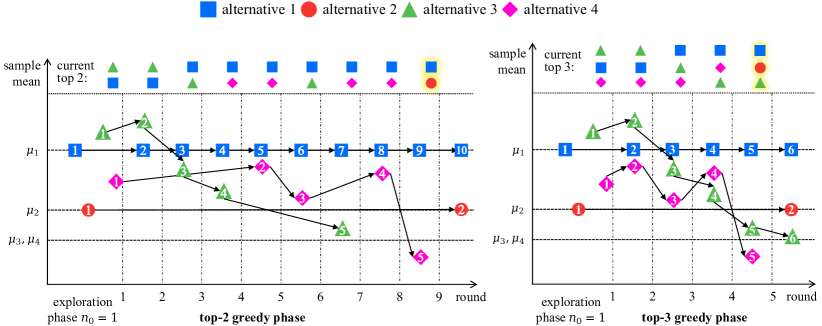
Figure 2: A comparison between top-2 and top-3 greedy sampling processes of an example problem with $4$ alternatives where $\bar{X}_{1}(n)=\mu_{1}$ and $\bar{X}_{2}(n)=\mu_{2},\forall n\geq 1$. Numbers in the markers represent the total sample sizes.

Input: $k$ alternatives $X_{1},\ldots,X_{k}$, the total sampling budget $B=(n_{0}+n_{g})k$, $n_{0}$, $m$ and $M$

1 for $i=1$ to $k$  do // Exploration Phase

2       take $n_{0}$ observations $x_{i1},\ldots,x_{in_{0}}$ from alternative $X_{i}$;

3       set $\bar{X}_{i}(n_{0})=\frac{1}{n_{0}}\sum_{j=1}^{n_{0}}x_{ij}$ and let $n_{i}=n_{0}$;

4      

5 end for

6while $\sum_{i=1}^{k}n_{i}<B$  do // Top-$M$ Greedy Phase

7       let $\mathcal{S}=\,\stackrel{{\scriptstyle 1,\dots,M}}{{\argmax}}_{i\in\{1,\ldots,k\}}\bar{X}_{i}(n_{i})$;

8       for $j\in\mathcal{S}$ do

9             take one observation $x_{j}$ from alternative $X_{j}$;

10             update $\bar{X}_{j}(n_{j}+1)=\frac{1}{n_{j}+1}\left[n_{j}\bar{X}_{j}(n_{j})+x_{j}\right]$ and let $n_{j}=n_{j}+1$;

11            

12       end for

13      

14 end while

Output: $\stackrel{{\scriptstyle 1,\dots,m}}{{\argmax}}_{i\in\{1,\ldots,k\}}\bar{X}_{i}(n_{i})$

Procedure 2 Explore-First Top-$M$ Greedy (EFG-$M$) Procedure

Regarding the EFG-$M$ procedure, we would like to make two remarks. First, the procedure is inherently parallelizable. The exploration phase involves static allocation, which can be easily parallelized. Although the top-$M$ greedy phase is sequential, each round’s task of sampling $M$ different alternatives could be concurrently dispatched to and finished on multiple computing threads (e.g., CPU). Second, the choice of $M(>m)$ may significantly impact on the procedure’s performance. Based on extensive numerical experiments (see, e.g., Section 7.3), we recommend letting $M=2m$ or $M=3m$ to obtain a near-optimal performance.

We further improve the performance of EFG-$M$ procedure by refining the static and equal allocation rule used in the exploration phase. As stated by Hong et al. (2022) and Li et al. (2024), such equal allocation of sampling budget among alternatives might not be optimal. Instead, it would be beneficial if the sampling budget can be concentrated towards the top performing alternatives. To achieve this, they implement an additional seeding phase before the exploration phase, where the seeding information may help allocate more exploration budget to alternatives having better performance. In this paper we adopt this strategy to derive the EFG-$M^{+}$ procedure, a more efficient version of the EFG-$M$ procedure. We include a detailed description of this procedure in 11.1 and demonstrate its superior performance in solving a practical large-scale problem in Section 7.4.

6.2 Alternative Subsampling for Unbounded Number of Good Alternatives

Previous theoretical results are all established based on Assumption 4, which requires the number of good alternatives ($g(k):=|\mathcal{G}|$) to remain bounded as $k$ increases. However, $g(k)$ may grow to infinity as $k\rightarrow\infty$. To deal with this scenario, we consider an alternative subsampling strategy: randomly sampling (with replacement) $mk/g(k)$ alternatives from the entire set of $k$ alternatives first, each chosen with probability $g(k)/k$. This generates a new set of alternatives, termed by $\widetilde{\mathcal{K}}$. As we can show in the following, the appealing feature of $\widetilde{\mathcal{K}}$ is that it maintains a bounded number of good alternatives with a strictly positive probability, independent of the growth in $k$. By implementing the EFG-$m$ procedure on the new set $\widetilde{\mathcal{K}}$, we may revert to the previously considered scenario of bounded number of good alternatives. Further, according to the previous analysis, we may find that the corresponding minimal growth order of $B$ of the EFG-$m$ procedure could be reduced to be $\mathcal{O}(|\widetilde{\mathcal{K}}|)=\mathcal{O}(mk/g(k))$. This suggests that, with the subsampling strategy, this seemingly more complicated scenario may become easier to address.

Let $\widetilde{\mathcal{G}}$ denote the set of good alternatives in $\widetilde{\mathcal{K}}$ and now we investigate the probable boundedness of $|\widetilde{\mathcal{G}}|$. Notice that

$$|\widetilde{\mathcal{G}}|\stackrel{{\scriptstyle d}}{{\sim}}\text{Binomial}\left(\frac{mk}{g(k)},\frac{g(k)}{k}\right)$$

where $\text{Binomial}(n,p)$ represents a binomial random variable with parameters $n$ and $p$. Clearly, the size of $\widetilde{\mathcal{G}}$ is $m$ in expectation, i.e., $\mathrm{E}[|\widetilde{\mathcal{G}}|]=m$. Moreover, we have

$$\Pr\left\{|\widetilde{\mathcal{G}}|\leq m-1\right\}=\Pr\left\{\text{Binomial}\left(\frac{mk}{g(k)},\frac{g(k)}{k}\right)\leq m-1\right\}\leq\frac{1}{2},$$

by Theorem 3.2 of Jogdeo and Samuels (1968), and

$$\Pr\left\{|\widetilde{\mathcal{G}}|\geq 2m+1\right\}=\Pr\left\{\text{Binomial}\left(\frac{mk}{g(k)},\frac{g(k)}{k}\right)\ \geq 2m+1\right\}\leq\frac{m}{2m+1},$$

by the Markov’s inequality. Combining the two inequalities above results in

$$\Pr\left\{m\leq|\widetilde{\mathcal{G}}|\leq 2m\right\}\geq 1-\frac{1}{2}-\frac{m}{2m+1}=\frac{1}{2(2m+1)}$$ (25)

which is strictly positive and does not depend on $k$. It is worth remarking that selecting a subset of $m$ good alternatives from $\widetilde{\mathcal{G}}$ is viable, because Equation (25) ensures that there are consistently at least $m$ good alternatives in $\widetilde{\mathcal{G}}$ with a positive probability as $k$ increases.

7 Numerical Experiments

This section conducts numerical experiments to validate our theoretical results and test the performance of our procedures. Specifically, in Section 7.1, we explore various problem configurations to confirm the sample optimality and consistency of the EFG-$m$ procedure. Then, in Section 7.2, we demonstrate the free ranking effect of the EFG-$m$ procedure. Subsequently, in Section 7.3, we verify the effectiveness of the top-$M$ greedy selection approach as presented in Section 6. Lastly, in Section 7.4, we compare the performance of our procedures and existing OSS procedures in solving a practical large-scale redundancy allocation problem.

7.1 Sample Optimality and Consistency

7.1.1 Sample Optimality.

We start by testing the sample optimality of the EFG-$m$ procedure for the PCS_m and consider two types of problem configurations that are common in the literature: the slippage configuration (SC) and the configuration with decreasing means (DM). To formulate the problem configuration, we first set the distribution of alternative 1 (e.g., $X_{1}\sim\text{Normal}(\mu,\sigma^{2})$), and then use mean shifting to set the distributions of the other alternatives. The mean shifting methods for each SC configuration and DM configuration are described by Equations (26) and (27), respectively,

$$X_{i}\stackrel{{\scriptstyle d}}{{=}}\begin{cases}X_{1}&i=2,\ldots,m,\\ X_{1}-\gamma&i=m+1,\ldots,k;\end{cases}$$ (26)

$$X_{i}\stackrel{{\scriptstyle d}}{{=}}\begin{cases}X_{1}-\frac{i\gamma}{2m}&i=2,\ldots,m,\\ X_{1}-\gamma-\frac{i-(m+1)}{2k}&i=m+1,\ldots,k.\end{cases}$$ (27)

Here, the symbol $\stackrel{{\scriptstyle d}}{{=}}$ denotes the identically distributed relationship between two random variables. In the experiments of this subsection, we set $\gamma=0.1$ and $m=10$.

Notice that despite the convention of assuming normality in designing and analyzing a procedure, it is also of particular interest to test the procedure’s performance for non-normal observations (Nelson et al. 2001, Zhang et al. 2023) to improve its practical applicability. Motivated by this, for both SC and DM configurations, we consider three types of distributions to generate the observations in our experiments: normal, log-normal, and Pareto. As a result, we obtain six problem configurations including SC-Normal, SC-LogNormal, SC-Pareto, DM-Normal, DM-LogNormal and DM-Pareto. Note that the normal, log-normal, and Pareto distributions are all determined by two parameters. We choose the parameter values such that the alternatives of different configurations have similar variances. Details of each problem configuration and the parameter values are summarized in Table 1.

Problem Configuration	Distributional Assumption	Parameters
SC-Normal	$X_{1}\sim\text{Normal}(\mu,\sigma^{2})$	$\mu=0.1$, $\sigma=0.6$
SC-LogNormal	$X_{1}\sim\text{LogNormal}(\mu,\sigma)$	$\mu=-3.7$, $\sigma=1.8$
SC-Pareto	$X_{1}\sim\text{Pareto}(x,a)$	$x=3.1$, $a=0.8$
DM-Normal	$X_{1}\sim\text{Normal}(\mu,\sigma^{2})$	$\mu=0.1$, $\sigma=0.6$
DM-LogNormal	$X_{1}\sim\text{LogNormal}(\mu,\sigma)$	$\mu=-3.7$, $\sigma=1.8$
DM-Pareto	$X_{1}\sim\text{Pareto}(x,a)$	$x=3.1$, $a=0.8$

Table 1: Configurations and Parameters for Optimal Subset Selection Problems

When testing the performance of the EFG-$m$ procedure, we consider multiple values of the number of alternatives $k$, denoted by $k=2^{l}$, with $l$ increasing from 5 to 14, to assess the procedure’s performance across different problem sizes. Under the SC configurations, for each $k$, we set the sample budget $B=500k$, i.e., $c=B/k=500$; under the DM configurations, for each $k$, we set the sample budget $B=400k$, i.e., $c=400$. Given the sample budget $B$, we allocate 80% of the sample budget to the exploration phase, thus letting $n_{0}=0.8c$ and $n_{g}=0.2c$. We also test the existing OCBAm procedure (Chen et al. 2008) and the SAR procedure (Bubeck et al. 2013), comparing them with the EFG-$m$ procedure. Implementation details of these procedures are included in 12.1, where we also discuss some other procedures not being tested. When solving a specific problem, we estimate the PCS_m of each procedure based on 2000 independent macro replications. Then, for each problem configuration, we plot the PCS_m of the three procedures against different $k$ in Figure 3.

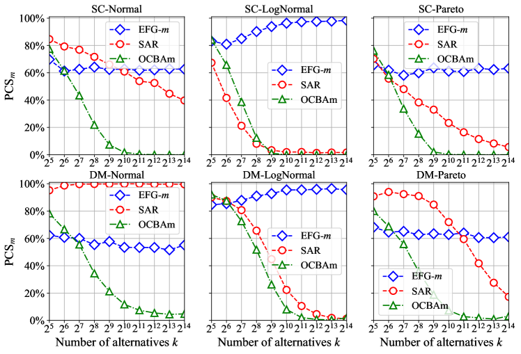
Figure 3: A comparison between the PCS_m of the EFG-$m$, OCBAm and SAR procedures

From Figure 3, we may obtain the following findings. First, our EFG-$m$ procedure is sample optimal for all problem configurations. Taking the SC-Normal configuration as an example, when the number of alternatives $k$ exceeds $2^{6}=64$, the PCS_m of the EFG-$m$ procedure stabilizes around 60%, confirming its sample optimality. Second, the OCBAm procedure is not sample optimal in any case we consider. While the PCS_m of OCBAm might be higher than that of the EFG-$m$ procedure when $k$ is relatively small, as $k$ increases, the EFG-$m$ procedure overtakes the OCBAm procedure. Third, the SAR procedure may be sample optimal for normally distributed observations. Interestingly, under the DM-Normal configuration, the SAR procedure shows a particular advantage; its PCS_m is significantly higher than those of the EFG-$m$ and OCBAm procedures. However, under log-normal or Pareto configurations, the SAR procedure may be no longer sample optimal. Under the SC-LogNormal, SC-Pareto, DM-LogNormal, and DM-Pareto configurations, as $k$ increases, its PCS_m tends to gradually decline to 0. Thus, when $k$ is large, the PCS_m of the EFG-$m$ procedure may be significantly higher than that of the SAR procedure. These results illustrate the robustness of the EFG-$m$ procedure in solving large-scale OSS problems with non-normal observations.

7.1.2 Consistency.

We now proceed to verify the consistency of the EFG-$m$ procedure. For conciseness, we focus on the three SC configurations listed in Table 1. For each SC configuration, we fix the number of alternatives $k=2^{14}$; to demonstrate the trend of PCS_m of the EFG-$m$ procedure as $B=ck$ changes, we set $c$ to increase from 100 to 1000. Then, we plot the PCS_m of the EFG-$m$ procedure again different $c$ for each configuration in Figure 4.

Figure 4: Consistency of the EFG-$m$ procedure for the PCS_m ($B=ck$)

Figure 4 demonstrates the consistency of the EFG-$m$ procedure. Under the three problem configurations, as $c$ in the sample budget $B=ck$ increases, the PCS_m of the EFG-$m$ procedure monotonically rises and ultimately converges to 1. From Figure 4, we can also observe a diminishing marginal effect in the PCS_m growth curve as the sampling budget increases. Once the PCS_m surpasses 60%, the increments in PCS_m become progressively smaller.

Next, we use the SC-Normal configuration to show the optimal sample complexity of the EFG-$m$ procedure regarding various problem parameters. Theorem 4.5 suggests that to maintain the PCS_m of the EFG-$m$ procedure at least $1-\alpha$, where $\alpha\in(0,1)$ is the probability of incorrect selection (PICS_m), the order of $c$ in the total sampling budget $B=ck$ should be $O\left(\frac{\sigma^{2}}{\gamma^{2}}\log\frac{m}{\alpha}\right)$. Initially, we focus on the order of the total sampling budget concerning $\alpha$. Letting the number of alternatives $k=2^{10}$, we fix the other problem parameters and then gradually reduce $\alpha$ from $0.2=\frac{2^{1}}{10}$ to $\frac{2^{-5}}{10}$. For each value of $\alpha$, following Theorem 4.5, we set $n_{0}=\frac{c_{1}\sigma^{2}}{\gamma^{2}}\log\frac{2m}{\alpha}$ and $n_{g}=\frac{\alpha}{2}+\frac{4\alpha\sigma^{2}}{\gamma^{2}}$ where $c_{1}=5.4$ is a constant independent of $\alpha$. For each $\alpha$, we use 30,000 independent macro replications to estimate the EFG-$m$ procedure’s PICS_m. Then, we plot the PICS_m against different $\alpha$ in Figure 5.

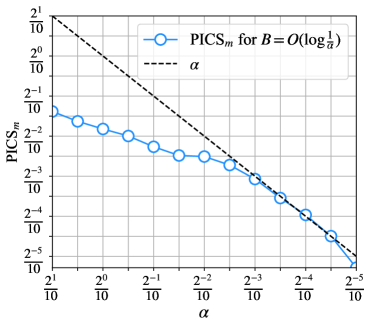
Figure 5: Optimal sample complexity of the EFG-$m$ procedure regarding $\mathbf{\alpha}$

From Figure 5, it can be seen that as $\alpha$ gradually decreases, the PICS_m of the EFG-$m$ procedure also diminishes; when $\alpha$ is sufficiently small, the slope of the EFG-$m$ procedure’s PICS_m is close to -1, demonstrating that it decreases at the same rate as $\alpha$. This phenomenon indicates that setting $c$ as $O\left(\log\frac{1}{\alpha}\right)$ is sufficient to ensure the EFG-$m$ procedure’s PICS_m remains at most $\alpha$. We have also investigated the order of the total sampling budget concerning $\gamma$, $\sigma^{2}$, and $m$. The numerical results further validate Theorem 4.5 and are included in 12.3.

7.2 Free Ranking Effect

This subsection will demonstrate that when solving large-scale OSS problems, the EFG-$m$ procedure can not only identify a good subset, but also automatically rank the alternatives within it. In this subsection, we study the PGS_m and PGSR_m of the EFG-$m$ procedure when $m=10$. We again use the three distributional assumptions as in Section 7.1 and design three correspondent configurations with randomly generated means: RM-Normal, RM-LogNormal, and RM-Pareto. For each configuration, we first set the distribution of a random variable $X$ and use mean shifting to set the distributions of all the alternatives. More specifically, for each alternative $i=1\ldots,k$, we let

$$X_{i}\stackrel{{\scriptstyle d}}{{=}}X+\delta_{i},$$

where

$$\delta_{i}=\begin{cases}\text{Uniform}\left(\delta,3\delta\right)&i=1,\ldots,m,\\ \text{Uniform}\left(0,\delta\right)&i=m+1,\ldots,g,\\ \text{Uniform}(-1,0)&i=g+1,\ldots,k.\end{cases}$$ (28)

Here, $g$ represents the maximal number of good alternatives having a mean no smaller than $\mu_{m}-\delta$. In this subsection, we let $\delta=0.1$ and, for simplicity, fix $g=15$, meaning that there are at most good alternatives in total; selecting any subset that includes $10$ of them can be regarded as a good selection. More details of the three problem configurations are summarized in Table 2.

Configurations	Distributional Assumption	Parameters
RM-Normal	$X\sim\text{Normal}(\mu,\sigma^{2})$	$\mu=0$, $\sigma=1$
RM-LogNormal	$X\sim\text{LogNormal}(\mu,\sigma)$	$\mu=-2.2$, $\sigma=1.5$
RM-Pareto	$X\sim\text{Pareto}(x,a)$	$x=2.6$, $a=0.8$

Table 2: Configurations and Parameters for Selecting a Good Subset

In this experiment, we use the same experiment setting as in Section 7.1 except the total sampling budget. Here, for each value of $k$, we let the sample budget $B=150k$. Then, we plot the EFG-$m$ procedure’s PGS_m and PGSR_m against different $k$ for each problem configuration in Figure 6. For a comparison, we also include the OCBAm’s PGS_m and PGSR_m in Figure 6.

From Figure 6, several findings can be drawn. First, for all three configurations, the EFG-$m$ procedure achieves the sample optimality for both the PGS_m and PGSR_m. For instance, under the RM-Pareto configuration, when $k\geq 2^{9}=512$, the PGS_m and PGSR_m of the procedure both stabilize around 80%. Second, when $k$ is small, the PGSR_m of the EFG-$m$ procedure is smaller than the PGSR_m. This is because when $k$ is small, the sampling budget $n_{g}k$ for the top-$m$ greedy phase is also small, preventing the EFG-$m$ procedure from having sufficient budget to correct the ranking within the selected subset. However, this issue diminishes as $k$ increases: the PGSR_m will gradually increase. Notably, for all three configurations, when $k$ is large, the PGSR_m of the EFG-$m$ procedure becomes identical to its PGS_m. This result highlights the EFG-$m$ procedure’s inherent “free” ranking ability when solving large-scale OSS problems. Last, in contrast to the EFG-$m$ procedure, the OCBAm procedure may not rank the selected alternatives.

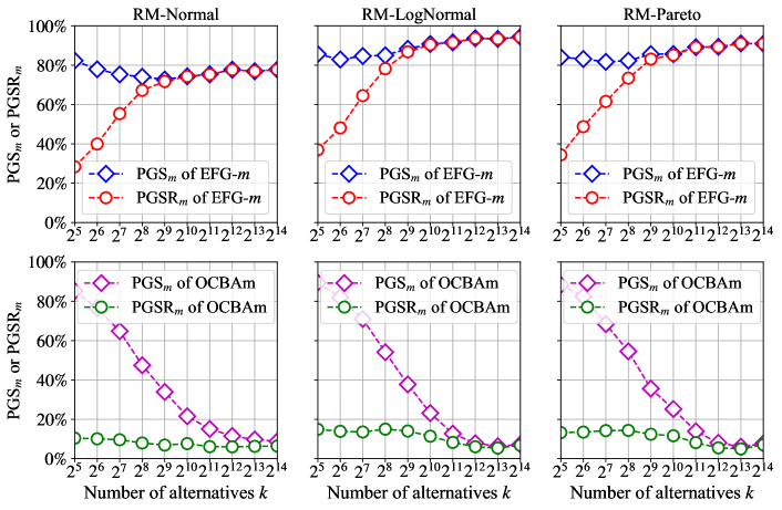
Figure 6: Free ranking effect of the EFG-$m$ procedure

7.3 Performance Improvement via Top-$\mathbf{M}$ Greedy Selection

This subsection will showcase the performance enhancement of the EFG-$M$ procedure with a top-$M$ greedy phase, which is introduced in Section 6.1, compared to the original EFG-$m$ procedure. For simplicity, we use the same three problem configurations and experiment settings as in Section 7.2, except setting the total sampling budget $B=100k$ for each $k$. Additionally, for the EFG-$M$ procedure, we set $M=2m$, which means that in each round of the greedy phase, the EFG-$M$ procedure will select and sample the current top-20 alternatives. Later we will investigate how the performance of the EFG-$M$ procedure varies with $M$. Then, for each problem configuration, we estimate and plot the PGS_m and PGSR_m of the EFG-$M$ procedure against different $k$ in Figure 7. To contrast the performance of the EFG-$M$ procedure with the EFG-$m$ procedure, we also include the PGS_m curves of the EFG-$m$ procedure in Figure 7.

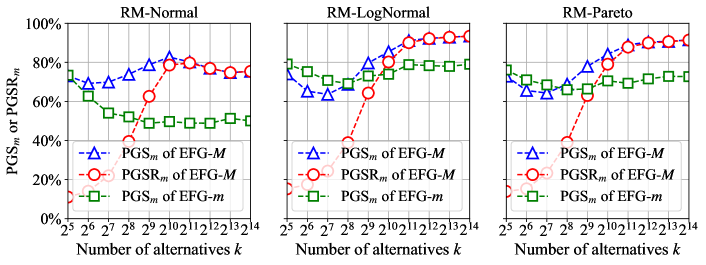
Figure 7: Performance enhancement through top-$M$ greedy selection

From Figure 7, we can draw several conclusions about the EFG-$M$ procedure. First, similar to the EFG-$m$ procedure, EFG-$M$ achieves the sample optimality for both the PGS_m and PGSR_m, showing consistent performance regardless of the normality of the simulation observations. Second, the EFG-$M$ procedure preserves the free ranking effect. Notably, when $k$ is large, the PGSR_m of the EFG-$M$ procedure coincides with its PGS_m. Third, the EFG-$M$ procedure demonstrates a marked improvement in performance over the EFG-$m$ procedure when $k$ is relatively large, particularly when $k\geq 2^{10}$. However, this is not the case when $k$ is small. In scenarios with smaller $k$ values, the performance of the EFG-$M$ procedure can fall short compared to the EFG-$m$ procedure, likely due to the small sampling budget $n_{g}k$ for the greedy phase at this scale. Consequently, selecting $M=2m$ alternatives in each round might be inefficient.

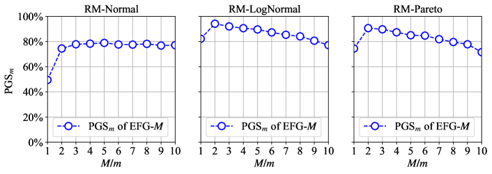
Figure 8: A comparison between the PGS_m of the EFG-$M$ procedure under different ${M/m}$

It is crucial to recognize the impact of the parameter $M$ on the EFG-$M$ procedure’s performance. To explore this, we fix $k=2^{14}$ and vary $M/m$ from 1 to 10 to analyze how changes in $M$ influence the PGS_m. Figure 8 shows the PGS_m curves of the EFG-$M$ procedure (notice that when $M/m=1$, EFG-$M$ becomes EFG-$m$). These curves show that the EFG-$M$ procedure’s performance may be insensitive to the choice of $M/m$. For the RM-Normal configuration, the curve is almost flat when $M/m\geq 2$; for the other configurations, as $M/m$ rises, the PGS_m of EFG-$M$ declines slowly and keeps its superiority over that of EFG-$m$ in a wide range. Besides, notice that for all tested configurations, the PGS_m peaks at $M/m=2$ or $M/m=3$. Based on this and our extensive tuning experience, we recommend setting $M$ to $2m$ or $3m$ to achieve near-optimal performance in practice.

7.4 Large-Scale Redundancy Allocation Problem

In this subsection, we compare our sample-optimal EFG-$m$ procedures with existing procedures in solving a practical large-scale redundancy allocation (RA) problem. A typical form of the RA problem involves a network of subsystems; the objective of the problem is to allocate a limited number of standby components to the subsystems to maximize the overall system reliability, commonly measured by the system lifetime. As a fundamental problem of reliability engineering, it attracts much research attention and has also been considered in the simulation literature; see, e.g., Chang and Kuo (2018).

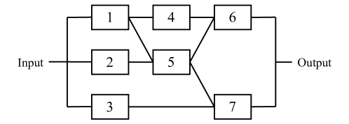
Figure 9: A communication network system

In our experiments, we adapt the communication network from Zhao and Liu (2003), which is shown in Figure 9. The system has 7 subsystems (nodes) and 6 paths. The lifetime of the system is determined by the most reliable path, that is, the path with the longest lifetime. However, for each path, P_j, $j=1,\dots,6$, the lifetime is determined by the most fragile subsystem in the path. Let $\phi_{i,k}$ represent the (random) lifetime of $k$-th component of subsystem $i$. Assuming the lifetime of different components to be independent, the total lifetime of subsystem $i$, if allocated to $x_{i}$ standby components in total, is $\sum_{k=1}^{x_{i}}\phi_{i,k}$. Then, for each alternative (i.e., feasible allocation scheme) $\mathbf{x}=[x_{1},x_{2}\ldots,x_{7}]\in\mathbb{N}^{7}_{+}$, its mean performance may be expressed as

$$\mu(\mathbf{x})= {\rm E}\left[\max_{j\in{1,\ldots,6}}\min_{i\in{P}_{j}}\sum_{k=1}^{x_{i}}\phi_{i,k}\right].$$ (29)

For simplicity, we assume that the standby components of different subsystems have the same price and the budget is only sufficient to purchase $L$ components. For a given $L$, our objective is to find a good subset of alternatives with $m=10$ and $\delta=0.1$ among all alternatives satisfying $\sum_{i=1}^{7}x_{i}=L$.

Following the reliability engineering literature, we let $\phi_{i,k}$ follow a lognormal distribution with common shape parameter $\mu_{i}$ and scale parameter $\sigma_{i}$ for the same subsystem $i$. In our experiments, we simply let $\mu_{1}=\mu_{4}=0.1$, $\mu_{2}=\mu_{4}=\mu_{6}=0.2$, $\mu_{3}=\mu_{7}=0.3$, and $\sigma_{1}=\cdots=\sigma_{7}=1.5$. Notice that the total number of alternatives $k$ is determined by the value of $L$. We consider several choices of $L$ to represent different problem scales. For each $L$, we estimate the mean performance of each alternative $i=1,\ldots,k$, which is expressed in Equation (29), based on 300,000 macro independent replications. We then summarize the information about the problem instances with different $L$ in Table 3.

Parameter $L$	Number of alt. $k$	$\mu_{1}$	$\mu_{m}$	$\mu_{k}$	Number of good alt. $|\mathcal{G}|$
13	1,716	4.315	4.049	1.795	23
14	3,432	4.779	4.567	1.800	18
16	11,440	5.944	5.703	1.800	18
19	50,388	7.844	7.545	1.800	16

Table 3: Information about the redundancy allocation problem instances

In the experiments, we evaluate the EFG-$m$, EFG-$M$, and EFG-$M$⁺ procedures using the problem instances detailed in Table 3, comparing them against the OCBAm and SAR procedures. For every problem instance, we set the total sampling budget $B=200k$. Then, we allocate 20% of this budget to the greedy phase for all our three procedures; for the EFG-$M$⁺ procedure, we allocate 10% of the budget to the seeding phase. Moreover, we let $M=2m$ for the EFG-$M$ procedure. Details on the implementation settings for the OCBAm and SAR procedures are provided in Section 12.1. We then estimate the PGS_m and PGSR_m of each procedure for every problem instance based on 200 independent macro replications, and summarize the results in Table 4.

$k$	1,716		3,432		1,1440		50,388
Measure	PGSm	PGSRm	PGSm	PGSRm	PGSm	PGSRm	PGSm	PGSRm
EFG-$m$	0.560	0.455	0.415	0.400	0.445	0.445	0.235	0.235
EFG-$M$	0.785	0.400	0.910	0.755	0.960	0.960	0.930	0.930
EFG-$M$+	0.905	0.490	0.965	0.775	1.000	1.000	1.000	1.000
SAR	0.770	0.235	0.825	0.510	0.855	0.835	0.875	0.875
OCBAm	0.000	0.000	0.000	0.000	0.000	0.000	0.010	0.000

Table 4: Estimated PGS_m and PGSR_m on the redundancy allocation problem instances

Table 4 offers insights into the performance of our EFG-$m$, EFG-$M$, and EFG-$M$⁺ procedures in solving large-scale OSS problems. First, the EFG-$m$ procedure, while being the simplest among the tested procedures, maintains a nonzero PGS_m across all tested problem instances, again demonstrating its sample optimality. In contrast, the OCBAm procedure fails to achieve this. Second, the EFG-$M$ procedure shows a clear advancement over the EFG-$m$ procedure, proving the effectiveness of using a top-$M$ greedy phase. Third, the EFG-$M$⁺ procedure outperforms both the EFG-$m$ and EFG-$M$ procedures in large-scale scenarios. Its exceptional performance underscores the importance of adaptive exploration budget allocation. Fourth, the EFG-$m$, EFG-$M$, and EFG-$M$⁺ procedures all demonstrate the free ranking effect; when $k$ is sufficiently large, their PGS_m coincide with their respective PGSR_m. Last, while the SAR procedure performs better than the original EFG-$m$ procedure, the EFG-$M$⁺ procedure consistently excels it for all five problem instances. These findings confirm the progression of improvements from EFG-$m$ through EFG-$M$ to EFG-$M$⁺, with each step introducing significant benefits; the EFG-$M$⁺ procedure emerges as especially powerful for achiving good selection and ranking in solving large-scale OSS problems.

8 Concluding Remarks

In this paper, we thoroughly investigate the large-scale OSS formulation for its better decision support in practice. We begin by defining the sample optimality in terms of the PGS_m, which denotes the probability of correctly selecting a good subset. Based on this definition, we propose the EFG-$m$ procedure, an interesting adaption of the standard EFG procedure, to achieve this sample optimality. From a boundary-crossing perspective, we derive a PGS_m lower bound for the EFG-$m$ procedure, from which we prove its sample optimality and consistency. Interestingly, the procedure is also shown to achieve the optimal sample complexity regarding various problem parameters. Furthermore, we consider rankings to provide decision makers with a deeper understanding into alternatives included in the selected subset. We for the first time introduce the concept of good ranking and define the PGSR_m. Surprisingly, we find that the EFG-$m$ procedure has the additional benefit of achieving a good ranking for free in the large-scale OSS problem. Again based on the boundary-crossing perspective, we prove the sample optimality and consistency of the EFG-$m$ procedure for the PGSR_m. Moreover, we extend the EFG-$m$ procedure to the EFG-$M$ and EFG-$M^{+}$ procedures to enhance practical applicability. Finally, a comprehensive numerical study validates our theoretical results and demonstrates the superior performance of our procedures in solving large-scale OSS problems.

To conclude this paper, we point out two potential directions worth of further investigation. First, numerical results in Section 7 demonstrate the robustness of our procedures in solving large-scale OSS problems with non-normal observations. This sets a theoretical challenge to rigorously establish the sample optimality of the procedures without relying on the normality assumption. Second, beyond the definition of “good subset” described in Section 2.1, there are other definitions, such as a subset consisting of only good alternatives that are within a small gap to the best alternative or a subset including at least one good alternative (Eckman and Henderson 2021). Our EFG-$m$ procedure may be directly applied to select such good subsets. Then, it would be interesting to investigate the EFG-$m$ procedure’s performance and prove the sample optimality in solving large-scale problems with these more diverse contexts.

E-Companion to
Sample-Optimal Large-Scale Optimal Subset Selection

9 Technical Supplements for Section 2

In this section, we will prove that for an OSS procedure, as long as $\limsup_{k\rightarrow\infty}|\mathcal{G}|<\infty$, the total sampling budget $B$ required to keep a positive PGS_m should increase at least linearly in the total number of alternatives $k$. This result serves as the theoretical basis for Definition 2.1. Inspired by Zhong and Hong (2022), we introduce the following assumptions on the budget allocation and selection behaviors of OSS procedures. Let $\mathcal{A}_{t}$ denote the set of alternatives having no observation when the procedure allocates the $t$-th observation. If the procedure allocates the $t$-th observation to an alternative in $\mathcal{A}_{t}$, then all alternatives in $\mathcal{A}_{t}$ have an equal probability of being selected. Let $\mathcal{A}$ denote the set of alternatives having no observation when the total sampling budget is exhausted. If $|\mathcal{A}|\geq m$ and the procedure chooses to select $m$ alternatives from $\mathcal{A}$, then all subsets of $\mathcal{A}$ containing $m$ alternatives have an equal probability of being selected.

Assumption 9 requires that allocating observations to alternatives with observations do not provide any information on the alternatives without any observations. Assumption 9 requires that after the total sampling budget is exhausted, if the procedure chooses to select $m$ alternatives from the set of alternatives without any observations, it can only randomly pick $m$ alternatives. Borrowing ideas from the proof of Theorem 1 in Zhong and Hong (2022), we may prove the following theorem.

Theorem 9.1

Suppose that $\limsup_{k\rightarrow\infty}|\mathcal{G}|<\infty$ and Assumptions 9 and 9 hold. Then, for any OSS procedure, if $\lim_{k\rightarrow\infty}B/k=0$,

$$\limsup_{k\rightarrow\infty}\mbox{PGS}_{m}=0.$$

Proof 9.2

Proof. We will prove the theorem by contradiction. Assume that

$$\limsup_{k\rightarrow\infty}\mbox{PGS}_{m}=\alpha$$ (30)

for some constant $\alpha\in(0,1]$. Let $g(k)=|\mathcal{G}|$ and $\bar{g}=\sup_{k\geq 1}g(k)$. Notice that since $\limsup_{k\rightarrow\infty}|\mathcal{G}|<\infty$, $\bar{g}<\infty$. Then, let $c_{\alpha}=1-\sqrt[\bar{g}]{1-{\alpha}/{4}}$. Furthermore, since $\lim_{k\rightarrow\infty}B/k=0$, there must exist a finite $K_{0}$ such that as long as $k\geq K_{0}$, $B\leq c_{\alpha}k$. In the following, we consider $k\geq\max\left\{{\bar{g}}/(1-c_{\alpha}),K_{0}\right\}$. For an OSS procedure, the PGS_m, i.e., the probability that the selected subset $\mathcal{S}$ includes $m$ good alternatives can be decomposed as

$$\mbox{PGS}_{m}= \Pr\left\{\{\mathcal{S}\subseteq\mathcal{G}\}\cap\{\mathcal{G}\text{ has at least one obs.}\}\right\}+\Pr\left\{\{\mathcal{S}\subseteq\mathcal{G}\}\cap\{\mathcal{G}\text{ has no obs.}\}\right\}$$ (31)

$$\leq\Pr\left\{\mathcal{G}\text{ has at least one obs.}\right\}+\Pr\left\{\mathcal{G}\text{ has no obs.}\right\},$$

where $\{\mathcal{G}\text{ has at least one obs.}\}$ means that there is at least one good alternative has observations, while $\{\mathcal{G}\text{ has no obs.}\}$ means that none of the good alternatives has any observation. We then analyze the two probabilities on the right-hand side (RHS) of Equation (31) separately.

Let’s denote the event that the procedure allocates the $t$-th observation to an alternative not belonging to $\mathcal{G}$ as $\Omega_{t}$. Then, for the first term on the RHS of Equation (31), we have

$$\Pr\left\{\mathcal{G}\text{ has at least one obs.}\right\} \leq 1-\Pr\left\{\bigcap_{t=1}^{B}\Omega_{t}\right\}=1-\Pr\left\{\Omega_{1}\right\}\times\prod_{t=2}^{B}\Pr\left\{\Omega_{t}\mid\Omega_{1},\ldots,\Omega_{t-1}\right\}.\quad\quad\quad\quad$$ (32)

Under Assumption 9, we may know

$$\Pr\left\{\Omega_{1}\right\}\geq\frac{k-g(k)}{k}\text{ and }\Pr\left\{\Omega_{t}\mid\Omega_{1},\ldots,\Omega_{t-1}\right\}\geq\frac{k-t+1-g(k)}{k-t+1}\quad\forall t\geq 2,$$ (33)

because there are at least $k-(t-1)$ alternatives having no any observation when the procedure allocates the $t$-th observation. Combining Equations (32) and (33), we further derive

$$\Pr\left\{\mathcal{G}\text{ has at least one obs.}\right\} \leq 1-\frac{k-g(k)}{k}\cdot\frac{k-1-g(k)}{k-1}\cdot\cdots\cdot\frac{k-B+1-g(k)}{k-B+1}$$ (34)

$$\leq 1-\frac{k-\bar{g}}{k}\cdot\frac{k-1-\bar{g}}{k-1}\cdot\cdots\cdot\frac{k-c_{\alpha}k+1-\bar{g}}{k-c_{\alpha}k+1}$$

$$= 1-\prod_{i=1}^{\bar{g}}\frac{k-c_{\alpha}k-(i-1)}{k-(i-1)}$$

$$\leq 1-\left(\frac{k-c_{\alpha}k-(\bar{g}-1)}{k-(\bar{g}-1)}\right)^{\bar{g}}=:f_{1}(k;c_{\alpha},\bar{g}),\qquad\qquad\qquad$$

where the second inequality holds because $g(k)\leq\bar{g}$ and $B\leq c_{\alpha}k$, and the last inequality holds because $k\geq{\bar{g}}/(1-c_{\alpha})$.

For the second term on the RHS of Equation (31), notice that since $k\geq\bar{g}/(1-c_{\alpha})$, there are at least $k-c_{\alpha}k\geq\bar{g}\geq m$ alternatives having no observation. Then, according to Assumption 9,

$$\Pr\left\{\{\mathcal{G}\text{ has no obs.}\}\right\} = \Pr\left\{\{\text{at least }k-c_{\alpha}k\text{ alternatives has no obs.}\}\cap\{\mathcal{G}\text{ has no obs.}\}\right\}$$ (35)

$$\leq \frac{1}{\tbinom{k-c_{\alpha}k}{g(k)}}\leq\frac{g(k)}{k-c_{\alpha}k}\leq\frac{\bar{g}}{k-c_{\alpha}k}=:f_{2}(k;c_{\alpha},\bar{g}).$$

Combining Equations (34) and (35) and the fact that $\lim_{k\to\infty}f_{1}(k;c_{\alpha},\bar{g})=1-(1-c_{\alpha})^{\bar{g}}=\alpha/4$ and $\lim_{k\to\infty}f_{2}(k;c_{\alpha},\bar{g})=0$, there must exist a finite $K_{1}$ such that when $k\geq K_{1}$,

$$\mbox{PGS}_{m}\leq f_{1}(k;c_{\alpha},\bar{g})+f_{2}(k;c_{\alpha},\bar{g})\leq\frac{\alpha}{2},$$

which contradicts with Equation (30). The conclusion of interest is now proved.

10 Technical Supplements for Section 4

10.1 Proof of Theorem 4.3

The proof presented here follows the proof of Theorem 3 in Li et al. (2024). To ensure self-containment and clarity, we provide below a detailed argument.

Proof 10.1

Proof of Theorem 4.3: Given a total sampling budget $B=(n_{0}+n_{g})k$, the PGS_m lower bound of the EFG-$m$ procedure stated in Equation (15) can be rewritten as

$$\mbox{PGS}_{m} \geq \Pr\left\{\frac{n_{g}}{m}+n_{0}\geq\frac{1}{k}\sum_{j\in\mathcal{G}}\argmin_{n\geq n_{0}}\bar{X}_{j}(n)+\frac{1}{k}\sum_{i\in\mathcal{K}\setminus\mathcal{G}}N_{i}\left(\bar{X}^{*}_{(m)};n_{0}\right)\right\}.$$

Since $n_{g}>m\left[C(\delta/\bar{\gamma};n_{0})-n_{0}\right]$, we can arbitrarily fix a constant $\lambda$ such that $0<\lambda<n_{g}/m+n_{0}-C(\delta/\bar{\sigma};n_{0})$. Then, we may select a positive $\delta_{\lambda}\in(0,\delta)$ such that

$$C\left(\frac{\delta-\delta_{\lambda}}{\bar{\sigma}};n_{0}\right)=n_{g}/m+n_{0}-\lambda>0.$$ (36)

The existence of such $\delta_{\gamma}$ can be ensured due to that by the virtue of definition, $C(x;n_{0})$ is a continuous and monotonically decreasing function on $x\in(0,\infty)$, and $C(x;n_{0})\to 0$ as $x\to\infty$ for any fixed $n_{0}$. For the given $\gamma$, we may further derive the PGS lower bound in Equation (10.1) as

$$\mbox{PGS}_{m}\geq \Pr\Bigg{\{}\Bigg{\{}\frac{n_{g}}{m}+n_{0}\geq\frac{1}{k}\sum_{j\in\mathcal{G}}\argmin_{n\geq n_{0}}\bar{X}_{j}(n)+\frac{1}{k}\sum_{i\in\mathcal{K}\setminus\mathcal{G}}N_{i}\left(X^{*}_{(m)};n_{0}\right)\Bigg{\}}\qquad\qquad\qquad\qquad$$ (37)

$$\qquad\qquad\qquad\qquad\qquad\qquad\qquad\qquad\qquad\qquad\qquad\cap\left\{\bar{X}^{*}_{(m)}\geq\mu_{m}-\delta_{\gamma}\right\}\Biggr{\}}.$$

Now we proceed to study the limiting behavior of the PGS_m bound presented in Equation (37). Firstly, according to Argument 1, we have $\sum_{j\in\mathcal{G}}\argmin_{n\geq n_{0}}\bar{X}_{j}(n)<\infty$ almost surely. This indicates

$$\Pr\left\{\sum_{j\in\mathcal{G}}\argmin_{n\geq n_{0}}\bar{X}_{j}(n)\leq\frac{\lambda}{2}\right\}\nearrow\Pr\left\{\sum_{j\in\mathcal{G}}\argmin_{n\geq n_{0}}\bar{X}_{j}(n)<\infty\right\}=1,\mbox{ as }k\to\infty.$$ (38)

Additionally, Argument 2 states that, under the condition $\bar{X}^{*}_{(m)}\geq\mu_{m}-\delta_{\gamma}$,

$$\liminf_{k\to\infty}\ \frac{1}{k}\sum_{i\in\mathcal{K}\setminus\mathcal{G}}N_{i}\left(X^{*}_{(m)};n_{0}\right)\leq\limsup_{k\to\infty}\ \frac{1}{k}\sum_{i\in\mathcal{K}\setminus\mathcal{G}}N_{i}\left(X^{*}_{(m)};n_{0}\right)\leq C\left(\frac{\delta-\delta_{\gamma}}{\bar{\sigma}};n_{0}\right),\mbox{ almost surely}.$$

Therefore, it is clear that, for the given $\lambda$,

$$\liminf_{k\to\infty}\ \Pr\left\{\frac{1}{k}\sum_{i\in\mathcal{K}\setminus\mathcal{G}}N_{i}\left(X^{*}_{(m)};n_{0}\right)\leq C\left(\frac{\delta-\delta_{\gamma}}{\bar{\sigma}};n_{0}\right)+\frac{\lambda}{2}\right\}=1.$$ (39)

For the ease of presentation, we define two events

$$\Omega_{\argmin}=\left\{\frac{1}{k}\sum_{j\in\mathcal{G}}\argmin_{n\geq n_{0}}\bar{X}_{j}(n)\leq\frac{\lambda}{2}\right\},\mbox{ and }\Omega_{N}=\left\{\frac{1}{k}\sum_{i\in\mathcal{K}\setminus\mathcal{G}}N_{i}\left(X^{*}_{(m)};n_{0}\right)\leq C\left(\frac{\delta-\delta_{\gamma}}{\bar{\sigma}};n_{0}\right)+\frac{\lambda}{2}\right\}.$$

By Equations (38) and (39), they satisfy

$$\lim_{k\to\infty}\Pr\{\Omega_{\argmin}\}=1,\mbox{ and }\liminf_{k\to\infty}\ \Pr\{\Omega_{N}|\bar{X}^{*}_{(m)}\geq\mu_{m}-\delta_{\gamma}\}=1.$$ (40)

Now we are ready to study the limiting behavior of PGS_m. Notice that Equation (37) can be further reformulated as

$$\mbox{PGS}_{m} \geq \Pr\Bigg{\{}\Bigg{\{}\frac{n_{g}}{m}+n_{0}\geq\frac{1}{k}\sum_{j\in\mathcal{G}}\argmin_{n\geq n_{0}}\bar{X}_{j}(n)+\frac{1}{k}\sum_{i\in\mathcal{K}\setminus\mathcal{G}}N_{i}\left(\bar{X}^{*}_{(m)};n_{0}\right)\Bigg{\}}\cap\{\bar{X}^{*}_{(m)}\geq\mu_{m}-\delta_{\gamma}\}\Bigg{\}}\qquad$$ (41)

$$\geq \Pr\Bigg{\{}\Bigg{\{}\frac{n_{g}}{m}+n_{0}\geq\frac{1}{k}\sum_{j\in\mathcal{G}}\argmin_{n\geq n_{0}}\bar{X}_{j}(n)+\frac{1}{k}\sum_{i\in\mathcal{K}\setminus\mathcal{G}}N_{i}\left(\bar{X}^{*}_{(m)};n_{0}\right)\Bigg{\}}$$

$$\qquad\qquad\qquad\qquad\qquad\qquad\qquad\quad\cap\,\Omega_{\argmin}\cap\Omega_{N}\cap\left\{\bar{X}^{*}_{(m)}\geq\mu_{m}-\delta_{\gamma}\right\}\Bigg{\}}$$

$$\geq \Pr\left\{\left\{\frac{n_{g}}{m}+n_{0}\geq\frac{\lambda}{2}+C\left(\frac{\delta-\delta_{\gamma}}{\bar{\sigma}};n_{0}\right)+\frac{\lambda}{2}\right\}\cap\Omega_{\argmin}\cap\Omega_{N}\cap\{\bar{X}^{*}_{(m)}\geq\mu_{m}-\delta_{\gamma}\}\right\}$$

$$= \Pr\left\{\Omega_{\argmin}\cap\Omega_{N}\cap\{\bar{X}^{*}_{(m)}\geq\mu_{m}-\delta_{\gamma}\}\right\},$$

where the second inequality holds because additional condition $\Omega_{\argmin}\cap\Omega_{N}$ is imposed, the third inequality holds by the definition of $\Omega_{\argmin}$ and $\Omega_{N}$, and the last equality holds from the choice of $\delta_{\lambda}$ in Equation (36). By using the Bonferroni’s inequality in Equation (41), we may further have

$$\mbox{PGS}_{m} \geq \Pr\left\{\Omega_{N}\cap\{\bar{X}^{*}_{(m)}\geq\mu_{m}-\delta_{\gamma}\}\right\}-\Pr\left\{\Omega_{\argmin}^{c}\right\}$$

$$= \Pr\left\{\Omega_{N}|\bar{X}^{*}_{(m)}\geq\mu_{m}-\delta_{\gamma}\right\}\Pr\{\bar{X}^{*}_{(m)}\geq\mu_{m}-\delta_{\gamma}\}-\Pr\left\{\Omega_{\argmin}^{c}\right\}.$$

Then, according to Equation (40),

$$\liminf_{k\to\infty}\mbox{PGS}_{m} \geq \ \Pr\{\bar{X}^{*}_{(m)}\geq\mu_{m}-\delta_{\gamma}\}\liminf_{k\to\infty}\ \Pr\left\{\Omega_{N}|\bar{X}^{*}_{(m)}\geq\mu_{m}-\delta_{\gamma}\right\}-\limsup_{k\to\infty}\Pr\left\{\Omega_{\argmin}^{c}\right\}$$ (42)

$$= \ \Pr\{\bar{X}^{*}_{(m)}\geq\mu_{m}-\delta_{\gamma}\}.$$

Lastly, by the definition of $\delta_{\gamma}$, we can see that $\delta_{\lambda}\to\delta_{0}$ as $\lambda\to 0$. Meanwhile, it is important to notice that Equation (42) is true for any $\lambda\in(0,n_{g}/m+n_{0}-C(\delta/\bar{\sigma};n_{0}))$ and its corresponding choice of $\delta_{\lambda}$. Therefore, we can let $\lambda\to 0$ in Equation (42) to further get

$$\liminf_{k\to\infty}\mbox{PGS}_{m} \geq \Pr\{\bar{X}^{*}_{(m)}\geq\mu_{m}-\delta_{0}\}.$$

This concludes the proof of the theorem.

10.2 Proof of Lemma 4.4

To prove the lemma, we first prepare the following lemma.

Lemma 10.2

Let $\Phi(x)$ be the cumulative distribution function of the standard normal distribution. Then, for any $x>0$,

$$1-\Phi(x)\leq\exp\left(-\frac{x^{2}}{2}\right).$$

Proof 10.3

Proof of Lemma 4.4:Let $B(t)$ denote a standard Brownian motion with zero drift and volatility one. Notice that the running average process $\{n(\bar{X}_{j}(n)-\mu_{j})/\sigma_{j}:n=n_{0},n_{0}+1,\dots\}$ has the same joint distribution with the discrete-time process $\{B(t):t=n_{0},n_{0}+1,\dots\}$. Then,

$$\Pr\left\{\min_{n\geq n_{0}}\bar{X}_{j}(n)>\mu_{j}-\delta_{0}\right\} = \Pr\left\{\forall\,n_{0}\leq n<\infty,\bar{X}_{j}(n)>\mu_{j}-\delta_{0}\right\}$$ (43)

$$= \Pr\left\{\forall\,n_{0}\leq n<\infty,n(\bar{X}_{j}(n)-\mu_{j})/\sigma_{j}>-n\delta_{0}/\sigma_{j}\right\}$$

$$= \Pr\left\{\forall\,n_{0}\leq n<\infty,B(n)>-n\delta_{0}/\sigma_{j}\right\}$$

$$\geq \Pr\left\{\forall\,n_{0}\leq t<\infty,B(t)>-t\delta_{0}/\sigma_{j}\right\}.$$

By the time-inversion property of standard Brownian motion $\{B(t):t\geq 0\}$, the new stochastic process $\{\tilde{B}(t):t\geq 0\}$ defined as $\tilde{B}(t):=tB(1/t)$ for $t>0$ and $\tilde{B}(0)=0$ for $t=0$ is also a standard Brownian motion. Therefore, we may further derive Equation (43) as

$$\Pr\left\{\,\min_{n\geq n_{0}}\bar{X}_{j}(n)>\mu_{j}-\delta_{0}\right\} \geq \Pr\left\{\,\forall\,n_{0}\leq t<\infty,B(t)>-t\delta_{0}/\sigma_{j}\right\}$$ (44)

$$= \Pr\left\{\,\forall\,n_{0}\leq t<\infty,s=1/t,sB(1/s)>-\delta_{0}/\sigma_{j}\right\}$$

$$= \Pr\left\{\,\forall\,0<s\leq 1/n_{0},\tilde{B}(s)>-\delta_{0}/\sigma_{j}\right\}$$

$$= \Pr\left\{\inf_{0\leq s\leq 1/n_{0}}\tilde{B}(s)>-\delta_{0}\sigma_{j}\right\}$$

$$= \Pr\left\{\sup_{0\leq s\leq 1/n_{0}}\tilde{B}(s)\leq\delta_{0}/\sigma_{j}\right\},$$

where the last equality holds from the space symmetry of standard Brownian motion. Furthermore, considering the reflection principle of standard Brownian motion, we see that

$$\Pr\left\{\sup_{0\leq s\leq 1/n_{0}}\tilde{B}(s)\geq\delta_{0}/\sigma_{j}\right\}=2\Pr\{\tilde{B}(1/n_{0})\geq\delta_{0}/\sigma_{j}\}=2\left(1-\Phi\left(\frac{\sqrt{n_{0}}\delta_{0}}{\sigma_{j}}\right)\right).\quad\quad$$ (45)

Plugging Equation (45) into Equation (44) results in

$$\Pr\left\{\,\min_{n\geq n_{0}}\bar{X}_{j}(n)>\mu_{j}-\delta_{0}\right\}\geq 1-2\left(1-\Phi\left(\frac{\sqrt{n_{0}}\delta_{0}}{\sigma_{j}}\right)\right)\geq 1-2\left(1-\Phi\left(\frac{\sqrt{n_{0}}\delta_{0}}{\bar{\sigma}}\right)\right),\quad\quad$$ (46)

where the the last inequality arises from Assumption 4 Then, by Lemma 10.2, it is straightforward to draw the desired conclusion.

10.3 Proof of Theorem 4.5

To prove the theorem, we first prepare the following lemma.

Lemma 10.4 (Lemma 6 of Li et al. 2024)

For any positive constant $b>0$, there exist positive constants $\beta$ and $\kappa$ such that $C\left(b;n_{0}\right)-n_{0}\leq\beta e^{-\kappa n_{0}}$, where $\kappa=\frac{b^{2}}{2}$ and $\beta=\left(1-e^{-\kappa}\right)^{-1}$.

Proof 10.5

Proof of Theorem 4.5: It follows from Lemma 10.4 and the choice of $n_{g}$ that

$$n_{g}=m\left[C\left(\frac{\delta}{2\bar{\sigma}};n_{0}\right)-n_{0}\right]\leq m\beta\exp\left(-\frac{\delta^{2}}{8\bar{\sigma}^{2}}n_{0}\right),$$ (47)

where $\beta=\left(1-e^{-\frac{\delta^{2}}{8\bar{\sigma}^{2}}}\right)^{-1}$. By the choice of $n_{0}$, namely, $n_{0}=\frac{8\bar{\sigma}^{2}}{\delta^{2}}\log\frac{2m}{\delta}$, we further derive Equation (47) as

$$n_{g}\leq m\beta\exp\left(-\frac{\delta^{2}}{8\bar{\sigma}^{2}}n_{0}\right)=\frac{\beta\alpha}{2}.$$ (48)

Next, notice that $e^{-x}\leq 1/(1+x)$ for any $x>0$, so we have,

$$\beta=\left(1-e^{-\frac{\delta^{2}}{8\bar{\sigma}^{2}}}\right)^{-1}\leq\left(1-\frac{1}{\frac{\delta^{2}}{8\bar{\sigma}^{2}}+1}\right)^{-1}=\frac{\frac{\delta^{2}}{8\bar{\sigma}^{2}}+1}{\frac{\delta^{2}}{8\bar{\sigma}^{2}}}=1+\frac{8\bar{\sigma}^{2}}{\delta^{2}}.$$ (49)

Combining Equation (48) and Equation (49) leads to the conclusion.

10.4 Proof of Lemma 5.2

Proof 10.6

Proof. In this proof, we first demonstrate that $L_{\mathcal{G}}^{j}(\delta/2;n_{0})=\sup\left\{n\geq n_{0}:|\bar{X}_{j}(n)-\mu_{j}|\geq\delta/2\right\}$ is finite almost surely for any alternative $j\in\mathcal{G}$. For any sufficiently large integer $M>n_{0}$, we have

$$\Pr\left\{L_{\mathcal{G}}^{j}(\delta/2;n_{0})<M\right\} = \Pr\left\{\forall\,n\geq M,\,|\bar{X}_{j}(n)-\mu_{j}|\leq\delta/2\right\}$$ (50)

$$= \Pr\left\{\min_{n\geq M}\bar{X}_{j}(n)\geq\mu_{j}-\delta/2,\max_{n\geq M}\bar{X}_{j}(n)\leq\mu_{j}+\delta/2\right\}$$

$$\geq \Pr\left\{\min_{n\geq M}\bar{X}_{j}(n)\geq\mu_{j}-\delta/2\right\}-\Pr\left\{\max_{n\geq M}\bar{X}_{j}(n)\geq\mu_{j}+\delta/2\right\},\quad\quad\quad\quad\quad$$

where the inequality holds because $\Pr\{A\cap B\}=\Pr\{A\}-\Pr\{A\cap B^{c}\}\geq\Pr\{A\}-\Pr\{B^{c}\}$ for any two events $A$ and $B$.

Notice that the second term in Equation (50) satisfies

$$\Pr\left\{\max_{n\geq M}\bar{X}_{j}(n)\geq\mu_{j}+\delta/2\right\} = 1-\Pr\left\{\max_{n\geq M}\bar{X}_{j}(n)\leq\mu_{j}+\delta/2\right\}$$ (51)

$$= 1-\Pr\left\{\max_{n\geq M}\,(\bar{X}_{j}(n)-\mu_{j})\leq\delta/2\right\}$$

$$= 1-\Pr\left\{\min_{n\geq M}\,(\bar{X}_{j}(n)-\mu_{j})\geq-\delta/2\right\}$$

$$= 1-\Pr\left\{\min_{n\geq M}\,\bar{X}_{j}(n)\geq\mu_{j}-\delta/2\right\},$$

where the third equality holds because $\{\bar{X}_{j}(n)-\mu_{j}:n\geq 1\}$ and $\{-(\bar{X}_{j}(n)-\mu_{j}):n\geq 1\}$ have the same joint probability density function. Plugging Equation (51) into (50) leads to

$$\Pr\left\{L_{\mathcal{G}}^{j}(\delta/2;n_{0})<M\right\}\geq 2\Pr\left\{\min_{n\geq M}\,\bar{X}_{j}(n)\geq\mu_{j}-\delta/2\right\}-1.$$

Then, similar to Equation (46) in the proof of Lemma 4.4, we have

$$\Pr\left\{\,\min_{n\geq M}\bar{X}_{j}(n)>\mu_{j}-\delta/2\right\}\geq 1-2\left(1-\Phi\left(\frac{\sqrt{M}\delta}{2\sigma_{i}}\right)\right),$$

where $\Phi(\cdot)$ denotes the cumulative distribution function of a standard normal distribution. Therefore,

$$\Pr\left\{L_{\mathcal{G}}^{j}(\delta/2;n_{0})<M\right\}\geq 1-4\left(1-\Phi\left(\frac{\sqrt{M}\delta}{2\sigma_{i}}\right)\right)$$

Letting $M\to\infty$ in the equation above, we may conclude that

$$\Pr\left\{L_{\mathcal{G}}^{j}(\delta/2;n_{0})<\infty\right\}=1.$$ (52)

Now we move to demonstrate the desired conclusion. Observe that

$$\limsup_{k\rightarrow\infty}\frac{1}{k}\sum\limits_{j\in\mathcal{G}^{\prime}}\left(L_{\mathcal{G}^{\prime}}^{j}(\delta/2;n_{0})-\argmin_{n\geq n_{0}}\bar{X}_{j}(n)\right)^{+}$$

$$\leq \limsup_{k\rightarrow\infty}\frac{1}{k}\sum\limits_{j\in\mathcal{G}}\left(L_{\mathcal{G}}^{j}(\delta/2;n_{0})-\argmin_{n\geq n_{0}}\bar{X}_{j}(n)\right)^{+}\quad(\mbox{because }\mathcal{G}^{\prime}\subseteq\mathcal{G})$$

$$\leq \limsup_{k\rightarrow\infty}\frac{1}{k}\sum\limits_{j\in\mathcal{G}}L_{\mathcal{G}}^{j}(\delta/2;n_{0})+\limsup_{k\rightarrow\infty}\frac{1}{k}\sum\limits_{j\in\mathcal{G}}\argmin_{n\geq n_{0}}\bar{X}_{j}(n)$$

$$= 0,\mbox{ almost surely.}$$

The last equality holds from Equation (52) and Lemma 4.1. The proof is completed.

10.5 Proof of Theorem 5.3

Proof 10.7

Proof. Given the similarity between the lower bounds for PGS_m and PGSR_m as listed in Equations (14) and (24), we may follow the proofs of Theorem 4.3 and Theorem 4.5 to complete this proof, by specifically dealing with the additional term $\sum_{j\in\mathcal{G}^{\prime}}\left(L_{\mathcal{G}^{\prime}}^{j}(\delta/2;n_{0})-\argmin_{n\geq n_{0}}\bar{X}_{j}(n)\right)^{+}$ in Equation (24).

When the total sampling budget $B=(n_{0}+n_{g})k$, the PGSR_m of the EFG-$m$ procedure in Equation (24) can be rewritten as

$$\mbox{PGSR}_{m} \geq \Pr\left\{\frac{n_{g}}{m}+n_{0}\geq\frac{1}{k}\left[\sum\limits_{j\in\mathcal{G}^{\prime}}\left(L_{\mathcal{G}^{\prime}}^{j}(\delta/2;n_{0})-\underset{n\geq n_{0}}{\argmin}\bar{X}_{j}(n)\right)^{+}\right.\right.$$ (53)

$$\qquad\qquad\qquad\qquad\qquad\left.\left.+\sum\limits_{l\in\mathcal{G}}\underset{n\geq n_{0}}{\argmin}\bar{X}_{l}(n)+\sum\limits_{i\in\mathcal{K}\setminus\mathcal{G}}N_{i}(\bar{X}^{*}_{(m)};n_{0})\right]\right\}.\qquad$$

Inspired by Equation (36), we can arbitrarily fix a constant $\lambda\in(0,n_{g}/m+n_{0}-C(\delta/\bar{\sigma};n_{0}))$ and accordingly set $\delta_{\lambda}\in(0,\delta)$ such that

$$C\left(\frac{\delta-\delta_{\lambda}}{\bar{\sigma}};n_{0}\right)=n_{g}/m+n_{0}-\lambda>0.$$ (54)

Meanwhile, for the ease of presentation, we define the events

$$\Omega_{L}=\ \left\{\frac{1}{k}\sum\limits_{j\in\mathcal{G}^{\prime}}\left(L_{\mathcal{G}^{\prime}}^{j}(\delta/2;n_{0})-\underset{n\geq n_{0}}{\argmin}\,\bar{X}_{j}(n)\right)^{+}\leq\frac{\lambda}{3}\right\},\,\Omega_{\argmin}=\ \left\{\frac{1}{k}\sum\limits_{l\in\mathcal{G}}\underset{n\geq n_{0}}{\argmin}\,\bar{X}_{l}(n)\leq\frac{\lambda}{3}\right\},$$

and for the chosen $\delta_{\gamma}$,

$$\Omega_{N}=\left\{\frac{1}{k}\sum_{i\in\mathcal{K}\setminus\mathcal{G}}N_{i}\left(X^{*}_{(m)};n_{0}\right)\leq C\left(\frac{\delta-\delta_{\gamma}}{\bar{\sigma}};n_{0}\right)+\frac{\lambda}{3}\right\}.$$

Then, the PGS_m lower bound in Equation (53) can be further derived as

$$\mbox{PGSR}_{m} \geq \Pr\Bigg{\{}\Bigg{\{}\frac{n_{g}}{m}+n_{0}\geq\frac{1}{k}\Bigg{[}\sum\limits_{j\in\mathcal{G}^{\prime}}\left(L_{\mathcal{G}^{\prime}}^{j}(\delta/2;n_{0})-\underset{n\geq n_{0}}{\argmin}\bar{X}_{j}(n)\right)^{+}$$ (55)

$$\qquad\qquad\qquad\qquad+\sum\limits_{l\in\mathcal{G}}\underset{n\geq n_{0}}{\argmin}\bar{X}_{l}(n)+\sum\limits_{i\in\mathcal{K}\setminus\mathcal{G}}N_{i}(\bar{X}^{*}_{(m)};n_{0})\Bigg{]}\Bigg{\}}\cap\,\Omega_{L}\cap\,\Omega_{\argmin}\cap\,\Omega_{N}\Bigg{\}}$$

$$\geq \Pr\left\{\left\{\frac{n_{g}}{m}+n_{0}\geq C\left(\frac{\delta-\delta_{\gamma}}{\bar{\sigma}};n_{0}\right)+\lambda\right\}\cap\,\Omega_{L}\cap\,\Omega_{\argmin}\cap\,\Omega_{N}\right\}$$

$$= \Pr\left\{\Omega_{L}\cap\,\Omega_{\argmin}\cap\,\Omega_{N}\right\}$$

$$\geq \Pr\left\{\Omega_{N}\right\}-\Pr\left\{\Omega_{\argmin}^{c}\right\}-\Pr\left\{\Omega_{L}^{c}\right\},$$

$$\geq \Pr\left\{\Omega_{N}\mid\{\bar{X}^{*}_{(m)}\geq\mu_{m}-\delta_{\gamma}\}\right\}\Pr\left\{\bar{X}^{*}_{(m)}\geq\mu_{m}-\delta_{\gamma}\right\}-\Pr\left\{\Omega_{\argmin}^{c}\right\}-\Pr\left\{\Omega_{L}^{c}\right\},$$

where the second inequality holds because of the definitions of the events $\Omega_{L}$, $\Omega_{N}$ and $\Omega_{\argmin}$, the first equality holds due to Equation (54), and the third inequality holds because of the Bonferroni’s inequality. Notice that Equation (42) gives the limiting behavior of the first two probability terms in (55). More specifically, we have

$$\liminf_{k\to\infty}\mbox{PGSR}_{m}\geq\Pr\left\{\bar{X}^{*}_{(m)}\geq\mu_{m}-\delta_{\gamma}\right\}-\limsup_{k\to\infty}\Pr\left\{\Omega_{L}^{c}\right\}.$$

Then, it readily follows from Lemma 5.2 that $\limsup_{k\to\infty}\Pr\left\{\Omega_{L}^{c}\right\}=0$. As the inequality above holds for any $\lambda\in(0,n_{g}/m+n_{0}-C(\delta/\bar{\sigma};n_{0}))$, by letting $\lambda\to 0$, we further have $\liminf_{k\to\infty}\mbox{PGSR}_{m}\geq\Pr\left\{\bar{X}^{*}_{(m)}\geq\mu_{m}-\delta_{0}\right\}$. The sample optimality is now proved.

For the consistency, notice that PGSR_m shares the same limiting lower bound as the PGS_m. Then, following exactly the same logic in the proof of Theorem 4.5, it is straightforward to show that the EFG-$m$ procedure is also consistent in terms of PGSR_m. The proof is completed.

11 Supplements to Section 6

11.1 The EFG-$M$⁺ Procedure

As introduced in Section 6.1, to further enhance the EFG-$M$ procedure, we add a seeding phase before the exploration phase and obtain the EFG-$M^{+}$ procedure. Specifically, the EFG-$M^{+}$ procedure consists of three phases: the seeding phase, the exploration phase, and the top-$M$ greedy phase. In the seeding phase, the procedure first allocates an equal number of $n_{sd}$ observations to every alternative and then compute its sample mean; based on the sample information, the procedure then ranks the alternatives in descending order and divides the ranked alternatives into $G$ disjoint groups so that group 1 includes the fewest alternatives, group 2 doubles group 1, group 3 doubles group 2, and so on so force. Subsequently, in the exploration phase, the procedure equally allocates the exploration budget $n_{0}k$ to the $G$ groups and for each group, it equally allocates the group budget to the alternatives inside the group. By doing so, the procedure will allocate more budget to the alternatives in top groups and that are likely to have top mean performances, which introduces adaptation to exploration. Then, in the top-$M$ greedy phase, the procedure selects the current top-$M$ alternatives at each round. Finally, it delivers the top-$m$ alternatives after the total sampling budget is exhausted. See Procedure 3 for a detailed description of the procedure. Notice that in the EFG-$M^{+}$ procedure, the number of groups $G$ is a use-specified parameter. In our experiments, we let $G=\left\lfloor\log_{2}(k/m)\right\rfloor$ to ensure that each group includes at least one alternative. Numerical results in Section 7.4 show that this procedure performs very well in solving large-scale OSS problems.

Input: $k$ alternatives $X_{1},\ldots,X_{k}$, the total sampling budget $B=(n_{sd}+n_{0}+n_{g})k$, $n_{sd}$, $n_{0}$, $n_{g}$, $m$, $M$ and the total number of groups $G$

1

2for $i=1$ to $k$  do // Seeding Phase

3       take $n_{sd}$ observations $x_{i1},\ldots,x_{in_{sd}}$ from alternative $X_{i}$;

4       set $\bar{X}^{sd}_{i}=\frac{1}{n_{sd}}\sum_{j=1}^{n_{sd}}x_{ij}$;

5      

6 end for

7according to $\bar{X}^{sd}_{i}$, sort the alternatives in descending order as $\{(1),(2),\ldots,(k)\}$;

8

9let $I^{r}$ denote the group of alternatives for $r=1,\ldots,G$. Set $\Delta=2^{G}-1$. Then, let $I^{1}=\{(1),(2),\ldots,(\lfloor k/\Delta\rfloor)\}$, $I^{r}=\{(\lfloor k2^{r-2}/\Delta\rfloor+1),\ldots,(\lfloor k2^{r-1}/\Delta\rfloor)\}$ for $r=2,\ldots,G-1$, and $I^{G}=\{(\lfloor k2^{G-2}/\Delta\rfloor+1),\ldots,(k)\}$;

10

11for $r=1$ to $G$ do // Exploration Phase

12       set the sample size $n^{r}=\left\lfloor\frac{n_{0}(2^{G}-1)}{G2^{r-1}}\right\rfloor$;

13       for  $i\in I^{r}$ do

14             take $n^{r}$ observations $x_{i1},\ldots,x_{in^{r}}$ from alternative $i$;

15             set $\bar{X}_{i}(n^{r})=\frac{1}{n^{r}}\sum_{j=1}^{n^{r}}x_{ij}$ and let $n_{i}=n^{r}$;

16            

17       end for

18      

19 end for

20while $\sum_{i=1}^{k}n_{i}<B$  do // Top-M Greedy Phase

21       let $\mathcal{S}=\,\stackrel{{\scriptstyle 1,\dots,M}}{{\argmax}}_{i\in\{1,\ldots,k\}}\bar{X}_{i}(n_{i})$;

22       for $j\in\mathcal{S}$ do

23             take one observation $x_{j}$ from alternative $X_{j}$;

24             update $\bar{X}_{j}(n_{j}+1)=\frac{1}{n_{j}+1}\left[n_{j}\bar{X}_{j}(n_{j})+x_{j}\right]$ and let $n_{j}=n_{j}+1$;

25            

26       end for

27      

28 end while

Output: $\stackrel{{\scriptstyle 1,\dots,m}}{{\argmax}}_{i\in\{1,\ldots,k\}}\bar{X}_{i}(n_{i})$

Procedure 3 Enhanced Explore-First Top-$\mathbf{M}$ Greedy (EFG-$M$⁺) Procedure

12 Supplements to Section 7

12.1 Procedures in Comparison

In Section 7, we compare our procedures with the OCBAm procedure (Chen et al. 2008) and SAR procedure (Bubeck et al. 2013) through several numerical experiments. Here we provide a brief introduction of these procedures and detail the implementation settings:

• The SAR procedure: the procedure is originally proposed in the best arm identification (BAI) literature and improves the SR procedure of Audibert et al. (2010) to solve OSS procedures. It eliminates one alternative in each iteration, stopping after $k-1$ iterations. Alongside the sampling budget, it does not require additional parameters to be specified. Thus, one may simply follow the pseudocodes in Bubeck et al. (2013) to implement the procedure.

• The OCBAm procedure: the procedure extends the traditional OCBA (optimal computing budget allocation) approach to solve OSS problems. It operates in two phases. In the initial phase, it allocates to each alternative $n_{1}\geq 1$ observations to obtain initial estimates of its mean and variance. In the subsequent sequential phase, at each round, the OCBAm procedure recalculates the budget allocation by solving an optimization problem based on the current sample information; then, it allocates the next observation to the most starving alternative and updates its sample mean and sample variance. Typically in solving small-scale problems, the OCBAm procedure’s performance insensitive to the size of $n_{1}$. However, our preliminary experiments show that when the problem scale is large, the performance of the OCBAm procedure may become very sensitive to $n_{1}$. To set an appropriate $n_{1}$, we refer to the analysis in Wu and Zhou (2018) for the original OCBA procedure and set $n_{1}=0.4n$ given a total sampling budget $B=nk$ in our experiments. Additionally, to speed up the experiments, we let the procedure allocates a small batch of $\Delta=10$ observations to the most-starving alternative at each round, which would not affect the performance of the OCBAm procedure. Notice that alongside the OCBA procedure, there are also several other OCBA procedures for solving small-scale OSS problems (see Section EC.A of Zhang et al. 2023 for a comprehensive review). Among these procedures, we regard the OCBAm procedure as a representative and include the procedure in the comparison only. Numerical results in Section 7 show that the OCBAm procedure may be not sample optimal and we believe that this phenomenon may hold for other OCBA procedures.

12.2 Other OSS Procedures and the Computational Complexity

Alongside the SAR and OCBA procedures in comparison, there are also several other fixed-budget OSS procedures in the literature, including the AOAm procedure of Zhang et al. (2023) and the UGapE procedure of Gabillon et al. (2012). The AOAm procedure is developed based on a Bayesian dynamic programming formulation of the optimal budget allocation for maximizing the PCS_m. It allocates the sampling budget sequentially and at each round, it approximates the value function of sampling every alternative using the current sample information and then selects the alternative that maximizes the value function approximations (VFA). Zhang et al. (2023) demonstrate that this delicately designed procedure may perform better than the OCBA procedures in solving small-scale OSS problems. However, this performance gain comes at a more significant computational cost. It can be shown that the computational complexity of estimating the VFA for all $k$ alternatives in each round is $\mathcal{O}(k^{2})$. Therefore, as $k$ grows, the time spent on selecting the alternative to simulate may grow significantly and even exceed the time for simulating it, which makes it computationally prohibitive to apply the AOAm procedure to solve large-scale OSS problems. Similar to the AOAm procedure, the UGapE procedure’s computational complexity for each selection is also $\mathcal{O}(k^{2})$. Thus, we do not include these two procedures in our numerical comparisons.

Compared to these procedures, the EFG-$m$ procedure is computationally cheap. The computational complexity of selecting the current top-$m$ alternatives in each round is $\mathcal{O}(k)$ if implemented with the argpartition operator. Furthermore, since the EFG-$m$ procedure makes sampling decisions based on the sample means directly, it is straightforward to use the data structure heap queue to reduce the complexity to $\mathcal{O}(\log k)$. We may construct a heap queue of the sample means of all alternatives after the exploration phase. Then, in each round the greedy phase, quering the top-$m$ alternatives from the queue and updating their sample means take only $O(\log k)$ operations. This feature makes our EFG-$m$ procedures computationally appealing in solving large-scale problems.

12.3 Optimal Sample Complexity of the EFG-$\mathbf{m}$ Procedure

Section 7.1.2 shows the optimal sample complexity of the EFG-$m$ procedure regarding the probability of incorrect selection (PICS_m) $\alpha$. We include in this e-companion additional numerical results to validate the optimal sample complexity of the EFG-$m$ procedure regarding the mean difference parameter $\gamma$, the common variance $\sigma^{2}$ and the subset size $m$. When investigating each of these three parameters apart, we fix the other parameters, let $k=2^{14}$ and consider multiple values of the parameter; for each value, we set $n_{0}=\frac{c_{1}\sigma^{2}}{\gamma^{2}}\log\frac{2m}{\alpha}$ and $n_{g}=\frac{\alpha}{2}+\frac{4\alpha\sigma^{2}}{\gamma^{2}}$ where $c_{1}$ is a constant independent of the parameter in question. We then plot the PCS_m curves of the EFG-$m$ procedure against different parameters in Figure 10. From the figure, we can find that given a total sampling budget $B=\mathcal{O}\left(\frac{k}{\gamma^{2}}\log\left(\frac{m}{\alpha}\right)\right)$, when $k$ is sufficiently large, the EFG-$m$ procedure may maintain a constant level of PCS_m regardless of the change in $\gamma$, $\sigma^{2}$ or $m$, confirming the optimal sample complexity of the EFG-$m$ procedure for large-scale OSS problems.

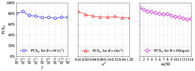
Figure 10: Optimal sample complexity of the EFG-$m$ procedure regarding $\gamma$, $\sigma^{2}$, and $m$

References

- Bechhofer et al. (1968) Bechhofer RE, Kiefer J, Sobel M (1968) Sequential identification and ranking procedures: with special reference to Koopman-Darmois populations (The University of Chicago Press).
- Bubeck et al. (2013) Bubeck S, Wang T, Viswanathan N (2013) Multiple identifications in multi-armed bandits. International Conference on Machine Learning, 258–265 (PMLR).
- Chang and Kuo (2018) Chang KH, Kuo PY (2018) An efficient simulation optimization method for the generalized redundancy allocation problem. European Journal of Operational Research 265(3):1094–1101.
- Chen et al. (2008) Chen CH, He D, Fu M, Lee LH (2008) Efficient simulation budget allocation for selecting an optimal subset. INFORMS Journal on Computing 20(4):579–595.
- Chen and Lee (2011) Chen CH, Lee LH (2011) Stochastic simulation optimization: an optimal computing budget allocation, volume 1 (World scientific).
- Eckman and Henderson (2021) Eckman DJ, Henderson SG (2021) Fixed-confidence, fixed-tolerance guarantees for ranking-and-selection procedures. ACM Transactions on Modeling and Computer Simulation (TOMACS) 31(2):1–33.
- Eckman et al. (2020) Eckman DJ, Plumlee M, Nelson BL (2020) Revisiting subset selection. 2020 Winter Simulation Conference (WSC), 2972–2983 (IEEE).
- Frazier et al. (2022) Frazier PI, Cashore JM, Duan N, Henderson SG, Janmohamed A, Liu B, Shmoys DB, Wan J, Zhang Y (2022) Modeling for COVID-19 college reopening decisions: Cornell, a case study. Proceedings of the National Academy of Sciences 119(2):e2112532119.
- Gao and Chen (2015) Gao S, Chen W (2015) Efficient subset selection for the expected opportunity cost. Automatica 59:19–26.
- Gao and Chen (2016) Gao S, Chen W (2016) A new budget allocation framework for selecting top simulated designs. IIE Transactions 48(9):855–863.
- Hong et al. (2021) Hong LJ, Fan W, Luo J (2021) Review on ranking and selection: A new perspective. Frontiers of Engineering Management 8(3):321–343.
- Hong et al. (2022) Hong LJ, Jiang G, Zhong Y (2022) Solving large-scale fixed-budget ranking and selection problems. INFORMS Journal on Computing 34(6):2930–2949.
- Jogdeo and Samuels (1968) Jogdeo K, Samuels SM (1968) Monotone convergence of binomial probabilities and a generalization of Ramanujan’s equation. The Annals of Mathematical Statistics 39(4):1191–1195.
- Kalyanakrishnan and Stone (2010) Kalyanakrishnan S, Stone P (2010) Efficient selection of multiple bandit arms: Theory and practice. ICML, volume 10, 511–518.
- Kalyanakrishnan et al. (2012) Kalyanakrishnan S, Tewari A, Auer P, Stone P (2012) PAC subset selection in stochastic multi-armed bandits. ICML, volume 12, 655–662.
- Kerr et al. (2021a) Kerr CC, Mistry D, Stuart RM, Rosenfeld K, Hart GR, Núñez RC, Cohen JA, Selvaraj P, Abeysuriya RG, Jastrzȩbski M, et al. (2021a) Controlling COVID-19 via test-trace-quarantine. Nature communications 12(1):2993.
- Kerr et al. (2021b) Kerr CC, Stuart RM, Mistry D, Abeysuriya RG, Rosenfeld K, Hart GR, Núñez RC, Cohen JA, Selvaraj P, Hagedorn B, et al. (2021b) Covasim: an agent-based model of COVID-19 dynamics and interventions. PLOS Computational Biology 17(7):e1009149.
- Kim and Nelson (2006) Kim SH, Nelson BL (2006) Selecting the best system. Handbooks in Operations Research and Management Science, volume 13, 501–534 (Elsevier).
- Koenig and Law (1985) Koenig LW, Law AM (1985) A procedure for selecting a subset of size m containing the l best of k independent normal populations, with applications to simulation. Communications in Statistics-Simulation and Computation 14(3):719–734.
- Li et al. (2024) Li Z, Fan W, Hong LJ (2024) The (surprising) sample optimality of greedy procedures for large-scale ranking and selection. Management Science Ahead of Print.
- Luce (1956) Luce RD (1956) Semiorders and a theory of utility discrimination. Econometrica 24(2):178–191.
- Luo et al. (2022) Luo X, Li L, Zhao L, Lin J (2022) Dynamic intra-cell repositioning in free-floating bike-sharing systems using approximate dynamic programming. Transportation Science 56(4):799–826.
- Monks and Currie (2018) Monks T, Currie CS (2018) Practical considerations in selecting the best set of simulated systems. 2018 Winter Simulation Conference (WSC), 2191–2200 (IEEE).
- Nelson et al. (2001) Nelson BL, Swann J, Goldsman D, Song W (2001) Simple procedures for selecting the best simulated system when the number of alternatives is large. Operations Research 49(6):950–963.
- Ni et al. (2017) Ni EC, Ciocan DF, Henderson SG, Hunter SR (2017) Efficient ranking and selection in parallel computing environments. Operations Research 65(3):821–836.
- Paleshi et al. (2017) Paleshi A, Bae KH, Evans G, Heragu S (2017) A simulation-based optimization approach for mitigation of pandemic influenza. IISE Transactions on Healthcare Systems Engineering 7(2):107–120.
- Pei et al. (2024) Pei L, Nelson BL, Hunter SR (2024) Parallel adaptive survivor selection. Operations Research 72(1):336–354.
- Peng et al. (2018) Peng Y, Chong EK, Chen CH, Fu MC (2018) Ranking and selection as stochastic control. IEEE Transactions on Automatic Control 63(8):2359–2373.
- Xiao et al. (2019) Xiao H, Chen H, Lee LH (2019) An efficient simulation procedure for ranking the top simulated designs in the presence of stochastic constraints. Automatica 103:106–115.
- Zhang et al. (2023) Zhang G, Peng Y, Zhang J, Zhou E (2023) Asymptotically optimal sampling policy for selecting top-m alternatives. INFORMS Journal on Computing 35(6):1261–1285.
- Zhang et al. (2012) Zhang S, Lee LH, Chew EP, Chen CH, Jen HY (2012) An improved simulation budget allocation procedure to efficiently select the optimal subset of many alternatives. 2012 IEEE International Conference on Automation Science and Engineering (CASE), 230–236 (IEEE).
- Zhang et al. (2015) Zhang S, Lee LH, Chew EP, Xu J, Chen CH (2015) A simulation budget allocation procedure for enhancing the efficiency of optimal subset selection. IEEE Transactions on Automatic Control 61(1):62–75.
- Zhao and Liu (2003) Zhao R, Liu B (2003) Stochastic programming models for general redundancy-optimization problems. IEEE Transactions on Reliability 52(2):181–191.
- Zhong and Hong (2022) Zhong Y, Hong LJ (2022) Knockout-tournament procedures for large-scale ranking and selection in parallel computing environments. Operations Research 70(1):432–453.

References

- Audibert et al. (2010) Audibert JY, Bubeck S, Munos R (2010) Best arm identication in multi-armed bandits. Proceedings of the 23rd Annual Conference on Learning Theory (COLT), 41-53.
- Bubeck et al. (2013) Bubeck S, Wang T, Viswanathan N (2013) Multiple identifications in multi-armed bandits. International Conference on Machine Learning, 258–265 (PMLR).
- Chen et al. (2008) Chen CH, He D, Fu M, Lee LH (2008) Efficient simulation budget allocation for selecting an optimal subset. INFORMS Journal on Computing 20(4):579–595.
- Gabillon et al. (2012) Gabillon V, Ghavamzadeh M, Lazaric A (2012) Best arm identification: A unified approach to fixed budget and fixed confidence. Advances in Neural Information Processing Systems, 25.
- Li et al. (2024) Li Z, Fan W, Hong LJ (2024) The (surprising) sample optimality of greedy procedures for large-scale ranking and selection. Management Science Ahead of Print.
- Wu and Zhou (2018) Wu D, Zhou E (2018) Analyzing and provably improving fixed budget ranking and selection algorithms. arXiv preprint arXiv:1811.12183.
- Zhang et al. (2023) Zhang G, Peng Y, Zhang J, Zhou E (2023) Asymptotically optimal sampling policy for selecting top-m alternatives. INFORMS Journal on Computing 35(6):1261–1285.
- Zhong and Hong (2022) Zhong Y, Hong LJ (2022) Knockout-tournament procedures for large-scale ranking and selection in parallel computing environments. Operations Research 70(1):432–453.