Fine-gained air quality inference based on low-quality sensing data using self-supervised learning

Abstract.

Fine-grained air quality (AQ) mapping is made possible by the proliferation of cheap AQ micro-stations (MSs). However, their measurements are often inaccurate and sensitive to local disturbances, in contrast to standardized stations (SSs) that provide accurate readings but fall short in number. To simultaneously address the issues of low data quality (MSs) and high label sparsity (SSs), a multi-task spatio-temporal network (MTSTN) is proposed, which employs self-supervised learning to utilize massive unlabeled data, aided by seasonal and trend decomposition of MS data offering reliable information as features. The MTSTN is applied to infer NO₂, O₃ and PM_2.5 concentrations in a 250 km² area in Chengdu, China, at a resolution of 500m$\times$500m$\times$1hr. Data from 55 SSs and 323 MSs were used, along with meteorological, traffic, geographic and timestamp data as features. The MTSTN excels in accuracy compared to several benchmarks, and its performance is greatly enhanced by utilizing low-quality MS data. A series of ablation and pressure tests demonstrate the results’ robustness and interpretability, showcasing the MTSTN’s practical value for accurate and affordable AQ inference.

1. Introduction

As the serious health hazards of air pollution are gradually revealed (MXCRFAASMP2021, ; AD2014, ), public demand for air quality improvement has become increasingly urgent. Fine-grained air quality information, crucial for air quality management, has received worldwide attention across academia and industry. However, obtaining this information through direct measurement is practically challenging. While standardized stations provide accurate and reliable measurements, their deployment is spatially sparse due to the high costs of construction and maintenance ($100,000$\sim$300,000 for construction and over $100,000 per year for maintenance) (AMGB2017, ). In contrast, cheap micro-stations can be ubiquitously deployed, offering a possible solution, but their readings are often inaccurate and sensitive to local disturbances. Consequently, fusing these two types of data for accurate and affordable air quality inference has significant scientific and practical values, which is addressed in this work.

Air quality inference is a challenging problem due to the complex and dynamic spatio-temporal dependencies of pollutant concentrations on various factors. Additionally, it is a few-labeled problem owing to the limited number of standardized stations. Over the past decade, spatio-temporal neural networks have gained popularity in this area for their remarkable competence in learning spatio-temporal dependencies. Among them, the most prevalent are the various kinds of supervised learning models (HJYZLYR2023, ; CWYYL2018, ; HJYHYZR2023, ). However, these models fail to address the sparsity of labels, underutilizing unlabeled data that constitute a majority portion. To overcome this issue, many researchers have pivoted towards semi-supervised learning models (CLYYMCG2016, ; ZYFH2013, ), which leverage both labeled and unlabeled data during the training process. Self-supervised learning models also demonstrate considerable competence in addressing few-labeled challenge (RDAFMSFPMB2018, ; JWTHYSZJ2020, ), but exhibit a gap in exploring air quality inference so far. Consequently, self-supervised learning models are novel and promising tools for air quality inference.

In this work, a self-supervised learning framework, called Multi-Task Spatio-Temporal Network (MTSTN), is proposed for fine-grained air quality inference over the graph structure. The MTSTN involves a self-supervised task and a supervised task; the former acts as a pretext task, learning a valuable representation from unlabeled data, while the latter serves as the downstream task, executing the core inference. The self-supervised learning is designed as a regression inference task, utilizing the spatial interpolation results based on high-quality data from standardized stations as its labels. On the use of low-quality data, we employ Seasonal and Trend Decomposition using Loess (STL) (CRWJI1990, ) to extract relatively stable and reliable information from micro-station data, which is then used as features for self-supervised learning. Among the decomposition results, the trend exhibits high importance to the inference performance, showcasing the value of low-quality pervasive sensing data for accurate AQ inference. The main contributions of this paper are summarized as follows:

• This work explores the hidden values of low-quality data provided by cheap and pervasive AQ sensors, simultaneously addressing the issues of low data quality (offered by micro-stations) and high label sparsity (offered by standardized stations), which has significant practical values for accurate and affordable air quality inference.

• To achieve the above goal, we propose a novel Multi-Task Spatio-Temporal Network (MTSTN), which employs self-supervised learning to utilize massive unlabeled data, aided by seasonal and trend decomposition of micro-station data offering reliable spatio-temporal information as features. Compared to state-of-the-art baselines, this method results in higher inference accuracy.

• A method for the selection of both continuous and categorical features and importance assessment is proposed, by incorporating their gradients as regularization terms in the loss function, which further improves the model’s accuracy and interpretability. Notably, in a real-world case study, trend from micro-station data decomposition turns out to be the most significant feature, showcasing the practical value of low-quality yet pervasive sensing data for accurate air quality inference.

2. Results

2.1. Problem Formalization

Given the air quality graph $\mathcal{G}$, which represents the spatial position information of the study area, and two types of features: Grid features $\chi$ and graph topologies $\bm{A}$, as defined in Appendix A, the objective of air quality inference is to learn a function $\mathcal{F}$ that can accurately infer pollutant concentration $Y_{t}$. In summary, the air quality inference problem can be formulated as follows:

(1) $$Y_{t}=\mathcal{F}\left[\chi_{\left(t-\tau+1\right)},...,\chi_{t};\bm{A};\mathcal{G}\right]$$

where $t$ and $\tau$ are timestamp and time window respectively.

2.2. Dataset and features

This is based on a real-world dataset in the central region (250 km²) of Chengdu, China, between 1st Mar. and 1st Apr. 2022. Space is meshed into 999 grids of size 500m$\times$500m (as depicted in Fig. 1), and time is discretized into 1-hr intervals. Additionally, 5 types of datasets are collected: hourly pollutant (NO₂, O₃, PM_2.5) concentrations from standardized and micro-stations, hourly meteorological data, traffic data (hourly road congestion index and truck GPS trajectories), geographic data from OpenStreetMap, and timestamp data. Based on these datasets, 5 types of features are designed, with a total number of 42. Detailed descriptions and visualizations of other features are provided in Appendix A.

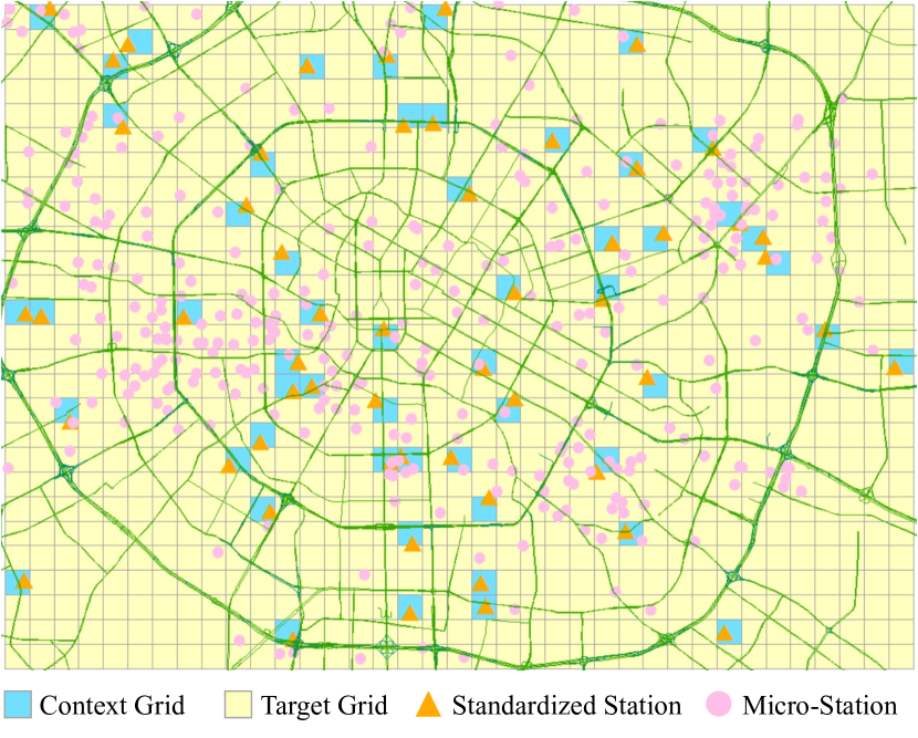
Figure 1. Distribution of 378 air quality monitoring stations (55 standardized stations and 323 micro-stations) across the central region of Chengdu, China. The context (labeled) grids have standardized stations, while the target (unlabeled) grids do not.

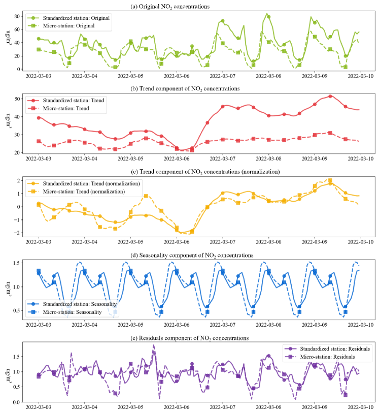
Figure 2. NO₂ concentrations and their decomposition results during Mar. 3 - 10, 2022

As a hallmark of this work, the decomposition of micro-station data (NO₂ concentration) is illustrated. Fig. 2 (a) shows the NO₂ concentrations from both standardized and micro-stations within the same grid. It is apparent that the two NO₂ concentrations differ numerically, but exhibit a non-linear correlation. Therefore, before utilizing the pollutant concentrations collected by micro-stations, it is crucial to extract a valuable component from them. To achieve this, Seasonal and Trend Decomposition using Loess (STL) (CRWJI1990, ) is applied to mine pollutant concentrations, decomposing them into trend, seasonality and residuals, as shown in Fig. 2 (b), (d) and (e). The decomposition results reveal similarity in trend and seasonality from the two data sources. Seasonality indicates that NO₂ concentrations increase nocturnally, likely due to the atmospheric titration effect, where lower temperatures and reduced solar radiation at night enhance the reaction between NO and O₃, leading to increased NO₂ formation. This finding supports the reliability of the decomposition results. To avoid feature redundancy, seasonality is not employed as a feature because other features (e.g. timestamps) can better indicate the periodicity of pollutant concentrations. Fig. 2 (b) shows highly correlated trends, but with distinct numerical values due to the sensors’ characteristics. To overcome this issues, we normalize their trend, as demonstrated in Fig. 2 (c). After normalization, the numerical values of the two trends demonstrate a high degree of consistency. Consequently, normalized trend (abbreviated as trend) is employed as a feature for air quality inference.

As demonstrated in Fig. 3, the study area is segmented into four parts: interpolation grids, training grids, validation grids and test grids, which are designed to generate labels for self-supervised tasks, train the model, select hyperparameters and evaluate model performance respectively. Due to the few-labeled issue, only 20% of the context grids are set as interpolation grids and 10% are set as test grids. For the remaining 70% of the context grids, a 3-fold cross-validation is implemented to reduce parameter selection randomness and improve model confidence. The average evaluation metrics on the test grids are employed to quantify model performance, including mean absolute error (MAE), root mean square errror (RMSE) and r-square (R²), which are commonly used in regression problems. To validate MTSTN’s generalizability in pollutant concentration inference, experiments are conducted on three pollutants: NO₂, O₃ and PM_2.5.

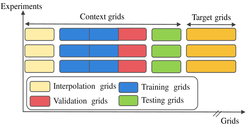
Figure 3. Evaluation strategy and dataset segmentation.

2.3. Loss function

To implement both continuous and categorical feature selection, two gradient-based regularization terms are incorporated into the loss function, formulated as follows:

(2) $$\theta^{*},\varTheta^{*},\varTheta_{\text{ss}}^{*} =\underset{\theta,\varTheta,\varTheta_{\text{ss}}}{\text{argmin}}\left(1-\beta-\gamma\right)\left(\alpha_{\text{sup}}\mathcal{L}_{\left(\theta,\varTheta\right)}+\alpha_{\text{ss}}\mathcal{L}_{\left(\theta,\varTheta_{\text{ss}}\right)}\right)$$

$$+\beta\sum_{i=1}^{U}{\left\|\frac{\partial\mathcal{L}\left(X_{\text{num}},\hat{Y}\right)}{\partial X_{\text{num}}^{i}}\right\|_{2}+}\gamma\sum_{j=1}^{V}{\sum_{q=1}^{Q_{j}}{\left\|\frac{\partial\mathcal{L}\left(X_{\text{cat}},\hat{Y}\right)}{\partial X_{\text{cat}}^{q}}\right\|_{2}}}$$

$$\mathcal{L} =\frac{1}{\left|Y_{\text{train}}\right|}\sum_{y_{n}\in Y_{\text{train}}}{\left|y_{n}-\hat{y}_{n}\right|}$$

where $\theta^{*},\varTheta^{*},\varTheta_{\text{ss}}^{*}$ are learnable parameters. $\alpha_{\text{sup}},\alpha_{\text{ss}}\in\mathbb{R}_{>0}$ serve as the loss weights for the supervised and self-supervised task respectively, which affect the role of each task on model’s training process. $\beta$ and $\gamma$ are regularization coefficients for feature selection. $U$ and $V$ are the numbers of continuous and categorical features respectively. $Q_{j}$ is the embedding dimension corresponding to the $j^{th}$ categorical feature. $\mathcal{L}$ is the function quantifying the discrepancy between ground truth $y_{n}$ and inference value $\hat{y}_{n}$ within the training dataset $Y{\text{train}}$.

2.4. Model configurations

All experiments are implemented with PyTorch 2.1 and trained on an NVIDIA GeForce RTX 4090 GPU. The loss function is minimized by Adam optimizer. To prevent overfitting and optimize training efficiency, the training process is allowed to be early stopped according to the performance on validation grids. More details about experiment settings and hyperparameters can be found in Appendix B.1.

2.5. Baselines

Several baselines with different architectures are selected to compare their performances with MTSTN, including K-Nearest Neighbors (KNN), Inverse Distance Weighting (IDW), Land Use Regression (LUR), Random Forest (RF), Extreme Gradient Boosting (XGBoost), Spatio-Temporal Graph Convolutional Networks (STGCN), Multi-View Spatial-Temporal Graph Convolutional Networks (MSTGCN), Attention-based Spatial-Temporal Graph Neural Networks (ASTGNN) and Propagation Delay-Aware Dynamic Long-Range Transformer (PDFormer). More details about baselines can be found in Appendix B.2. For a fair comparison, different hyperparameters are tuned for each baseline to find their optimal settings.

2.6. Overall performance

Table 1 reports the overall performance of MTSTN and other baselines on the dataset. The MTSTN significantly outperforms all baselines across nearly every metric, demonstrating its superiority. Moreover, among the three pollutants, PM_2.5 has the lowest inference accuracy, primarily attributed to its high variability. This variability is mainly caused by the complexity of its sources and composition, as well as its extremely fine particle size, which complicates monitoring efforts. In addition, compared to certain deep learning models (STGCN, MSTGCN, ASTGNN, and PDFormer), traditional decision tree models such as RF and XGBoost demonstrate superior performance, highlighting that deep learning models do not consistently outperform decision tree models (GYIVA2021, ).

Table 1. Performance comparison between MTSTN and the baselines. The bold/underlined fonts mean the best/the second best results. Benchmarked performance denotes the degree of change in MTSTN relative to the best baseline, where $\uparrow$ indicates performance improvement, and $\downarrow$ signifies performance deterioration.

Model	NO2			O3			PM2.5
	MAE	RMSE	R2	MAE	RMSE	R2	MAE	RMSE	R2
KNN (Hu et al. (CT1968, ), 1968)	6.806	9.400	0.668	4.303	6.917	0.856	11.137	15.082	0.755
IDW (Bartier et al. (BPC1996, ), 1996)	6.741	9.401	0.668	4.273	7.347	0.838	11.357	15.912	0.725
LUR (Briggs et al. (BDSPPSEKHK1997, ), 1997)	7.193	9.906	0.632	6.526	10.105	0.696	12.369	15.555	0.739
RF (Breiman et al. (BL2001, ), 2001)	$\underline{4.206}$	$\underline{5.933}$	$\underline{0.868}$	2.881	$\underline{4.691}$	$\underline{0.934}$	8.153	11.051	0.868
XGBoost (Chen et al. (CTTMVYHKRIT2015, ), 2015)	4.428	6.261	0.853	3.160	5.042	0.924	$\underline{8.070}$	10.663	$\underline{0.877}$
STGCN (Yu et al. (YBHZ2017, ), 2017)	5.594	7.466	0.796	3.901	5.993	0.891	8.378	11.376	0.855
MSTGCN (Jia et al. (JZYJXYRYH2021, ), 2021)	4.857	6.462	0.823	3.957	6.097	0.904	10.489	13.744	0.807
ASTGNN (Guo et al. (GSYHX2021, ), 2021)	5.860	7.634	0.789	5.594	9.644	0.723	15.191	11.344	0.763
PDFormer (Jiang et al. (JJCWJ2023, ), 2023)	5.326	7.289	0.809	5.231	7.755	0.839	10.281	13.565	0.810
MTSTN (Proposed method, 2024)	3.758	5.242	0.910	$\underline{3.042}$	4.574	0.947	7.767	$\underline{10.666}$	0.883
Benchmarked performance	$\uparrow$ 10.65%	$\uparrow$ 11.65%	$\uparrow$ 4.84%	$\downarrow$ 5.59%	$\uparrow$ 2.49%	$\uparrow$ 1.39%	$\uparrow$ 3.75%	$\downarrow$ 0.03%	$\uparrow$ 0.68%

2.7. Feature importance

Feature selection and importance assessment are crucial for improving the model accuracy and interpretability. Feature importance is calculated based on the gradients, which guide the weights update in neural networks. A larger gradient value indicates greater importance of the feature. Since categorical features are embedded before being input into the feature encoder module, distinct methods are implemented to determine the importance of continuous and categorical features, which are formulated as follows:

(3) $$p_{\text{num}}^{i} =\left\|\frac{\partial\mathcal{L}\left(X_{\text{num}},Y\right)}{\partial X_{\text{num}}^{i}}\right\|$$

$$p_{\text{cat}}^{j} =\frac{\sum_{q=1}^{Q_{j}}{\left\|\frac{\partial\mathcal{L}\left(X_{\text{cat}},Y\right)}{\partial X_{\text{cat}}^{q}}\right\|}}{Q_{j}}$$

where $p_{\text{num}}^{i}$ and $p_{\text{cat}}^{j}$ denote the importance of the $i^{\text{th}}$ numerical feature and the $j^{\text{th}}$ categorical feature respectively.

Fig. 4 reports the rankings of top 20 features. The following are observed: a) The feature trend takes the top position for all three pollutants, highlighting the significance of using low-quality data from micro-stations. b) For a given pollutant, other pollutants’ concentrations are significant features. For example, NO₂ and O₃ concentrations are important features to each other, confirming their chemical interaction (the titration effect); in addition, NO₂ concentration ranks 2${}^{\text{nd}}$ for PM_2.5 inference, as the former may contributes to the nocturnal formation of nitrate particles, which are a significant component of PM_2.5 (FZLHZXDCSF2021, ; YTNXWGMZHL2023, ). c) Meteorological features take up over half of the top 10 rankings, suggesting their critical roles in pollutant formation and dissipation. d) Periodicity in the pollutant concentrations is represented by the feature hour of day, which is ranked 10 (NO₂), 11 (O₃), and 16 (PM_2.5). Indeed, this is confirmed by Fig. S4. in Appendix A.5. e) Grid congestion index, ranking 1${}^{\text{st}}$ among all features related to human activities, implies that traffic congestion levels have a significant impact on these pollutant concentrations, highlighting the critical role of congestion mitigation in combating air pollution.

2.8. Ablation study

To investigated the effectiveness of each core module in MTSTN, a set of ablation experiments are conducted. The experimental results are reported in Table 2

(1) Effects of self-supervised task: To evaluate the effectiveness of proposed self-supervised task, it is compared with three variants: a) w/o SST: removing self-supervised task; b) r/p KSST: replacing IDW with KNN. c) r/p GSST: replacing the self-supervised task with the graph completion task. Removing the self-supervised task leads to a degradation in MAE, RMSE and R², revealing the powerful learning capability of the self-supervised task. Additionally, r/p GSST exhibits inferior performance compared to MTSTN and w/o KSST, because the self-supervised task of r/p GSST is graph completion, while those of the latter two are spatio-temporal regression inference tasks which are analogous to the supervised task.

(2) Effects of positional embedding module: The positional embedding module is removed (w/o PE) to examine its efficacy. Results indicate that the MTSTN’s performance declines after the removal, highlighting the significance of grids’ relative positional correlations for air quality inference.

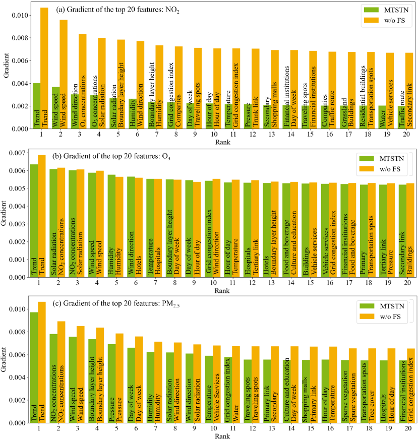
Figure 4. Key feature ranking

(3) Effects of feature selection: A model is constructed without the proposed feature selection method (w/o FS), whose deteriorated performance underscores the crucial role of feature selection in air quality inference. Fig. 4 illustrates the key features of both w/o FS and MTSTN. Using NO₂ as an example, temperature and pressure, both strongly correlated with NO₂ concentrations (VACMMAB2002, ; GDSGAD2021, ), are identified as key features in MTSTN but not in w/o FS. This shows better adherence to the natural laws of air pollution by the proposed feature selection method.

(4) Effects of adjacency matrix: In this work, two adjacency matrices: OD adjacency matrix ($A^{\text{OD}}$) and semantic adjacency matrix ($A^{\text{SE}}$), are employed as features. Further details about these matrices are available in Appendix A.3 and Appendix A.4. Two removal experiments are conducted for each matrix, named w/o OD and w/o SE. Experimental results demonstrate that the removal of either $A^{\text{OD}}$ or $A^{\text{SE}}$ degrades the performance across all evaluation metrics, underscoring their essential role in air quality inference. Compared to $A^{\text{OD}}$, the removal of $A^{\text{SE}}$ leads to a more pronounced performance degradation, suggesting that $A^{\text{SE}}$ has a more substantial impact on air quality inference.

Table 2. Experimental results of ablation studies. The bold/underlined font mean the best/the second best result.

Model	NO2			O3			PM2.5
	MAE	RMSE	R2	MAE	RMSE	R2	MAE	RMSE	R2
MTSTN	3.758	5.242	0.910	3.042	4.574	0.947	7.767	10.666	0.883
w/o SST	4.221	5.818	0.886	3.254	5.032	0.936	11.008	14.611	0.774
r/p KSST	4.031	5.701	$\underline{0.892}$	3.554	5.735	0.916	10.221	13.353	0.813
r/p GSST	4.233	5.760	0.890	3.531	5.766	0.915	10.618	14.045	0.797
w/o PE	$\underline{3.956}$	$\underline{5.501}$	0.886	3.405	6.355	0.862	8.259	11.198	0.860
w/o FS	4.362	5.994	0.881	3.173	$\underline{4.842}$	$\underline{0.941}$	$\underline{8.004}$	$\underline{10.975}$	$\underline{0.876}$
w/o OD	4.212	5.859	0.884	$\underline{3.140}$	5.121	0.925	8.194	11.510	0.855
w/o SE	4.305	5.941	0.861	3.158	4.974	0.919	8.915	12.048	0.841

2.9. Missing ratio study

In reality, air quality monitoring stations often encounter signal loss due to maintenance or other unpredictable factors, making it essential to evaluate MTSTN’s performance with missing data. Consequently, the data is randomly corrupted according to a predetermined missing ratio, and then restored using linear interpolation. For data points still missing after interpolation, values from the next timestamp within the same grid are used to fill them. Fig. 5 reports the MAE and RMSE of MTSTN across missing ratios from 0.2 to 0.7, revealing that MTSTN’s performances decline for all three pollutants due to errors caused by filling missing values, with a generally progressive decrease as the missing ratio increased. However, the degree of this decrease is minimal, demonstrating MTSTN’s robustness. Notably, in real-world scenarios, the missing data ratio is typically low, so performance degradation remains within an acceptable range.

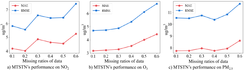
Figure 5. Data missing ratio study.

2.10. A Case Study on NO₂

Temporal analysis: Fig. 6 provides evidence that MTSTN achieves superior inference accuracy compared to the second best baseline (RF) for the majority of the observation period. In particular, during the periods highlighted in the red box, i.e., the time when the NO₂ concentrations around the peak, inference results of MTSTN are consistently closer to the ground truth than those of RF. This superior performance can be attributed to that MTSTN uses spatial interpolation results as labels for the self-supervised task, which provide a reference value for the NO₂ concentrations. Additionally, both MTSTN and RF exhibit trends that closely align with the ground truth, especially when the trend is notable and steady, as indicated in the yellow box. This alignment may be due to the incorporation of trend data.

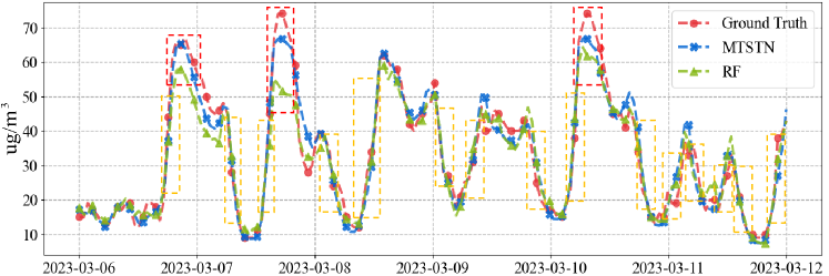
Figure 6. NO₂ concentration inference results on Chengdu’s dataset during the Mar. 6 - 12, 2022

Spatial analysis: Fig. 7 (a) illustrates the spatial distribution of daily mean NO₂ concentrations, highlighting that the central region and the areas west of the center consistently exhibit higher NO₂ concentrations. Fig. 7 (b) and Fig. 6 (c) demonstrate the spatial distribution of traffic spots and cropland respectively. Traffic spots presents a similar spatial distribution to NO₂ concentrations, suggesting that traffic is a significant contributor to NO₂ emissions. While cropland shows a spatial distribution diametrically opposed to NO₂ concentrations. This contrast may be partly due to the soil in croplands effectively adsorbing NO₂ and partly because croplands are typically located in suburban areas where NO₂ emissions are generally lower.

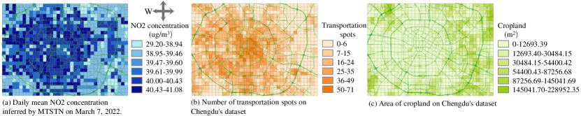
Figure 7. Spatial distribution of NO₂ concentration inference results, transportation spots and cropland.

3. Discussion

This paper proposes the Multi-Task Spatio-Temporal Network (MTSTN) for real-time and fine-grained air quality inference, which decouples the task into a supervised task and a self-supervised task. Notably, the self-supervised task can learn a valuable representation from unlabeled data, thus avoiding the data waste. For the readings collected by micro-stations, which are inaccurate and sensitive to local disturbances, Seasonal and Trend Decomposition using Loess (STL) is employed to extract their trend component, which is then utilized as a feature for inference. Furthermore, a gradient-based method for both continuous and categorical feature selection and importance assessment is proposed, effectively addressing the challenge of categorical feature selection and importance assessment. Experimental results demonstrate that MTSTN achieves significant performance improvement compared to other competitive baselines on Chengdu’s dataset. The feature importance ranking demonstrates that trend is the most important feature, highlighting the practical value of low-data-quality pervasive sensors for high-accuracy air quality inference.

4. Methods

4.1. Learning framework

Inspired by You et al. (YCTZY2020, ), a self-supervised learning framework called MTSTN is proposed, with the overall framework shown in Fig. 8. MTSTN comprises four key modules: positional embedding module, spatial interpolation module, feature encoder module, and feature decoder module. Inference begins by processing the categorical features within the input $[\chi_{\left(t-\tau+1\right)},...,\chi_{t};A^{\text{OD}};A^{\text{SE}};\mathcal{G}]$ using categorical feature embedding. To capture relative position correlations, the embedding $[\chi^{\prime}_{\left(t-\tau+1\right)},...,\chi^{\prime}_{t};A^{\text{OD}};A^{\text{SE}};\mathcal{G}]$ is processed through positional embedding module, producing a new embedding $[\chi^{\prime}_{\left(t-\tau+1\right)},...,\chi^{\prime}_{t};A^{\text{OD}};A^{\text{SE}};PE]$. This embedding is then used in two parallel pathways: one utilized by spatial interpolation module to generate labels $\hat{Y}_{t}^{ss}$ for the self-supervised learning, and the other employed by feature encoder module to learn a representation $H_{t}^{3}$. This representation is subsequently processed by feature decoder module, computing inference results for both self-supervised task and supervised task.

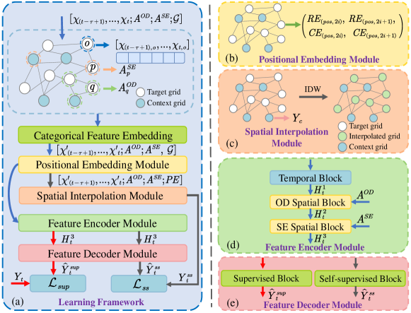
Figure 8. The overall framework. Red arrows show the information flow pertinent to the supervised task, gray arrows indicate the information flow for the self-supervised task and blue arrows represent the shared components between both of them. (a) Learning framework of MTSTN. (b) Positional embedding module. (c) Spatial interpolation module. (d) Feature encoder module. (e) Feature decoder module.

4.2. Positional embedding module

Considering the robust correlation between pollutant concentrations and spatial position, a positional embedding module is incorporated to enhance the spatial awareness of MTSTN, as shown in Fig. 8 (b). Inspired by masked autoencoder (HKXSY2022, ) and transformer (VANNJLA2017, ), sine and cosine functions are employed to construct positional embedding module. Specifically, positional embedding module consists of two distinct embeddings: row embedding (RE) and column embedding (CE), which can be represented as follows:

(4) $$RE_{\left(\text{pos}_{r},2i\right)} =\sin\left(pos_{r}/10000^{4i/d_{p}}\right)$$

$$RE_{\left(\text{pos}_{r},2i+1\right)} =\cos\left(pos_{r}/10000^{4i/d_{p}}\right)$$

$$CE_{\left(\text{pos}_{c},2i\right)} =\sin\left(pos_{c}/10000^{4i/d_{p}}\right)$$

$$CE_{\left(\text{pos}_{c},2i+1\right)} =\cos\left(pos_{c}/10000^{4i/d_{p}}\right)$$

where $\text{pos}_{r}$ and $\text{pos}_{c}$ denote the row position and column position respectively, and $d_{p}$ signifies the dimension.

4.3. Spatial interpolation module

To learn a valuable representation, the self-supervised task should be thoughtfully designed (SXWHQ2021, ). Considering a self-supervised task analogous to the supervised task may improve the accuracy of air quality inference, this work structures the self-supervised task as a regression inference task, mirroring to the supervised task. As shown in Fig. 8 (c), Inverse Distance Weighting (IDW) (Eqn. 5) is used to spatially interpolate the pollutant concentrations, and the interpolation results then serve as the labels for the self-supervised task. IDW is renowned as a deterministic model for spatial interpolation, praised for its computational efficiency, ease of calculation, and clear interpretability (LGD2008, ).

(5) $$X_{g}= \frac{1/d_{gc}^{p}}{\sum\nolimits_{1}^{C}{1/d_{gc}^{p}}}\times X_{c}$$

$$d_{gc}= 2r\arcsin\sqrt{\sin^{2}\left(\frac{\phi_{g}-\phi_{c}}{2}\right)+\cos(\phi_{c})\cos(\phi_{g})\sin^{2}\left(\frac{\lambda_{g}-\lambda_{c}}{2}\right)}$$

where $X_{g}$ denotes the interpolation results for the target grid $r_{g}$. $d_{gc}^{k}$ represents the great-circle distance between the target grid $r_{g}$ and the context grid $r_{c}$, with $p$ as a constant. $r$ is the radius of the earth, i.e., $6371$ km, and both the longitude ($\phi_{n}$) and latitude ($\lambda_{n}$) of $r_{n}$ are expressed in radians.

4.4. Feature encoder module

To capture complex and dynamic spatio-temporal dependencies of pollutant concentrations, the feature encoder module is designed as a spatio-temporal (ST) encoder module. As depicted in Fig. 8(d), this module is structured with a temporal block followed by two spatial blocks. Notably, within the feature encoder module, the supervised task and the self-supervised task share parameters, facilitating information sharing across tasks and consequently improving the accuracy of air quality inference.

Temporal Block. To capture the sequential patterns of pollutant concentrations across different timestamps, temporal block (TB) employs the bidirectional long-short term memory (Bi-LSTM) with the gated mechanism (SMPK1997, ), which preserves both past and future information. Specifically, TB takes $(\chi^{\prime}_{(t-\tau+1)},...,\chi^{\prime}_{t};PE)$ as input, and outputs a time-aware representation:

(6) $$H_{t}^{1}=TB\left(\chi^{\prime}_{\left(t-\tau+1\right)},...,\chi^{\prime}_{t};PE\right)$$

where $H_{t}^{1}=\{\vec{h}_{t,1}^{1},...,\vec{h}_{t,N}^{1}\}\in\mathbb{R}^{N\times d_{t}}$ denotes the time-aware representation at timestamp $t$, and $d_{t}$ represents the embedding dimension.

Each LSTM, whether operating in the forward or backward direction, is equipped with three gates: forget (Eqn.7), input (Eqn.8), and output (Eqn.9) gates. These gates regulate the information flow, allowing LSTM to selectively preserve, refresh or eliminate information, thereby optimizing the feature learning process for complex temporal patterns.

(7) $$f_{t}=\sigma\left(W_{f}\left[h_{t-1},\bm{\chi}\prime_{\bm{t}}\right]+b_{f}\right)$$

where $f_{t}$ is the forget gate, responsible for deciding whether to retain or discard the existing memory. $h_{t-1}$ denotes the hidden vector at timestamp $t-1$ and $\bm{\chi}_{t}^{\prime}=(\chi^{\prime}_{t};PE)$ signifies the input at timestamp $t$. $\sigma$ is the sigmoid function, while $W_{f}$ and $b_{f}$ are all learnable parameters.

(8) $$i_{t} =\sigma\left(W_{i}\left[h_{t-1},\bm{\chi}_{t}^{\prime}\right]+b_{i}\right)$$

$$\tilde{C}_{t} =\tanh\left(W_{c}\left[h_{t-1},\bm{\chi}_{t}^{\prime}\right]+b_{c}\right)$$

$$C_{t} =f_{t}C_{t-1}+i_{t}\tilde{C}_{t}$$

where $i_{t}$ is the input gate, tasked with deciding whether to introduce new memory and what type of memory to introduce. $\tilde{C}_{t}$ indicates candidate memory, $C_{t}$ represents cell state.

(9) $$o_{t} =\sigma\left(W_{o}\left[h_{t-1},\bm{\chi}_{t}^{\prime}\right]+b_{o}\right)$$

$$h_{t} =o_{t}\tanh\left(C_{t}\right)$$

where $o_{t}$ is the output gate, responsible for determining which part of memory contributes to the output. $h_{t}$ is the final output

Spatial Blocks. To capture complex spatial dependencies, two distinct spatial blocks are designed: origin-destination spatial block (ODSB), utilizing

$$A^{\text{OD}}$$

, and semantic spatial block (SESB), employing $A^{\text{SE}}$. This two blocks are formulated as follows:

(10) $$H_{t}^{2} =\text{ODSB}\left(H_{t}^{1},A^{\text{OD}}\right)$$

$$H_{t}^{3} =\text{SESB}\left(H_{t}^{2},A^{\text{SE}}\right)$$

Both two spatial blocks employ graph attention layers (VPGAAPY2017, ), which assign different weights to neighboring nodes. The core of graph attention layers is the attention coefficient $\alpha_{ij}$, calculated as follows:

(11) $$\alpha_{ij} =\frac{\exp\left(\text{Leaky}\mathrm{Re}LU\left(e_{ij}\right)\right)}{\sum_{k\in\mathcal{N}\left(r_{i}\right)}{\exp\left(\text{Leaky}\mathrm{Re}LU\left(e_{ij}\right)\right)}}$$

$$e_{ij} =a\left(\left[WH_{t,i}\left\|WH_{t,j}\right.\right]\right),r_{j}\in\mathcal{N}\left(r_{i}\right)$$

where $e_{ij}$ quantifies the importance of grid $r_{i}$ to its neighbor $r_{j}$. $\mathcal{N}\left(r_{i}\right)$ is the set of neighboring grids for grid $r_{i}$. $a$ denotes the shared attention mechanism that maps high-dimensional features to a scalar value. $W$ is a learnable parameter.

Subsequently, utilizing $\alpha_{ij}$, the output $H_{t}(K)$ of the graph attention layers is as follows:

(12) $$H_{t}\left(K\right)\,\,=\,\,\underset{k=1}{\overset{K}{||}}\sigma\left(\sum_{r_{j}\in\mathcal{N}_{r_{i}}}{\alpha_{ij}^{k}W^{k}H_{t,j}}\right)$$

where $K$ indicates the number of attention heads.

4.5. Feature decoder module

Within the feature decoder module, different blocks are designed for distinct subtasks, as shown in Fig 8 (e). Supervised task adopts a spatial block (SUPB) with graph attention layers, while self-supervised task employs a simpler block (SSB) with fully connected layers, which can be described as follows:

(13) $$\hat{Y}_{t}^{\text{sup}} =\text{SUPB}\left(H_{t}^{3}\right)(\text{supervised task})$$

$$\hat{Y}_{t}^{\text{ss}} =\text{SSB}\left(H_{t}^{3}\right)(\text{self-supervised task})$$

where $\hat{Y}_{t}^{\text{sup}}\in\mathbb{R}^{N\times d_{\text{sup}}}$ and $\hat{Y}{t}^{ss}\in\mathbb{R}^{N\times d_{\text{ss}}}$ represent the inference results for the supervised task and self-supervised task, with $d_{\text{sup}}$ and $d_{\text{ss}}$ representing their corresponding output dimensions.

1

5. Acknowledgements

This work is supported by the National Natural Science Foundation of China through grant no. 72071163.

6. Author contributions

M.X. and K.H conceived and led the research project. K.H. provides advice on feature and framework design. M.X designed and implemented the framework, producing experimental results. M.X. and K.H. wrote the paper. W.H. and W.J. contributed with ideas to improve the work. All authors reviewed the manuscript.

Appendix Appendix A Dataset and features

Appendix A.1. Air quality data

Due to the high-quality of standardized stations, target pollutant concentrations from them are employed as labels for the supervised task. Additionally, chemical reactions between pollutants create correlations in their concentrations, as illustrated in Fig. Appendix 1. For example, NO₂ and O₃ transform into each other under certain meteorological conditions, and NO₂ can react chemically with other pollutants to produce PM_2.5 (HSHYAXFX2011, ; CLM2001, ; CP1979, ). Consequently, the most relevant pollutant ($Y^{\text{REP}}$) is utilized as feature for air quality inference. However, the spatial sparsity of the standardized stations results in a large number of missing values for raw $Y^{\text{REP}}$. Therefore, IDW is employed to spatially interpolate these values, and the interpolation results are used as the final $Y^{\text{REP}}$.

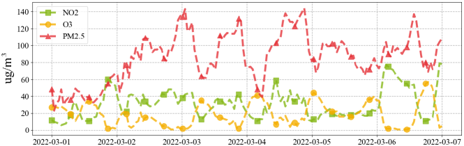
Figure Appendix 1. NO₂, O₃ and PM_2.5 concentrations during Mar. 1 - 7, 2022

Appendix A.2. Meteorological data

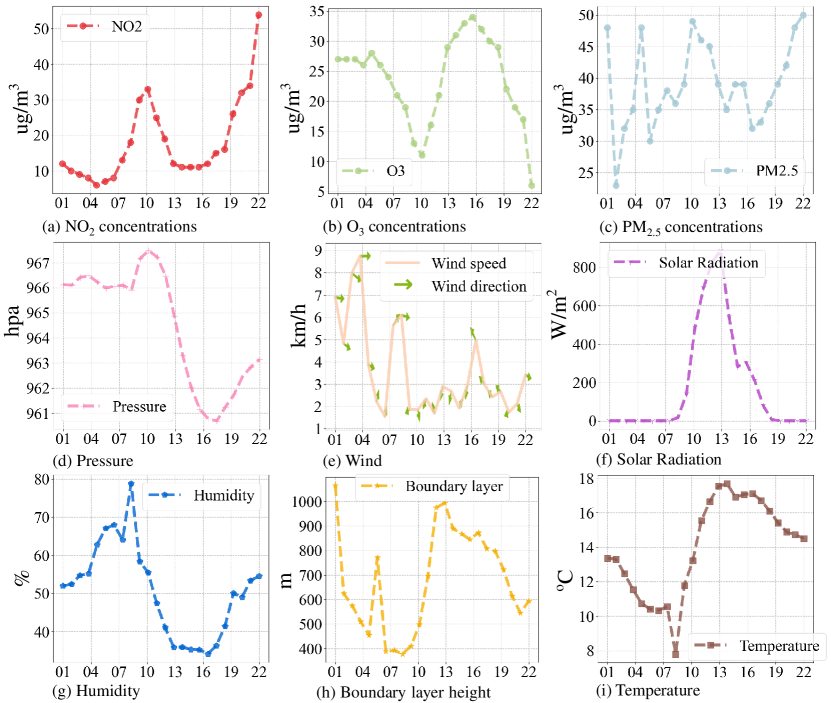
Figure Appendix 2. Pollutant concentrations and meteorological conditions during Mar. 1, 2022

Previous studies have shown that meteorological conditions significantly affect pollutant concentrations (ZYFH2013, ; MMMM2023, ). The relationship between meteorological conditions and the concentrations of NO₂, O₃, and PM_2.5 is further explored in Fig. Appendix 2. For instance, on Mar. 1, 2023, at 4:00 AM, conditions such as low boundary layer height and solar radiation, medium temperature and humidity, high pressure and wind speed correspond to low NO₂ concentrations, high O₃ concentrations, and medium PM_2.5 concentrations. Considering the impact of wind direction on pollutant diffusion direction (SXWHQ2021, ), seven meteorological factors ($X^{\text{ME}}$) are finally selected as features for air quality inference: boundary layer height, temperature, humidity, pressure, wind speed, wind direction, and solar radiation.

Appendix A.3. Traffic data

Traffic has been identified as a major contributor to air pollutant emissions. Specifically, Karagulian et al. (KFBCDC2015, ) show that traffic is responsible for approximately 25% of $PM$ emissions, and Baldasano et al. (BJ2020, ) note that traffic emissions account for about 65% of total NO₂ emissions. Consequently, three types of traffic-related features are designed for air quality inference: the origin-destination adjacency matrix ($A^{\text{OD}}$), derived from the movement patterns of construction waste trucks; the grid congestion index ($X^{\text{CI}}$), calculated based on road congestion; and construction waste truck flow ($X^{\text{FL}}$), determined from the trajectory points of construction waste trucks.

OD adjacency matrix ($A^{\text{OD}}$): Due to the lack of modern exhaust treatment systems, heavy-duty diesel vehicles emit more air pollutants than other vehicles (APJJ2011, ), making them a major source of traffic air pollutants (KFCCPASHM2015, ; JPXL2020, ). Specifically, in China, heavy-duty diesel vehicles account for 70.4% of $NO_{x}$ emissions and 51.9% of $PM_{x}$ emissions from all vehicle types (HYCLZLW2023, ). Among the heavy-duty diesel vehicles, construction waste trucks are one of the most common vehicles. Consequently, an OD adjacency matrix ($A^{\text{OD}}$) is designed to approximate the spatial dependency of traffic-related pollutant emissions using the movement patterns of construction waste trucks, a type of diesel-powered vehicle. Specifically, the trajectory points of these trucks are employed to obtain the one-hop origin-destination relationship (OHODR) between the grids, as shown in Fig. Appendix 3. Subsequently, $A^{\text{OD}}$ can be defined as follows:

(Appendix 1) $$A^{\text{OD}}\left(i,j\right)=\begin{cases}1,\text{ if }r_{i}\text{ and }r_{j}\text{ have OHODR}\\ 0,\text{ otherwise}\\ \end{cases}$$

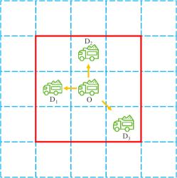
Figure Appendix 3. One-hop OD relationship between grids, with the red box indicating regions where this relationship exists.

Construction waste truck flow ($X^{\text{FL}}$): Construction waste trucks are known for generating on-road and on-site fugitive dust, which is a significant contributor to atmospheric particulate matter (WHHLTQZFSTHJ2023, ). Consequently, construction waste truck flow ($X^{\text{FL}}$) is used as a feature for PM_2.5 concentration inference.

Grid congestion index ($X^{\text{CI}}$): Pollutant emissions escalate on congested roadways due to increased idling and more frequent accelerations of vehicles (AKHAM2002, ; CCBWMJ2005, ). Furthermore, the relationship between pollutant concentration fluctuations and traffic congestion exhibits a positive cross-correlation (SKBKCL2018, ). Consequently, the grid congestion index ($X^{\text{CI}}$) is proposed and defined as follows:

(Appendix 2) $$X_{t,i}^{CI}=\frac{\sum_{l_{j,i}\in r_{i}}{c_{t,j}l_{j,i}}}{\sum_{l_{j,i}\in r_{i}}{l_{j,i}}}$$

where $X_{t,i}^{\text{CI}}$ identifies the grid congestion index of $r_{i}$ at timestamp $t$, $c_{t,j}$ represents the congestion index of road $j$ at the same time, and $l_{j,i}$ indicates the length of road $j$ within the grid $r_{i}$.

Appendix A.4. Geographic data

Air pollutant concentrations are closely associated with land usage and function, which can be characterized through geographic data. Consequently, two types of features are designed: geographic features ($X^{\text{GE}}$) and the semantic adjacency matrix ($A^{\text{SE}}$), constructed based on the similarity of $X^{\text{GE}}$.

Geographic features $X^{\text{GE}}$: $X^{\text{GE}}$ contains three main types of features: POI features ($X^{\text{POI}}$), land use features ($X^{\text{LU}}$), and road length features ($X^{\text{RL}}$). More details can be found in Table Appendix 1.

Table Appendix 1. Details of $X^{\text{POI}}$, $X^{\text{LU}}$ and $X^{\text{RL}}$.

Feature type	Details
$X^{\text{POI}}$	Culture and education, Financial institutions
	Food and beverage, Shopping malls
	Companies, Transportation spots, Hospitals
	Traveling spots, Hotels, Stadiums
	Residential buildings, Vehicle Services
$X^{\text{LU}}$	Traffic route, Tree cover, Water
	Grassland, Cropland, Buildings, Sparse vegetation
$X^{\text{RL}}$	Trunk, Trunk link, Primary
	Primary link, Secondary
	Secondary link, Tertiary, Tertiary link

Semantic adjacency matrix ($A^{\text{SE}}$): Grids with similar geographical features tend to exhibit comparable pollutant concentrations. For example, grids with a similar number of factories might have similar pollutant concentrations. Consequently, semantic adjacency matrix ($A^{\text{SE}}$) is designed. Specifically, K-means (KKM1999, ) is employed to cluster grids based on their $X^{\text{GE}}$, and $A^{\text{SE}}$ is defined as follows:

(Appendix 3) $$A^{\text{SE}}\left(i,j\right)=\begin{cases}1,\text{ if }r_{i}\text{ and }r_{j}\text{ in the same cluster}\\ 0,\text{ otherwise}\\ \end{cases}$$

Appendix A.5. Timestamp data

Fig. Appendix 4 presents the power spectral density (PSD) of seasonalities, revealing the partial periodic patterns of pollutant concentrations. Consequently, features representing hour of day ($X^{\text{HD}}$) and day of week ($X^{\text{DW}}$) are extracted from timestamps to capture the daily and weekly patterns respectively, which are commonly employed to infer pollutant concentrations. Notably, $X^{\text{HD}}$ and $X^{\text{DW}}$ are the only two categorical features used in this paper.

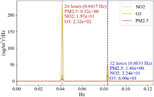
Figure Appendix 4. The power spectral density (PSD) of the seasonality for NO₂, O₃ and PM_2.5. Each peak denotes a periodicity.

Appendix A.6. Data summary

In conclusion, one type of label and ten types of features are aggregated, which could further divided into 42 subcategories, as detailed in the Table Appendix 2.

Table Appendix 2. Data summary

Type	Name	Element Description
$X_{\text{num}}$	$X^{\text{TRL}}$	Trend data extracted from micro-stations
	$X^{\text{REP}}$	Most relevant pollutant concentrations after spatial interpolation.
		For O3, NO2, and PM2.5, the most relevant pollutants
		are NO2, O3, and NO2, respectively.
	$X^{\text{ME}}$	Boundary layer height $X^{\text{BLH}}$, Temperature $X^{\text{TE}}$
		Humidity $X^{\text{HU}}$, Pressure $X^{\text{PR}}$, Wind speed $X^{\textbf{WS}}$
		Wind direction $X^{\text{WD}}$, Solar radiation $X^{\text{SR}}$
	$X^{\text{CI}}$	Grid congestion index
	$X^{\text{GE}}$	POI, Land use, Road length
	$X^{\text{FL}}$	Construction waste truck flow
$X_{\text{cat}}$	$X^{\text{HD}}$	Hour of day
	$X^{\text{DW}}$	Day of week
$\bm{A}$	$A^{\text{OD}}$	OD adjacency matrix
	$A^{\text{SE}}$	Semantic adjacency matrix
$Y$	$Y_{c}$	Target pollutant concentrations from standardized stations

Appendix Appendix B Experiments

Appendix B.1. Experimental Settings

Fig. Appendix 5 report the detail hyperparameter settings of MTSTN’s architecture.

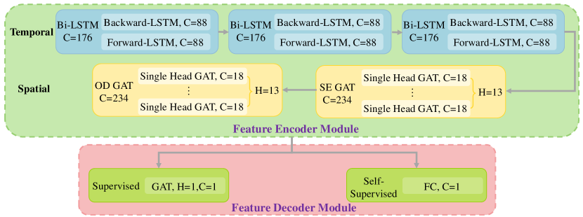
Figure Appendix 5. Hyperparameter settings of MTSTN.

Appendix B.2. Hyperparameter Study

A systematic investigation into the performance of MTSTN under different hyperparameter settings is conducted. In each experiment, a single hyperparameter is modified while the others remain unchanged as the default settings, thereby isolating the effects of other parameters. Notably, although each hyperparameter is incrementally increased from its minimum value, only the critical results are presented in this paper.

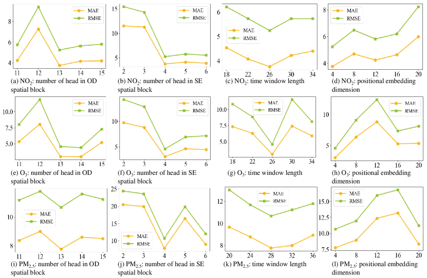
Figure Appendix 6. The performance of MTSTN under different parameter settings.

Appendix B.2.1. Effects of number of head in graph attention layers

The number of heads in the graph attention layers of the OD and SE spatial blocks are adjusted, and the results for MAE and RMSE are reported in Fig. Appendix 6 (a)-(b), (e)-(f), and (i)-(j). When MTSTN’s performance peaks, OD spatial block employs more heads than SE spatial block, suggesting greater complexity within $A^{OD}$.

Appendix B.2.2. Effects of time window length

As shown in Fig. Appendix 6 (c), (g), and (k), the errors of MTSTN exhibit a downward trend until $\tau$ reaches 26 or 28, after which they begin to increase. This phenomenon suggests that longer time windows cannot guarantee better results.

Appendix B.2.3. Effects of positional embedding dimension

Finally, the positional embedding dimension $d_{p}$ is modified. As shown in Fig. Appendix 6 (d), (h), and (l), an increase in $d_{p}$ leads to a decline in MTSTN’s performance. This decline may be attributed to the increased distance between data points in higher dimensions, which hinders MTSTN’s ability to capture the data’s local structure.

Appendix B.3. Baselines

MTSTN is compared with nine baselines, which can be categorized into interpolation models, machine learning models, and deep learning models. Further details about the baselines are provided below.

• KNN: K-Nearest Neighbors estimates the unknown nodes by interpolating the readings of the K closest nodes (HJYZLYR2023, ).

• IDW: Inverse Distance Weighting is a deterministic interpolation method that infers unknown nodes using the weighted averages of nearby available nodes, with closer nodes having more influence (LGD2008, ).

• LUR: Land Use Regression utilizes related exogenous covariates, such as land use and traffic characteristics, to estimate pollutant concentrations for unknown nodes (HDOCCML2014, ).

• RF: Random forest is extensively used and recognized for its efficient performance in handling non-linear regression tasks (FKME2014, ).

• XGBoost: Extreme Gradient Boosting is an efficient and scalable machine learning algorithm known for its superior performance in both classification and regression tasks (CTGC2016, ).

• STGCN: Spatio-Temporal Graph Convolutional Networks is a purely convolutional structure that enables faster training with fewer parameters (YBHZ2017, ).

• MSTGCN: Multi-View Spatial-Temporal Graph Convolutional Networks not only capture the most relevant spatio-temporal information but also exhibit strong domain generalization capabilities (JZYJXYRYH2021, ).

• ASTGNN: Attention-based Spatial-Temporal Graph Neural Network efficiently captures temporal dynamics, spatial dynamics, and spatial heterogeneity through a novel self-attention mechanism (GSYHX2021, ).

• PDFormer: Propagation Delay-Aware Dynamic Long-Range Transformer is one of the state-of-the-art spatio-temporal prediction model, capable of capturing delayed propagation (JJCWJ2023, ).

References

- (1) Xia Meng, Cong Liu, Renjie Chen, Francesco Sera, Ana Maria Vicedo-Cabrera, Ai Milojevic, Yuming Guo, Shilu Tong, Micheline de Sousa Zanotti Stagliorio Coelho, Paulo Hilario Nascimento Saldiva, et al. 2021. Short term associations of ambient nitrogen dioxide with daily total, cardiovascular, and respiratory mortality: multilocation analysis in 398 cities. bmj 372 (2021).
- (2) Daniel A Vallero. 2014. Fundamentals of air pollution. Academic press.
- (3) Joshua S Apte, Kyle P Messier, Shahzad Gani, Michael Brauer, Thomas W Kirchstetter, Melissa M Lunden, Julian D Marshall, Christopher J Portier, Roel CH Vermeulen, and Steven P Hamburg. 2017. High-resolution air pollution mapping with Google street view cars: exploiting big data. Environmental science & technology 51, 12 (2017), 6999–7008.
- (4) Junfeng Hu, Yuxuan Liang, Zhencheng Fan, Li Liu, Yifang Yin, and Roger Zimmermann. 2023. Decoupling long-and short-term patterns in spatiotemporal inference. IEEE Transactions on Neural Networks and Learning Systems (2023).
- (5) Weiyu Cheng, Yanyan Shen, Yanmin Zhu, and Linpeng Huang. 2018. A neural attention model for urban air quality inference: Learning the weights of monitoring stations. In Proceedings of the AAAI conference on artificial intelligence, Vol. 32.
- (6) Roger Zimmermann. 2023. Graph Neural Processes for Spatio-Temporal Extrapolation. In Proceedings of the 29th ACM SIGKDD Conference on Knowledge Discovery and Data Mining.
- (7) Ling Chen, Yaya Cai, Yifang Ding, Mingqi Lv, Cuili Yuan, and Gencai Chen. 2016. Spatially fine-grained urban air quality estimation using ensemble semi-supervised learning and pruning. In Proceedings of the 2016 ACM international joint conference on pervasive and ubiquitous computing. 1076–1087.
- (8) Yu Zheng, Furui Liu, and Hsun-Ping Hsieh. 2013. U-air: When urban air quality inference meets big data. In Proceedings of the 19th ACM SIGKDD international conference on Knowledge discovery and data mining. 1436–1444.
- (9) Tobias Ross, David Zimmerer, Anant Vemuri, Fabian Isensee, Manuel Wiesenfarth, Sebastian Bodenstedt, Fabian Both, Philip Kessler, Martin Wagner, Beat Müller, et al. 2018. Exploiting the potential of unlabeled endoscopic video data with self-supervised learning. International journal of computer assisted radiology and surgery 13 (2018), 925–933.
- (10) Wei Jin, Tyler Derr, Haochen Liu, Yiqi Wang, Suhang Wang, Zitao Liu, and Jiliang Tang. 2020. Self-supervised learning on graphs: Deep insights and new direction. arXiv preprint arXiv:2006.10141 (2020).
- (11) Robert B Cleveland, William S Cleveland, Jean E McRae, and Irma Terpenning. 1990. STL: A seasonal-trend decomposition. J. Off. Stat 6, 1 (1990), 3–73.
- (12) Yury Gorishniy, Ivan Rubachev, Valentin Khrulkov, and Artem Babenko. 2021. Revisiting deep learning models for tabular data. Advances in Neural Information Processing Systems 34 (2021), 18932–18943.
- (13) T Cover. 1968. Estimation by the nearest neighbor rule. IEEE Transactions on Information Theory 14, 1 (1968), 50–55.
- (14) Patrick M Bartier and C Peter Keller. 1996. Multivariate interpolation to incorporate thematic surface data using inverse distance weighting (IDW). Computers & Geosciences 22, 7 (1996), 795–799.
- (15) David J Briggs, Susan Collins, Paul Elliott, Paul Fischer, Simon Kingham, Erik Lebret, Karel Pryl, Hans Van Reeuwijk, Kirsty Smallbone, and Andre Van Der Veen. 1997. Mapping urban air pollution using GIS: a regression-based approach. International Journal of Geographical Information Science 11, 7 (1997), 699–718.
- (16) Leo Breiman. 2001. Random forests. Machine learning 45 (2001), 5–32.
- (17) Tianqi Chen, Tong He, Michael Benesty, Vadim Khotilovich, Yuan Tang, Hyunsu Cho, Kailong Chen, Rory Mitchell, Ignacio Cano, Tianyi Zhou, et al. 2015. Xgboost: extreme gradient boosting. R package version 0.4-2 1, 4 (2015), 1–4.
- (18) Bing Yu, Haoteng Yin, and Zhanxing Zhu. 2017. Spatio-temporal graph convolutional networks: A deep learning framework for traffic forecasting. arXiv preprint arXiv:1709.04875 (2017).
- (19) Ziyu Jia, Youfang Lin, Jing Wang, Xiaojun Ning, Yuanlai He, Ronghao Zhou, Yuhan Zhou, and H Lehman Li-wei. 2021. Multi-view spatial-temporal graph convolutional networks with domain generalization for sleep stage classification. IEEE Transactions on Neural Systems and Rehabilitation Engineering 29 (2021), 1977–1986.
- (20) Shengnan Guo, Youfang Lin, Huaiyu Wan, Xiucheng Li, and Gao Cong. 2021. Learning dynamics and heterogeneity of spatial-temporal graph data for traffic forecasting. IEEE Transactions on Knowledge and Data Engineering 34, 11 (2021), 5415–5428.
- (21) Jiawei Jiang, Chengkai Han, Wayne Xin Zhao, and Jingyuan Wang. 2023. Pdformer: Propagation delay-aware dynamic long-range transformer for traffic flow prediction. In Proceedings of the AAAI conference on artificial intelligence, Vol. 37. 4365–4373.
- (22) Mei-Yi Fan, Yan-Lin Zhang, Yu-Chi Lin, Yihang Hong, Zhu-Yu Zhao, Feng Xie, Wei Du, Fang Cao, Yele Sun, and Pingqing Fu. 2021. Important role of NO3 radical to nitrate formation aloft in urban Beijing: Insights from triple oxygen isotopes measured at the tower. Environmental Science & Technology 56, 11 (2021), 6870–6879.
- (23) Chao Yan, Yee Jun Tham, Wei Nie, Men Xia, Haichao Wang, Yishuo Guo, Wei Ma, Junlei Zhan, Chenjie Hua, Yuanyuan Li, et al. 2023. Increasing contribution of nighttime nitrogen chemistry to wintertime haze formation in Beijing observed during COVID-19 lockdowns. Nature Geoscience 16, 11 (2023), 975–981.
- (24) Ann Carine Vandaele, Christian Hermans, Sophie Fally, Michel Carleer, Réginald Colin, M-F Merienne, Alain Jenouvrier, and Bernard Coquart. 2002. Highresolution Fourier transform measurement of the NO2 visible and near-infrared. absorption cross sections: Temperature and pressure effects. Journal of Geophysical Research: Atmospheres 107, D18 (2002), ACH–3.
- (25) Daniel L Goldberg, Susan C Anenberg, Gaige Hunter Kerr, Arash Mohegh, Zifeng Lu, and David G Streets. 2021. TROPOMI NO2 in the United States: A detailed look at the annual averages, weekly cycles, effects of temperature, and correlation with surface NO2 concentrations. Earth’s future 9, 4 (2021), e2020EF001665.
- (26) Yuning You, Tianlong Chen, Zhangyang Wang, and Yang Shen. 2020. When does self-supervision help graph convolutional networks. In international conference on machine learning. PMLR, 10871–10880.
- (27) Kaiming He, Xinlei Chen, Saining Xie, Yanghao Li, Piotr Dollár, and Ross Girshick. 2022. Masked autoencoders are scalable vision learners. In Proceedings of the IEEE/CVF conference on computer vision and pattern recognition. 16000–16009.
- (28) Ashish Vaswani, Noam Shazeer, Niki Parmar, Jakob Uszkoreit, Llion Jones, Aidan N Gomez, Łukasz Kaiser, and Illia Polosukhin. 2017. Attention is all you need. Advances in neural information processing systems 30 (2017).
- (29) Xiaotong Sun, Wei Xu, Hongxun Jiang, and Qili Wang. 2021. A deep multitask learning approach for air quality prediction. Annals of Operations Research 303 (2021), 51–79.
- (30) George Y Lu and David W Wong. 2008. An adaptive inverse-distance weighting spatial interpolation technique. Computers & geosciences 34, 9 (2008), 1044–1055.
- (31) Mike Schuster and Kuldip K Paliwal. 1997. Bidirectional recurrent neural networks. IEEE transactions on Signal Processing 45, 11 (1997), 2673–2681.
- (32) Petar Velickovic, Guillem Cucurull, Arantxa Casanova, Adriana Romero, Pietro Lio, Yoshua Bengio, et al. 2017. Graph attention networks. stat 1050, 20 (2017), 10–48550.
- (33) Lynette J Clapp and Michael E Jenkin. 2001. Analysis of the relationship between ambient levels of O3, NO2 and NO as a function of NOx in the UK. Atmospheric Environment 35, 36 (2001), 6391–6405.
- (34) Paul J Crutzen. 1979. The role of NO and NO2 in the chemistry of the troposphere and stratosphere. Annual review of earth and planetary sciences 7, 1 (1979), 443–472.
- (35) Suqin Han, Hai Bian, Yinchang Feng, Aixia Liu, Xiangjin Li, Fang Zeng, Xiaoling Zhang, et al. 2011. Analysis of the relationship between O3, NO and NO2 in Tianjin, China. Aerosol and Air Quality Research 11, 2 (2011), 128–139.
- (36) Manuel Méndez, Mercedes G Merayo, and Manuel Núñez. 2023. Machine learning algorithms to forecast air quality: a survey. Artificial Intelligence Review 56, 9 (2023), 10031–10066.
- (37) Federico Karagulian, Claudio A Belis, Carlos Francisco C Dora, Annette M PrüssUstün, Sophie Bonjour, Heather Adair-Rohani, and Markus Amann. 2015. Contributions to cities’ ambient particulate matter (PM): A systematic review of local source contributions at global level. Atmospheric environment 120 (2015), 475–483.
- (38) José M Baldasano. 2020. COVID-19 lockdown effects on air quality by NO2 in the cities of Barcelona and Madrid (Spain). Science of the Total Environment 741 (2020), 140353.
- (39) Pia Anttila, Juha-Pekka Tuovinen, and Jarkko V Niemi. 2011. Primary NO2 emissions and their role in the development of NO2 concentrations in a traffic environment. Atmospheric Environment 45, 4 (2011), 986–992.
- (40) Federico Karagulian, Claudio A Belis, Carlos Francisco C Dora, Annette M PrüssUstün, Sophie Bonjour, Heather Adair-Rohani, and Markus Amann. 2015. Contributions to cities’ ambient particulate matter (PM): A systematic review of local source contributions at global level. Atmospheric environment 120 (2015), 475–483.
- (41) Peiyu Jiang, Xi Zhong, and Lingyu Li. 2020. On-road vehicle emission inventory and its spatio-temporal variations in North China Plain. Environmental Pollution 267 (2020), 115639.
- (42) Ke Han, YANG Zhuoqian, CHEN Caiyun, LIU Xiaobo, ZHAO Bin, LI Wei, and WANG Yongdong. 2023. Intelligent management and emission reduction of construction waste hauling trucks – a Chengdu case Study. Preprint (2023).
- (43) Haibin Wang, Lihui Han, Tingting Li, Song Qu, Yuncheng Zhao, Shoubin Fan, Tong Chen, Haoran Cui, and Junfang Liu. 2023. Temporal-spatial distributions of road silt loadings and fugitive road dust emissions in Beijing from 2019 to 2020. Journal of Environmental Sciences 132 (2023), 56–70.
- (44) Kyoungho Ahn, Hesham Rakha, Antonio Trani, and Michel Van Aerde. 2002. Estimating vehicle fuel consumption and emissions based on instantaneous speed and acceleration levels. Journal of transportation engineering 128, 2 (2002), 182–190.
- (45) Christina A Colberg, Bruno Tona, Werner A Stahel, Markus Meier, and Johannes Staehelin. 2005. Comparison of a road traffic emission model (HBEFA) with emissions derived from measurements in the Gubrist road tunnel, Switzerland. Atmospheric Environment 39, 26 (2005), 4703–4714.
- (46) Kai Shi, Baofeng Di, Kaishan Zhang, Chaoyang Feng, and Laurence Svirchev. 2018. Detrended cross-correlation analysis of urban traffic congestion and NO2 concentrations in Chengdu. Transportation Research Part D: Transport and Environment 61 (2018), 165–173.
- (47) K Krishna and M Narasimha Murty. 1999. Genetic K-means algorithm. IEEE Transactions on Systems, Man, and Cybernetics, Part B (Cybernetics) 29, 3 (1999), 433–439.
- (48) David Hasenfratz, Olga Saukh, Christoph Walser, Christoph Hueglin, Martin Fierz, and Lothar Thiele. 2014. Pushing the spatio-temporal resolution limit of urban air pollution maps. In 2014 IEEE International Conference on Pervasive Computing and Communications (PerCom). IEEE, 69–77.
- (49) Khaled Fawagreh, Mohamed Medhat Gaber, and Eyad Elyan. 2014. Random forests: from early developments to recent advancements. Systems Science & Control Engineering: An Open Access Journal 2, 1 (2014), 602–609.
- (50) Tianqi Chen and Carlos Guestrin. 2016. Xgboost: A scalable tree boosting system. In Proceedings of the 22nd acm sigkdd international conference on knowledge discovery and data mining. 785–794.
1