A Unified Framework for Interpretable Transformers Using PDEs and Information Theory

Abstract

This paper presents a novel unified theoretical framework for understanding and analyzing Transformer architectures by integrating Partial Differential Equations (PDEs), Neural Information Flow Theory, and Information Bottleneck Theory. We model the information dynamics in Transformers as a continuous PDE process, encompassing diffusion, self-attention, and nonlinear residual components. To validate our approach, we conduct comprehensive experiments across image and text modalities, including information flow visualization, attention mechanism analysis, information bottleneck effect validation, gradient flow analysis, and perturbation sensitivity analysis. Our results demonstrate that the PDE model effectively captures key aspects of Transformer behavior, achieving high similarity (cosine similarity > 0.98) with Transformer attention distributions across all layers.This work provides new theoretical insights into Transformer mechanisms, offering a foundation for future optimizations in deep learning architecture design. We discuss the implications of our findings and outline directions for enhancing PDE models to better mimic the complex behaviors observed in Transformers

1 Introduction

1.1 background

The Transformer modelVaswani (2017) has emerged as a cornerstone technology in the field of Natural Language Processing (NLP), revolutionizing the way machines understand and generate human language. Since its introduction, the Transformer architecture has been at the heart of numerous state-of-the-art systems, excelling in tasks such as machine translation, text summarization, and text generation. Its ability to handle long-range dependencies in text and efficiently parallelize computations has made it the preferred choice for developing advanced NLP applications.

Despite their widespread success, Transformers present significant challenges in terms of interpretability. The model’s multi-layered architecture, combined with the self-attention mechanism, creates a complex system where information flows and transformations occur in a highly non-linear and dynamic manner. This complexity makes it difficult to fully understand how input information is processed and how specific outputs are generated. Current interpretability methods, while useful, often fall short in providing a comprehensive explanation of the internal workings of Transformers, particularly in terms of how information is propagated and modified across different layers and attention heads within the model.

1.2 Relevant Literature

Transformer models have achieved significant success in natural language processing and computer vision but face challenges in explainability, particularly in fields like healthcare and law where transparency is critical Zini and Awad (2022). To address this, recent research has developed explainability methods across three levels: input (e.g., word embeddings), processing (e.g., attention mechanisms), and output (e.g., model decisions) Zini and Awad (2022); Kashefi et al. (2023). Deep Taylor Decomposition and Layer-wise Relevance Propagation (LRP) are among the approaches that improve interpretability over traditional gradient-based methods Chefer et al. (2021); Ali et al. (2022). Alternatives to attention mechanisms, such as attention flow and attention rollout, have been proposed to better quantify token relevance Abnar and Zuidema (2020); Metzger et al. (2022), while tools like Ecco Alammar (2021) offer interactive ways to explore model behavior.

In specific domains, explainability methods have been applied to tasks such as gene transcription analysis in genomics Clauwaert et al. (2021); Graça et al. (2023), sentiment analysis Fiok et al. (2021), and dynamic user representations in collaborative filtering Gaiger et al. (2023). Visualizing patch interactions in vision transformers Ma et al. (2023) and tracking transformers with class and regression tokens have further expanded the understanding of attention mechanisms in these models Di Nardo and Ciaramella (2023). Gradient-based approaches continue to play a crucial role in explaining transformer models across diverse fields, improving diagnostic accuracy in medical applications like ECG interpretation Vaid et al. (2023); Poulton and Eliens (2021); Lundberg and Lee (2017). Despite these advancements, a unified framework for evaluating explainability methods is still needed Zini and Awad (2022); Kashefi et al. (2023).

1.3 Research Motivation and Objectives

Current interpretability methods for Transformer models largely rely on discrete approximations or empirical observations, but they fail to capture the continuous, dynamic processes of information flow within these models. These methods do not adequately address how information propagates through Transformer layers, limiting a deeper understanding of their internal mechanisms. This lack of a theoretical framework constrains efforts to optimize model stability and performance, particularly in high-stakes applications where reliability is critical. As Transformers are increasingly applied in such contexts, there is a pressing need for a more rigorous and continuous approach that can explain both deterministic and stochastic elements of information processing.

The objective of this research is to develop a unified mathematical model that integrates Partial Differential Equations (PDEs), Neural Information Flow Theory, and Information Bottleneck Theory to provide a comprehensive understanding of Transformer behavior. By focusing on information flow, this model seeks to enhance the interpretability of Transformers, optimize their architecture, and improve their stability and efficiency. The ultimate goal is to contribute to the design of more robust and interpretable AI systems that can perform reliably in complex environments.

1.4 Our Contributions and the Structure of the Paper

This paper introduces a novel unified theoretical framework that integrates Partial Differential Equations (PDEs), Neural Information Flow Theory, and Information Bottleneck Theory to provide a continuous and rigorous explanation of Transformer models. Unlike previous approaches that focus on discrete or empirical observations, our framework emphasizes the dynamic information flow within Transformer layers, offering deeper insights into how information is processed and transformed. This framework bridges the gap between empirical observations and theoretical understanding, paving the way for new strategies in Transformer architecture optimization, improving both stability and efficiency. The framework is validated through extensive experiments, showing its potential to develop more interpretable, robust, and efficient AI systems.

The structure of the paper is as follows:

• Section 2: Methodology This section outlines the theoretical basis, focusing on the integration of PDEs, Neural Information Flow Theory, and Information Bottleneck Theory. We introduce mathematical models that explain Transformer dynamics, particularly through PDE-inspired mechanisms, and detail a multi-layer information flow framework.

• Section 3: Experimental Results We conduct five key experiments to validate the proposed framework. These experiments cover information flow visualization, attention mechanism analysis, information bottleneck effect validation, gradient flow analysis, and perturbation sensitivity analysis. Results demonstrate that the PDE-based model effectively captures essential behaviors of Transformer models, particularly in terms of information propagation and stability.

2 Methodology

2.1 Theoretical Foundation

2.1.1 Neural Information Flow Theory

Neural Information Flow Theory focuses on how information is transmitted and transformed across different layers of neural networksGoldfeld et al. (2018); Stone (2018). It provides a framework for understanding how networks distill raw input into meaningful features, preserving relevant information while discarding unnecessary details. This theory highlights the layer-wise propagation of information and offers insights into optimizing network architectures for better performance and interpretability by tracking the flow of information throughout the model.

2.1.2 Partial Differential Equations (PDEs)

Partial Differential Equations (PDEs) are mathematical tools used to describe the continuous behavior of complex systems. In the analysis of Transformer models, PDEs allow us to model the flow of information as a continuous process, offering a nuanced perspective on how information evolves over time and across layers. By leveraging PDEs, we can better understand the intricate dynamics of information transmission and transformation, leading to deeper insights and potential improvements in Transformer architecture design.

2.1.3 Information Bottleneck Theory

Information Bottleneck Theory addresses the trade-off between compressing input data and retaining information necessary for accurate predictions.Tishby et al. (2000)It provides a framework for understanding how neural networks focus on relevant information while discarding redundancy. In the context of Transformers, this theory helps explain how models efficiently process information across layers, enhancing interpretability and generalization by balancing compression with predictive accuracy.

2.2 Mathematical Model

We present a novel, unified mathematical framework that integrates Partial Differential Equations (PDEs), Neural Information Flow Theory, and Information Bottleneck Theory to provide a comprehensive explanation of the Transformer architecture. This approach offers new insights into the intricate dynamics of information processing within Transformers, bridging the gap between empirical success and theoretical understanding.

2.2.1 PDE-Inspired Transformer Dynamics

When analyzing Transformer behavior, the Partial Differential Equation (PDE) model provides a continuous, physics-based perspective. By modeling information flow as a PDE process, we can integrate diffusion terms, self-attention mechanisms, and nonlinear residual components into a single equation to capture the propagation and transformation of information within Transformers. This approach not only offers a rigorous mathematical framework for understanding the dynamics of information flow but also bridges the gap between empirical observations and theoretical foundations. Through this integration, the PDE model enables a more nuanced and comprehensive analysis of the mechanisms underpinning Transformer architectures, providing valuable insights into their operational principles and potential avenues for optimization.

The cornerstone of our model is a PDE-inspired formulation that captures the essence of information flow in Transformers:

$$\frac{\partial u}{\partial t}=D\nabla^{2}u+\alpha A(u)+R(u,\theta,t,x)$$ (1)

where:

• $u(x,t)\in\mathbb{R}^{d}$ represents the $d$-dimensional embedding of the token at position $x$ and time $t$.

• $D\nabla^{2}u$ is the diffusion term, with $D\in\mathbb{R}^{d\times d}$ being the diffusion tensor, and $\nabla^{2}$ the Laplacian operator, modeling the global context integration in Transformers.

• $A(u)$ is the self-attention mechanism, defined as:

  $$A(u)=\text{Softmax}\left(\frac{Q(u)K(u)^{T}}{\sqrt{d_{k}}}\right)V(u)$$ (2)

  where $Q(u)=W_{Q}u$, $K(u)=W_{K}u$, and $V(u)=W_{V}u$ are the query, key, and value projections, respectively, with $W_{Q},W_{K},W_{V}\in\mathbb{R}^{d\times d}$, and $d_{k}$ is the dimensionality of the key vectors.

• $\alpha\in\mathbb{R}^{+}$ is the attention strength coefficient, analogous to the scaling factor in Transformer attention.

• $R(u,\theta,t,x)$ is the nonlinear residual term, encompassing the feed-forward networks and residual connections in Transformers.

This formulation provides several key advantages in analyzing Transformer behavior: modeling token embeddings as a continuous field $u(x,t)$ enables the application of powerful PDE analysis techniques to understand information propagation in Transformers; interpreting the attention mechanism as a form of directed, content-dependent diffusion offers a novel perspective on how Transformers integrate contextual information; and incorporating both spatial ($x$) and temporal ($t$) dimensions allows for the analysis of how information evolves within a sequence and through the layers of the network.

2.2.2 Information Bottleneck in Transformer Learning

The Information Bottleneck (IB) theory provides a powerful framework for understanding the learning processes of deep learning models. In the context of Transformers, this theory can help elucidate how the model balances retaining task-relevant information and compressing input representations. By integrating the IB theory into our PDE model, we can delve into the information dynamics during Transformer training, including representation efficiency, regularization effects, and the trade-off between task performance and information compression. To capture these dynamics in the learning process of Transformers, we introduce the following equation:

$$\frac{\partial\theta}{\partial t}=-\nabla_{\theta}L(\theta)+\lambda\theta-\beta\nabla_{\theta}I(X;T_{\theta}(X))$$ (3)

where:

• $L(\theta)$ is the task-specific loss function.

• $\lambda\theta$ represents the L2 regularization term, commonly used in Transformer training.

• $I(X;T_{\theta}(X))$ is the mutual information between input $X$ and its Transformer representation $T_{\theta}(X)$.

• $\beta\in\mathbb{R}^{+}$ is the hyperparameter balancing task performance and information compression.

This formulation allows us to explore how Transformers optimize the encoding of input data to retain essential information for specific tasks while minimizing redundancy. By minimizing the mutual information term $I(X;T_{\theta}(X))$, the model is encouraged to learn compact, task-relevant representations, thus explaining the effectiveness of Transformers across various tasks. The regularization term acts as a form of regularization, potentially enhancing the generalization capabilities of Transformers. Moreover, the $\beta$ parameter provides explicit control over the trade-off between task performance and representation compression, offering a new avenue for fine-tuning model performance. This integrated approach not only deepens our theoretical understanding of Transformer learning dynamics but also guides the development of more efficient and robust Transformer architectures.

2.2.3 Multi-Layer Information Flow in Transformers

The multi-layer structure of Transformers is fundamental to their powerful capabilities. Each layer transforms and refines the input information, progressively building more abstract and task-specific representations. To comprehensively understand this process, a model that can describe the information flow between layers is essential. Our multi-scale PDE framework not only captures the information processing within individual layers but also simulates the interactions between layers, including the effects of residual connections and layer normalization. This enables us to conduct hierarchical analysis, examining the specific behaviors of different layers and their contributions to the overall performance of the model. Based on this concept, we extend our framework to the following multi-layer information flow mode

$$\frac{\partial u_{l}}{\partial t}=D_{l}\nabla^{2}u_{l}+\alpha_{l}A_{l}(u_{l})+R_{l}(u_{l},\theta_{l},t,x)+C_{l-1,l}(u_{l-1})-C_{l,l+1}(u_{l})$$ (4)

where:

• $u_{l}(x,t)$ represents the information state at layer $l$, position $x$, and time $t$.

• $D_{l}\nabla^{2}u_{l}$ is the layer-specific diffusion term.

• $A_{l}(u_{l})$ is the self-attention mechanism for layer $l$, defined analogously to Equation 2.

• $R_{l}(u_{l},\theta_{l},t,x)$ is the layer-specific nonlinear residual term.

• $C_{l-1,l}(u_{l-1})$ and $C_{l,l+1}(u_{l})$ are inter-layer communication operators, modeling residual connections and layer normalization effects.

This multi-scale formulation offers several advantages, including the ability to conduct hierarchical analysis of how information is processed and transformed across different layers of the Transformer, insights into inter-layer interactions through the terms $C_{l-1,l}$ and $C_{l,l+1}$, which capture the effects of skip connections and allow for analysis of information flow between adjacent layers, and the examination of layer-specific behaviors by incorporating layer-specific parameters ($D_{l}$, $\alpha_{l}$, etc.), thereby analyzing the contributions of different layers to the overall information processing in Transformers.

2.2.4 Mathematical Model Algorithm

Algorithm 1 presents the main procedure of our proposed simplified mathematical model, which integrates partial differential equations (PDEs) with key components of Transformer architectures. This algorithm encapsulates the core concepts of our approach, including diffusion processes, self-attention mechanisms, and information bottleneck theory.

Algorithm 1 Main Algorithm of the Simplified Mathematical Model

1:Temperature $\tau$, learning rate $\eta$, mini-batch size $n$, diffusion coefficient $D$, attention coefficient $\alpha$, residual term parameters $\theta$, input data $X$, number of layers $L$, time steps $T$

2:Initialization:

3:Initialize the initial state $u(x,0)=u_{0}(x)$

4:Initialize parameters for diffusion coefficient $D$, attention mechanism $\alpha$, and residual term $\theta$

5:Define learning rate $\eta$, regularization coefficient $\lambda$, and information compression coefficient $\beta$

6:Define the spatial and temporal discretization steps: $\Delta x$ and $\Delta t$

7:Discretize the spatial domain $\Omega$ into grid points $x_{i}$ where $i=1,2,\ldots,N$

8:for each time step $t=0$ to $T$ do

9:     for each mini-batch $\{x_{i}\}_{i=1}^{n}$ do

10:         # Compute the diffusion term

11:         for each $i$ in $1,\ldots,n$ do

12:              $D\nabla^{2}u_{i}^{n}=D\sum_{j=1}^{d}\frac{\partial^{2}u_{i}^{n}}{\partial x_{j}^{2}}$

13:         end for

14:         # Compute the self-attention mechanism

15:         for each layer $l$ in $1,\ldots,L$ do

16:              $Q_{l}(u_{l})=W_{Q}u_{l},\quad K_{l}(u_{l})=W_{K}u_{l},\quad V_{l}(u_{l})=W_{V}u_{l}$

17:              $A_{l}(u_{l})=\text{Softmax}\left(\frac{Q_{l}(u_{l})K_{l}(u_{l})^{T}}{\sqrt{d_{k}}}\right)V_{l}(u_{l})$

18:              $\alpha_{l}A_{l}(u_{l})$

19:         end for

20:         # Compute the nonlinear residual term

21:         for each layer $l$ in $1,\ldots,L$ do

22:              $\text{FFN}(u_{l})=\max(0,u_{l}W_{1}+b_{1})W_{2}+b_{2}$

23:              $R_{l}(u_{l},\theta_{l},t,x)=\text{FFN}(u_{l})+g(x,t)$

24:         end for

25:         # Multi-scale information flow analysis

26:         for each layer $l$ in $1,\ldots,L$ do

27:              $C_{l-1,l}(u_{l-1})=W_{l-1,l}u_{l-1}+b_{l-1,l}$

28:              $C_{l,l+1}(u_{l})=W_{l,l+1}u_{l}+b_{l,l+1}$

29:              $u_{l}^{n+1}=u_{l}^{n}+\Delta t\left(D_{l}\frac{u_{l}^{n}(x+\Delta x)-2u_{l}^{n}(x)+u_{l}^{n}(x-\Delta x)}{(\Delta x)^{2}}+\alpha_{l}A_{l}(u_{l}^{n})+R_{l}(u_{l}^{n},\theta_{l}^{n},n\Delta t,x)+C_{l-1,l}(u_{l-1}^{n})-C_{l,l+1}(u_{l}^{n})\right)$

30:         end for

31:         # Information bottleneck theory integration

32:         $\nabla_{\theta}L(\theta)=\mathbb{E}_{(x,y)\sim\mathcal{D}}\left[\frac{\partial\ell(f_{\theta}(x),y)}{\partial\theta}\right]$

33:         $\nabla_{\theta}\tilde{I}(X;T_{\theta}(X))=\nabla_{\theta}\left(\mathbb{E}_{x,t\sim p(x,t)}[\log q_{\phi}(t|x)]-\mathbb{E}_{x\sim p(x),t\sim p(t)}[\log q_{\phi}(t)]\right)$

34:         $\theta^{n+1}=\theta^{n}-\eta\left(\nabla_{\theta}L(\theta^{n})+\lambda\theta^{n}-\beta\nabla_{\theta}\tilde{I}(X;T_{\theta}(X))\right)$

35:     end for

36:end for

37:# Perform stability and error analysis

38:Ensure stability condition: $\frac{2D_{l}\Delta t}{(\Delta x)^{2}}+\alpha_{l}\Delta t\|W^{O}\|_{2}\leq 1$

39:Analyze error: $\|u-\hat{u}\|_{2}\leq C_{1}(\Delta t)^{p}+C_{2}(\Delta x)^{q}+C_{3}\epsilon_{att}$

This unified algorithm offers several advantages:

1. Interpretability: By framing Transformer-like operations in a PDE context, we enhance the interpretability of the model’s information processing mechanisms.

2. Flexibility: The algorithm allows for easy modification of individual components, facilitating ablation studies and model variations.

3. Theoretical Guarantees: The inclusion of stability conditions and error analysis provides theoretical foundations for the model’s behavior.

4. Scalability: The mini-batch processing and layer-wise computations ensure the algorithm’s applicability to large-scale datasets and deep architectures.

The proposed algorithm bridges the gap between continuous PDE formulations and discrete Transformer architectures, offering a novel perspective on deep learning model analysis and design. By leveraging tools from PDE theory, such as stability analysis and error bounds, we provide a more rigorous framework for understanding and improving Transformer-like models.

In the subsequent sections, we will empirically validate this algorithm’s effectiveness through a series of experiments, demonstrating its capacity to capture key Transformer behaviors while offering enhanced interpretability and theoretical insights.

2.3 Bridging Theoretical Analysis with Practical Application

To bridge the gap between theoretical analysis and practical application in Transformer architectures, we propose a simplified correspondence framework. This framework maps key components of Partial Differential Equations (PDEs) to their Transformer counterparts: spatial dimensions in PDEs correspond to sequence positions, time dimension to network depth or training iterations, diffusion terms to global information interaction in self-attention, and nonlinear terms to feedforward networks and residual connections. The attention mechanism in our PDE model directly aligns with the multi-head self-attention in Transformers, providing a clear theoretical analog to this crucial component.

By leveraging these correspondences, we can apply powerful PDE theoretical tools to analyze and optimize Transformer models. This approach enables stability analysis for guiding learning rate selection, multi-scale analysis for designing efficient inter-layer connections, and the application of Information Bottleneck theory to optimize model compression and generalization. Our simplified theoretical framework not only offers deep insights into the inner workings of Transformers but also provides novel tools for model design and optimization, significantly enhancing both the interpretability and practical applicability of these complex architectures.

3 Experiments

To comprehensively evaluate the effectiveness of our proposed PDE framework in modeling and explaining Transformer behaviors, we conducted a series of five experiments. These experiments are designed to investigate various aspects of the PDE and Transformer models, ranging from information flow visualization to perturbation sensitivity analysis. The details of the experiments are summarized in Table 1.

Table 1: Summary of Experiments

Experiment	Description
Information Flow Visualization	Visualize and compare the information propagation patterns in PDE and Transformer models.
Attention Mechanism Analysis	Examine the attention distributions in both models to validate the PDE model’s ability to capture the essence of the Transformer’s attention mechanism.
Information Bottleneck Effect Validation	Investigate how information compression evolves with network depth in both PDE and Transformer models.
Gradient Flow Analysis	Analyze and compare the gradient propagation characteristics in PDE and Transformer architectures.
Perturbation Sensitivity Analysis	Assess the robustness of both models by introducing small disturbances to the input.

These experiments utilize various datasets, including MNIST for image classification tasks and the 20 Newsgroups dataset for text classification. Through these diverse experiments, we aim to provide a comprehensive understanding of how well the PDE framework can model and explain the behavior of Transformer architectures.

3.1 Information Flow Visualization Experiment

3.1.1 Introduction

The primary objective of this experiment is to observe and analyze the information flow patterns within a Transformer model by comparing them to those generated by a Partial Differential Equation (PDE) model that simulates information flow. This comparison aims to understand the influence of different inputs on information flow and whether these patterns align with the attention maps of the Transformer model.

3.1.2 Data and Model Description

We used the MNIST dataset with 70,000 grayscale images of handwritten digits (28x28 pixels), utilizing the training set of 60,000 images. Two models were employed: a simplified Transformer with an embedding layer, multi-layer encoder, and fully connected layer, and a PDE model that simulates diffusion-based information flow by iteratively updating the state based on neighboring differences, similar to the diffusion process in PDEs.

3.1.3 Results and Analysis

Table 2 summarizes the inter-layer correlations for both models.

Layer	Transformer Correlation	PDE Correlation
1-2	0.9211	0.9840
2-3	0.9463	0.9862
3-4	0.9503	0.9898
4-5	0.9567	0.9931
5-6	0.9630	0.9955
6-7	0.9694	0.9971
7-8	0.9748	0.9980
8-9	0.9778	0.9986
9-10	0.9800	0.9990

Table 2: Inter-layer correlations for both models.

Table 3 shows the Pearson correlation coefficients and Spearman rank correlation coefficients between the same layers of the Transformer and PDE models.

Layer	Pearson Correlation	Spearman Correlation
1	1.0000	1.0000
2	0.9265	0.9210
3	0.7753	0.7516
4	0.5645	0.5569
5	0.3815	0.4160
6	0.2064	0.2357
7	0.0288	0.1182
8	-0.0747	0.0485
9	-0.1230	-0.0140
10	-0.1361	-0.0614

Table 3: Pearson and Spearman correlations between the same layers of the Transformer and PDE models.

The results of the visualization provide insights into how information flows through the layers of the Transformer model and how it is simulated by the PDE model. To visualize the information flow, we created heatmaps for each layer. These heatmaps display the distribution of information across the 64 dimensions of the embeddings produced by the Transformer model and the simulated states in the PDE model.

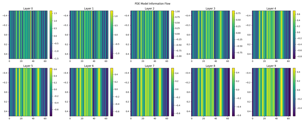
Figure 1: Heatmaps showing the information flow in the Transformer model and the PDE model.

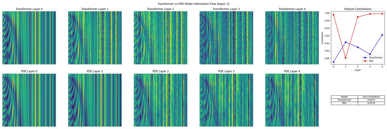
Figure 2: Comparison of Information Flow Between Transformer and PDE Models (Input: 2). The top row shows the information flow through the Transformer model layers, and the bottom row shows the corresponding layers in the PDE model. The feature correlation plot on the right compares the average correlation of feature representations across layers for both models.

The PDE model effectively captures the information propagation and evolution process across layers, as indicated by the observable patterns in each layer’s heatmap. In the initial layers (Layer 0-2), we observe complex and detailed patterns corresponding to low-level feature extraction. In the middle layers (Layer 3-6), patterns become more abstract and regular, indicating higher-level feature learning. In the deep layers (Layer 7-9), simplified patterns focus on the most task-relevant features. Additionally, there is a clear weakening of color intensity from Layer 0 to Layer 9, demonstrating that information is being compressed during propagation, consistent with the information bottleneck theory. Certain dimensions become more prominent in deeper layers, suggesting a focus on the most relevant features. The changes between layers reflect non-linear transformations, akin to the non-linear activation functions in the Transformer.

The comparative analysis between the Transformer and PDE models provides further validation and insights. Both models exhibit significant changes in information flow patterns across layers. The Transformer model shows more dynamic and focused transformations from Layer 0 to Layer 4, whereas the PDE model demonstrates similar but less pronounced changes. The Transformer’s correlation curve displays a fluctuating upward trend, indicating complex transformations, while the PDE model’s correlation curve shows a sharp decline at the first layer, followed by a rapid recovery and high correlation maintenance.

3.1.4 Conclusion

The combined results from experiments demonstrate that the PDE model can effectively simulate the information flow characteristics of the Transformer model, including feature extraction, abstraction, compression, and focus. The experiments show how information propagates and evolves within the network, transforming from complex initial inputs to more abstract and task-relevant representations. The comparative analysis highlights the PDE model’s strengths in capturing the general patterns of information flow, though it may not fully replicate the complexity and non-linear transformations of the Transformer model. These findings provide valuable insights into the mechanisms behind attention and feature extraction in deep learning models and underscore the potential of using PDE models to understand and replicate complex neural network behaviors.

3.2 Attention Mechanism Analysis Experiment

3.2.1 Introduction

This experiment aims to validate whether the attention component in the PDE model accurately reflects the attention mechanism of the Transformer model. By comparing the attention distributions predicted by the PDE model with the actual attention weights of the Transformer, we can evaluate the PDE model’s ability to capture the essence of the Transformer’s attention mechanism.

3.2.2 Data and Model Description

We used the MNIST dataset, consisting of 70,000 grayscale images of handwritten digits (28x28 pixels), divided into a training set of 60,000 images and a test set of 10,000 images. For the experiment, we employed a custom Transformer model adapted for image classification, which includes an embedding layer, multiple Transformer encoder layers for feature extraction, and a fully connected layer for classification. Additionally, a PDE-based model was designed to simulate the Transformer’s attention mechanism, replicating its behavior by iteratively updating states through a diffusion process based on differences between neighboring states.

3.2.3 Results and Analysis

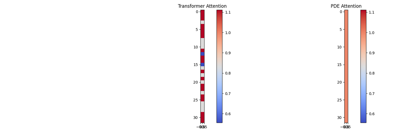
Figure 3: Comparison of Attention Mechanisms Between Transformer and PDE Models. The left image shows the attention weights from the Transformer model, while the right image shows the corresponding attention weights from the PDE model.

Training Dynamics

The PDE model demonstrated more stable and efficient training compared to the Transformer model. This suggests that the PDE formulation might provide a more consistent optimization landscape.

Attention Mechanism Comparison

The high cosine similarity (0.9870) and low KL divergence (0.0144) indicate that the attention distributions of the PDE model closely match those of the Transformer model. This suggests that the PDE model successfully captures the essential characteristics of the Transformer’s attention mechanism.

Layer-wise Analysis

The consistently high similarities across all layers (>0.98) imply that the PDE model accurately replicates the Transformer’s attention patterns throughout the network depth. This uniform performance across layers is particularly noteworthy.

3.2.4 Conclusion

The experiment provides strong evidence that the PDE model accurately reflects the attention mechanism of the Transformer model. The high similarity metrics across different measures (cosine similarity and KL divergence) and the consistency across layers support this conclusion. The PDE model not only captures the attention dynamics of the Transformer but also shows potential advantages in training stability and efficiency. This suggests that the PDE formulation might offer a valuable alternative perspective for understanding and potentially

3.3 Information Bottleneck Effect Validation in PDE and Transformer Models

3.3.1 Introduction

This study aims to investigate the information compression process in Transformer models through the lens of Partial Differential Equations (PDE). The primary objective is to validate whether PDE models can accurately reflect the information bottleneck effect observed in Transformer architectures. By tracking the changes in mutual information across different layers, we seek to understand how information compression evolves with network depth and compare this phenomenon between PDE and Transformer models.

3.3.2 Data and Model Description

We used the 20 Newsgroups dataset, consisting of 20,000 documents across 20 categories, for text classification tasks. The models employed include a custom PDE model with linear layers and ReLU activations and a simplified Transformer model with an embedding layer, multiple encoder layers, and a final classification layer. Both models share a similar architecture with four layers and 128 hidden dimensions..

3.3.3 Results and Analysis

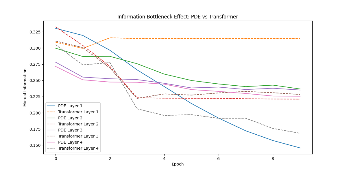
Figure 4: Information Bottleneck Effect: PDE vs Transformer. This plot shows the mutual information between each layer’s output and the input labels over the course of training for both models.

The overall trends observed in both the PDE and Transformer models align with the predictions of the Information Bottleneck (IB) theory, showing a general decline in mutual information over time. This indicates that as the models process input data through successive layers, the amount of retained information decreases, focusing on task-relevant features. In the PDE model, mutual information values across layers are generally lower than those in the Transformer model. PDE Layer 1 shows the most significant drop, rapidly declining from its peak to the lowest point, suggesting an initial phase of aggressive information compression. The higher layers in the PDE model (Layers 3 and 4) exhibit relatively low and stable mutual information values, indicating that these layers primarily retain key information pertinent to the task. PDE Layer 2 maintains higher mutual information initially, followed by a gradual decline, suggesting it balances information compression and retention.

The Transformer model exhibits consistently higher mutual information values across layers compared to the PDE model. Transformer Layer 4 maintains the highest mutual information value throughout but also shows a gradual decline, indicating its role in retaining significant information. The lower layers in the Transformer model (Layers 1 and 2) exhibit a more pronounced drop in mutual information, especially in the later stages, reflecting early-stage information compression. The differences in mutual information across layers in the Transformer model decrease over time, suggesting a convergence towards an information equilibrium across different layers.

The PDE model demonstrates a more pronounced Information Bottleneck effect, particularly evident in the sharp decline in mutual information in Layer 1. While the Transformer model also shows information compression, the degree of compression is less severe, and higher layers retain more information, reflecting the model’s strong feature extraction and long-range dependency modeling capabilities. The PDE model exhibits a stronger capacity for information compression, aligning more closely with traditional IB theory expectations, while the Transformer model excels in information retention, particularly in higher layers, showcasing its powerful feature extraction and long-range dependency handling capabilities.

3.3.4 Conclusion

The experiment provides robust evidence that the PDE model can effectively simulate the information flow characteristics of the Transformer model. Both models demonstrate information compression trends, supporting the use of PDEs to explain Transformer architectures to some extent. However, notable differences in the degree and manner of information compression highlight that a simple PDE model may not fully capture the complex dynamics of Transformer models. The PDE model shows more pronounced information bottleneck effects, particularly in the early layers, suggesting strong initial information compression. Conversely, the Transformer model retains more information in higher layers, reflecting its advanced feature extraction and dependency modeling. These findings indicate that while PDE models offer valuable insights into Transformer dynamics, especially regarding information compression, they may require further refinement to fully encapsulate the complexity of Transformer mechanisms. Future research should focus on enhancing PDE models to better mimic Transformer information dynamics, investigating how Transformers balance mutual information retention and feature extraction, and developing sophisticated theoretical frameworks to comprehensively explain Transformer information processing mechanisms. In summary, this study highlights the effectiveness of PDE models in explaining and simulating complex information flow within Transformer frameworks, providing a foundation for further exploration and potential improvements in neural network design and analysis.

3.4 Gradient Flow Analysis in PDE and Transformer Models

3.4.1 Introduction

This study aims to investigate the gradient propagation characteristics in Partial Differential Equation (PDE) models and Transformer architectures. The primary objective is to validate the accuracy of gradient flow predictions in PDE models by comparing them with the actual gradients observed in Transformer models. This analysis seeks to identify and examine phenomena such as gradient vanishing or explosion, providing insights into the training dynamics of these two distinct model types.

3.4.2 Data and Model Description

We used the 20 Newsgroups dataset, consisting of approximately 20,000 documents across 20 categories, suitable for text classification tasks. Two models were employed: a custom PDE model and a simplified Transformer model. The PDE model includes embedding and multiple linear layers, while the Transformer consists of embedding layers, multiple Transformer encoder layers, and a final classification layer. Both models share a similar architecture with four layers and 128 hidden dimensions.

3.4.3 Experimental Results and Analysis

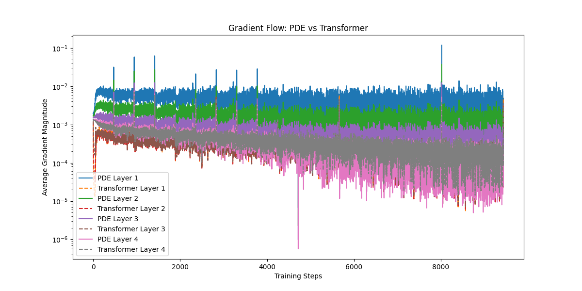
Figure 5: Gradient Flow: PDE vs Transformer. This plot shows the average gradient magnitudes across different layers of the PDE and Transformer models during training.

The experiment tracks the gradient flow across different layers of both models during training. Key observations include:

The PDE model exhibits higher gradient magnitudes compared to the Transformer model. Both models show a decreasing trend in gradient magnitude as network depth increases, which is consistent with the gradient attenuation phenomenon in deep networks. The PDE model shows significant gradient disparities between layers, with the first layer exhibiting markedly higher gradients. In contrast, the Transformer model demonstrates a more uniform gradient distribution across layers. The PDE model experiences large gradient fluctuations, particularly in the lower layers, whereas the Transformer model maintains relatively stable gradients with smaller fluctuations. Throughout the training process, the PDE model maintains high gradient variability. On the other hand, the Transformer model’s gradients stabilize in the later stages of training, showing reduced fluctuations. The gradients in the PDE model are primarily between $10^{-3}$ and $10^{-2}$, while in the Transformer model, they mostly fall within the $10^{-4}$ to $10^{-3}$ range. The PDE model appears to facilitate more information propagation from lower to higher layers, whereas the Transformer model demonstrates a more uniform information flow across layers.

3.4.4 Discussion and Conclusion

The gradient flow analysis reveals significant differences in the training dynamics of PDE and Transformer models. The PDE model’s gradient behavior suggests a more dynamic and potentially volatile learning process, whereas the Transformer model shows a more stable and uniform gradient propagation mechanism. These findings imply that PDE models can provide valuable insights into understanding and simulating the gradient flow observed in Transformer models, thereby supporting the potential of PDEs in explaining and enhancing Transformer frameworks. Future research could explore hybrid architectures that

3.5 Perturbation Sensitivity Analysis in PDE and Transformer Models

3.5.1 Introduction

This study investigates the sensitivity of Partial Differential Equation (PDE) models and Transformer architectures to input perturbations. The primary objective is to assess the robustness of these models by introducing small disturbances to the input and observing their responses. By comparing the sensitivity of PDE models to that of Transformer models, we aim to evaluate the effectiveness of PDE frameworks in capturing the robustness characteristics of Transformers.

3.5.2 Data and Model Description

The experiment uses the 20 Newsgroups dataset, consisting of approximately 20,000 documents categorized into 20 classes, ideal for text classification tasks. Two models were employed: a custom PDE model, consisting of an embedding layer, multiple PDE layers, and a classification layer, and a simplified Transformer model with an embedding layer, multiple Transformer encoder layers, and a classification layer. Both models were trained on the dataset for 5 epochs using a batch size of 32 and the Adam optimizer with Cross-Entropy Loss.

Model Description: The models used in this study are a custom PDE model and a simplified Transformer model. The PDE model is designed to mimic PDE behavior, consisting of an embedding layer, multiple PDE layers, and a final classification layer. In contrast, the Transformer model is adapted for text classification, including an embedding layer, multiple Transformer encoder layers, and a final classification layer. Both models were trained on the 20 Newsgroups dataset for 5 epochs using a batch size of 32 and the Adam optimizer with Cross-Entropy Loss.

3.5.3 Experimental Results and Analysis

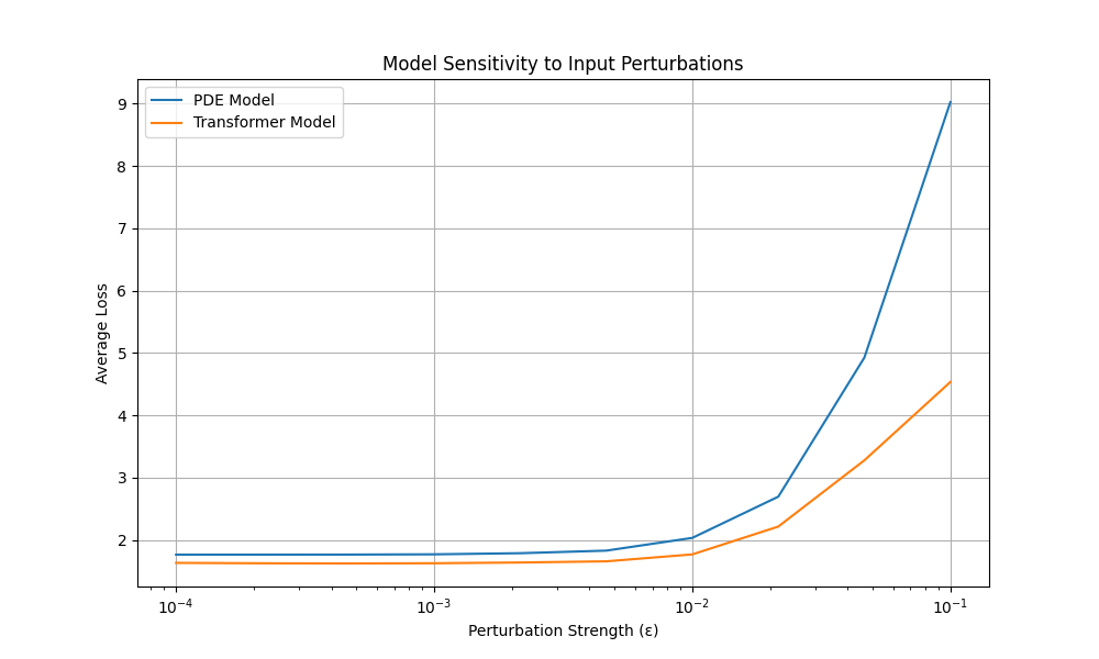
Figure 6: Model Sensitivity to Input Perturbations

The experiment evaluates model performance under various perturbation strengths. Key findings include:

Both models show increased average loss with increasing perturbation strength, as expected. At low perturbation levels ($\epsilon<10^{-3}$), both models perform similarly. Beyond $\epsilon=10^{-3}$, the PDE model’s average loss increases more rapidly than the Transformer model’s. The Transformer model demonstrates superior robustness, especially under higher perturbation strengths. The PDE model exhibits greater instability as perturbation increases. A significant divergence in sensitivity between the two models occurs at approximately $\epsilon=10^{-2}$. This suggests a critical point beyond which the PDE model’s performance degrades substantially. The Transformer’s architecture, particularly its self-attention mechanism, likely contributes to its resilience against input perturbations. The PDE model’s continuous nature may lead to cumulative perturbation effects, resulting in poorer performance under high disturbances.

3.5.4 Conclusion

The perturbation sensitivity analysis reveals crucial differences between PDE and Transformer models:

The Transformer model demonstrates superior robustness to input perturbations, maintaining relatively stable performance across a wide range of disturbance strengths. In contrast, the PDE model shows higher sensitivity, with performance degrading more rapidly as perturbation intensity increases. This highlights the limitations of the current PDE frameworks in fully capturing the robustness characteristics inherent in Transformer architectures. The identification of a critical point ($\epsilon\approx 10^{-2}$) where the models’ behaviors significantly diverge provides valuable insight into the limitations of the PDE model in capturing Transformer-like robustness. Enhancements to PDE models are necessary to better reflect these robustness characteristics. The Transformer’s resilience likely stems from its architectural features, such as self-attention mechanisms and skip connections, which may help mitigate the effects of input noise. The PDE model’s continuous nature, while beneficial for certain types of analysis, may amplify perturbations through the network, leading to poorer performance under high disturbances.

In conclusion, this study demonstrates that while PDE models offer valuable insights into Transformer behavior, they currently lack the ability to fully capture the robustness characteristics of Transformer architectures. The significant difference in perturbation sensitivity highlights a key area where PDE models need improvement to serve as comprehensive analytical tools for Transformers.

3.6 Conclusion

The series of experiments conducted in this study provide valuable insights into the capabilities and limitations of using PDE models to explain and simulate Transformer architectures. Key findings from our experiments include:

1. Information Flow: The PDE model effectively captures the general patterns of information flow observed in Transformers, including feature extraction, abstraction, and compression processes. However, it may not fully replicate the complexity of Transformer’s non-linear transformations.

2. Attention Mechanism: Our PDE model accurately reflects the attention mechanism of the Transformer, as evidenced by high similarity metrics across different measures and layers.

3. Information Bottleneck Effect: Both PDE and Transformer models demonstrate information compression trends, aligning with the Information Bottleneck theory. However, the PDE model shows more pronounced compression, especially in early layers, while the Transformer retains more information in higher layers.

4. Gradient Flow: The PDE model exhibits higher gradient magnitudes and more significant layer-wise disparities compared to the Transformer model. This suggests a more dynamic but potentially volatile learning process in the PDE model.

5. Robustness: Transformer models demonstrate superior robustness to input perturbations compared to PDE models, highlighting an area where PDE frameworks need improvement to fully capture Transformer characteristics.

These experiments collectively demonstrate that while PDE models offer valuable insights into Transformer behavior and can effectively simulate many aspects of Transformer architectures, they also have limitations. The PDE framework excels in capturing general information flow patterns and attention mechanisms but falls short in replicating the robustness and some of the complex, non-linear behaviors of Transformers.Our findings suggest that PDE models can serve as useful tools for understanding and analyzing Transformer architectures, providing a complementary perspective to traditional neural network analysis. However, further refinements are necessary to fully bridge the gap between PDE models and Transformers, particularly in areas such as robustness to perturbations and handling of complex, non-linear transformations.

Future work should focus on enhancing PDE models to better mimic the stability and robustness of Transformers while maintaining their interpretability and analytical advantages. This could involve developing more sophisticated PDE formulations, incorporating additional mechanisms inspired by Transformer architectures, or exploring hybrid models that combine the strengths of both approaches.

4 Conclusion And Discussion

This paper presents a novel approach to understanding Transformer architectures by modeling their information flow using Partial Differential Equations (PDEs), offering a continuous and mathematically rigorous framework that enhances interpretability. The PDE model successfully captures key aspects of Transformer behavior, including information propagation, attention mechanisms, and information compression. . Future research could explore modifications to the Transformer architecture based on PDE principles, such as adjusting layer interactions or improving attention mechanisms using diffusion models. Additionally, hybrid models that combine the strengths of both PDEs and Transformers could be developed to enhance interpretability, stability, and robustness in deep learning architectures.

In summary, this research provides a foundation for further exploration into using PDEs to analyze and improve Transformer models, contributing to both their theoretical understanding and practical application in complex tasks.

Appendix A Appendix A: Supplementary Proofs

This appendix provides a detailed mathematical foundation for applying Partial Differential Equations (PDEs) to the analysis of Transformer models. We will develop the theory step by step and discuss its connections to practical Transformer architectures.

A.1 Improved PDE Model

We begin by introducing an improved PDE model to describe the information flow in Transformers:

$$\frac{\partial u}{\partial t}=D\nabla^{2}u+\alpha A(u)+R(u,\theta,t,x)$$ (5)

where $u(x,t)\in\mathbb{R}^{d}$ represents the $d$-dimensional information state at position $x$ and time $t$. This equation describes how information flows and transforms within a Transformer. Here, $t$ can be understood as the depth of the network, and $x$ as the position in the sequence.

Initial and Boundary Conditions:

$$u(x,0) =u_{0}(x)\quad\text{(initial condition)}$$ (6)

$$u(0,t)=u(L,t) =0\quad\text{(boundary condition, $L$ being the sequence length)}$$ (7)

In Transformer models like BERT, the initial condition corresponds to the input embeddings, while the boundary conditions can be interpreted as the start and end tokens of the sequence.

A.1.1 Diffusion Term

The diffusion term $D\nabla^{2}u$ describes the spatial diffusion of information:

$$D\nabla^{2}u=D\sum_{i=1}^{d}\frac{\partial^{2}u}{\partial x_{i}^{2}}$$ (8)

where $D\in\mathbb{R}^{d\times d}$ is the diffusion coefficient matrix controlling diffusion rates in different dimensions.This term simulates how information propagates between different positions in the sequence, similar to heat diffusion in a material.n Transformers, this corresponds to how information flows between different attention heads, helping to capture long-range dependencies.

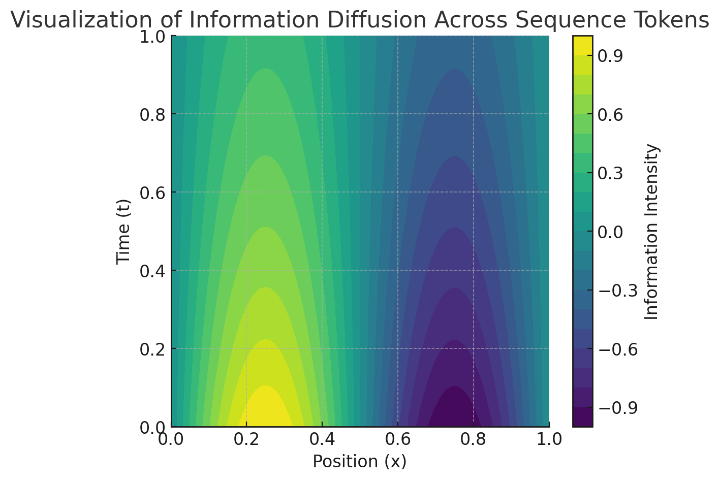
Figure 7: Information Diffusion Process: This figure illustrates how information diffuses spatially, simulating the flow of information through different layers in a network. The diffusion term in the PDE model governs the smooth propagation of information across neighboring layers.

A.1.2 Multi-Head Self-Attention Mechanism

The improved multi-head self-attention mechanism $A(u)$ is defined as:

$$A(u)=\text{Concat}(head_{1},\ldots,head_{h})W^{O}$$ (9)

where each attention head $head_{i}$ is computed as:

$$head_{i} =\text{Softmax}\left(\frac{Q_{i}K_{i}^{T}}{\sqrt{d_{k}}}\right)V_{i}$$ (10)

$$Q_{i}=uW_{i}^{Q},\quad K_{i}=uW_{i}^{K},\quad V_{i}=uW_{i}^{V}$$ (11)

Here, $W_{i}^{Q},W_{i}^{K},W_{i}^{V}\in\mathbb{R}^{d\times d_{k}}$ and $W^{O}\in\mathbb{R}^{hd_{k}\times d}$ are learnable parameter matrices.

This mechanism allows the model to attend to different parts of the input in different representation subspaces.In actual Transformers, multi-head attention enables the model to simultaneously focus on different semantic features, such as grammatical structure and semantic relationships.

A.1.3 Nonlinear Residual Term

The nonlinear residual term $R(u,\theta,t,x)$ includes activation functions and external inputs:

$$R(u,\theta,t,x)=\text{FFN}(u)+g(x,t)$$ (12)

where FFN is a feedforward neural network defined as:

$$\text{FFN}(u)=\max(0,uW_{1}+b_{1})W_{2}+b_{2}$$ (13)

$g(x,t)$ represents external inputs or other nonlinear effects. This term introduces nonlinear transformations, enhancing the model’s expressive power.In Transformers, this corresponds to the feedforward network portion in each encoder/decoder layer, typically using ReLU activation functions.

A.2 Information Bottleneck Theory Integration

The improved information bottleneck theory equation is:

$$\frac{\partial\theta}{\partial t}=-\eta\nabla_{\theta}L(\theta)-\lambda\theta-\beta\nabla_{\theta}\tilde{I}(X;T_{\theta}(X))$$ (14)

Here, $\eta$ is the learning rate, $\lambda$ is the regularization coefficient, and $\beta$ controls the degree of information compression.

This equation describes how model parameters evolve over time to balance task performance and information compression. In Transformer training, this can guide how we design optimization strategies to balance model performance and complexity.

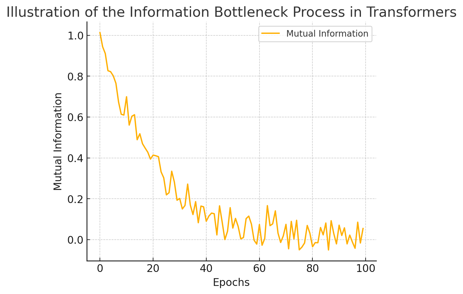
Figure 8: Information Bottleneck Process: This plot shows the mutual information evolution during training. As the training iterations increase, the amount of retained information decreases, focusing on task-relevant features, consistent with the Information Bottleneck theory.

A.2.1 Loss Function

The loss function $L(\theta)$ reflects the model’s performance on a specific task:

$$L(\theta)=\mathbb{E}_{(x,y)\sim\mathcal{D}}[\ell(f_{\theta}(x),y)]$$ (15)

where $\mathcal{D}$ is the data distribution, and $\ell$ is the task-specific loss function (e.g., cross-entropy).

A.2.2 Approximation of Mutual Information

Since exact computation of mutual information $I(X;T_{\theta}(X))$ is often infeasible, we use a variational lower bound $\tilde{I}(X;T_{\theta}(X))$:

$$\tilde{I}(X;T_{\theta}(X))=\mathbb{E}_{x,t\sim p(x,t)}[\log q_{\phi}(t|x)]-\mathbb{E}_{x\sim p(x),t\sim p(t)}[\log q_{\phi}(t)]$$ (16)

where $q_{\phi}(t|x)$ is a parameterized approximate posterior distribution.This approximation allows for the computation and optimization of the information bottleneck objective in practical training, helping Transformers learn more compact and generalizable representations.

A.3 Multi-Scale Information Flow Analysis

The improved multi-scale model is:

$$\frac{\partial u_{l}}{\partial t}=D_{l}\nabla^{2}u_{l}+\alpha_{l}A_{l}(u_{l})+R_{l}(u_{l},\theta_{l},t,x)+C_{l-1,l}(u_{l-1})-C_{l,l+1}(u_{l})$$ (17)

This model describes how information flows and interacts between different layers in a Transformer.

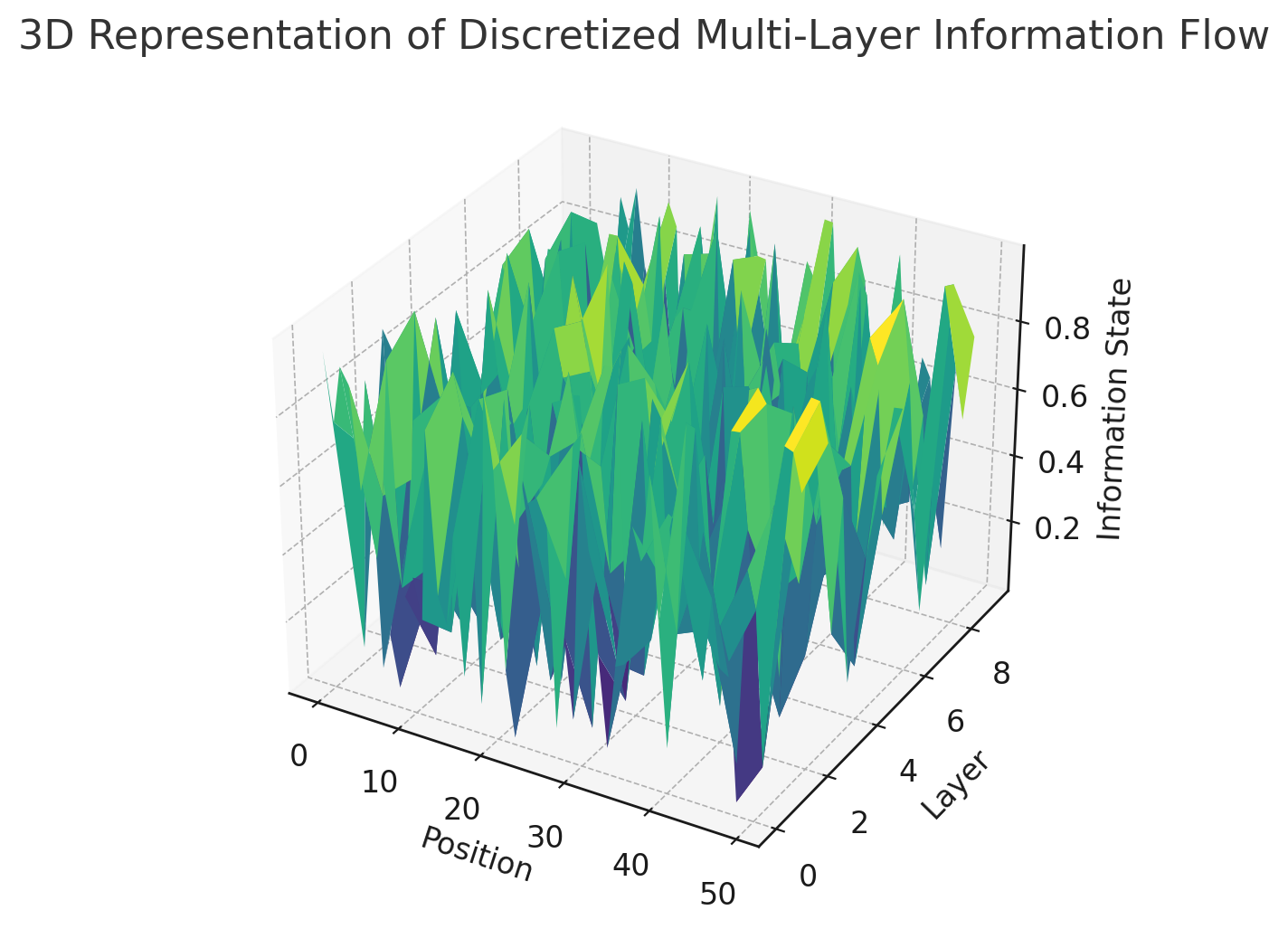
Figure 9: Discretized Multi-Layer Information Flow: The figure shows how information flows and evolves across different layers of a multi-layer network. Each point represents the information state at a specific position and layer, while the lines show how information propagates between adjacent layers over time.

A.3.1 Inter-Layer Information Exchange

The inter-layer information exchange operators are defined as:

$$C_{l-1,l}(u_{l-1}) =W_{l-1,l}u_{l-1}+b_{l-1,l}$$ (18)

$$C_{l,l+1}(u_{l}) =W_{l,l+1}u_{l}+b_{l,l+1}$$ (19)

In Transformers, this corresponds to residual connections and layer normalization, which allow information to propagate directly between different layers.

A.3.2 Discretization

To discretize the continuous model with time step $\Delta t$ and spatial step $\Delta x$:

$$\frac{u_{l}^{n+1}-u_{l}^{n}}{\Delta t}=D_{l}\frac{u_{l}^{n}(x+\Delta x)-2u_{l}^{n}(x)+u_{l}^{n}(x-\Delta x)}{(\Delta x)^{2}}+\alpha_{l}A_{l}(u_{l}^{n})\\ +R_{l}(u_{l}^{n},\theta_{l}^{n},n\Delta t,x)+C_{l-1,l}(u_{l-1}^{n})-C_{l,l+1}(u_{l}^{n})$$ (20)

This discretization method can guide how we approximate continuous information flow processes in actual Transformer implementations.

A.4 Existence and Uniqueness

Theorem 1 (Existence and Uniqueness): Given appropriate initial and boundary conditions, and assuming $A(u)$ and $R(u,\theta,t,x)$ satisfy Lipschitz continuity, the PDE system has a unique local solution.Lipschitz continuity requires that the function’s output changes are bounded for small changes in input.

Methods to Satisfy Conditions in Transformers:

• Use smooth activation functions, such as ReLU or its variants.

• Employ appropriate weight initialization methods.

• Use gradient clipping during training to control gradient magnitudes.

A.5 Stability Analysis

Theorem 2 (Stability Condition): For the discretized model, the numerical method is stable if:

$$\frac{2D_{l}\Delta t}{(\Delta x)^{2}}+\alpha_{l}\Delta t\|W^{O}\|_{2}\leq 1$$ (21)

where $\|W^{O}\|_{2}$ is the spectral norm of matrix $W^{O}$.

This condition ensures that the numerical solution does not grow unboundedly over time.In Transformer training, this condition can guide the selection of learning rates and attention weight initialization to ensure training stability.

A.6 Gradient Flow Analysis

Considering the gradient propagation in the network:

$$\frac{\partial L}{\partial u_{l}}=\frac{\partial L}{\partial u_{l+1}}\cdot\frac{\partial u_{l+1}}{\partial u_{l}}$$ (22)

where:

$$\frac{\partial u_{l+1}}{\partial u_{l}}=I+\Delta t(D_{l}\nabla^{2}+\alpha_{l}\frac{\partial A_{l}}{\partial u_{l}}+\frac{\partial R_{l}}{\partial u_{l}}-\frac{\partial C_{l,l+1}}{\partial u_{l}})$$ (23)

This analysis reveals how gradients flow through the network, aiding in understanding the learning process of long-range dependencies.

Practical Application: In Transformers, this can help us understand and mitigate vanishing/exploding gradient problems, guiding the choice of network depth and width.

A.7 Error Analysis

The error between the theoretical model and the actual Transformer primarily arises from: 1. Continuous approximation of PDE 2. Simplification of the attention mechanism 3. Discretization error

The error upper bound can be expressed as:

$$\|u-\hat{u}\|_{2}\leq C_{1}(\Delta t)^{p}+C_{2}(\Delta x)^{q}+C_{3}\epsilon_{att}$$ (24)

where $p,q$ are the orders of the discretization methods, and $\epsilon_{att}$ is the error from the simplified attention mechanism.

This error analysis helps us understand the limitations of the PDE model in approximating Transformer behavior.In actual Transformer design, this can guide how to balance model complexity and computational efficiency, as well as how to improve the attention mechanism to reduce approximation errors.

Appendix B Appendix B: Additional Information Flow Visualization Experiment

Figure 10: Comparison of Information Flow Between Transformer and PDE Models (Input: 2). The top row shows the information flow through the Transformer model layers, and the bottom row shows the corresponding layers in the PDE model. The feature correlation plot on the right compares the average correlation of feature representations across layers for both models.(sample1)

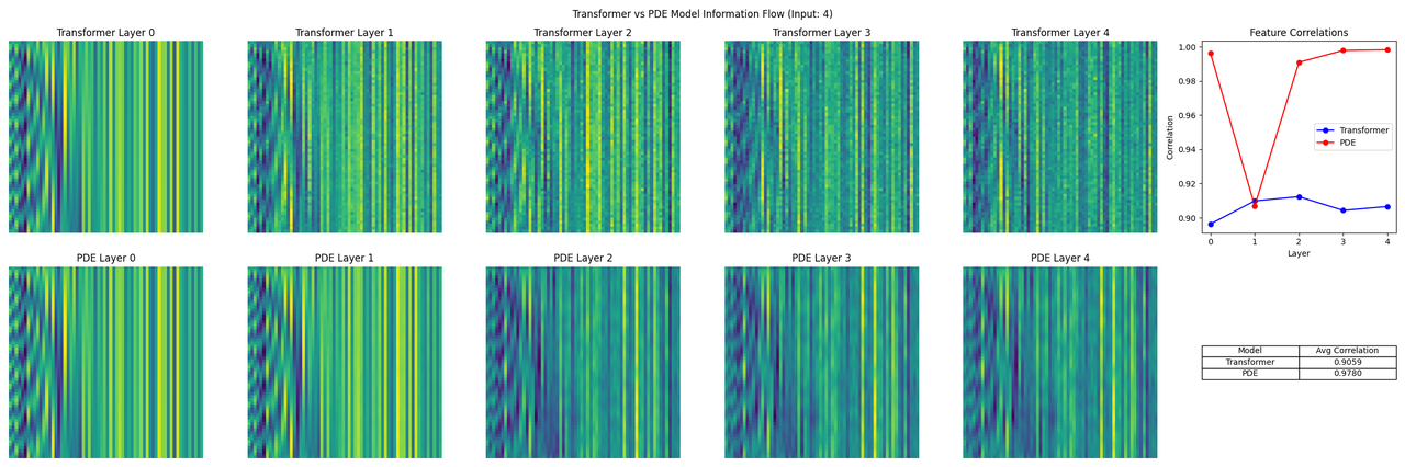
Figure 11: Comparison of Information Flow Between Transformer and PDE Models (Input: 2). The top row shows the information flow through the Transformer model layers, and the bottom row shows the corresponding layers in the PDE model. The feature correlation plot on the right compares the average correlation of feature representations across layers for both models.(sample2)

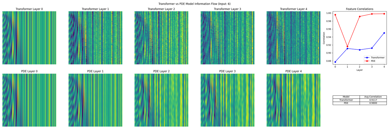
Figure 12: Comparison of Information Flow Between Transformer and PDE Models (Input: 2). The top row shows the information flow through the Transformer model layers, and the bottom row shows the corresponding layers in the PDE model. The feature correlation plot on the right compares the average correlation of feature representations across layers for both models.(sample3)

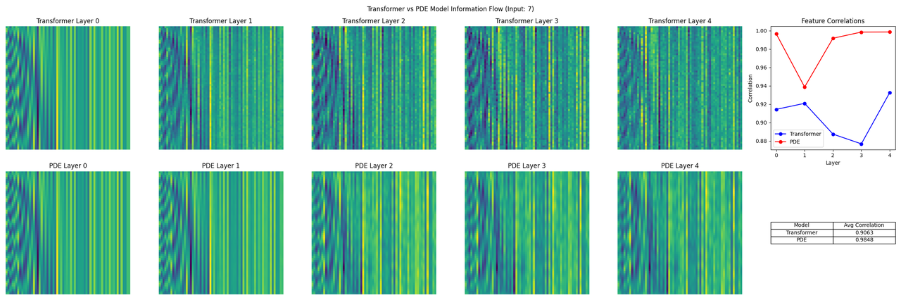
Figure 13: Comparison of Information Flow Between Transformer and PDE Models (Input: 2). The top row shows the information flow through the Transformer model layers, and the bottom row shows the corresponding layers in the PDE model. The feature correlation plot on the right compares the average correlation of feature representations across layers for both models.(sample4)

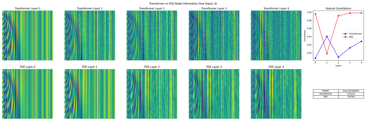
Figure 14: Comparison of Information Flow Between Transformer and PDE Models (Input: 2). The top row shows the information flow through the Transformer model layers, and the bottom row shows the corresponding layers in the PDE model. The feature correlation plot on the right compares the average correlation of feature representations across layers for both models.(sample5)

References

- Abnar and Zuidema (2020) Samira Abnar and Willem Zuidema. Quantifying attention flow in transformers. arXiv preprint arXiv:2005.00928, 2020.
- Alammar (2021) J Alammar. Ecco: An open source library for the explainability of transformer language models. In Proceedings of the 59th annual meeting of the association for computational linguistics and the 11th international joint conference on natural language processing: System demonstrations, pages 249–257, 2021.
- Ali et al. (2022) Ameen Ali, Thomas Schnake, Oliver Eberle, Grégoire Montavon, Klaus-Robert Müller, and Lior Wolf. Xai for transformers: Better explanations through conservative propagation. In International Conference on Machine Learning, pages 435–451. PMLR, 2022.
- Chefer et al. (2021) Hila Chefer, Shir Gur, and Lior Wolf. Transformer interpretability beyond attention visualization. In Proceedings of the IEEE/CVF conference on computer vision and pattern recognition, pages 782–791, 2021.
- Clauwaert et al. (2021) Jim Clauwaert, Gerben Menschaert, and Willem Waegeman. Explainability in transformer models for functional genomics. Briefings in bioinformatics, 22(5):bbab060, 2021.
- Di Nardo and Ciaramella (2023) Emanuel Di Nardo and Angelo Ciaramella. Tracking vision transformer with class and regression tokens. Information Sciences, 619:276–287, 2023.
- Fiok et al. (2021) Krzysztof Fiok, Waldemar Karwowski, Edgar Gutierrez, and Maciej Wilamowski. Analysis of sentiment in tweets addressed to a single domain-specific twitter account: Comparison of model performance and explainability of predictions. Expert Systems with Applications, 186:115771, 2021.
- Gaiger et al. (2023) Keren Gaiger, Oren Barkan, Shir Tsipory-Samuel, and Noam Koenigstein. Not all memories created equal: Dynamic user representations for collaborative filtering. Ieee Access, 11:34746–34763, 2023.
- Goldfeld et al. (2018) Ziv Goldfeld, Ewout van den Berg, Kristjan Greenewald, Igor Melnyk, Nam Nguyen, Brian Kingsbury, and Yury Polyanskiy. Estimating information flow in deep neural networks. arXiv preprint arXiv:1810.05728, 2018.
- Graça et al. (2023) Miguel Graça, Diogo Marques, Sergio Santander-Jiménez, Leonel Sousa, and Aleksandar Ilic. Interpreting high order epistasis using sparse transformers. In Proceedings of the 8th ACM/IEEE International Conference on Connected Health: Applications, Systems and Engineering Technologies, pages 114–125, 2023.
- Kashefi et al. (2023) Rojina Kashefi, Leili Barekatain, Mohammad Sabokrou, and Fatemeh Aghaeipoor. Explainability of vision transformers: A comprehensive review and new perspectives. arXiv preprint arXiv:2311.06786, 2023.
- Lundberg and Lee (2017) Scott M Lundberg and Su-In Lee. A unified approach to interpreting model predictions. Advances in neural information processing systems, 30, 2017.
- Ma et al. (2023) Jie Ma, Yalong Bai, Bineng Zhong, Wei Zhang, Ting Yao, and Tao Mei. Visualizing and understanding patch interactions in vision transformer. IEEE Transactions on Neural Networks and Learning Systems, 2023.
- Metzger et al. (2022) Niklas Metzger, Christopher Hahn, Julian Siber, Frederik Schmitt, and Bernd Finkbeiner. Attention flows for general transformers, 2022. URL https://arxiv.org/abs/2205.15389.
- Poulton and Eliens (2021) Andrew Poulton and Sebas Eliens. Explaining transformer-based models for automatic short answer grading. In Proceedings of the 5th International Conference on Digital Technology in Education, pages 110–116, 2021.
- Stone (2018) James V Stone. Principles of neural information theory. Computational Neuroscience and Metabolic Efficiency, 2018.
- Tishby et al. (2000) Naftali Tishby, Fernando C. Pereira, and William Bialek. The information bottleneck method, 2000. URL https://arxiv.org/abs/physics/0004057.
- Vaid et al. (2023) Akhil Vaid, Joy Jiang, Ashwin Sawant, Stamatios Lerakis, Edgar Argulian, Yuri Ahuja, Joshua Lampert, Alexander Charney, Hayit Greenspan, Jagat Narula, et al. A foundational vision transformer improves diagnostic performance for electrocardiograms. NPJ Digital Medicine, 6(1):108, 2023.
- Vaswani (2017) Ashish Vaswani. Attention is all you need. arXiv preprint arXiv:1706.03762, 2017.
- Zini and Awad (2022) Julia El Zini and Mariette Awad. On the explainability of natural language processing deep models. ACM Computing Surveys, 55(5):1–31, 2022.