The Story Behind the Lines: Line Charts as a Gateway to Dataset Discovery

Abstract.

Line charts are a valuable tool for data analysis and exploration, distilling essential insights from a dataset. However, access to the underlying dataset behind a line chart is rarely readily available. In this paper, we explore a novel dataset discovery problem, dataset discovery via line charts, focusing on the use of line charts as queries to discover datasets within a large data repository that are capable of generating similar line charts. To solve this problem, we propose a novel approach called Fine-grained Cross-modal Relevance Learning Model (FCM), which aims to estimate the relevance between a line chart and a candidate dataset. To achieve this goal, FCM first employs a visual element extractor to extract informative visual elements, i.e., lines and y-ticks, from a line chart. Then, two novel segment-level encoders are adopted to learn representations for a line chart and a dataset, preserving fine-grained information, followed by a cross-modal matcher to match the learned representations in a fine-grained way. Furthermore, we extend FCM to support line chart queries generated based on data aggregation. Last, we propose a benchmark tailored for this problem since no such dataset exists. Extensive evaluation on the new benchmark verifies the effectiveness of our proposed method. Specifically, our proposed approach surpasses the best baseline by $30.1\%$ and $41.0\%$ in terms of prec@50 and ndcg@50, respectively.

1. Introduction

Dataset discovery involves the identification, assessment and selection of datasets from a large dataset repository based on specific requirements and objectives of a user (Brickley et al., 2019; Bogatu et al., 2020; Khatiwada et al., 2023; Fan et al., 2023). It has a pivotal role in data-driven workflows, and has a profound influence on the quality and success of subsequent data analyses. Depending on the user input, existing studies can be broadly divided into two categories: 1) keyword-based dataset discovery (Brickley et al., 2019), which aims to find datasets whose contents are the most relevant to a set of given keywords; 2) unionable or joinable dataset discovery (Bogatu et al., 2020; Khatiwada et al., 2023; Fan et al., 2023), which aims to find datasets (tables) that can be approximately joined or unioned with a user-provided table.

While keywords and tables serve as valuable inputs for dataset discovery, users may also seek alternative informative intermediaries. Line charts, which are common visual representations of data, have a pivotal role in effective communication and interpretation of information in data exploration and analysis tasks (Grant, 2018). In practice, users may be interested in the data patterns presented in a line chart and aim to identify the original datasets from which it was generated or find datasets with similar patterns. Therefore, in this work, we provide a new dimension of input for the dataset discovery problem, that is, given a line chart query, find top-$k$ relevant datasets that can generate line charts similar to the given one. This type of dataset discovery method not only serves as a starting point for open-ended data exploration by providing a collection of comprehensive datasets (Idreos et al., 2015), but it is also very user-friendly, as users can simply input the line chart of interest to obtain relevant datasets, bypassing the need for users to understand or write complex queries. Furthermore, given the widespread use of line charts to present data trends, this method is anticipated to have broad applications across numerous fields. For example, in journalism, this method helps in tracing original data sources from widely disseminated line charts, aiding in fact-checking (Graves and Amazeen, 2019). In clinical trials, it helps assist doctors in seeking relevant data for treatment decisions or participant recruitment, especially considering the frequent use of line charts like electrocardiograms in medical contexts (Cai et al., 2011). In consulting, consultants can identify relevant datasets corresponding to a given line chart, which is essential for thorough due diligence processes requiring detailed and comprehensive data (Cumming and Zambelli, 2017).

Our work draws inspirations from and contributes to two related research fields: databases and visualization. In the field of databases, it aligns with the well-established practice of dataset discovery (Bogatu et al., 2020; Khatiwada et al., 2023; Fan et al., 2023), as discussed earlier. In the field of visualization, it is similar to chart search (Li et al., 2022b; Masson et al., 2023; Luo et al., 2023), which identifies visually similar charts using an exemplar, and benefits other foundational tasks such as visualization recommendation (Luo et al., 2018; Zhou et al., 2021; Ji et al., 2023). The above related work primarily focus on identifying relationships or similarities using a single data modality (e.g., table-to-table and image-to-image) or between two closely related modalities (e.g., text-to-table). Our research is unique as it is centered on two distinct data modalities: structural tables and image data, providing a novel contribution to the exploration of relationships and similarities across disparate data modalities.

Specifically, the novelty of dataset discovery via line charts can be demonstrated as follows. First, we avoid imposing rigid constraints on the exemplar line chart input, requiring only two essential visual elements–namely, lines and the y-ticks. Additionally, the line chart can feature either a single line or multiple lines. More importantly, we extend our scope to encompass line charts depicting visual outcomes derived from data aggregation operations applied to a dataset. This extension is significant as data aggregation commonly serves as an operator to summarize data.

Compared to existing dataset discovery problems, our problem faces two unique challenges.

• Challenge 1: Cross-modal Relevance. Defining an appropriate relevance metric between an exemplar line chart and a candidate dataset significantly impacts the quality of discovered datasets. In this bimodal task, utilizing both image and tabular data, it deviates from the majority of existing dataset discovery methods (Bogatu et al., 2020; Santos et al., 2021; Khatiwada et al., 2023), which predominantly focus on a single modality.

• Challenge 2: Data Shift between Aggregated Data and Original Data. A line chart can be generated by aggregating data from the original dataset, introducing a shift gap between the aggregated and original data. This shift is further complicated by the multitude of valid data aggregation operators and the arbitrary aggregation window size. Therefore, to effectively address aggregation-based queries in our problem, it is essential to determine how to model data transformations created by various aggregation operators, capture the effects of different aggregation window sizes, and infer the most likely aggregation operator used for a given line chart.

To the best of our knowledge, this is the first work studying the problem of dataset discovery via line charts. Although two bodies of related work can be leveraged to tackle this problem, each has its limitations: 1) A combination of visualization recommendation (VisRec) (Luo et al., 2018) and chart search methods. VisRec methods can initially recommend suitable line charts for a candidate dataset, while chart search, a commonly used technique for identifying relevant charts, can rank the generated line charts. However, the performance is limited by the capabilities of the VisRec methods, and information loss may occur during the chart search process. 2) Time series search methods (Mannino and Abouzied, 2018b) enable users to find time series data for a given line sketch, but these methods struggle with multiple lines and data aggregation scenarios. In Section 7, we instantiate these two bodies of related work and demonstrate their limitations.

Our Contributions.

A Novel Cross-Modal Relevance Learning Model. To address the challenge of cross-modal relevance, we propose a novel model called Fine-grained Cross-modal Relevance Learning Model (FCM). FCM first employs a visual element extractor to extract essential visual elements, such as lines and y-tick values, from a line chart, which serve as key indicators of desirable datasets. Then, to match a dataset and a line chart, we propose two novel segment-level encoders to learn the representations of the line chart and the candidate dataset, preserving locality-based characteristics. Finally, a cross-modal matcher is created to match them in a fine-grained manner.

Handling Aggregation-based Queries. To address the challenge of data shift between the original data and the aggregated data, we enhance FCM with three innovative components in the dataset encoder: (1) The transformation layer aims to learn non-linear transformations produced by data aggregation operations. (2) The hierarchical multi-scale representation layer utilizes a tree structure to learn a comprehensive dataset representation that integrates information across various data segment sizes, corresponding to different window sizes. (3) The Mixture-of-Experts (Yuksel et al., 2012) layer learns the distribution about different aggregation operators in order to automatically infer the most likely aggregation operation used in a line chart.

Efficiency. We improve the efficiency of online query processing. Specifically, we propose a hybrid indexing strategy based on the interval tree (Kriegel et al., 2000) and locality sensitive hashing (Lv et al., 2007) to identify a small set of candidate datasets, which greatly reduces the number of relevance estimations required. (Sec. 6)

Benchmarks and Evaluation. As the first to explore dataset discovery via line charts, we establish a benchmark for evaluation based on Plotly (Hu et al., 2019). This benchmark will be publicly released after the paper is accepted. Extensive experiments demonstrate the effectiveness of our solution. When compared against the best baseline, the relative improvement of FCM is 30.1% and 41.0% in terms of prec@50 and ndcg@50, respectively. We also implement a system prototype in (Ji et al., 2024). (Sec. 7)

2. Problem Formulation

We first describe key concepts used in this work, and then introduce the problem of dataset discovery via line charts and how we transform it into a problem of cross-modal relevance learning.

Dataset. In this work, we consider a dataset to be a table of $N_{C}$ columns, namely $T=\{C_{1},C_{2},...,C_{N_{C}}\}$. Each column $C_{i}$ is expressed as a data series $C_{i}=(a_{1},a_{2},...,a_{N_{R}})$, where $N_{R}$ is the number of rows in $T$. Henceforth, we use “table” and “dataset” interchangeably.

Line Chart. A line chart $V$, employed as a visual representation, is a 2-D image presenting one or multiple data series across a continuous interval or time period. $V$ consists of several visual elements, out of which two are essential in every line chart:

• Lines are the key visual elements in a line chart that demonstrate how the underlying data will change within a given period. We introduce the concept of “underlying data” later in this section. A line chart may contain $M$ lines, denoted as $L=\{l_{1},l_{2},...,l_{M}\}$.

• Ticks are the markings or values displayed along each axis, indicating the range corresponding to the points of each line.

Notably, the essential visual elements alone suffice for effective functioning of our approach. Besides the mandatory visual elements, there are several optional visual elements in a line chart:

• The Title describes the primary topic of the line chart.

• Labels delineate the nature of the data represented along each axis.

• The Legend names each data series or individual element within the chart.

Underlying Data. The underlying data $D$ is what a user aims to present in a line chart $V$, which contains $M$ data series $D=\{d_{1},d_{2},...,d_{M}\}$, each being a list of data points $d=(p_{1},p_{2},...,$ $p_{N_{d}})$. $N_{d}$ denotes the number of data points in the data series. Each data series corresponds to one line, and each point $p_{i}$ corresponds to a key-value pair $(x_{i},y_{i})$, where $x_{i}$ represents a timestamp and $y_{i}$ represents its associated value. Furthermore, $x_{i}$ could be a single time step such as “2023-11-20”, or just an index such as “1”, and $y_{i}$ is a numerical value. Moreover, all the data series $d\in D$ will share the same values for $x_{i}$ ($1\leq i\leq N_{d}$).

In practice, users usually generate the underlying data $D$ from a dataset $T$ that they wish to visualize. Usually, x-axis values and y-axis values of the underlying data $D$ correspond to a column pair $(C_{i},C_{j})$ in a dataset $T$. In some cases, x-axis values could be unspecified by the user and are automatically generated as an index (i.e., 1, 2, 3, …) for the line chart. For simplicity, we also denote this case as $(C_{i},C_{j})$, where $C_{i}=1,2,3,...$. Depending on whether data aggregation is applied, there are two different ways to generate the underlying data $D$ from a column pair $(C_{i},C_{j})$:

• Directly employ a column pair $(C_{i},C_{j})$ to produce a data series $d$. Here, $C_{i}$ and $C_{j}$ correspond to the values on the x-axis and y-axis in the data series, respectively.

• Generate a data series $d$ by applying a data aggregation operator into the column pair $(C_{i},C_{j})$. This is widely used to summarize data over a given period. Specifically, we denote the set of all valid aggregation operators for $(C_{i},C_{j})$ as $\mathcal{A}=\{\mathcal{A}_{x},\mathcal{A}_{y}\}$, where $\mathcal{A}_{x}$ and $\mathcal{A}_{y}$ are valid operators for $C_{i}$ and $C_{j}$, respectively. In this work, we focus on the following aggregation operators tailored for line charts: $\mathcal{A}_{x}=\{bin\}$ and $\mathcal{A}_{y}=\{avg,sum,max,min\}$.

Our focus is to find datasets that are capable of generating a line chart similar to a line chart query. However, given the numerous ways to create a line chart from a dataset, it can be both time-consuming and potentially impossible to generate all possible line charts and then calculate the similarity between each of them and the given one.

To address this problem, one alternative is to assess the relevance between the underlying data $D$ of a line chart query $V$ and a candidate dataset $T$. By ensuring that there is a meaningful similarity between $T$ and $D$, it is plausible that $T$ can produce a line chart similar to $V$. We will discuss how to define a proper relevance score $Rel(D,T)$ between $D$ and $T$ later in Sec. 3.1. Assuming the existence of $Rel(D,T)$, dataset discovery using line charts is analogous to the top-$k$ search problem described below:

Definition 0.

Dataset Discovery via Line Charts. Given a line chart query $V$ that is generated from underlying data $D$ and a repository of datasets $\mathcal{T}=\{T_{1},T_{2},...,T_{|\mathcal{T}|}\}$, find a list of top-$k$ datasets from $\mathcal{T}$ using a pre-defined relevance score $Rel(D,T)$.

The top-k search problem has been extensively studied. However, a significant obstacle is the unavailability of $D$ in the query stage, making it impossible to compute $Rel(D,T)$ directly. To overcome this issue, given the richness of features in $V$ that represent $D$, our approach aims to learn an alternative relevance function, denoted as $Rel^{\prime}(V,T)$, to approximate $Rel(D,T)$. Thus, our problem can be transformed into a cross-modal relevance learning problem.

Definition 0.

Cross-modal Relevance Learning. Given a training set of triplets $\mathcal{S}=\{(V_{i},D_{i},T_{i})\}_{i=1}^{|\mathcal{S}|}$, where the line chart $V_{i}$ is used for visualizing the underlying data $D_{i}$ that is generated from the dataset $T_{i}$, the goal of cross-modal relevance learning is to learn a relevance function $Rel^{\prime}_{\Theta}(V,T)$, such that

(1) $$argmin_{\Theta}\sum_{i=1}^{|\mathcal{S}|}|Rel^{\prime}_{\Theta}(V_{i},T_{i})-Rel(D_{i},T_{i})|,\vspace{-0.6em}$$

where $\Theta$ denotes parameters for the relevance function.

For simplicity, we will use $Rel^{\prime}(V,T)$ and $Rel^{\prime}_{\Theta}(V,T)$ interchangeably in the rest of this paper. We will introduce how we create such a training set $\mathcal{S}$ in Sec. 7.2.

3. Key Idea and Solution Overview

Our solution is to develop a machine learning model to learn $Rel^{\prime}(V,T)$ as a proxy of $Rel(D,T)$. Given the absence of a clear definition for the relevance between a dataset and the underlying data of a line chart, we first present how to define $Rel(D,T)$. $Rel(D,T)$ will be used to identify informative training examples for model training. Next, we will describe the key idea on how to establish an ideal mapping between a line chart and a dataset, which guides the architectural design of our model to compute $Rel^{\prime}(V,T)$. Last, we will provide a holistic overview of our proposed method.

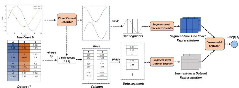
Figure 1. An overview of Fine-grained Cross-modal Relevance Learning Model (FCM).

3.1. A Proper Definition of $Rel(D,T)$

Since the underlying data $D$ and the dataset $T$ contain multiple data series, we define $Rel(D,T)$ in a bottom-up manner.

Low-level Relevance seeks to quantify the relevance $rel(d,C)$ between a column $C\in T$ and a data series $d\in D$. Each data series $d$ consists of two sequences of values, x-values and y-values, while $C$ is a single data series. When measuring the relevance between $C$ and $d$, we ignore the x-values in the data series for two reasons: (1) Users may wish to identify historical data trends similar to the current data, so the x-values might be misleading in this case; (2) As described in Sec. 2, sometimes x-values are not provided in datasets and are generated automatically by the visualization tool. Thus, measuring $rel(d,C)$ can be reduced to measuring the relevance between the column $C$ and the y-values of $d$. To achieve this, we use dynamic time warping (DTW) distance (Faloutsos et al., 1994; Ding et al., 2008; Gold and Sharir, 2018), which is widely used to deal with data sequences that have varying lengths or temporal resolutions when measuring the distance between two data series. Note that we do not use Euclidean Distance (ED) since ED cannot capture data shifts. Specifically, for a pair $(d,C)$, the relevance score is defined as $rel(d,C)=\frac{1}{1+dist(d,C)}$, where $dist$ is the DTW distance function. A larger DTW between $d$ and $C$ implies a lower relevance between the two datasets.

High-level Relevance seeks to quantify the relevance between $D$ and $T$. To achieve this, it is crucial to establish the relationship between each column in $T$ and each data series in $D$. Drawing inspiration from prior work on schema matching (Fan et al., 2023), we formulate our problem as a weighted maximum bipartite matching problem (Tanimoto et al., 1978). Here, each data series is regarded as a node in a bipartite graph $\mathcal{B}=\{\mathcal{V},\mathcal{E}\}$ and $rel(d_{i},C_{j})$ is the weight of the corresponding edge $(i,j)$ in $\mathcal{B}$. The objective is to identify a subset of edges, denoted as $\mathcal{B}^{\prime}\subseteq\mathcal{B}$, which maximizes the weighted sum, subject to the constraint that no two edges in $\mathcal{B}^{\prime}$ share a common node. Once $\mathcal{B}^{\prime}$ is determined, we can establish the mapping between the data series in $D$ and the columns in $T$. Then, the high-level relevance is computed as the sum of the weights of the selected edges, formulated as $\mathcal{B}^{\prime}$: $Rel(D,T)=\sum_{(i,j)\in\mathcal{E}}rel(d_{i},C_{j})x_{ij}$, subject to 1) $\sum_{j:(i,j)\in\mathcal{E}}x_{ij}\leq 1,\forall d_{i}\in D$, and 2) $\sum_{i:(i,j)\in\mathcal{E}}x_{ij}\leq 1,\forall C_{j}\in T$, where $x_{ij}\in\{0,1\},\forall(i,j)\in\mathcal{E}$. Note that the maximum bipartite matching problem can be solved by Hungarian algorithm (Kuhn, 1955) with a time complexity of $O(|\mathcal{V}|^{3})$.

3.2. Key Idea

We first illustrate how to match a line chart with a candidate dataset in an ideal way, using the following example.

Example 0.

As illustrated in Fig. 1, the line chart $V$ contains two lines and the dataset $T$ has three columns. To match the chart with a dataset, we may want to know whether each line in the chart can be generated from the column in the dataset. To resolve this, we first try to match each line and each column, finding that Line 1 matches column A exactly while both Column B and Column C do not match Line 2. However, when we divide Line 2, Column B, and Column C into four segments (shown in different colors and separated by dots), the initial three-quarters of Line 2 exactly align with Column B, but none of the segments in Column C correspond to any part of Line 2.

This example underscores the importance of locality matching as well as fine-grained matching when attempting to match a line chart with a dataset. Specifically, the matching is performed at two different levels: (1) At the line-to-column level, the comparison between each line and each column is performed; (2) At the segment-level, the comparison between a line segment and a data segment is carried out. This fine-grained matching process guides the design of our model when computing $Rel^{\prime}(V,T)$ – the model should have the ability to learn representations from a line chart and a dataset that can preserve locality (segment-level) information and align the segments from a line chart with a column during the matching process.

3.3. Solution Overview

Based on this idea, we propose a novel Fine-grained Cross-modal Relevance Learning Model (FCM). Fig. 1 provides an overview of our model, consisting of four components:

• Visual Element Extractor extracts informative visual elements relevant to dataset discovery via line charts task. The lines and the y-axis ticks, extracted from a line chart $V$, serve as input to subsequent components: the lines are sent to an encoder to learn the representation of the line chart $V$; the y-axis ticks are used to filter columns from a candidate dataset $T$. (Sec. 4.1)

• Segment-level Line Chart Encoder specializes in learning the representation of a line chart $V$ at the segment level. Here, a segment pertains to a line segment, containing the local context information derived from a line. (Sec. 4.2)

• Segment-level Dataset Encoder learns the representation of a candidate dataset $T$ at the segment level. Here, a segment refers to a consecutive range of data points in a column. (Sec. 4.3)

• Cross-modal Matcher learns a fine-grained alignment between a line chart and a dataset based on the learned representations at two levels, the line-to-column level and the segment level, and outputs a score to estimate the relevance. (Sec. 4.4)

Extension to Handle Aggregation-based Queries. In practice, data aggregation (DA) operations are usually used when generating a line chart. To handle aggregation-based queries, we incorporate three innovative DA-related layers into the dataset encoder to learn a comprehensive and accurate representation capable of capturing data aggregation operations, as illustrated in Fig. 3. (Sec. 5)

Hybrid Indexing Strategy. Furthermore, we also propose a hybrid indexing strategy using an interval tree (Kriegel et al., 2000) and locality-sensitive hashing (Lv et al., 2007) to improve the search efficiency at the query stage. (Sec. 6)

4. Cross-modal Relevance Modeling

4.1. Visual Element Extractor

As shown in Fig. 1, the first step of FCM is to extract informative visual elements from the line chart $V$. This serves as a pivotal step in FCM, conferring several advantages: 1) it allows the model to focus on pertinent visual elements, filtering out the influence of non-relevant ones; 2) by extracting each distinct visual element, such as individual lines from the line charts, a fine-grained matching process between the line chart and the prospective dataset becomes feasible. Specifically, for the extracted ticks, we utilize only the y-ticks as the essential visual elements, as they provide key information about the range of possible values. We do not leverage x-ticks in this task for two reasons: (1) our objective often involves the discovery of historical data analogous to the query, without necessitating specific constraints on the corresponding x-axis values within candidate datasets; (2) as previously outlined in Sec. 2, instances exist where the values on the x-axis are automatically generated and are a part of the original datasets.

To extract the two essential visual elements from $V$, we can resort to existing image segmentation methods (Minaee et al., 2021; Kirillov et al., 2023), which have been widely employed in computer vision. When applying image segmentation in our task, there are two options: 1) Direct utilization of a pre-trained large image segmentation model; 2) Training a segmentation model from scratch. However, when we tried to use SAM (Kirillov et al., 2023), one of the most powerful pre-trained image segmentation methods, to extract visual elements in a line chart, the results were not promising, achieving a mean average precision of only 0.45. One possible reason is that the training images used during the pre-training stage are much different from our case, i.e., line charts. Hence, we train our image segmentation method from scratch. However, we currently lack a dataset specifically tailored for segmenting objects within line charts. Creating such a dataset manually would be costly in terms of both labor and curation, as it would require annotating class information for every pixel in each image. To address this issue, we introduce LineChartSeg, the first dataset designed for line chart segmentation. LineChartSeg is generated by automatically labeling pixel-level information using visualization libraries, which offer insights into pixel rendering when generating a chart image. Furthermore, we propose a novel data augmentation method tailored to effectively train a line chart segmentation model (LCSeg).

LineChartSeg. We use Plotly (Hu et al., 2019), a vast real-world dataset extensively utilized in data visualization, to construct the LineChartSeg dataset. Plotly contains millions of tabular datasets, each associated with a visualization specification describing how to utilize the table columns for creating the visualization. Our approach generates a training example in LineChartSeg based on each (table, visualization specification) pair. In the image segmentation, a typical training example includes an input image requiring segmentation and a set of masks representing pixel-level class information. To create our training examples, for each table, we use the corresponding visualization specification to generate a line chart using matplotlib (Hunter, 2007), a popular visualization library. In matplotlib, each visual element is described using an artist class, such as axis, label, and line. Using the transdata method in matplotlib, we can obtain the pixel coordinate location for each artist. This allows us to generate masks for the input image by assigning distinct colors to each visual element.

Data Augmentation for Segmentation Model Training. We utilize LineChartSeg to train our line chart segmentation model (LCSeg) using a Mask RCNN (He et al., 2017), a robust image segmentation model widely applied in computer vision.

When training an image segmentation model, the incorporation of data augmentation methods is essential to achieve the full potential from each training example. However, conventional data augmentation techniques may not be suitable for our task as they can alter the semantic meaning of the chart. For instance, common methods such as flipping (He et al., 2017), which horizontally or vertically mirrors images, are not appropriate since flipping the chart image may distort key information, such as labels and ticks, diminishing informativeness.

To resolve this challenge, we propose a novel data augmentation method to train LCSeg. Our key idea is to perform data transformations on the original tabular datasets from which the line chart is originated. This new strategy not only preserves the integrity of the line chart but also enables the generation of line chart images that adhere closely to real data without modification, avoiding deviations from exemplars. Specifically, we propose the following data augmentations methods:

• Reverse. For each column $C=(a_{1},...,a_{n})$ in a dataset, we reverse all data in the column to form a new column $C^{\prime}=(a_{n},...,a_{1})$.

• Partitioning. Each column $C=(a_{1},...,a_{n})$ in a dataset is randomly partitioned at position $n^{\prime}$, to yield two columns $C_{1}^{\prime}=(a_{1},...,a_{n^{\prime}})$ and $C_{2}^{\prime}=(a_{n^{\prime}+1},...,a_{n})$.

• Down-Sampling. Each column $C=(a_{1},...,a_{n})$ in a dataset is down-sampled to contain $c$ at a ratio of $\frac{1}{\rho}$, such that in the resulting column $C^{\prime}$, only one data point is retained for every $\rho$ consecutive data points in $C$.

4.2. Segment-level Line Chart Encoder

The line chart encoder is designed to learn the representation of a line chart while preserving its segment-level information. Given a line chart $V$, we have used the visual element extractor to extract each line from the chart. Each line $l$ is then represented as a 2-D image, denoted as $I\in\mathbb{R}^{H\times W\times Q}$, where $H$ and $W$ represent the height and width of the image, and $Q$ denotes the number of color channels (e.g., red, green, and blue). While color channels are vital in traditional computer vision tasks such as image classification (He et al., 2016) and object detection (He et al., 2017), they have minimal impact in our task, which focuses primarily on the line shape. Thus, for each line $l$, we uniformly transform the chart into a greyscale image, denoted as $I_{grey}\in\mathbb{R}^{H\times W}$. This transformation reduces the input data size by a factor of $Q$, hence improving processing efficiency.

As shown in the lower left section of Fig. 2, each line is divided into a sequence of small 2-D images of line segments $I_{grey}=\{z_{1},z_{2},...,z_{N_{1}}\}$, $z_{i}\in\mathbb{R}^{H\times P_{1}}$, where $P_{1}$ denotes the width of each small image, and $N_{1}=\frac{W}{P_{1}}$ is the resulting number of small images. To learn representations for these line segment images, we apply a Vision Transformer (ViT) (Han et al., 2022; Dosovitskiy et al., 2020), which is a transformer-based architecture that encodes the image features. Each line segment image $z_{i}$ is flattened into a 1-D vector of length $WP_{1}$, which is then transformed into a vector of length $K$ using a trainable linear projection layer. Here, $K$ denotes the embedding size.

Using the above procedure, a line image $I$ is transformed into a sequence of embedding vectors. Then, the encoder applies a standard transformer to further encode the sequence, enabling an encoder to learn correlations between the line segments. The transformer encoder consists of $J$ multi-head self-attention (MSA) and multi-layer perceptron (MLP) blocks, and processes a line $l$ as follows:

(2) $$u_{0}= [z_{1};z_{2};...;z_{N_{1}}]+E_{pos}, E_{pos}\in\mathbb{R}^{N_{1}\times K},$$

$$u^{\prime}_{i}= MSA(LN(u_{i-1}))+u_{i-1}, i=1,...,J,$$

$$u_{i}= MLP(LN(u^{\prime}_{i}))+u^{\prime}_{i}, i=1,...,J$$

Here, $LN$ denotes the layernorm, a technique employed to normalize the input and expedite model convergence; $E_{pos}$ are positional embeddings that are trainable parameters and encode positional information for the line segments in line $l$.

As a result, $u_{J}\in\mathbb{R}^{N_{1}\times K}$ is the representation for a line, where each row in $u_{J}$ corresponds to the representation of a line segment. Note that there are $M$ lines in a line chart. Therefore, for the entire line chart $V$, we combine all of the representations of the lines contained in $V$, leading to a final representation $E_{V}\in\mathbb{R}^{M\times N_{1}\times D}$ for the line chart $V$. For simplicity, we use $E_{V}[i]$ to denote the representation of the $i$-th line in $V$, and $E_{V}[i,j]$ to denote the representation of the $j$-th segment of the $i$-th line in $V$.

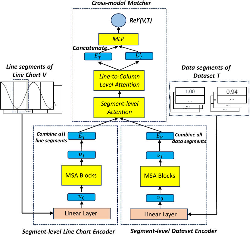
Figure 2. The architecture of the segment-level encoders and the cross-modal matcher.

4.3. Segment-level Dataset Encoder

For each dataset $T$, we first leverage information from the y-axis ticks in an image to determine the range of values of the data and filter columns in $T$. Subsequently, the dataset encoder focuses on learning a segment-level representation for each remaining column $C$. Specifically, each column $C$ can be represented by a data series $C=(a_{1},a_{2},...,a_{N_{R}})$ where $a_{i}$ denotes the content of $i$-th cell in $C$. We partition $C$ into $N_{2}$ segments, $C=(w_{1},w_{2},...,w_{N_{2}})$, where each $w_{i}$ contains $P_{2}=\frac{N_{R}}{N_{2}}$ data points (cell values). Then, a transformer-based architecture can be applied to learn a representation for each data segment. In addition to preserving local semantics and facilitating fine-grained matching, this process also improves efficiency. Specifically, partitioning a column (of length $N_{R}$) into $N_{2}$ segments results in measurable memory and time savings – approximately a factor of $(P_{2})^{2}$ – when computing self-attention, which is a crucial component in the transformer-based encoder since the time and space complexity of self-attention are quadratic w.r.t. the length of the input sequence.

The lower right of Fig. 2 shows the architecture of the segment-level dataset encoder. First, each data segment $w_{i}$ is mapped to a vector $v_{0}$ of length $K$ using a trainable linear projection layer. The output is then fed into a standard transformer to derive the final representation for each data segment of column $C$. This process is similar to the line chart encoding, and for brevity, we do not repeat those details here. Ultimately, the representation for each data segment across every column in $T$ is combined into a final representation, denoted as $E_{T}\in\mathbb{R}^{N_{C}\times N_{2}\times D}$, where $N_{C}$ denotes the number of columns in $T$. Similarly, $E_{T}[m]$ denotes the representation of the $m$-th column in $T$, and $E_{T}[m,n]$ denotes the representation of the $n$-th segment of the $m$-th column of $T$.

4.4. Cross-modal Matcher

Given representations $E_{T}$ and $E_{V}$, the cross-modal matcher estimates the relevance score $Rel^{\prime}(V,T)$ at two levels: the line-to-column level and the segment level, as outlined in Sec. 3.2. To achieve this, we propose a hierachical cross-modal attention network (HCMAN) to implement the matcher. As shown at the top of Fig. 2, HCMAN has two levels of self-attention networks, each designed to capture the relevance between elements at their respective level.

Specifically, given two representations for a line chart and the target dataset, $E_{V}$ and $E_{T}$, HCMAN matches each line segment representation $E_{V}[i,j]$ and each data segment representation $E_{T}[m,n]$ with a segment-level self-attention network (SL-SAN). SL-SAN first transforms each column segment representation or line segment representation into three distinct vectors: a query vector $p_{q}$, a key vector $p_{k}$, and a value vector $p_{v}$. Then, the relevance score between $E_{V}[i,j]$ and $E_{T}[m,n]$ is computed using $sim(p_{q}(E_{V}[i,j])$, $p_{k}(E_{T}[m,n]))$, where $sim$ is a scaled dot-product similarity function (Vaswani et al., 2017). Depending on the relevance score returned, the line (column) representation $E_{V}^{\prime}[i]$ ($E_{T}^{\prime}[m]$) is reconstructed using the relevance-weighted sum of all the corresponding line (data) segments.

Following segment-level matching, HCMAN matches each line representation $E_{V}[i]$ with each column representation $E_{T}[m]$ using line-to-column level self-attention (LL-SAN). Similar to the segment-level process descibed above, LL-SAN uses self-attention to compute the relevance between each line and each column, and reconstructs the line chart representation $E_{V}^{\prime}$ and the dataset representation $E_{T}^{\prime}$ using the relevance-weighted sum of all the lines and columns, respectively.

In the final step, the reconstructed representation of the line chart and the dataset, $E^{\prime}_{V}$ and $E^{\prime}_{T}$, are concatenated and then passed through an MLP to learn a relevance score $Rel^{\prime}(V,T)$.

5. Handling Data Aggregation-based Queries

In practical scenarios, users often generate line charts using aggregated data from datasets. For instance, daily sales figures may be aggregated to calculate total monthly sales revenue. Thus, our objective is to enhance FCM to support data aggregation (DA)-based line chart queries. Handling DA-based queries poses a greater challenge since the aggregated data used to construct the line chart can vary significantly from the original datasets. Therefore, directly applying FCM descibed above to match candidate datasets with DA-based line charts would result in poor performance due to the substantial differences between the aggregated data and the original dataset.

Moreover, the potential valid data aggregation operations for a given dataset can be extensive due to arbitrary aggregation window sizes and numerous aggregation operators. To tackle this issue, we propose an enhancement of FCM by introducing three additional layers in the dataset encoder:

• Hierarchical Multi-scale Representation Layer (HMRL) is proposed to capture localized characteristics associated with aggregating over a particular window size.

• Transformation Layer is designed to address distribution shift between the raw candidate dataset and any aggregated data.

• Mixture-of-Experts Layer (Yuksel et al., 2012) is employed to automatically infer the most probable data aggregation operator.

5.1. Hierarchical Multi-scale Representation Layer

As introduced in Sec. 4.3, the segment-level dataset encoder learns the dataset representation in a segment-level, which is achieved by partitioning each column into several data segments. Ideally, matching the data segment length with the aggregation window size would be optimal, but this is nearly infeasible given the arbitrary nature of aggregation window sizes. To overcome this challenge, we propose the integration of segment-level representations with multi-scale information present in the columns, through the introduction of the novel hierarchical multi-scale representation layers (HMRLs). This involves further subdividing a segment $w$ with a length of $N_{1}$ (as described in Section 4.3) into smaller segments. A tree structure is then employed to facilitate the learning of multi-scale segment representations in a bottom-up fashion. This hierarchical approach ensures that higher-level representations of segments incorporate information from their corresponding lower-level segments.

Specifically, as illustrated in Fig. 3, in HMRLs, each segment in the original dataset encoder is first divided into $2^{\beta}$ smaller segments, and then the smallest segments are organized in the leaf nodes of a binary tree. Nodes at higher levels correspond to larger segments. The $j$-th node in the $i$-th layer of the binary tree is denoted as $e_{i,j}$. For any non-leaf node $e_{i,j}$ in the binary tree, its representation can be obtained as a function of the representations of its two children, i.e., $e_{i,j}=f(left(e_{i,j}),right(e_{i,j}))$, where $right(\cdot)$ and $left(\cdot)$ denote the right child and left child of a node in the binary tree, respectively. Here, an MLP is chosen as the function $f$. Consequently, information at different scales is incorporated by the top node $e_{\beta,0}$. Next, we will introduce the process of obtaining the inital representation of the smallest data segment in the leaf node.

5.2. Transformation Layers

A data aggregation operator involved in a line chart can alter the distribution of the original dataset $T$, potentially causing a mismatch between $D$ and $T$. Considering each data aggregation operator as a transformation from $T$ to $D$, we propose transformation layers to capture such changes. These transformation layers model the transformation based on the representations of segments in the leaf node, facilitating the propagation of the transformation in a bottom-up manner. To achieve this, we employ a two-layers MLP to transform $c$ into the representation of the smallest segment at the leaf node, denoted as $e_{0}$.

For each data aggregation operator, an independent transformation layer is applied to model the transformation, as different aggregation operators alter the original dataset in distinct ways. Additionally, an extra transformation layer is designed to model the identity transformation for Non-DA-based line charts. Consequently, there are five different transformation layers in total.

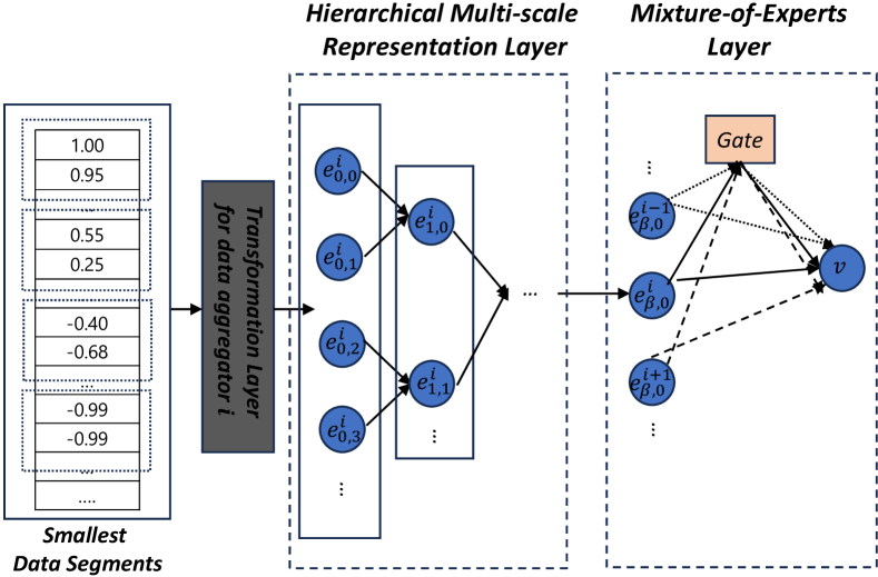
Figure 3. The architecture of the three layers for supporting aggregation-based queries.

5.3. Mixture-of-Experts Layer

We now introduce how a Mixture-of-Experts (MoE) layer (Yuksel et al., 2012; Shazeer et al., 2016) is utilized to automatically select the appropriate data aggregation operator. When dealing with a line chart $V$, no prior knowledge is available about whether it was generated using aggregation operators or which specific aggregation operator was applied. Despite introducing the transformation layer to bridge the data shift from the original data $D$ to the underlying data $T$, the model lacks information on which transformation layer to employ. To address this issue, we introduce an MoE layer into FCM. The MoE layer is widely used to combine predictions or outputs from multiple “expert” models in a weighted manner to derive a final prediction. In our context, each transformation layer is considered an expert.

For each expert model, given the five transformation layers, we obtain five different representations, denoted as $e^{0}_{\beta 0},e^{1}_{\beta 0},...e^{4}_{\beta 0}$. Then, the MoE layer obtains the representation $v$ according to $v=\sum_{i=0}^{4}g_{i}(e^{i}_{\beta,0})\cdot e^{i}_{\beta,0}.$ Here, $v$ is the final representation for the largest segment, which is then fed into the transformer architecture within the segment-level dataset encoder, as described in Sec. 4.3. $g_{i}$ denotes the gating mechanism’s output for the $i$-th expert. This output acts as a probability distribution over the experts, determining the weight of each expert’s output. Specifically, $g_{i}$ signifies the probability associated with different aggregation operators. To accomplish this, we design two fully-connected layers for each gating function $g_{i}$, using LeakyReLU and Softmax as activation functions: $g_{i}=\text{Softmax}(\text{LeakyReLU}(e^{i}_{\beta,0}W_{1}^{G})W_{2}^{G})$.

5.4. Model Training

To train the encoders and matcher in FCM, we use the negative loss as the objective function:

(3) $$\mathcal{L}=-[\frac{1}{N_{pos}}\sum_{i=1}^{K_{1}}r_{i}\cdot\log(\hat{r}_{i})+\frac{1}{N_{neg}}\sum_{i=1}^{K_{0}}(1-r_{i})\cdot\log(1-\hat{r}_{i})]$$

where $r_{i}$ denotes a ground truth label $Rel(D_{i},T_{i})$, $\hat{r}_{i}$ denotes the model output $Rel^{\prime}(V_{i},T_{i})$, $N_{pos}$ and $N_{neg}$ denote the number of positive and negative training examples in the training dataset, respectively. Given that the original training dataset only contains positive training examples, negative training examples are created using a negative sampling strategy – for each positive training pair $(V_{i},T_{i})$, we select $N^{-}$ candidate datasets from the datasets to form the negative training set for $V_{i}$.

The selection of negative training examples is crucial for FCM to learn robust and discriminative representations for the dataset and line chart. Appropriate negative examples not only expedite the convergence of training processes, but also enable the model to achieve higher effectiveness. If the negative examples are too easy – markedly different from the positive examples – FCM may not effectively learn how to discriminate significant differences in the input. This can lead to under-tuned decision boundaries which fail to capture subtle nuances in the dataset. On the other hand, excessively difficult negative samples may be so close to the positive examples in the embedding space that the model fails to distinguish between them.

To ensure effective and efficient model training, we use a “semi-hard” negative example selection criteria (Schroff et al., 2015; Luo et al., 2018). Without loss of generality, considering the use of an SGD-based optimization method to optimize our model in the training stage, a mini-batch $B$ is randomly selected from the training data in each training epoch. For each line chart in $B$, we select semi-hard negative examples. Notably, in the training stage, access to the underlying data for all line chart queries is available. Therefore, for each line chart $V$, a relevance score $Rel(D,T)$ between the underlying data and all datasets in the mini-batch $B$ is computed. Then, the datasets are ranked by the relevance score, and those with relevance scores positioned in the middle of the $N^{-}$ values are included as negative examples.

6. Query Processing and Generalization

6.1. Efficient Processing of a Line Chart Query

Once FCM has been trained, we proceed to find the top-$k$ relevant datasets to a line chart query. To achieve an efficient query processing, we employ a hybrid indexing strategy that melds interval trees with locality sensitive hashing (LSH), by identifying a compact set of promising candidate datasets.

Interval Tree. Recall Sec. 4.1, we can obtain the range of y-values from the line chart by the visual element extractor, which provides insights into the column range a candidate dataset should encompass. Hence, we first construct an interval tree to quickly find candidate datasets whose columns overlap with the given range–for each candidate dataset, We define the possible range for each column $C$ as the interval $[min(C),sum(C)]$, where the minimum and maximum values are achieved by applying the $min$ and $sum$ aggregation operators to the entire column, respectively. Then, we insert all the intervals into an interval tree and employ all the intervals of a dataset to index it.

LSH. We also leverage an LSH index to expedite the query processing, built upon the learned representations from FCM. First, we employ the dataset encoder introduced in Sec. 4.3 to obtain segment-level representations for each dataset. Then, for each column $C$ of the dataset, we derive its representation $E_{C}$ by averaging all representations of segments belonging to that column. Next, a hash function $f$ is applied to map $E_{C}$ to a binary code $B_{C}$. To obtain such a binary function $f$, we randomly generate $K$ vectors of the same length as $E_{C}$. For each generated vector, we obtain the cosine similarity between $E_{C}$ and the vector, rounding the similarity score into 0 or 1. Consequently, the binary code $B_{C}$ is obtained by combining $K$ bits of similarity scores. Note that for each dataset, it will be indexed by all binary codes of its columns.

In query processing stage, given a line chart $V$, we first employ the visual element extractor to obtain all lines and the range of y-tick values. Treating this range as an interval, we employ it as a query on the interval tree to identify the set of datasets $\mathcal{S}_{1}$ that have at least one column overlapping with the query interval. Then, for the extracted lines, we employ the line chart encoder to obtain the segment-level representations of $V$. Then for each line $l\in V$, we derive its representation $E_{l}$ by averaging representations of segments belonging to the line. Next, the hash function $f$ is applied to $E_{l}$ to transform it into the binary code $B_{l}$. Any dataset colliding with $B_{l}$ based on the binary code is added to another set $\mathcal{S}_{2}$. As a result, $\mathcal{S}_{1}\cap\mathcal{S}_{2}$ contains datasets requiring further verification. For each dataset $T\in\mathcal{S}_{1}\cap\mathcal{S}_{2}$, FCM is employed to calculate the relevance score $Rel^{\prime}(V,T)$, which serves as the reference to find the top-$k$ datasets.

6.2. Generalization of FCM

Generalization to Line Charts with Numerical X-axis. In the early part of this work, we assume that the underlying data along the x-axis are evenly distributed, which is often the case when the x-axis represents time stamps or disrecte steps. However, there exist rare cases when the x-axis values are numerical and not evenly distributed. To address this, FCM can be adapted with two modifications: (1) For each column $C$ in a candidate dataset $T$, we treat it as a potential x-axis value. Then we sort all rows using $C$ as a reference and apply interpolation to make $C$ evenly distributed. This allows FCM  to estimate the relevance between the derived dataset and the line chart. We denote the derived table as $T^{\prime}$. Since there are $N_{C}$ possible $T^{\prime}$ datasets for each $T$, we select the one with the highest relevance score as the final score $Rel^{\prime}(V,T)$. (2) Similarly, for the indexing strategy, for each $T^{\prime}$ derived from $T$, we need to add all the intervals into the interval tree to index the candidate dataset $T$, and add each corresponding hash code of $T^{\prime}$ to index $T$.

Generalization to Other Types of Charts. While our primary focus is on learning a relevance score $Rel^{\prime}(V,T)$ between a line chart and a dataset, our solution can be extended to support a variety of other chart types, such as bar charts, pie charts or scatter charts, with only small adjustments: (1) Employ the visual element extractor to extract the essential visual elements from other chart types, such as sectors in a pie chart, bars in a bar chart, colored data point series in a scatter chart. Note that the visual element extractor should be retrained on relevant datasets. (2) Adjust or remove the way of segmenting the visual elements, i.e., sectors, bars, and data point series. For instance, it is meaningless to further segment a bar and a sector while we can follow the same method in this paper to segment a data point series. (3) Determine an appropriate relevance metric to estimate the relevance between the underlying data and dataset, which is important to create the training dataset and identify the training examples. For instance, since a pie chart commonly depicts a data distribution, metrics such as KL-Distance may be more appropriate to compute $Rel(D,T)$. Notably, handling certain types of charts is less challenging than line charts for two reasons: 1) The patterns in the charts may exhibit more regularity, facilitating easier representation learning by the model. 2) These charts either do not involve data aggregation (e.g., scatter charts) or have a small number of possible aggregation operations (e.g., pie charts), while line charts can use a large number of aggregation operations due to number of possible window sizes.

Table 1. Statistical properties of our benchmark.

	Overall	Number of Lines $M$
		$1$	$2-4$	$5-7$	$>7$
Query	200	74	48	44	34
Repository	10,161	3,658	2,540	2,134	1,829

7. Experiments

7.1. The Benchmark

As this work is the first to explore the dataset discovery via line charts problem, we create a benchmark using data sourced from Plotly (Hu et al., 2019), a widely used dataset in data visualization (Zhou et al., 2021). Plotly contains 2.3 million records, each represented as a (table, visualization configuration) pair. The visualization configuration specifies which columns from a table and which chart type are used for the visualization. Specifically, we process the Plotly data as follows, and Table 1 shows essential statistical propoerties:

• Data Filtering and Deduplication. Records whose datasets are not visualized using line charts are excluded, and only one record is kept if multiple near-duplicate tables exist in the records.

• Table Extraction. For each record, the table is extracted and a collection of related tables $\mathcal{D}$ is created.

• Data Split. The remaining tables are divided into a training set $T_{train}$, a validation set $T_{val}$, and a test set $T_{test}$. Specifically, $3{,}000$ and $1{,}000$ tables are randomly selected from $\mathcal{D}$ to form $T_{train}$ and $T_{val}$, respectively. $T_{train}$ is also used to create the dataset LineChartSeg, as described in Sec. 4.1. Furthermore, for each table in $T_{train}$ and $T_{val}$, the associated visualization specification is used to create a triplet $(V,D,T)$, as discussed in Def. 2.2.

• Query Selection. A total of $100$ tables are randomly selected as $T_{test}$ to construct the line chart queries. For each table, two types of line charts are generated: one based on the corresponding visualization configuration; another using data aggregation. The data aggregation is applied by randomly selecting one of the four aggregation operators described in Sec. 2. Additionally, the aggregation window size is chosen uniformly at random from the range $min(100,N_{R}/10)$, where $N_{R}$ is the number of rows in the table.

• Ground-truth Generation. First, for each line chart query, we inject small noises into the data for each corresponding table $T$ of $V$ to create 50 new tables $T^{\prime}$. For each column $C\in T$ (excluding the column matching the x-axis), noise is added using $C_{new}=C\times\sigma$, where $\sigma$ is a vector of the same length as $C$, and each element in $\sigma$ follows a uniform distribution $U\sim(0.9,1.1)$. These new tables $T^{\prime}$ are then added into the repository $\mathcal{T}$. In this way, we can ensure that the repository contains enough datasets that are similar to each line chart query. Then, for each $V$, the relevance score $Rel(D,T)$ (introduced in Sec. 3.1) is computed to find the top-50 tables, forming the relevant datasets.

7.2. Experimental Settings

Baselines. As this is the first study on dataset discovery via line charts, no known methods can directly solve it. Hence, we establish the following baselines to compare with our FCM:
(1) CML. This is a simple but effective baseline, which adopts the state-of-the-art image and table encoders, a Vision Transformer (Han et al., 2022) and TURL (Deng et al., 2020), to learn representations for line charts and datasets, respectively. Then, the cosine similarity is used to compute $Rel^{\prime}(V,T)$ based on the learned representations.
(2) Qetch*. Qetch (Mannino and Abouzied, 2018a) is a sketch-based time series search method, which finds time series segments similar to a single sketched line. To extend this approach to handle queries containing multiple lines, we apply a visual element extractor to extract all of the lines from the line chart, and compute the relevance between each extracted line and each column from the candidate dataset using the matching algorithm proposed for Qetch in the original paper. Then the relevance between a dataset and a line chart is obtained by aggregating all of the relevance scores between each line and each column using maximum bipartite matching, as outlined in Sec. 3.1. We denote this version of Qetch as Qetch*.
(3) DE-LN. We combine state-of-the-art visualization recommendation (VisRec) and visualization retrieval methods, DeepEye (Luo et al., 2018) and LineNet (Luo et al., 2023), as another baseline to solve our problem. For each candidate dataset in the repository, we apply DeepEye to generate a list of 5 line chart candidates. Then, we apply LineNet to compute the similarity between the recommended line charts and the line chart query. Then the highest similarity score serves as the relevance score $Rel^{\prime}(V,T)$.
(4) Opt-LN. To minimize the impact of the VisRec method on the model effectiveness, we adopt Opt-LN as a method to represent the upper bound performance of the method which combines visualization recommendation and LineNet. Opt-LN applies LineNet to directly compute the relevance score $Rel^{\prime}(V,T)$ between a line chart query and the candidate dataset from Plotly associated with the line chart query. Note that this method is not possible in practice but serves solely as an upper performance bound for DE-LN.

Evaluation Metrics. Since this is inherently a search problem, we use prec@k and ndcg@k to measure effectiveness. prec@k measures the accuracy of the top-$k$ list by counting the number of correctly predicted relevant datasets in the top-$k$ datasets returned, and ndcg@k measures how well a ranked list performs by the positional relevance. In this work, since the number of relevant datasets available for each line chart query is 50 (see Sec. 7.2), we set $k$=50.

Model Configuration. For the transformers used in FCM, the number of transformer encoder layers and multiple attention heads are set to $12$ and $8$, respectively. The dimensionality of the transformer is set to $768$ by default. The line segment and column segment sizes are set to 60 and 64, respectively. The number of negative samples $N^{-}$ is set to $3$ by default. We use the Adam optimizer with a learning rate of $10^{-6}$ and train FCM for $60$ epochs.

Environment. We conducted all experiments on an Ubuntu server with an Intel Core i7-13700K CPU and an RTX 4090 GPU with 24 GB of memory. The code will be publicly released after the paper is accepted. We have also implemented a system prototype (Ji et al., 2024).

7.3. Top-k Effectiveness

Effectiveness using All Queries. Table 2 reports the average prec@50 and ndcg@50 of all methods using all of the queries, with a per query breakdown with and without data aggregation. Our FCM achieves the best overall performance across all queries and metrics. When compared against the best baseline CML, the relative improvement is $30.1\%$ and $41.0\%$ in terms of prec@50 and ndcg@50, respectively. CML also demonstrates the ability to locate relevant datasets, marginally outperforming Opt-LN. Note that both CML and our FCM are using a transformer-based architecture for the encoders for both line charts and datasets. This reinforces a commonly held belief in the ML community that transformers are effective on learning accurate and comprehensive representations for different data modalities. Moreover, FCM outperforms Qetch* significantly. One possible reason is that Qetch is mainly designed to match local patterns and is not suitable when matching global patterns, and the heuristic matching algorithm is not as effective as deep learning-based methods on aligning the features of line charts and datasets. Finally, Opt-LN outperforms DE-LN significantly, since the performance of DE-LN is bounded by the recommendation accuracy.

Table 2. Effectiveness for all queries and queries with/without data aggregation (DA)

	Metrics	CML	DE-LN	Opt-LN	Qetch*	FCM
Overall	prec@50	0.349	0.224	0.287	0.256	0.454
	ndcg@50	0.246	0.162	0.211	0.179	0.347
With DA	prec@50	0.180	0.134	0.160	0.123	0.398
	ndcg@50	0.119	0.098	0.118	0.105	0.302
Without DA	prec@50	0.538	0.318	0.417	0.390	0.589
	ndcg@50	0.372	0.226	0.303	0.246	0.456

Effectiveness of Multi-line Queries. Table 3 reports the results on queries with a varying number of lines. Our FCM consistently achieves the best performance. As the number of lines $M$ increases, the relative improvement percentage of FCM over the best baseline CML also increases. Concretely, when $M$ falls into different ranges: 1, 2-4, 5, 6, $\textgreater$7, FCM surpasses CML by 25.7%, 29.1%, 33.4%, and 36.6% in terms of prec@50, respectively, while the ndcg@50 of FCM surpasses CML by 34.8%, 38.6%, 45.8%, and 51.3%, respectively. The key reason is that FCM includes an effective line chart segmentation method (introduced in Sec. 4.1), which can extract the shape of the lines from the line chart query, and applies a finer-grained matching in the search process. This leads to superior performance for line charts containing multiple lines.

Table 3. Overall effectiveness w.r.t. varying $M$.

$M$	Metrics	CML	DE-LN	Opt-LN	Qetch*	FCM
$1$	prec@50	0.453	0.328	0.431	0.344	0.569
	ndcg@50	0.327	0.240	0.316	0.239	0.441
$2-4$	prec@50	0.384	0.192	0.262	0.276	0.496
	ndcg@50	0.297	0.136	0.188	0.187	0.413
$5-7$	prec@50	0.283	0.174	0.194	0.141	0.378
	ndcg@50	0.187	0.125	0.147	0.125	0.275
$>7$	prec@50	0.175	0.104	0.127	0.121	0.240
	ndcg@50	0.092	0.073	0.096	0.082	0.140

Effectiveness of DA-based Queries. FCM also demonstrates excellent performance on DA-based queries, achieving a prec@50 of $0.398$ and an ndcg@50 of $0.302$, outperforming the best baseline, CML, by $121.1\%$ and $153.7\%$, respectively. Furthermore, DA-based queries appear to be much more challenging than non-DA-based queries, as evidenced by the performance drop in all the methods (see Table 2). Nevertheless, FCM is affected the least. In a further breakdown of 100 aggregation-based queries, categorized by the aggregation type: $min$, $max$, $sum$, and $mean$, along with the aggregation window size, using prec@50 is shown in Table  4. Observe that: (1) FCM excels in handling $sum$ and $mean$ aggregated queries, as compared to $min$ and $max$ aggregation queries. This could be attributed to the transformation layer’s ability to learn behaviors associated with $sum$ and $mean$ operations more effectively. (2) When using small aggregation window sizes (i.e., $0-60$), FCM exhibits stable performance. However, when the window size exceeds $60$, the performance of FCM begins to degrade sharply. This is because the aggregation window size exceeds the dataset segment size $P_{2}$ (e.g., 64), preventing FCM from capturing the localized characteristics based on the window size. Increasing $P_{2}$ is a straightforward solution, but as discussed in Sec. 9, this leads to an overall decrease in model performance.

Table 4. Breakdown of DA-based Queries using prec@50

	Aggregation Window Size
	$0-10$	$20-40$	$40-60$	$60-80$	$80-100$
$min$	0.351	0.336	0.360	0.282	0.272
$max$	0.368	0.345	0.372	0.265	0.270
$sum$	0.418	0.446	0.450	0.313	0.275
$mean$	0.454	0.416	0.439	0.337	0.317

7.4. Effectiveness of Visual Element Extraction

We further verify: 1) how the proposed LineChartSeg (in Sec. 4.1) improves the performance for the line chart segmentation task; 2) how the proposed data augmentation methods (Sec. 4.1) improve the performance of LCSeg.

To accomplish these goals, LCSeg is compared against two alternatives: (1) SAM (Kirillov et al., 2023) – a state-of-the-art pre-trained image segmentation algorithm; (2) LCSeg* – an alternative version of LCSeg which uses common data augmentation methods, such as flipping and cropping (He et al., 2017) when training the model. Two additional evaluation metrics are included in this study – Mean Average precision (MAP) and Accuracy. MAP is widely used to evaluate the image segmentation, and Accuracy measures the percentage of lines that are accurately extracted from the line charts.

Table 5 shows the results of line chart segmentation. LCSeg achieves the highest scores for both MAP and Accuracy. When compared against SAM, the relative improvement is 64.1% and 120.4% on MAP and Accuracy, respectively. This highlights a significant difference between the images in the pre-training of SAM and the line charts, underscorimg the necessity of a new dataset, such as LineChartSeg, to train more effective models for visual element extraction. Moreover, when compared against LCSeg*, LCSeg has relative improvements of 15.7% and 22.5% on MAP and Accuracy, respectively. This provides additional evidence that the effectiveness of our data augmentation algorithm for visual element extraction tasks outperforms conventional image segmentation algorithms.

Table 5. Effectiveness on visual element extraction

	SAM	LCSeg*	LCSeg
MAP	0.45	0.63	0.74
Accuracy	0.29	0.52	0.64

7.5. Ablation Study

7.5.1. Impact of Hierachical Cross-modal Attention Network

To verify the effectiveness of using a hierarchical cross-modal attention network (HCMAN), an alternative version of FCM is included, called FCM-HCMAN, containing the following changes: (1) For the line chart encoder, embeddings for line segments are averaged to derive a new representation for each line. Then, the representations for all the lines are averaged to generate a final representation for each line chart. (2) For the dataset encoder, embeddings for all data segments of a column are averaged to obtain a representation for each column. These column representations are then averaged to yield the final representation for a dataset. Then, the representations from all of the columns are averaged to obtain the final representation for each dataset. (3) For the matching, instead of using HCMAN, the representations from the line chart and dataset are concatenated into one representation, which are fed into a Multilayer Perceptron (MLP) to learn a relevance score.

Table 6. Effectiveness of FCM vs FCM-HCMAN

$M$	FCM		FCM-HCMAN
	prec@50	ndcg@50	prec@50	ndcg@50
Overall	0.454	0.347	0.368	0.267
$1$	0.569	0.441	0.480	0.353
$2-4$	0.496	0.275	0.404	0.322
$5-7$	0.378	0.235	0.298	0.206
$>7$	0.240	0.140	0.182	0.101

Table 6 compares the results for FCM and FCM-HCMAN using prec@50 and ndcg@50. FCM consistently outperforms FCM-HCMAN, with an improvement of 23.3% and 29.5% on prec@50 and ndcg@50, respectively. Furthermore, as $M$ increases, the relative improvement also increases. This provides further evidence of the effectiveness of the hierarchical cross-modal attention network provides finer-grained matching between a line chart and a dataset.

Table 7. Impact of data aggregation (DA) related Layers

	Metrics	Overall	With DA	Without DA
FCM	prec@50	0.454	0.398	0.589
	ndcg@50	0.347	0.302	0.456
FCM-DA	prec@50	0.385	0.175	0.595
	ndcg@50	0.287	0.116	0.458

7.5.2. The Impact of Data Aggregation (DA) Layers

To validate the value of including the three DA layers, another variant of FCM, called FCM-DA, is created by removing these layers from the model.

Table 7 presents prec@50 and ndcg@50 for FCM and FCM-DA. Observe that FCM outperforms FCM-DA with a relative improvement of 18.5% when using all of the queries. For DA-based queries, FCM achieves a prec@50 score of 0.454 and an ndcg@50 of 0.347, outperforming FCM-DA substantially, with improvements of 120.8% and 159.2%, respectively. For non-DA-based queries, the performance of FCM is very similar to FCM-DA. This experiment demonstrates that involving the three DA layers greatly enhances the model ability to support DA-based queries, while retaining the effectiveness on non-DA-based queries.

7.6. Hyper-parameter Study

7.6.1. Impact of the Number of Negative Instances $N^{-}$

Table. 8 shows the model performance as $N^{-}$ varies, using prec@50 and ndcg@50. When $N^{-}$ increases from 1 to 3, both prec@50 and ndcg@50 exhibit a steady increase, demonstrating that we need a sufficient number of negative training examples for maximum model performance. When $N^{-}$ increases from 3 to 6, prec@50 and ndcg@50 begin to stabilize. However, as we continue to increase $N^{-}$, the model performance will eventually begin to degrade, since too many negative samples may increase the number of false negatives. Considering that more negative samples will increase training time, $N^{-}$=3 appears to achieve the best balance.

Table 8. The impact of the number of negative samples

	1	2	3	4	5	7	8	9	10
prec@50	0.417	0.434	0.454	0.457	0.455	0.449	0.443	0.444	0.437
ndcg@50	0.323	0.339	0.347	0.345	0.346	0.341	0.339	0.334	0.329

7.6.2. Impact of the segment sizes $P_{1}$ and $P_{2}$

To study their impact, various combinations of settings for $P_{1}$ and $P_{2}$ are tested and shown in Table 9. We find: (1) The model performance is worse when $P_{1}$ or $P_{2}$ is very large, possibly because FCM no longer captures fine-grained characteristics of the lines or columns. (2) When both $P_{1}$ and $P_{2}$ are very small, the model performance is even worse. One possible reason is when $P_{1}$ and $P_{2}$ are too small, any local characteristics of the line or column no longer exist. For example, assume that in the extreme case, when both $P_{1}$ and $P_{2}$ are 1, a line segment degenerates to a pixel and a column segment degenerates into a single data point, and no data trend is discernible at this segment size. Thus, the model only begins to achieve the best performance when both values are moderate.

Table 9. The impact of Different $P_{1}$ and $P_{2}$

		$P_{2}$
		16	32	64	128	256
$P_{1}$	15	0.384	0.392	0.414	0.407	0.405
	30	0.401	0.424	0.437	0.435	0.433
	60	0.413	0.446	0.454	0.432	0.427
	120	0.354	0.375	0.396	0.376	0.377
	240	0.334	0.348	0.357	0.343	0.312

7.7. Efficiency Study

We first run all the methods to identify relevant datasets using a simple linear scan algorithm. On average, CML, LN-DE, Qetch*, and FCM require 402s, 1034s, 119s, and 374s to identify relevant datasets for a given line chart query. Qetch* is faster than CML and FCM since both CML and FCM are deep learning-based algorithms that require substantial computational resources, while Qetch* relies only on a simple heuristic matching algorithm. LN-DE is the least effective since it requires two stages to compute the relevance score – visualization recommendation and relevance score estimation. However, none of the methods are real-time as the linear scan is computationally expensive, which necessitates the indexing methods to achieve a sub-linear time cost.

Table 10 demonstrates the impact of various indexing strategies on the model performance in terms of efficiency and effectiveness. As we can see, the interval tree helps to filter out most candidates where the columns are outside of the expected range, reducing the search time to 187s. Another advantage of the interval tree is that it will not eliminate false negatives, so it can achieve the same performance as a linear scan can. In contrast, an LSH index is able to filter even more non-relevant candidates, so the query time drops to 28s. However, LSH may be overly aggressive and can exclude relevant results, and exhibits a marginal reduction in overall effectiveness. By combining both indexing strategies, the query time can be further reduced to 12s. It requires 82 min and 135 min to build the interval tree and the LSH index, respectively, and the memory footprint for these two methods are 2.1GB and 3.8 GB, respectively. In summary, our proposed hybrid indexing method achieves a 41x efficiency gain over a linear scan, and maintains similar performance for the task of dataset discovery using line charts.

Table 10. Comparison of different indexing strategies.

	prec@50	ndcg@50	Query time (s)
No Index	0.494	0.377	374
Interval Tree	0.494	0.377	187
LSH	0.454	0.347	28
Hybrid	0.454	0.347	12

8. Related Work

Dataset Discovery aims to identify relevant datasets in a large dataset repository (e.g., data lake) to meet the user need. Depending on the type of user queries, existing approaches can be broadly divided into two categories: (1) Keywords-based dataset discovery identify a set of datasets that are relevant to a given set of keywords; (2) Joinable (Fernandez et al., 2018; Zhu et al., 2019; Santos et al., 2021) or Unionable (Nargesian et al., 2018; Santos et al., 2021; Fan et al., 2023; Bogatu et al., 2020) dataset discovery methods find datasets that can be joined or merged with a user-provided dataset. Our work studies a novel dataset discovery problem, dataset discovery via line charts, where the input is a line chart (the query) and identifies relevant datasets which could be used to generate a line chart similar to the input.

Chart Search identifies similar charts from a repository using a chart as a query. Depending the accessibility of the underlying data, existing approaches can be divided into two categories: (1) Data-based chart search  (Wang and Palpanas, 2021; Lekschas et al., 2020; Siddiqui et al., 2016) assumes that the underlying data for the chart is available as input, and used to help guide the search process; (2) Perception-based chart search  (Luo et al., 2023; Li et al., 2022a; Saleh et al., 2015; Hoque and Agrawala, 2019) primarily study how to extract informative visual features from the charts and use similarity between features to identify similar charts. Both chart search and our work use a visual chart as the primary input. However, while chart search seeks to identify similar visualizations, our problems aims to provide a collection of relevant datasets, and is considerably more complex as it requires two different data modalities to be considered.

Time Series Search. Time series uses a sequence of data points collected or recorded at regular time intervals, and is usually visualized as a line chart. A lot of work has been devoted to finding relevant time series data using different forms of user input, such as an exemplar time series (Rakthanmanon et al., 2012; Wu and Keogh, 2020; Yeh et al., 2023), a SQL-like language (Huang et al., 2023), a regular expression (Siddiqui et al., 2020), or a human sketch (Mannino and Abouzied, 2018c, d). Among all of the related work, sketch-based time series search is the most relevant to this work, which aims to find time series segments with a similar shape using a human sketch. However, there are two main differences between sketch-based time series search and FCM: (1) Sketch-based time series focus on localized patterns, and aim to find time series segments similar to a sketch segment, while FCM focus on global patterns, and aim to find whole datasets; (2) The proposed FCM is able to support queries with multiple lines and data aggregation, while existing sketch-based time search methods can not.

Image Segmentation is a technique widely used in computer vision to divide an image into multiple regions, each corresponding to real-world objects. Existing approaches can be broadly categorized into two types: semantic segmentation  (Zhang et al., 2018; Strudel et al., 2021; Fan et al., 2021) and instance segmentation  (Bolya et al., 2019a; Liu et al., 2018; Wang et al., 2020; Bolya et al., 2019b). For semantic segmentation, every pixel in the image is assigned a class, such as car, tree or building, and provides a detailed understanding of the objects in the image. Instance segmentation extends semantic segmentation by distinguishing between individual instances of the same object class. In this work, we use instance segmentation to extract visual elements from line charts. A new segmentation dataset called LineChartSeg is provided in this work, and a novel data augmentation method suitable for training line chart segmentation models is proposed.

9. Conclusion

In this work, we study a novel dataset discovery problem, dataset discovery via line charts. Given a line chart and a repository of candidate datasets, find the relevant datasets that can generate line charts which are similar to the input. To solve this new problem, we propose a fine-grained cross-modal relevance learning model (FCM), which matches a line chart and a dataset in a fine-grained manner. We also extend FCM to support DA-based line chart queries that include some types of data aggregation (DA), which is far more challenging in practice. Since this is the first study of problem, we also provide a new benchmark dataset and use it to verify the effectiveness of our proposed FCM.

References

- Bogatu et al. (2020) Alex Bogatu, Alvaro AA Fernandes, Norman W Paton, and Nikolaos Konstantinou. Dataset discovery in data lakes. In 2020 IEEE 36th International Conference on Data Engineering (ICDE), pages 709–720. IEEE, 2020.
- Bolya et al. (2019a) Daniel Bolya, Chong Zhou, Fanyi Xiao, and Yong Jae Lee. Yolact: Real-time instance segmentation. In Proceedings of the IEEE/CVF international conference on computer vision, pages 9157–9166, 2019a.
- Bolya et al. (2019b) Daniel Bolya, Chong Zhou, Fanyi Xiao, and Yong Jae Lee. Yolact: Real-time instance segmentation. In Proceedings of the IEEE/CVF international conference on computer vision, pages 9157–9166, 2019b.
- Brickley et al. (2019) Dan Brickley, Matthew Burgess, and Natasha Noy. Google dataset search: Building a search engine for datasets in an open web ecosystem. In The World Wide Web Conference, pages 1365–1375, 2019.
- Cai et al. (2011) Tianxi Cai, Lu Tian, Peggy H Wong, and Lee-Jen Wei. Analysis of randomized comparative clinical trial data for personalized treatment selections. Biostatistics, 12(2):270–282, 2011.
- Cumming and Zambelli (2017) Douglas Cumming and Simona Zambelli. Due diligence and investee performance. European Financial Management, 23(2):211–253, 2017.
- Deng et al. (2020) Xiang Deng, Huan Sun, Alyssa Lees, You Wu, and Cong Yu. Turl: table understanding through representation learning. Proceedings of the VLDB Endowment, 14(3):307–319, 2020.
- Ding et al. (2008) Hui Ding, Goce Trajcevski, Peter Scheuermann, Xiaoyue Wang, and Eamonn Keogh. Querying and mining of time series data: experimental comparison of representations and distance measures. Proceedings of the VLDB Endowment, 1(2):1542–1552, 2008.
- Dosovitskiy et al. (2020) Alexey Dosovitskiy, Lucas Beyer, Alexander Kolesnikov, Dirk Weissenborn, Xiaohua Zhai, Thomas Unterthiner, Mostafa Dehghani, Matthias Minderer, Georg Heigold, Sylvain Gelly, et al. An image is worth 16x16 words: Transformers for image recognition at scale. arXiv preprint arXiv:2010.11929, 2020.
- Faloutsos et al. (1994) Christos Faloutsos, Mudumbai Ranganathan, and Yannis Manolopoulos. Fast subsequence matching in time-series databases. ACM Sigmod Record, 23(2):419–429, 1994.
- Fan et al. (2023) Grace Fan, Jin Wang, Yuliang Li, Dan Zhang, and Renée J Miller. Semantics-aware dataset discovery from data lakes with contextualized column-based representation learning. Proceedings of the VLDB Endowment, 16(7):1726–1739, 2023.
- Fan et al. (2021) Mingyuan Fan, Shenqi Lai, Junshi Huang, Xiaoming Wei, Zhenhua Chai, Junfeng Luo, and Xiaolin Wei. Rethinking bisenet for real-time semantic segmentation. In Proceedings of the IEEE/CVF conference on computer vision and pattern recognition, pages 9716–9725, 2021.
- Fernandez et al. (2018) Raul Castro Fernandez, Ziawasch Abedjan, Famien Koko, Gina Yuan, Samuel Madden, and Michael Stonebraker. Aurum: A data discovery system. In 2018 IEEE 34th International Conference on Data Engineering (ICDE), pages 1001–1012. IEEE, 2018.
- Gold and Sharir (2018) Omer Gold and Micha Sharir. Dynamic time warping and geometric edit distance: Breaking the quadratic barrier. ACM Transactions on Algorithms (TALG), 14(4):1–17, 2018.
- Grant (2018) Robert Grant. Data visualization: Charts, maps, and interactive graphics. Chapman and Hall/CRC, 2018.
- Graves and Amazeen (2019) Lucas Graves and Michelle Amazeen. Fact-checking as idea and practice in journalism. 2019.
- Han et al. (2022) Kai Han, Yunhe Wang, Hanting Chen, Xinghao Chen, Jianyuan Guo, Zhenhua Liu, Yehui Tang, An Xiao, Chunjing Xu, Yixing Xu, et al. A survey on vision transformer. IEEE transactions on pattern analysis and machine intelligence, 45(1):87–110, 2022.
- He et al. (2016) Kaiming He, Xiangyu Zhang, Shaoqing Ren, and Jian Sun. Deep residual learning for image recognition. In Proceedings of the IEEE conference on computer vision and pattern recognition, pages 770–778, 2016.
- He et al. (2017) Kaiming He, Georgia Gkioxari, Piotr Dollár, and Ross Girshick. Mask r-cnn. In Proceedings of the IEEE international conference on computer vision, pages 2961–2969, 2017.
- Hoque and Agrawala (2019) Enamul Hoque and Maneesh Agrawala. Searching the visual style and structure of d3 visualizations. IEEE transactions on visualization and computer graphics, 26(1):1236–1245, 2019.
- Hu et al. (2019) Kevin Hu, Michiel A Bakker, Stephen Li, Tim Kraska, and César Hidalgo. Vizml: A machine learning approach to visualization recommendation. In Proceedings of the 2019 CHI Conference on Human Factors in Computing Systems, pages 1–12, 2019.
- Huang et al. (2023) Silu Huang, Erkang Zhu, Surajit Chaudhuri, and Leonhard Spiegelberg. T-rex: Optimizing pattern search on time series. Proceedings of the ACM on Management of Data, 1(2):1–26, 2023.
- Hunter (2007) J. D. Hunter. Matplotlib: A 2d graphics environment. Computing in Science & Engineering, 9(3):90–95, 2007. doi: 10.1109/MCSE.2007.55.
- Idreos et al. (2015) Stratos Idreos, Olga Papaemmanouil, and Surajit Chaudhuri. Overview of data exploration techniques. In Proceedings of the 2015 ACM SIGMOD international conference on management of data, pages 277–281, 2015.
- Ji et al. (2023) Daomin Ji, Hui Luo, and Zhifeng Bao. Visualization recommendation through visual relation learning and visual preference learning. In 2023 IEEE 39th International Conference on Data Engineering (ICDE), pages 1860–1873. IEEE, 2023.
- Ji et al. (2024) Daomin Ji, Hui Luo, Zhifeng Bao, and J. Shane Culpeper. Navigating data repositories: Utilizing line charts to discover relevant datasets. Proceedings of the VLDB Endowment, 17(12):4289 – 4292, 2024. doi:10.14778/3685800.3685857.
- Khatiwada et al. (2023) Aamod Khatiwada, Grace Fan, Roee Shraga, Zixuan Chen, Wolfgang Gatterbauer, Renée J Miller, and Mirek Riedewald. Santos: Relationship-based semantic table union search. Proceedings of the ACM on Management of Data, 1(1):1–25, 2023.
- Kirillov et al. (2023) Alexander Kirillov, Eric Mintun, Nikhila Ravi, Hanzi Mao, Chloe Rolland, Laura Gustafson, Tete Xiao, Spencer Whitehead, Alexander C Berg, Wan-Yen Lo, et al. Segment anything. arXiv preprint arXiv:2304.02643, 2023.
- Kriegel et al. (2000) Hans-Peter Kriegel, Marco Pötke, and Thomas Seidl. Managing intervals efficiently in object-relational databases. In VLDB, volume 20, page 0, 2000.
- Kuhn (1955) Harold W Kuhn. The hungarian method for the assignment problem. Naval research logistics quarterly, 2(1-2):83–97, 1955.
- Lekschas et al. (2020) Fritz Lekschas, Brant Peterson, Daniel Haehn, Eric Ma, Nils Gehlenborg, and Hanspeter Pfister. Peax: Interactive visual pattern search in sequential data using unsupervised deep representation learning. In Computer Graphics Forum, volume 39, pages 167–179. Wiley Online Library, 2020.
- Li et al. (2022a) Haotian Li, Yong Wang, Aoyu Wu, Huan Wei, and Huamin Qu. Structure-aware visualization retrieval. In Proceedings of the 2022 CHI Conference on Human Factors in Computing Systems, pages 1–14, 2022a.
- Li et al. (2022b) Haotian Li, Yong Wang, Aoyu Wu, Huan Wei, and Huamin Qu. Structure-aware visualization retrieval. In Proceedings of the 2022 CHI Conference on Human Factors in Computing Systems, pages 1–14, 2022b.
- Liu et al. (2018) Shu Liu, Lu Qi, Haifang Qin, Jianping Shi, and Jiaya Jia. Path aggregation network for instance segmentation. In Proceedings of the IEEE conference on computer vision and pattern recognition, pages 8759–8768, 2018.
- Luo et al. (2018) Yuyu Luo, Xuedi Qin, Nan Tang, and Guoliang Li. Deepeye: Towards automatic data visualization. In 2018 IEEE 34th international conference on data engineering (ICDE), pages 101–112. IEEE, 2018.
- Luo et al. (2023) Yuyu Luo, Yihui Zhou, Nan Tang, Guoliang Li, Chengliang Chai, and Leixian Shen. Learned data-aware image representations of line charts for similarity search. Proceedings of the ACM on Management of Data, 1(1):1–29, 2023.
- Lv et al. (2007) Qin Lv, William Josephson, Zhe Wang, Moses Charikar, and Kai Li. Multi-probe lsh: efficient indexing for high-dimensional similarity search. In Proceedings of the 33rd international conference on Very large data bases, pages 950–961, 2007.
- Mannino and Abouzied (2018a) Miro Mannino and Azza Abouzied. Expressive time series querying with hand-drawn scale-free sketches. In Proceedings of the 2018 CHI Conference on Human Factors in Computing Systems, pages 1–13, 2018a.
- Mannino and Abouzied (2018b) Miro Mannino and Azza Abouzied. Qetch: Time series querying with expressive sketches. In Proceedings of the 2018 International Conference on Management of Data, pages 1741–1744, 2018b.
- Mannino and Abouzied (2018c) Miro Mannino and Azza Abouzied. Expressive time series querying with hand-drawn scale-free sketches. In Proceedings of the 2018 CHI Conference on Human Factors in Computing Systems, pages 1–13, 2018c.
- Mannino and Abouzied (2018d) Miro Mannino and Azza Abouzied. Qetch: Time series querying with expressive sketches. In Proceedings of the 2018 International Conference on Management of Data, pages 1741–1744, 2018d.
- Masson et al. (2023) Damien Masson, Sylvain Malacria, Daniel Vogel, Edward Lank, and Géry Casiez. Chartdetective: Easy and accurate interactive data extraction from complex vector charts. In Proceedings of the 2023 CHI Conference on Human Factors in Computing Systems, pages 1–17, 2023.
- Minaee et al. (2021) Shervin Minaee, Yuri Boykov, Fatih Porikli, Antonio Plaza, Nasser Kehtarnavaz, and Demetri Terzopoulos. Image segmentation using deep learning: A survey. IEEE transactions on pattern analysis and machine intelligence, 44(7):3523–3542, 2021.
- Nargesian et al. (2018) Fatemeh Nargesian, Erkang Zhu, Ken Q Pu, and Renée J Miller. Table union search on open data. Proceedings of the VLDB Endowment, 11(7):813–825, 2018.
- Rakthanmanon et al. (2012) Thanawin Rakthanmanon, Bilson Campana, Abdullah Mueen, Gustavo Batista, Brandon Westover, Qiang Zhu, Jesin Zakaria, and Eamonn Keogh. Searching and mining trillions of time series subsequences under dynamic time warping. In Proceedings of the 18th ACM SIGKDD international conference on Knowledge discovery and data mining, pages 262–270, 2012.
- Saleh et al. (2015) Babak Saleh, Mira Dontcheva, Aaron Hertzmann, and Zhicheng Liu. Learning style similarity for searching infographics. arXiv preprint arXiv:1505.01214, 2015.
- Santos et al. (2021) Aécio Santos, Aline Bessa, Fernando Chirigati, Christopher Musco, and Juliana Freire. Correlation sketches for approximate join-correlation queries. In Proceedings of the 2021 International Conference on Management of Data, pages 1531–1544, 2021.
- Schroff et al. (2015) Florian Schroff, Dmitry Kalenichenko, and James Philbin. Facenet: A unified embedding for face recognition and clustering. In Proceedings of the IEEE conference on computer vision and pattern recognition, pages 815–823, 2015.
- Shazeer et al. (2016) Noam Shazeer, Azalia Mirhoseini, Krzysztof Maziarz, Andy Davis, Quoc Le, Geoffrey Hinton, and Jeff Dean. Outrageously large neural networks: The sparsely-gated mixture-of-experts layer. In International Conference on Learning Representations, 2016.
- Siddiqui et al. (2016) Tarique Siddiqui, Albert Kim, John Lee, Karrie Karahalios, and Aditya Parameswaran. Effortless data exploration with zenvisage: an expressive and interactive visual analytics system. arXiv preprint arXiv:1604.03583, 2016.
- Siddiqui et al. (2020) Tarique Siddiqui, Paul Luh, Zesheng Wang, Karrie Karahalios, and Aditya Parameswaran. Shapesearch: A flexible and efficient system for shape-based exploration of trendlines. In Proceedings of the 2020 ACM SIGMOD International Conference on Management of Data, pages 51–65, 2020.
- Strudel et al. (2021) Robin Strudel, Ricardo Garcia, Ivan Laptev, and Cordelia Schmid. Segmenter: Transformer for semantic segmentation. In Proceedings of the IEEE/CVF international conference on computer vision, pages 7262–7272, 2021.
- Tanimoto et al. (1978) Steven L Tanimoto, Alon Itai, and Michael Rodeh. Some matching problems for bipartite graphs. Journal of the ACM (JACM), 25(4):517–525, 1978.
- Vaswani et al. (2017) Ashish Vaswani, Noam Shazeer, Niki Parmar, Jakob Uszkoreit, Llion Jones, Aidan N Gomez, Łukasz Kaiser, and Illia Polosukhin. Attention is all you need. Advances in neural information processing systems, 30, 2017.
- Wang and Palpanas (2021) Qitong Wang and Themis Palpanas. Deep learning embeddings for data series similarity search. In Proceedings of the 27th ACM SIGKDD conference on knowledge discovery & data mining, pages 1708–1716, 2021.
- Wang et al. (2020) Xinlong Wang, Rufeng Zhang, Tao Kong, Lei Li, and Chunhua Shen. Solov2: Dynamic and fast instance segmentation. Advances in Neural information processing systems, 33:17721–17732, 2020.
- Wu and Keogh (2020) Renjie Wu and Eamonn J Keogh. Fastdtw is approximate and generally slower than the algorithm it approximates. IEEE Transactions on Knowledge and Data Engineering, 34(8):3779–3785, 2020.
- Yeh et al. (2023) Chin-Chia Michael Yeh, Huiyuan Chen, Xin Dai, Yan Zheng, Junpeng Wang, Vivian Lai, Yujie Fan, Audrey Der, Zhongfang Zhuang, Liang Wang, et al. An efficient content-based time series retrieval system. In Proceedings of the 32nd ACM International Conference on Information and Knowledge Management, pages 4909–4915, 2023.
- Yuksel et al. (2012) Seniha Esen Yuksel, Joseph N Wilson, and Paul D Gader. Twenty years of mixture of experts. IEEE transactions on neural networks and learning systems, 23(8):1177–1193, 2012.
- Zhang et al. (2018) Hang Zhang, Kristin Dana, Jianping Shi, Zhongyue Zhang, Xiaogang Wang, Ambrish Tyagi, and Amit Agrawal. Context encoding for semantic segmentation. In Proceedings of the IEEE conference on Computer Vision and Pattern Recognition, pages 7151–7160, 2018.
- Zhou et al. (2021) Mengyu Zhou, Qingtao Li, Xinyi He, Yuejiang Li, Yibo Liu, Wei Ji, Shi Han, Yining Chen, Daxin Jiang, and Dongmei Zhang. Table2charts: Recommending charts by learning shared table representations. In Proceedings of the 27th ACM SIGKDD Conference on Knowledge Discovery & Data Mining, pages 2389–2399, 2021.
- Zhu et al. (2019) Erkang Zhu, Dong Deng, Fatemeh Nargesian, and Renée J Miller. Josie: Overlap set similarity search for finding joinable tables in data lakes. In Proceedings of the 2019 International Conference on Management of Data, pages 847–864, 2019.