Black hole thermodynamics from an ensemble-averaged theory

Abstract

The path integral approach to a quantum theory of gravity is widely regarded as an indispensable strategy. However, determining what additional elements, beyond black hole or AdS spacetime, should be incorporated into the path integral remains crucial yet perplexing. We argue that the spacetime with a conical singularity in its Euclidean counterpart should be the most important ingredient to append to the path integral. Therefore, physical quantities should be ensemble-averaged over all geometries since they are described by the same Lorentzian metric. When the ensemble average is introduced, the Hawking-Page transition for the Schwarzschild-AdS black hole and the small-large black hole transition for the Reissner-Nordström-AdS black hole naturally arise as semi-classical approximations, when the size of the black hole system is much larger than the Planck length. Away from the semi-classical limit, the system is a superposition of different geometries, and the averaged quantities would deviate from the black hole thermodynamics. Expanding around the classical saddles, the subleading order of Newton’s constant contributions can be derived, which are both half of the Hawking temperature for the Schwarzschild and Reissner-Nordström black holes. The result may imply a universal structure. The subsubleading terms and more intriguing physics that diverge from black hole thermodynamics are revealed. The ensemble-averaged theory provides a new way of studying subleading effects and extending the traditional AdS/CFT correspondence.

I Introduction

Black hole phase transition has always been an intriguing subject, providing us with many profound insights. As a prime example of the AdS/CFT correspondence, the Hawking-Page phase transition demonstrating a transition between thermal radiation in AdS spacetime and black holes Hawking:1982dh , has a boundary duality which is a large-$N$ SU($N$) gauge theory on a sphere. It was interpreted as a phase transition between a confined phase with energy $E\propto N^{0}$ and a deconfined phase with energy $E\propto N^{2}$ in the dual field theory Witten:1998zw ; Gross:1980he ; Sundborg:1999ue . For charged AdS black holes, it was demonstrated that there is a small-large black hole phase transition Chamblin:1999hg ; Chamblin:1999tk ; Kastor:2009wy ; Dolan:2011xt ; Kubiznak:2012wp . These phase transitions provide a window for understanding the microstates of black holes Wei:2015iwa . Furthermore, the free energy landscape proposal was developed to understand different phase transitions based on the generalized free energy Li:2020khm ; Li:2020nsy ; Li:2020spm ; Yang:2021ljn ; Li:2021vdp ; Li:2022yti ; Li:2022ylz .

The key assumption of black hole thermodynamics is that black holes are thermodynamical systems, and the states with lower free energies are preferred, which is the origin of phase transitions. However, it is hard to associate any microstructure to a null horizon in general relativity, and a phase transition between small and large black holes is rather extraordinary to imagine. In black hole thermodynamics, we usually start by assuming that we deal with a thermodynamic system, and then examine how similarities can be drawn between black holes and such systems. However, this reasoning is evidently circular. Then, it is natural to ask whether there exists a more fundamental method for deriving the phase transition and to determine the conditions under which black hole thermodynamics holds true.

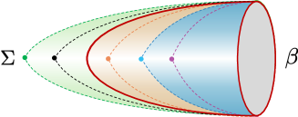
Figure 1: Schematic of the ensemble average for Euclidean Schwarzschild geometries. The orange “cigar” geometry represents the Euclidean Schwarzschild black hole, while the other geometries represented by dashed curves possess conical singularities at their tips. We propose that all the physical quantities should be ensemble-averaged over those geometries, weighted by the corresponding gravitational action.

To address the above problem, we will introduce a method called ensemble average. In this method, all physical quantities are ensemble averaged over different geometries, as displayed in Fig. 1 for Euclidean Schwarzschild geometries. Let us assume the corresponding Hawking temperature of the Schwarzschild black hole is $T_{\text{H}}=1/\beta_{\text{H}}$. When the periodicity of Euclidean time deviates from $\beta_{\text{H}}$, a conical singularity will occur. In the Euclidean path integral for quantum gravity, all possible geometries including those with $\beta\neq\beta_{\text{H}}$, should be included in and weighted by the action. Moreover, physical quantities related to the Schwarzschild metric should be an ensemble average over all the geometries, because all the geometries shown in Fig. 1 are described by the same Lorentzian metric. When an ensemble average over all the above geometries is introduced, we would see that many intriguing properties naturally arise.

There are further motivations for introducing ensemble average from low-dimensional gravity, where the concept was introduced to understand the factorization puzzle Saad2019 ; AfkhamiJeddi2020 ; Maloney2020 ; Penington2019a ; Marolf2020a ; Maldacena2016a ; Jensen2016 ; Heckman:2021vzx ; Cheng:2022nra ; Jafferis:2024jkb . It was proposed that wormholes can be understood as the variance of the averaging, such that factorization is not a necessary property both in the bulk and boundary. If one is looking for a one-to-one correspondence between the bulk and boundary, the bulk gravity should also be regarded as an ensemble average.

In this letter, we aim to understand black hole physics by introducing the concept of the ensemble average over all geometries on the free energy landscape, and by studying the effects deviating from the classical saddles in the gravitational path integral. The semi-classical limit of the ensemble-averaged physics is just the black hole thermodynamics, where we have the Hawking-Page and small-large black hole phase transitions. The new frame allows us to analyze the quantum gravitational corrections to black hole physics. We study the subleading orders of $G_{\text{N}}$ expansions of the Schwarzschild-AdS and Reissner-Nordström (RN)-AdS black hole, from which we can see the universal structures of the quantum corrections.

II Black hole thermodynamics and ensemble average

The Schwarzschild black hole in asymptotic AdS spacetime is regarded as a thermodynamical system. The temperature $T_{\text{H}}$, entropy $S$ and free energy $F$ of the system can be expressed as Bardeen:1973gs ; Bekenstein:1973ur ; Hawking:1975vcx ; Hawking:1976de

$$T_{\text{H}} = \frac{1}{4\pi r_{\text{H}}}\left(1+\frac{3r_{\text{H}}^{2}}{L^{2}}\right)\,,~{}~{}~{}~{}S=\frac{\pi r_{\text{H}}^{2}}{G_{\text{N}}}\,,$$ (1)

$$F = M-T_{\text{H}}S=\frac{r_{\text{H}}}{4G_{\text{N}}}\left(1-\frac{r_{\text{H}}^{2}}{L^{2}}\right)\,.$$ (2)

$M$ is the mass of the black hole, $r_{\text{H}}$ is the black hole horizon radius, and $L$ is the AdS radius. When the system is regarded as thermodynamical, a state with lower free energy is thermodynamically preferred. So, there is a phase transition between the thermal AdS and black holes at Hawking-Page temperature $T_{\text{HP}}$. The transition is called the Hawking-Page transition. In black hole thermodynamics, varying $G_{\text{N}}$ does not influence the phase diagram, because only saddle points are considered, and $G_{\text{N}}$ has no contributing effect.

In the path integral approach to a quantum theory of gravity, one should integrate over all possible geometries weighted by action $S[g]$. The partition function can be evaluated via Euclidean path integral, with Euclidean geometries and Euclidean action $I_{\text{E}}[g]$ Gibbons:1976ue . Since all the geometries shown in Fig. 1 are described by the same Lorentz metric, which is a solution of Einstein’s equation, they should be included in the path integral. The question now lies on what are their corresponding actions.

Euclidean geometries with conical singularities at their tips were discussed in Fursaev:1995ef ; Solodukhin:1994yz ; Mann:1996bi ; Solodukhin:2011gn ; Li:2022oup . For the Euclidean Schwarzschild-AdS case, the Euclidean Einstein-Hilbert action is given by

$$I_{\text{E}}=-\frac{1}{16\pi G_{\text{N}}}\int_{\mathcal{M}}\left(R+\frac{6}{L^{2}}\right)\sqrt{g}~{}\text{d}^{4}x\,.$$ (3)

When considering a geometry with a conical singularity $\Sigma$ as shown in Fig. 1, the action contains an extra contribution from the conical singularity

$$I_{\Sigma}=-\left(1-\frac{\beta}{\beta_{\text{h}}}\right)\frac{\pi r_{\text{h}}^{2}}{G_{\text{N}}}\,.$$ (4)

$r_{\text{h}}$ is the horizon radius corresponding to the horizon temperature $1/\beta_{\text{h}}$. After the regularization procedure, the final Euclidean action can be evaluated as Li:2022oup

$$I_{\text{E}}[\text{S-AdS}]=\frac{\beta r_{\text{h}}}{2G_{\text{N}}}\left(1+\frac{r_{\text{h}}^{2}}{L^{2}}-2\pi r_{\text{h}}T\right)\,.$$ (5)

Note that as can be seen from (4), when the ensemble temperature equals the horizon temperature, i.e. $\beta=\beta_{\text{h}}$, the extra term vanishes, and we get the Euclidean action of the black hole. So the actions for geometries without conical singularity are also calculated.

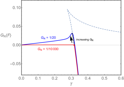
(a) Averaged free energy for the Schwarzschild-AdS spacetime.

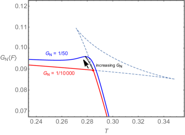
(b) Averaged free energy for the RN-AdS spacetime.

Figure 2: Averaged free energy $\left<{F}\right>$ for the Schwarzschild-AdS and RN-AdS spacetimes. (a) Averaged free energy for the Schwarzschild-AdS spacetime. The blue and red curves represent $\left<{F}\right>$ with $G_{\text{N}}=1/20$ and $G_{\text{N}}=1/10000$. (b) Averaged free energy for the RN-AdS spacetime. The blue and red curves represent the situation with $G_{\text{N}}=1/50$ and $G_{\text{N}}=1/10000$. The Hawking-Page transition and small-large black hole transitions can be regarded as a small $G_{\text{N}}$ approximation of the ensemble-averaged physics, illustrated by the red curves. While for relatively large $G_{\text{N}}$, we do not have a sharp phase transition. The $G_{\text{N}}$ dependence of transition points is indicated by the arrows.

With the Euclidean action, we must include all those geometries with weight $e^{-I_{\text{E}}}$ in the path integral. Moreover, for any physical quantity associated with a certain Lorentzain metric, we should define it as an ensemble-averaged quantity over all the possible Euclidean geometries shown in Fig. 1. The basic principle for defining the ensemble average is that we fix boundary ensemble temperature $T=1/\beta$ and average over the bulk geometries with the same Lorentzian metric but with different horizon temperatures. The ensemble average must be based on the canonical coordinate and conjugate momentum. However, the Euclidean action in (5) is a potential, and we need to consider the perturbative kinetic energy on the potential to determine what variables to integrate in the ensemble average. From Li:2021vdp ; Li:2022yti ; Li:2022ylz , the conjugate momentum is $\dot{r}_{\text{h}}$ and it is natural to use $r_{\text{h}}$ as the canonical coordinate. Integrating over $\dot{r}_{\text{h}}$ results in a constant, which is canceled by the same factor from the denominator. So, we can use $r_{\text{h}}$ to characterize different geometries, and define ensemble-averaged quantity $\left<{A}\right>$ as

$$\left<{A}\right>=\frac{\int A(r_{\text{h}})~{}e^{-I_{\text{E}}(r_{\text{h}})}\text{d}r_{\text{h}}}{\int e^{-I_{\text{E}}(r_{\text{h}})}\text{d}r_{\text{h}}}\,.$$ (6)

For example, the free energy corresponding to the Schwarzschild metric should be an ensemble-averaged quantity

$$\left<{F}\right>=\frac{\int\frac{r_{\text{h}}}{2G_{\text{N}}}\left(1+\frac{r_{\text{h}}^{2}}{L^{2}}-2\pi r_{\text{h}}T\right)~{}e^{-I_{\text{E}}}\text{d}r_{\text{h}}}{\int e^{-I_{\text{E}}}\text{d}r_{\text{h}}}\,.$$ (7)

The ensemble average inherits the spirit of including all the possible geometries in the path integral. $e^{-I_{\text{E}}}$ can be regarded as the probability of each geometry, and $\int e^{-I_{\text{E}}}\text{d}r_{\text{h}}$ in the denominator of (7) is the normalization factor.

The Euclidean action for the RN-AdS case can be derived through a similar method Li:2022oup

$$I_{\text{E}}[\text{RN-AdS}]=\frac{\beta r_{\text{h}}}{2G_{\text{N}}}\left(1+\frac{r_{\text{h}}^{2}}{L^{2}}+\frac{Q^{2}}{r_{\text{h}}^{2}}-2\pi r_{\text{h}}T\right)\,$$ (8)

with the event horizon radius $r_{\text{h}}$. All the physical quantities related to the RN-AdS metric should also be defined as ensemble-averaged ones over all the Euclidean geometries with or without conical singularities.

III Black hole phase transition as a small $G_{\text{N}}$ effect

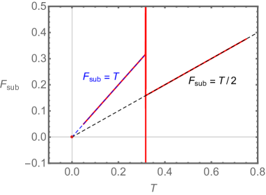
(a) The Schwarzschild-AdS case.

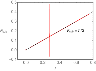
(b) The RN-AdS case.

Figure 3: Subleading-order contributions of the Schwarzschild-AdS and RN-AdS spacetimes. (a) The subleading contribution of the thermal AdS matches $F_{\text{sub}}=T$ shown by the blue dashed line. While the subleading contribution of the Schwarzschild-AdS is $F_{\text{sub}}=T/2$. (b) Before or after the phase transition, the subleading contribution of the RN-AdS is always $F_{\text{sub}}=T/2$.

The Euclidean action for the Schwarzschild-AdS black hole can be rewritten as

$$I_{\text{E}}[\text{S-AdS}]=\frac{\beta r_{\text{h}}}{2l_{\text{pl}}^{2}}\left(1+\frac{r_{\text{h}}^{2}}{L^{2}}-2\pi r_{\text{h}}T\right)\,.$$ (9)

Inspired by the holographic dictionary where the bulk semi-classical limit is defined as small $l_{\text{pl}}^{d-2}/L^{d-2}$ limit, we can use the AdS radius $L$ as the unit length scale and define the dimensionless Newton’s constant $\tilde{G}_{\text{N}}$ as

$$\tilde{G}_{\text{N}}=l_{\text{pl}}^{2}/L^{2}\,.$$ (10)

Then, the Euclidean action (9) can be written as

$$I_{\text{E}}[\text{S-AdS}]=\frac{1}{2\tilde{G}_{\text{N}}}\frac{\beta r_{\text{h}}}{L^{2}}\left(1+\frac{r_{\text{h}}^{2}}{L^{2}}-2\pi r_{\text{h}}T\right)\,.$$ (11)

The so-called semi-classical regime is the situation when $\tilde{G}_{\text{N}}\ll 1$, which also means $l_{\text{pl}}^{2}\ll L^{2}$. For large $\tilde{G}_{\text{N}}$, quantum corrections should be included. From now on, we will drop the tilde sign and regard $G_{\text{N}}\ll 1$ as the semi-classical limit. Whenever considering quantum gravitational corrections, we should be able to recover the black hole thermodynamics in the semi-classical limit. In this section, we will analyze the semi-classical limit of the ensemble-averaged theory and study the deviation from the thermodynamics due to the effects of non-saddle geometries.

The averaged free energies $\left<{F}\right>$ for the Schwarzschild-AdS and RN-AdS spacetimes with varying $G_{\text{N}}$ values are plotted against the ensemble temperature $T$ in Fig. 2a and Fig. 2b, respectively. As indicated by the red curves, the Hawking-Page transition between thermal AdS and a large black hole for Schwarzschild-AdS, and the small-large black hole transition for RN-AdS naturally arise as a result of the small $G_{\text{N}}$ limit. In black hole thermodynamics, the phase transition is a switch of dominant saddles in the Euclidean path integral. The small $G_{\text{N}}$ limit implies the effects away from the saddles can be ignored and we only have a summation of isolated saddles.

Note that for small $G_{\text{N}}$, the thermal AdS geometry naturally arises. This is much less artificial than the Schwarzschild black hole thermodynamics reviewed at the beginning of the previous section, where one needs to separately evaluate and compare the free energy for the thermal AdS and black hole. While the phase transitions naturally arise in the small $G_{\text{N}}$ limit in our case.

While for relatively large $G_{\text{N}}$, there can be non-ignorable contributions from the Euclidean geometries with conical singularities. The non-black-hole geometries included according to the probability $e^{-I_{\text{E}}}$ would have significant influences on black hole physics, and the effect is demonstrated by the deviation of the averaged free energy from the black hole free energy. As can be seen from the blue curves in Fig. 2, the averaged free energy does not exactly match the black hole free energy, and we do not have sharp phase transitions. This phenomenon makes sense in the context of holography duality because finite $1/G_{\text{N}}$ corresponds to finite $N$ in the boundary theory. There would not be a sharp phase transition for a system with finite degrees of freedom. The point with maximal averaged free energy can be more or less regarded as a “transition point” for different phases, because the free energy, after initially increasing, begins to decrease after the point. The transition points for different $G_{\text{N}}$ are illustrated by black dots in Fig. 2 both for the Schwarzschild-AdS and RN-AdS cases. With increasing $G_{\text{N}}$ the trends of the deviations are indicated by black arrows in the figures.

We have some comments on the relation between the ensemble-averaged theory and the black hole free energy landscape. In the free energy landscape proposal Li:2020khm ; Li:2020nsy ; Li:2020spm ; Yang:2021ljn , the topography of the generalized free energy is used to understand the black hole phase transition. Local minimums of the generalized free energy have probabilities of switching to a global one. When this happens, there would be a phase transition. Moreover, the process is understood as stochastic motions in the topographic map and described by the stochastic Fokker-Planck equation. The ensemble-averaged theory proposed here is inspired by the free energy landscape, and we suggest all the geometry (the whole topographic map) should be integrated over with the probability inherited from the gravitational path integral. This provides a natural explanation of the topography and probability in terms of the Euclidean path integral. The free energy landscape is also helpful in understanding our results. For small $G_{\text{N}}$, the valley of the landscape is super deep. The deepness of the global minimum is presented by the crest of the probability $e^{-I_{\text{E}}}$. Thus, we can only see the contribution from the global minimum. As will be seen in the next section, to see the quantum corrections to the black hole thermodynamics one can expand the Euclidean action and the averaged free energy around classical saddles.

IV Non-classical corrections to black hole thermodynamics

To further understand the quantum effects due to the new geometries, we can do the semi-classical expansion of the averaged free energy (7). There are difficulties when directly expanding $G_{\text{N}}$. So we choose to expand around the classical saddle which is the global minimum of the generalized free energy. When the horizon temperature equals the ensemble temperature, we have a bulk black hole without conical singularity whose horizon radius is denoted as $r_{\text{H}}$. Note that $r_{\text{H}}$ means the horizon radius of the “Hawking saddle” Penington2019a , while $r_{\text{h}}$ is a free parameter. We are going to expand $I_{\text{E}}$ up to the second order of $\Delta=r_{\text{h}}-r_{\text{H}}$ near $r_{\text{h}}=r_{\text{H}}$, and integrate over the neighborhood of $r_{\text{H}}$ in (7). Expanding $I_{\text{E}}$ gives us a Gaussian distribution of different geometries. The second-order term corresponds to the $\mathcal{O}(G_{\text{N}}^{0})$ contribution in the averaged free energy. For small $G_{\text{N}}$, the probability distribution $e^{-I_{\text{E}}}$ is very steep near the saddle point, and the Gaussian integral can run from $(r_{\text{H}}-5\sigma,r_{\text{H}}+5\sigma)$ with variance $\sigma^{2}\propto G_{\text{N}}$. The error function of the Gaussian integral can be evaluated, which would be very small.

Expanding the Euclidean action and the free energy to the second order, we have

$$I_{\text{E}}^{\Delta} = \frac{\beta r_{\text{H}}}{2G_{\text{N}}}\left(1+\frac{r_{\text{H}}^{2}}{L^{2}}-2\pi r_{\text{H}}T\right)+\frac{3\beta r_{\text{H}}-2\pi L^{2}}{2G_{\text{N}}L^{2}}\Delta^{2}\,,$$

$$F^{\Delta} = \frac{r_{\text{H}}}{2G_{\text{N}}}\left(1+\frac{r_{\text{H}}^{2}}{L^{2}}-2\pi r_{\text{H}}T\right)+\frac{3r_{\text{H}}-2\pi L^{2}T}{2G_{\text{N}}L^{2}}\Delta^{2}\,.$$

The coefficient of the $\Delta^{2}$ term can be identified as $1/(2\sigma^{2})$. Then the averaged free energy can be evaluated as

$$\left<{F}\right> \approx \frac{\int_{-5\sigma}^{+5\sigma}F^{\Delta}e^{-I_{\text{E}}^{\Delta}}\text{d}\Delta}{\int_{-5\sigma}^{+5\sigma}e^{-I_{\text{E}}^{\Delta}}\text{d}\Delta}$$ (12)

$$= \frac{r_{\text{H}}}{4G_{\text{N}}}\left(1-\frac{r_{\text{H}}^{2}}{L^{2}}\right)+\frac{T}{2}+\frac{5e^{-\frac{25}{2}}}{\sqrt{2\pi}~{}\text{erf}\left(\frac{5}{\sqrt{2}}\right)}T.$$

As expected, the leading-order contribution is just the black hole free energy shown in (2). The subleading contribution of order $\mathcal{O}(G_{\text{N}}^{0})$ can be approximated as $F_{\text{sub}}^{\text{BH}}=T/2$. The last error term due to integrating over $(-5\sigma,5\sigma)$ in (12) is $7.4\times 10^{-6}\times T$, thus can be ignored. The subleading-order contribution for the RN-AdS case can be derived by a similar method, and we also have $F_{\text{sub}}^{\text{BH}}=T/2$. Note that we expand the free energy near the saddle point, where the ensemble temperature $T$ should be approximate to the Hawking temperature $T_{\text{H}}$ due to small $\sigma\propto G_{\text{N}}$ for small $G_{\text{N}}$. So we have a corrected free energy with subleading correction roughly equals $T_{\text{H}}/2$.

Let us consider the thermal AdS case which can be regarded as the zero $r_{\text{h}}$ limit of the Schwarzschild-AdS black hole. With a deformation $\Delta$, the Euclidean action and free energy can be denoted as

$$I_{\text{E}}^{\Delta}=\frac{\beta\Delta}{2G_{\text{N}}}\,,~{}~{}~{}~{}F^{\Delta}=\frac{\Delta}{2G_{\text{N}}}\,.$$ (13)

The averaged free energy can be calculated near the AdS saddle as

$$\left<{F}\right>\approx\frac{\int_{0}^{5\sqrt{G_{\text{N}}}}F^{\Delta}~{}e^{-I^{\Delta}_{\text{E}}}\text{d}\Delta}{\int_{0}^{5\sqrt{G_{\text{N}}}}e^{-I^{\Delta}_{\text{E}}}\text{d}\Delta}=T\,.$$ (14)

The error term can always be ignored because $\beta\gg\sqrt{G_{\text{N}}}$ always guarantees the error is super small. So for the thermal AdS case, the $1/G_{\text{N}}$-order contribution is zero, and the subleading contribution can be derived as $F_{\text{sub}}^{\text{AdS}}=T$.

From the above calculation, the subleading-order contribution of $G_{\text{N}}$ can be derived by expanding around the classical saddle, which can be verified by numerical demonstration of the leading and subleading-order contributions. Figure 3 illustrates the numerical result of the subleading free energies of the Schwarzschild-AdS and RN-AdS spacetimes. As can be seen from the figures, away from the choppy transition points, the subleading contributions of the black holes are exactly $F_{\text{sub}}=T/2$ for both the Schwarzschild-AdS and RN-AdS black holes. There must be some universal structures for the two cases that result in the same subleading-order behavior. Moreover, the thermal AdS phase exactly matches the analytical analysis, which is $F_{\text{sub}}=T$.

The subsubleading-order correction to the black hole free energy can be derived and shown in Fig. 4. Besides the vibration near the transition point, we have different smooth behaviors before and after the transition, which can be fitted as a function of ensemble temperature $T$. The physical free energy should be the summation of those different pieces of the free energies, i.e.

$$\left<{F}\right>=F_{\text{leading}}+F_{\text{sub}}\cdot G_{\text{N}}^{0}+F_{\text{subsub}}\cdot G_{\text{N}}^{1}+\mathcal{O}(G_{\text{N}}^{2})\,,$$ (15)

with the black hole free energy $F_{\text{leading}}\propto 1/G_{\text{N}}$. For small $G_{\text{N}}$, such as $G_{\text{N}}=1/1000$, $\mathcal{O}(G_{\text{N}}^{2})$ terms can be ignored, and keeping the first several terms in (15) is good enough to capture the corrected thermodynamics due to the geometries with conical singularity.

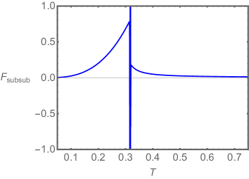
Figure 4: An illustration of the subsubleading-order free energy of the Schwarzschild-AdS spacetime.

V Summary and discussion

In this letter, the action for Euclidean geometries with a conical singularity was calculated, and we argued that in the path integral approach to quantum gravity, all those geometries should be included in the path integral. Because the geometries are described by the same Lorentzian metric, any physical quantity related to the metric should be ensemble-averaged over the Euclidean geometries. Working with averaged quantities, we concluded that the Hawking-Page transition for the Schwarzschild-AdS spacetime and the small-large black hole transition for the RN-AdS spacetime can be directly derived in the semi-classical limit. No extra assumption is needed. The averaged free energy deviates from that of the black hole for relatively large $G_{\text{N}}$. The subleading order of $G_{\text{N}}$ contributions can be reproduced by expanding around the saddle point, which are both $T/2$ for the Schwarzschild and RN black holes. The analytical and numerical results exactly match. Thus, we conjecture that there is a universal structure for black holes and the same result should also hold for other black holes. Beyond the semi-classical limit, we have quantum-corrected black hole thermodynamics, where the subleading contributions can not be ignored and the effects considered here would be important.

We have some further discussions related to the main results. In the Schwarzschild-AdS case, we did not mention the thermal AdS but just evaluated the averaged free energy of the Schwarzschild-AdS metric. It turns out that pure AdS naturally arises and dominates at low temperatures, as can be seen from Fig. 2a. However, for Einstein-Maxwell theory, the thermal AdS is not a solution for non-vanishing $Q$, we would not see such a phase transition between black holes and pure AdS. The Hawking-Page and small-large black hole phase transitions are two types of transitions, but the ensemble average seems clever enough to understand the two types simultaneously.

For the Hawking-Page phase transition, there is a dual large-$N$ SU($N$) description. It is well known that it is a transition between states with free energies scaling with $\mathcal{O}(N^{0})$ and $\mathcal{O}(N^{2})$ in the boundary theory. The thermal AdS spacetime is dual to state with constant free energy and the asymptotic AdS black hole is dual to state with free energy scales as $N^{2}$. The finite $G_{\text{N}}$ effects that deviate from the thermal AdS and black hole, should dual to the boundary finite $N$ physics. One can figure out the subleading terms in large $N$ expansion through the duality between the two sides, which may be able to provide further insights into the boundary theory.

References

- (1) S. W. Hawking and D. N. Page, “Thermodynamics of Black Holes in anti-De Sitter Space,” Commun. Math. Phys. 87 (1983) 577–588.
- (2) E. Witten, “Anti-de Sitter space, thermal phase transition, and confinement in gauge theories,” Adv. Theor. Math. Phys. 2 (1998) 505–532, arXiv:hep-th/9803131.
- (3) D. J. Gross and E. Witten, “Possible Third Order Phase Transition in the Large N Lattice Gauge Theory,” Phys. Rev. D 21 (1980) 446–453.
- (4) B. Sundborg, “The Hagedorn transition, deconfinement and N=4 SYM theory,” Nucl. Phys. B 573 (2000) 349–363, arXiv:hep-th/9908001 [hep-th].
- (5) A. Chamblin, R. Emparan, C. V. Johnson, and R. C. Myers, “Holography, thermodynamics and fluctuations of charged AdS black holes,” Phys. Rev. D 60 (1999) 104026, arXiv:hep-th/9904197.
- (6) A. Chamblin, R. Emparan, C. V. Johnson, and R. C. Myers, “Charged AdS black holes and catastrophic holography,” Phys. Rev. D 60 (1999) 064018, arXiv:hep-th/9902170.
- (7) D. Kastor, S. Ray, and J. Traschen, “Enthalpy and the Mechanics of AdS Black Holes,” Class. Quant. Grav. 26 (2009) 195011, arXiv:0904.2765 [hep-th].
- (8) B. P. Dolan, “Pressure and volume in the first law of black hole thermodynamics,” Class. Quant. Grav. 28 (2011) 235017, arXiv:1106.6260 [gr-qc].
- (9) D. Kubiznak and R. B. Mann, “P-V criticality of charged AdS black holes,” JHEP 07 (2012) 033, arXiv:1205.0559 [hep-th].
- (10) S.-W. Wei and Y.-X. Liu, “Insight into the Microscopic Structure of an AdS Black Hole from a Thermodynamical Phase Transition,” Phys. Rev. Lett. 115 (2015) 111302, arXiv:1502.00386 [gr-qc]. [Erratum: Phys.Rev.Lett. 116, 169903 (2016)].
- (11) R. Li and J. Wang, “Thermodynamics and kinetics of Hawking-Page phase transition,” Phys. Rev. D 102 (2020) 024085.
- (12) R. Li, K. Zhang, and J. Wang, “Thermal dynamic phase transition of Reissner-Nordström Anti-de Sitter black holes on free energy landscape,” JHEP 10 (2020) 090, arXiv:2008.00495 [hep-th].
- (13) R. Li and J. Wang, “Energy and entropy compensation, phase transition and kinetics of four-dimensional charged Gauss-Bonnet Anti-de Sitter black holes on the underlying free energy landscape,” Nucl. Phys. B 976 (2022) 115714, arXiv:2012.05424 [gr-qc].
- (14) S.-J. Yang, R. Zhou, S.-W. Wei, and Y.-X. Liu, “Kinetics of a phase transition for a Kerr-AdS black hole on the free-energy landscape,” Phys. Rev. D 105 (2022) 084030, arXiv:2105.00491 [gr-qc].
- (15) R. Li, K. Zhang and J. Wang, “Probing black hole microstructure with the kinetic turnover of phase transition,” Phys. Rev. D 104 (2021) 084076, arXiv:2102.09439 [gr-qc].
- (16) R. Li and J. Wang, “Non-Markovian dynamics of black hole phase transition,” Phys. Rev. D 106 (2022) 104039, arXiv:2205.00594 [gr-qc].
- (17) R. Li and J. Wang, “Kinetics of Hawking-Page phase transition with the non-Markovian effects,” JHEP 05 (2022) 128, arXiv:2201.06138 [gr-qc].
- (18) P. Saad, S. H. Shenker, and D. Stanford, “JT gravity as a matrix integral,” arXiv:1903.11115 [hep-th].
- (19) N. Afkhami-Jeddi, H. Cohn, T. Hartman, and A. Tajdini, “Free partition functions and an averaged holographic duality,” JHEP 01 (2021) 130, arXiv:2006.04839 [hep-th].
- (20) A. Maloney and E. Witten, “Averaging Over Narain Moduli Space,” JHEP 10 (2020) 187, arXiv:2006.04855 [hep-th].
- (21) G. Penington, S. H. Shenker, D. Stanford, and Z. Yang, “Replica wormholes and the black hole interior,” JHEP 03 (2022) 205, arXiv:1911.11977v2.
- (22) D. Marolf and H. Maxfield, “Transcending the ensemble: baby universes, spacetime wormholes, and the order and disorder of black hole information,” JHEP 08 (2020) 044, arXiv:2002.08950.
- (23) J. Maldacena and D. Stanford, “Comments on the Sachdev-Ye-Kitaev model,” Phys. Rev. D 94 (2016) 106002 , arXiv:1604.07818 [hep-th].
- (24) K. Jensen, “Chaos in AdS2 holography,” Phys. Rev. Lett. 117 (2016) 111601, arXiv:1605.06098 [hep-th].
- (25) J. J. Heckman, A. P. Turner, and X. Yu, “Disorder averaging and its UV discontents,” Phys. Rev. D 105 (2022) 086021, arXiv:2111.06404 [hep-th].
- (26) P. Cheng and P. Mao, “Notes on Wormhole Cancellation and Factorization,” Eur. Phys. J. C 84 (2024) 675, arXiv:2208.08456 [hep-th].
- (27) D. L. Jafferis, L. Rozenberg and G. Wong, “3d Gravity as a random ensemble,” arXiv:2407.02649 [hep-th].
- (28) J. M. Bardeen, B. Carter, and S. W. Hawking, “The four laws of black hole mechanics,” Commun. Math. Phys. 31 (1973) 161–170.
- (29) J. D. Bekenstein, “Black holes and entropy,” Phys. Rev. D 7 (1973) 2333–2346.
- (30) S. W. Hawking, “Particle Creation by Black Holes,” Commun. Math. Phys. 43 (1975) 199–220. [Erratum: Commun.Math.Phys. 46, 206 (1976)].
- (31) S. W. Hawking, “Black Holes and Thermodynamics,” Phys. Rev. D 13 (1976) 191–197.
- (32) G. W. Gibbons and S. W. Hawking, “Action Integrals and Partition Functions in Quantum Gravity,” Phys. Rev. D 15 (1977) 2752–2756.
- (33) D. V. Fursaev and S. N. Solodukhin, “On the description of the Riemannian geometry in the presence of conical defects,” Phys. Rev. D 52 (1995) 2133–2143, arXiv:hep-th/9501127.
- (34) S. N. Solodukhin, “The Conical singularity and quantum corrections to entropy of black hole,” Phys. Rev. D 51 (1995) 609–617, arXiv:hep-th/9407001.
- (35) R. B. Mann and S. N. Solodukhin, “Conical geometry and quantum entropy of a charged Kerr black hole,” Phys. Rev. D 54 (1996) 3932–3940, arXiv:hep-th/9604118.
- (36) S. N. Solodukhin, “Entanglement entropy of black holes,” Living Rev. Rel. 14 (2011) 8, arXiv:1104.3712 [hep-th].
- (37) R. Li and J. wang, “Generalized free energy landscape of a black hole phase transition,” Phys. Rev. D 106 (2022) 106015, arXiv:2206.02623 [hep-th].