Leveraging Invariant Principle for Heterophilic Graph Structure Distribution Shifts

Abstract

Heterophilic Graph Neural Networks (HGNNs) have shown promising results for semi-supervised learning tasks on graphs. Notably, most real-world heterophilic graphs are composed of a mixture of nodes with different neighbor patterns, exhibiting local node-level homophilic and heterophilic structures. However, existing works are only devoted to designing better HGNN backbones or architectures for node classification tasks on heterophilic and homophilic graph benchmarks simultaneously, and their analyses of HGNN performance with respect to nodes are only based on the determined data distribution without exploring the effect caused by this structural difference between training and testing nodes. How to learn invariant node representations on heterophilic graphs to handle this structure difference or distribution shifts remains unexplored. In this paper, we first discuss the limitations of previous graph-based invariant learning methods from the perspective of data augmentation. Then, we propose HEI, a framework capable of generating invariant node representations through incorporating heterophily information to infer latent environments without augmentation, which are then used for invariant prediction, under heterophilic graph structure distribution shifts. We theoretically show that our proposed method can achieve guaranteed performance under heterophilic graph structure distribution shifts. Extensive experiments on various benchmarks and backbones can also demonstrate the effectiveness of our method compared with existing state-of-the-art baselines.

1 Introduction

Graph Neural Networks (GNNs) have emerged as prominent approaches for learning graph-structured representations through the aggregation mechanism that effectively combines feature information from neighboring nodes chen2021pareto ; zheng2022graph ; chen2024learning ; chen2024pareto . Previous GNNs primarily dealt with homophilic graphs, where connected nodes tend to share similar features and labels zhu2020beyond . However, growing empirical evidence suggests that these GNNs’ performance significantly deteriorates when dealing with heterophilic graphs, where the majority of nodes connect with others from different classes, even worse than the traditional neural networks lim2021large . An appealing way to address this issue is to tailor the heterophily property to GNNs, extending the range of neighborhood aggregation and reorganizing architecture zheng2022graph , known as the heterophilic GNNs (HGNNs).

Heterophilic Graph Structure distribution Shift(HGSS): A novel data distribution shift perspective to reconsider existing HGNNs works. Despite promising, most previous HGNNs assume the nodes share the determined data distribution lim2021large ; li2022finding , we argue that there is data distribution disparity among nodes with different labels. As illustrated in Figure 1(a1), heterophilic graphs are composed of a mixture of nodes that exhibit local homophilic and heterophilic structures, i.e, the nodes have different neighbor patterns . Here, we identify their varying neighbor patterns between train and test nodes as the Heterophilic Graph Structure distribution Shift (Figure 1(a2)). This kind of shift was neglected by previous works and truly affected GNN’s performance. As shown in Figure 1(a3), we visualize the HGSS between training and testing nodes on the Squirrel dataset. Compared with test nodes, the train nodes are more prone to be categorized into groups with high homophily, which may yield a test performance degradation. More statistical results on other heterophilic graph datasets can be shown in the Appendix A.4. Notably, we acknowledge that some work mao2023demystifying also discusses homophilic and heterophilic structural patterns, but until now they don’t provide a clear technique solution for this problem. Exactly, apart from mao2023demystifying , our work is orthogonal to most HGNNs works zheng2022graph that focus on designing backbones or architectures without considering the HGSS issue. Thus, it’s extremely urgent to seek solutions from the perspective of data distribution to address the HGSS in the context of node-level tasks within heterophilic graphs.

Existing graph-based invariant learning methods perform badly for HGSS due to the environments construction strategy. In the context of general distribution shifts, the technique of invariant learning rong2019dropedge is increasingly recognized for its efficacy in mitigating these shifts. The foundational approach involves learning node representations to facilitate invariant predictor learning across various constructed environments (Figure 1(b1)), adhering to the Risk Extrapolation (REx) principle wu2022handling ; chen2022ba ; liu2023flood .

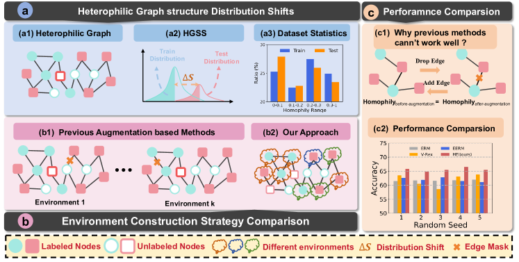
Figure 1: (a) illustrates the heterophilic graph structure distribution shifts (HGSS), where the figure and histogram show the HGSS and neighbor pattern (measured by node homophily) difference between train and test nodes on the Squirrel dataset; (b) displays the comparison of different environment construction strategies between previous works and ours, the key exists that we don’t need to construct environments with augmentation; (c) shows that previous environment construction strategy may be ineffective in addressing our defined HGSS due to the unchanged neighbor pattern distribution. The experimental results can provide support for our analysis and verify that our proposed HEI can consistently outperform other baselines.

Unfortunately, previous graph-based invariant learning methods may not effectively address heterophilic graph structure distribution shifts, primarily due to explicit environments that may be ineffective for invariant learning. As illustrated in Figure 1(c1), within HGSS settings, altering the original structure does not consistently affect the node’s neighbor patterns. In essence, obtaining optimal and varied environments pertinent to neighbor patterns is challenging. Our observation (Figure 1(c2)) reveals that EERM wu2022handling , a pioneering invariant learning approach utilizing environment augmentation to tackle graph distribution shifts in node-level tasks, does not perform well under HGSS settings. At times, its enhancements are less effective than simply employing the original V-Rex krueger2021out , which involves randomly distributing the train nodes across various environmental groups. We attribute this phenomenon to the irrational environment construction. According to our analysis, EERM is essentially a node environment-augmented version of V-Rex, i.e., the disparity in their performance is solely influenced by the differing strategies in environmental construction. Besides, from the perspective of theory assumption, V-Rex is initially employed to aid model training by calculating the variance of risks introduced by different environments as a form of regularization. The significant improvements by V-Rex also reveal that the nodes of a single input heterophilic graph may reside in distinct environments, considering the variation in neighbor patterns, thus contradicting EERM’s prior assumption that all nodes in a graph share the same environment wu2022handling . Based on this insight, our goal is to break away from previous explicit environment augmentation to learn the latent environment partition, which empowers the invariant learning to address the HGSS better.

HEI: A Heterophil-inspired Environment inference framework for invariant prediction. Recent findings confirm that obtaining an accurate environment partition without prior knowledge is unfeasible  lin2022zin . Therefore, our initial step should be to quantify the nodes’ neighbor pattern properties related to the HGSS, which are central to the issue at hand. Consequently, a critical question emerges: During the training phase, how can we identify an appropriate metric to estimate the node’s neighbor pattern and leverage it to deduce latent environments to manage this HGSS issue? As previously mentioned, node homophily or edge homophily can assess neighbor patterns for dataset description lim2021large . Unfortunately, this requires the actual labels of the node and its neighbors, rendering it inapplicable during the training stage due to the potential unlabeled status of neighbor nodes. To cope with this problem, several evaluation metrics pertinent to nodes’ neighbor patterns, including local similarity chen2023lsgnn , post-aggregation similarity luan2022revisiting , and SimRank liu2023simga , have been introduced. These metrics aim to facilitate node representation learning on heterophilic graphs during the training phase. However, while these studies primarily concentrate on employing these metrics to enhance neighbor aggregation for improved HGNN architectures, our objective is to introduce framework-agnostic backbones, augmented by estimated neighbor pattern insights, to tackle distribution shifts. A thorough analysis is essential to evaluate these metrics’ efficacy as dependable indicators of the node’s environments, both from causal and graph-theoretical perspectives. Therefore, we propose HEI, a framework capable of generating invariant node representations through incorporating heterophily information to inference latent environments,as shown in Figure 1 (b2), which are then used for downstream invariant prediction, under heterophilic graph structure distribution shifts. Moreover, we adapt this framework to the latest SOTA HGNN backbones to further verify its orthogonality to previous HGNN works. Simultaneously, the comparison experiments with previous methods designed for mitigating agnostic distribution shifts on various graph benchmarks can verify its effectiveness in addressing this neglected HGSS issue.

Our Contributions:(i) We highlight an important yet often neglected form of heterophilic graph structure distribution shift, which is orthogonal to most HGNN works that focus on backbone designs;(ii) We propose HEI, a novel graph-based invariant learning framework to tackle the HGSS issue. Unlike previous efforts, our method emphasizes leveraging a node’s inherent heterophily information to deduce latent environments without augmentation, thereby significantly improving the generalization and performance of HGNNs;(iii) We demonstrate the effectiveness of our proposed method on several benchmarks and backbones compared with existing methods.

2 Preliminaries

Notations. Given an input graph $G=(V,X,A)$, we denote $V\in\{v_{1},...,v_{N}\}$ as the nodes set, $X\in R^{N\times D}$ as node features and $A\in\{0,1\}^{N\times N}$ as an adjacency matrix representing whether the nodes connect, where the $N$ and $D$ denote the number of nodes and features, respectively. The node labels can be defined as $Y\in\{0,1\}^{N\times C}$, where C represents the number of classes. For each node $v$, we use $A_{v}$ and $X_{v}$ to represent its adjacency matrix and node feature.

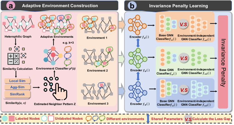
Figure 2: Illustrations of our framework HEI. (a) The neighbor pattern for each train node can be estimated by similarity first and then used for inferring environments without augmentation; (b) Based on the train nodes belonging to different inferred environments, we can train a set of environment-independent GNN classifiers with the shared encoder compared with the base GNN. The shared encoder outputs the representations of nodes in each environment and then forwards them to the base GNN classifier and the environment-independent classifier respectively. By calculating the loss gap between these two different classifiers, an invariance penalty is introduced to improve model generalization.

Problem Formulation. We provide the formulation for the node-level OOD problems on graphs. From the perspective of data generation, we can get train data $\left(G_{train},Y_{train}\right)$ from train distribution $p(\mathbf{G,Y})|\mathbf{e}=e)$, the model should handle the test data $\left(G_{test},Y_{test}\right)$ from a different distribution $p(\mathbf{G,Y})|\mathbf{e}=e^{\prime})$. Considering the specific neighbor aggregation process, the general optimized object of node-level OOD problem on graphs can be formulated as follows:

$$\min_{\omega,\Phi}\max_{e\in\mathcal{E}}\mathbb{E}_{G}\frac{1}{N}\sum_{v\in V}\mathbb{E}_{y\sim p(\mathbf{y}|\mathbf{A}_{\mathbf{v}}=A_{v},\mathbf{X}_{\mathbf{v}}=X_{v},\mathbf{e}=e)}l(f_{\omega}\left(f_{\Phi}\left(A_{v},X_{v}\right)\right),y_{v})$$ (1)

where the $\mathcal{E}$ represents the support of environments, the $f_{\omega}$ and $f_{\Phi}$ refer to GNN’s classifier and feature extractor respectively and $l(\cdot)$ is a loss function(e.g. cross entropy). The Equation 1 aims to learn a robust model that minimizes loss across environments as much as possible. Only in this way, can the trained model be likely to adapt to unknown target test distribution well. However, environmental labels for nodes are usually unavailable during the training stage, which inspires many works to seek methods to make use of environmental information to help model training.

Previous Graph-based Invariant Learning. To approximate the optimized object of Eq. 1, previous works wu2022handling ; chen2022ba ; liu2023flood mainly construct diverse environments by adopting the masking strategy as Figure 1(b1). Thus, we conclude previous works from the mask strategy. Denote the masking strategy as $Mask_{\eta}(\cdot)$ parameterized with $\eta$, given an input single graph, we can obtain K augmented graphs as Eq. 2, where each graph corresponds to an environment. The K is a pre-defined number of training environments.

$$G^{e=k}=Mask^{e=k}_{\eta}(G)=\left(X^{m},A^{m},V^{m}\right)_{e=k},k=1,2...,K$$ (2)

Then, assisted by these augmented graphs with environment label, the GNN $f(\cdot)$ parameterized by $\left(\omega,\Phi\right)$ can be trained considering environmental information. We can define the ERM loss in the $k$-th environment as the Eq.3, which only calculates the loss on the corresponding augmented $G^{e=k}$.

$$R_{e=k}\left(\omega,\Phi\right)=\frac{1}{N}\sum_{v\in V^{m}}l\left(f_{\omega}(f_{\Phi}\left(A_{v},X_{v}\right),y_{v}\right)$$ (3)

Following the principle of Variance Risk Extrapolation (V-Rex) to reduce the risks from different environments, the final training framework can be defined as Eq. 2. Where the $\lambda$ controls the effect between reducing the average risk and promoting equality of risks.

$$\min_{\omega,\Phi}\max_{\eta}~{}L\left(\Phi,\omega,\eta\right)=$$

$$\sum\nolimits_{k=1}^{K}{R_{e=k}(\omega,\Phi)}+\lambda Var\left(R_{e=1}(\omega,\Phi),\cdots,R_{e=K}(\omega,\Phi)\right)$$ (4)

The maximization means that we should optimize the masking strategy (parameter $\eta$) to construct sufficient and diverse environments, while the minimization aims to minimize the training loss for the model (parameter $\omega$ and $\Phi$).

Discussions. Exactly, previous graph-based invariant learning methods introduce extra augmented graphs to construct nodes’ environments while our work only infers nodes’ environments on a single input graph. Moreover, for previous works, there exists a latent assumption that nodes on a single graph belong to the same environment so we need to construct diverse environments by data augmentation. Exactly, this assumption arises from the insight that nodes on an input graph come from the same outer domain-related environments(e.g. Financial graphs or Molecular graphs)wu2022handling . But considering the message-passing mechanism on heterophilic graphs(the ideal aggregation target should be nodes with the same label), the nodes should exist exactly in inner structure-related environments. Therefore, for the HGSS issue, we should consider seeking new methods to make use of the node’s environmental information for invariant prediction. Or as shown in Figure 1(c1), directly succeeding in utilizing data augmentation may be ineffective in changing the node’s neighbor pattern to construct diverse environments. At the same time, the neighbor pattern difference between train and test has verified that even on a single graph, the nodes may belong to different structure-related environments, which inspires us to directly infer their environments, assisted by the node’s neighbor pattern, for addressing heterophilic graph structure distribution shift.

3 Methodology

In this section, we present the details of the proposed HEI. Firstly, on heterophilic graphs, we verify that the similarity can serve as a neighbor pattern indicator and then review existing similarity-based metrics to estimate the neighbor patterns during training stages. Then, we elaborate the framework to jointly learn environment partition and invariant node representation on heterophilic graphs without augmentation, assisted by the estimated neighbor patterns. Finally, we clarify the overall training process of the algorithm and discuss its complexity. Moreover, we provide a detailed theoretical analysis in Appendix A.3 to clarify the effectiveness of HEI.

3.1 Neighbor Patterns Estimation

The node homophily and edge homophily are commonly used metrics to evaluate the node’s neighbor patterns[20], but unfortunately, both of them need the true labels of the node and its neighbors, which means they can not be used in the training stage because the neighbor nodes may be just the test nodes without labels. To cope with it, we achieve inspiration from previous studies that focus on HGNN’s backbone designs luan2022revisiting ; chen2023lsgnn ; liu2023simga and verify that the neighbor pattern can be estimated by similarity.

Similarity: An Indicator of Neighbor Patterns. Though previous works have shown there may exist somewhat relationship between similarity and homophily from the experimental analysis chen2023lsgnn , it can not be guaranteed to work well without a theory foundation. Thus, we further investigate its effectiveness from the node cluster view and verify the similarity between nodes can be exploited to approximate the neighbor pattern without the involvement of label information. For simplicity, we take K-Means as the cluster algorithm. For two nodes $v$ and $u$, let $v$ belong to the cluster centroid $c_{1}$ and denote the distance between $v$ and $u$ as $\delta=\left\|u-v\right\|^{2}$, where we can get $c_{1}={\arg\min}\left\|v-c_{i}\right\|^{2}$, where $c_{i}$ represent the $i$-th cluster centroid. Then the distance between $u$ and cluster centroid $c_{1}$ can be acquired by the Eq. 9. Exactly, the neighbor pattern describes the label relationship between the node and its neighbors. From the Eq 9, we can find the smaller $\delta$, the more likely the $v$ and $u$ belong to the same cluster and own the same label. Therefore, the similarity between nodes can be exploited to serve as a neighbor pattern indicator without using label information.

$$\begin{array}[]{l}\left\|u-c_{1}\right\|^{2}=\left\|\left(u-v\right)+\left(v-c_{1}\right)\right\|^{2}\\ =\left\|\left(u-v\right)\right\|^{2}+2\left\|u-v\right\|\left\|v-c_{1}\right\|+\left\|v-c_{1}\right\|^{2}\\ =\delta+2\sqrt{\delta}\left\|v-c_{1}\right\|+\left\|v-c_{1}\right\|^{2}\\ =\left(\left\|v-c_{1}\right\|+\sqrt{\delta}\right)^{2}\geq\delta\end{array}$$ (9)

Existing Similarity-based Metrics. Existing similarity-based metrics on heterophilic graphs can be shown as Eq.10.

$$Similarity(u,v)\begin{cases}\operatorname{Sim}(X_{v},X_{u})&,LocalSim\\ \operatorname{Sim}(\hat{A_{v}}X_{v},\hat{A_{u}}X_{u})&,AggSim\\ \frac{c}{|NS(u)||NS(v)|}\sum\limits_{u^{\prime}\in NS(u)\atop v^{\prime}\in NS(v)}\operatorname{Sim}(X_{u^{\prime}},X_{v^{\prime}})&,SimRank\end{cases}$$ (10)

Specifically, the local similarity(Local Sim chen2023lsgnn ), and post-aggregation similarity (Agg-Sim luan2022revisiting ) calculate the similarity of the original feature and post-aggregation embedding between two nodes, respectively. In contrast, the SimRank liu2023simga calculates the similarity between their respective neighbor nodes. The $c\in(0,1)$ is a decay factor empirically set to 0.6, the $NS(v)$ denotes $v$’s neighbor set including the nodes connected to $v$ and the $\hat{A_{v}}$ denotes the aggregation operation on the node $v$.

Estimated Neighbor Patterns. Thus, as shown by the Eq.11, we can obtain the estimated neighbor patterns $z_{v}$ for the node $v$ during the training stage by averaging the node’s similarity with neighbors.

$$z_{v}=\frac{1}{|NS(v)|}\sum_{u\in NS(v)}Similarity(u,v)$$ (11)

Notably, we further strengthen our object of using similarity metrics is indeed different from previous HGNN works that also utilize the similarity metricsluan2022revisiting ; chen2023lsgnn ; liu2023simga . We focus on utilizing the neighbor pattern to infer the node’s environment for invariant prediction(separate and weaken the effect of spurious feature as shown in Figure 9, when given the neighbors). But previous HGNN works mainly aim to help the node select proper neighbors and then directly utilize full neighbor features as aggregation targets for better HGNN backbone designs. Our work is exactly orthogonal to previous HGNN works.

3.2 Our Proposed Invariant Learning Framework

Our work aims to utilize the estimated neighbor patterns $Z\in R^{G_{z}}$ for nodes as auxiliary information to jointly learn nodes’ environment partition and invariant node representation without augmentation. Similar ideas can be also shown in chang2020invariant ; lin2022zin that we can rely on some auxiliary information for invariant prediction without environmental labels,

Specifically, assisted by the estimated neighbor patterns for nodes, we can train an environment classifier $\rho(\cdot):R^{G_{z}}\xrightarrow{}R^{K}$ that softly assigns the train nodes to $K$ environments. The $K$ is a pre-defined number, $\rho$ is a two-layer MLP and the $\rho^{(k)}(\cdot)$ is denoted as the $k$-th entry of $\rho(\cdot)$, with $\rho(Z)\in[0,1]^{K}$ and $\sum_{k}\rho^{(k)}(Z)=1$. Denote the ERM loss as $R(\omega,\Phi)$, which is calculated on all train nodes. Then, as shown in Eq. 12, the ERM loss in the $k$-th inferred environment can be defined as $R_{\rho^{(k)}}(\omega,\Phi)$, which only calculates the loss on the nodes belonging to the $k$-th environment.

$$R_{\rho^{(k)}}(\omega,\Phi)=\frac{1}{N}\sum_{v\in V}\rho^{(k)}(z_{v})l\left(f_{\omega}(f_{\Phi}\left(A_{v},X_{v}\right),y_{v}\right)$$ (12)

Therefore, the training framework can be defined as Eq. 13.

$$\min_{\omega,\Phi}\;\max_{\rho,\{\omega_{1},\cdots,\omega_{K}\}}~{}L(\Phi,\omega,\omega_{1},\cdots,\omega_{K},\rho)=$$

$$R(\omega,\Phi)+\lambda\underbrace{\sum\nolimits_{k=1}^{K}\big{[}R_{\rho^{(k)}}(\omega,\Phi)-R_{\rho^{(k)}}(\omega_{k},\Phi)\big{]}}_{\text{\small invariance penalty}}$$ (13)

Compared with Eq. 3 and Eq. 2, our framework mainly differs in the maximization process. Thus, we clarify the effectiveness of our framework from two aspects: (i) The invariance penalty that introduces a set of environment-dependent GNN classifiers $\{f_{\omega_{k}}\}_{k=1}^{K}$, which are only trained on the data belonging to the inferred environments; (ii) The optimization of environmental classifier $\rho(\cdot)$;

Invariance Penalty Learning. As shown by Eq.1, the ideal GNN classifier $f_{\omega}$ is expected to be optimal across all environments. After the environment classifier $\rho^{(k)}(\cdot)$ assigns the train nodes into k inferred environments, we can adopt the following criterion to check if $f_{\omega}$ is already optimal in all inferred environments: Take the $k$-th environment as an example, we can additionally train an environment-dependent classifier $f_{\omega_{k}}$ on the train nodes belonging to the $k$-th environment. If $f_{\omega_{k}}$ achieves a smaller loss, it indicates that $f_{\omega}$ is not optimal in this environment. Moreover, we can further train a set of classifiers $\{f_{\omega_{k}}\}_{k=1}^{K}$, each one with a respective individual environment, to assess whether $f_{\omega}$ is simultaneously optimal in all environments. Notably, all these classifiers share the same encoder $f_{\Phi}$, if $f_{\Phi}$ extracts spurious features that are unstable across the inferred environments, $R_{\rho^{(k)}}(\omega,\Phi)$ will be larger than $R_{\rho^{(k)}}(\omega_{k},\Phi)$, resulting in a non-zero invariance penalty, influencing model optimization towards achieving optimality across all environments. In other words, as long as the encoder extracts the invariant feature, the GNN classifier $f_{\omega}$ and its related environment-dependent classifier $\{f_{\omega_{k}}\}_{k=1}^{K}$ will have the same prediction across different environments.

Adaptive Environment Construction. As shown in Figure 1(c), the effectiveness of previous methods is only influenced by environmental construction strategy. A natural question arises: What is the ideal environment partition for invariant learning to deal with the HGSS? We investigate it from the optimization of environment classifier $\rho(\cdot)$. Specifically, a good environment partition should construct environments where the spurious features exhibit instability, incurring a large penalty if $f_{\Phi}$ extracts spurious features. In this case, we should maximize the invariance penalty to optimize the partition function $\rho(\cdot)$ to generate better environments, which is also consistent with the proposed strategy. Though previous works wu2022handling ; chen2022ba ; liu2023flood also adopt the maximization process to construct diverse environments, they just focus on directly optimizing the masking strategy to get augmentation graphs. During the optimization process, these methods lack guidance brought by auxiliary information $Z$ related to environments, ideal or effective environments are often unavailable in this case. That’s why we propose to introduce the environment classifier to infer environments without augmentation, assisted by the $Z$. Exactly, to make sure the guidance of $Z$ has a positive impact on constructing diverse and effective environments for the invariant node representation learning, there are also two conditions for $Z$ from the causal perspective. We will further clarify it in Appendix A.3.

3.3 Overall Algorithm and Complexity Analysis

Our algorithm can be concluded as Algorithm 1: Given a heterophilic graph input, we first estimate the neighbor patterns for each train node by Eq. 11. Then, based on Eq. 13, we collectively learn environment partition and invariant node representation, assisted by the estimated neighbor patterns, to address the HGSS issue. For the complexity, given a graph with $N$ nodes, the average degree is $d$. GNN with $l$ layers calculate embeddings in time and space $\mathcal{O}(Nld^{2})$. HEI assigns N nodes into $k$ inferred environments $N_{e=1}+\cdots+N_{e=k}=N$ and executes $k+1$ classifier computations, where the $k$ corresponds to the $k$ environment-independent classifiers, and 1 refers to the basic GNN classifier. Denote $N^{\prime}$ as the average number of nodes belonging to an inferred environment, the overall time complexity is $\mathcal{O}(Nld^{2}+kN^{\prime}ld^{2})$, which is linear to the scale of the graph.

4 Experiments

In this section, we investigate the effectiveness of HEI to answer the following questions.

• RQ1: Does HEI outperform state-of-art methods to address the HGSS issue?

• RQ2: How robust is the proposed method? Can HEI solve the problem that exists severe distribution shifts?

• RQ3: How do different similarity-based metrics influence the neighbor pattern estimation, so as to further influence the effect of HEI?

• RQ4: What is the sensitivity of HEI with respect to the pre-defined number of training environments?

• RQ5: How efficient is the proposed HEI compared with previous methods?

4.1 Experimental Setup

Due to the page limit, we provide the detailed Experimental Setup in Appendix A.4.

4.2 Experimental Results and Analysis

Handling Distribution Shifts under Standard Settings (RQ1). We first evaluate the effectiveness of HEI under standard settings, where we follow the previous dataset splits and further evaluate the model on more fine-grained test groups with low and high homophily, respectively. The results can be shown in Table 1 and Table 2. We have the following observations.

Firstly, the impact brought by the HGSS issue is still apparent though we adopt the existing SOTA HGNNs backbones for training. As shown by the base results in Table 1 and Table 2, for most of the datasets, there are significant performance differences between the High Hom Test and Low Hom Test, sometimes even higher than 20 scores. These results further verify the necessity to seek methods from the perspective of data distribution rather than backbone designs to deal with this problem.

Secondly, HEI can outperform previous methods in most circumstances. Specially, compared with invariant learning methods, EERM, BAGNN, and FLOOD, though HEI does not augment the training environments, utilizing the estimated neighbor patterns to directly infer latent environments still benefits invariant prediction and improves model generalization on different test distributions. In contrast, directly adopting a reweight strategy (Renode) or evaluating the difference between the train domain and target domain (SRGNN) without environment augmentation can’t acquire superior results than invariant learning methods. This is because the Renode and SRGNN need to acquire accurate domain knowledge in advance to help them make adjustments to model training. However, as for the HGSS issue, the nodes’ environments on heterophily graphs are unknown and difficult to split into the invariant and spurious domains, like the GOOD dataset gui2022good which has clear domain and distribution splits. This also further verifies our problem is more complex and challenging.

Table 1: Performance comparison on small-scall heterophilic graph datasets under Standard Settings. The reported scores denote the classification accuracy (%) and error bar (±) over 10 trials. We highlight the best score on each dataset in bold and the second score with underline.

Backbones	Methods	Chamelon			Squirrel			Actor
		Full Test	High Hom Test	Low Hom Test	Full Test	High Hom Test	Low Hom Test	Full Test	High Hom Test	Low Hom Test
LINKX	ERM(Base)	70.00 ± 2.97	75.55 ± 1.70	63.98 ± 4.91	61.73 ± 0.96	73.07 ± 3.42	49.81 ± 1.73	35.83 ± 1.40	38.21 ± 1.76	33.42 ± 1.94
	ReNode	70.40 ± 2.12	75.14 ± 2.46	65.22 ± 3.76	62.36 ± 1.94	72.10 ± 3.65	52.13 ± 1.60	28.62 ± 1.79	33.92 ± 3.67	23.25 ± 1.54
	SRGNN	70.45 ± 2.38	75.44 ± 2.37	65.42 ± 3.58	62.34 ± 1.87	72.21 ± 3.58	52.37 ± 1.88	29.57 ± 1.81	34.45 ± 3.51	24.67 ± 1.34
	EERM	70.66 ± 1.55	75.61 ± 1.86	65.02 ± 3.22	62.36 ± 1.56	72.18 ± 3.72	52.06 ± 1.30	29.62 ± 1.94	36.50 ± 3.21	22.66 ± 1.26
	BAGNN	70.78 ± 1.87	76.01 ± 1.86	65.12 ± 3.72	62.68 ± 1.56	72.88 ± 3.45	52.48 ± 1.24	36.10 ± 2.01	38.46 ± 2.16	33.49 ± 1.86
	FLOOD	71.02 ± 1.54	76.21 ± 1.78	65.52 ± 3.81	63.15 ± 1.81	72.99 ± 3.85	53.02 ± 1.54	36.40 ± 2.31	38.72 ± 2.17	33.98 ± 1.76
	HEI(Ours)	73.01 ± 2.74	77.09 ± 2.78	68.52 ± 4.58	66.76 ± 1.08	76.07 ± 2.98	56.85 ± 2.09	37.41 ± 1.17	39.31 ± 1.45	35.42 ± 1.54
GloGNN++	ERM(Base)	71.21 ± 2.20	76.35 ± 3.66	65.79 ± 3.99	57.88 ± 1.76	71.62 ± 3.28	43.38 ± 2.28	37.70 ± 1.40	40.96 ± 1.52	34.37 ± 1.61
	ReNode	71.68 ± 2.37	76.44 ± 3.78	66.29 ± 4.15	58.38 ± 1.94	71.95 ± 3.48	44.88 ± 2.68	29.82 ± 1.79	35.42 ± 2.75	25.24 ± 2.18
	SRGNN	71.75 ± 2.18	76.51 ± 3.58	66.33 ± 4.75	58.47 ± 1.68	71.85 ± 3.88	44.98 ± 2.78	30.87 ± 1.79	35.62 ± 2.75	25.64 ± 2.54
	EERM	71.71 ± 2.10	76.64 ± 3.62	66.72 ± 3.87	58.22 ± 1.68	71.77 ± 3.54	44.91 ± 2.45	32.25 ± 2.01	39.34 ± 3.21	26.98 ± 2.87
	BAGNN	71.81 ± 2.14	76.65 ± 3.42	66.70 ± 3.45	58.58 ± 1.76	71.92 ± 3.28	45.38 ± 2.04	38.05 ± 1.29	41.26 ± 1.52	34.87 ± 1.87
	FLOOD	71.91 ± 2.05	76.69 ± 3.48	66.95 ± 3.65	58.98 ± 1.86	72.15 ± 3.58	45.75 ± 2.44	38.35 ± 1.59	41.54 ± 1.34	34.99 ± 2.11
	HEI(Ours)	74.35 ± 2.32	78.01 ± 3.64	70.35 ± 4.25	60.74 ± 2.31	73.23 ± 3.15	49.75 ± 1.78	39.41 ± 1.51	42.25 ± 1.59	36.12 ± 1.85

Table 2: Performance comparison on large-scall heterophilic graph datasets under Standard Settings. The reported scores denote the classification accuracy (%) and error bar (±) over 5 trials. We highlight the best score on each dataset in bold and the second score with underline.

Backbones	Methods	Penn94			arxiv-year			twitch-gamer
		Full Test	High Hom Test	Low Hom Test	Full Test	High Hom Test	Low Hom Test	Full Test	High Hom Test	Low Hom Test
LINKX	ERM(Base)	84.67 ± 0.50	87.95 ± 0.73	81.07 ± 0.50	54.44 ± 0.20	64.74 ± 0.42	48.39 ± 0.62	66.02 ± 0.20	85.47 ± 0.66	46.38 ± 0.67
	ReNode	84.91 ± 0.41	88.02 ± 0.79	81.53 ± 0.88	54.46 ± 0.21	64.80 ± 0.37	48.37 ± 0.55	66.13 ± 0.14	84.25 ± 0.48	47.84 ± 0.43
	SRGNN	84.98 ± 0.37	87.92 ± 0.79	81.83 ± 0.78	54.42 ± 0.20	64.80 ± 0.37	48.38 ± 0.54	66.15 ± 0.09	84.45 ± 0.48	48.01 ± 0.43
	EERM	85.01 ± 0.55	87.81 ± 0.79	82.08 ± 0.71	54.82 ± 0.32	68.06 ± 0.61	46.46 ± 0.61	66.02 ± 0.18	83.27 ± 0.40	48.39 ± 0.34
	BAGNN	85.02 ± 0.37	88.21 ± 0.68	82.02 ± 0.59	54.65 ± 0.30	66.46 ± 0.57	47.56 ± 0.58	66.17 ± 0.12	83.77 ± 0.40	48.56 ± 0.59
	FLOOD	85.07 ± 0.32	88.25 ± 0.59	82.11 ± 0.61	54.77 ± 0.29	66.81 ± 0.59	47.88 ± 0.56	66.16 ± 0.14	83.85 ± 0.42	48.71 ± 0.61
	HEI(Ours)	85.52 ± 0.31	88.44 ± 0.38	82.62 ± 0.59	54.65 ± 0.23	64.53 ± 0.63	48.63 ± 0.32	66.29 ± 0.15	84.03 ± 0.38	49.02 ± 0.57
GloGNN++	ERM(Base)	85.81 ± 0.43	89.51 ± 0.82	81.75 ± 0.58	54.72 ± 0.27	65.78 ± 0.41	48.12 ± 0.72	66.29 ± 0.20	84.25 ± 1.06	48.13 ± 1.06
	Renode	85.81 ± 0.42	89.53 ± 0.81	81.75 ± 0.57	54.76 ± 0.25	65.91 ± 0.54	48.12 ± 0.75	66.32 ± 0.16	84.01 ± 0.56	48.44 ± 0.67
	SRGNN	85.89 ± 0.42	89.63 ± 0.81	82.01 ± 0.57	54.69 ± 0.25	65.87 ± 0.44	48.39 ± 0.85	66.25 ± 0.16	84.31 ± 0.56	48.34 ± 0.57
	EERM	85.86 ± 0.33	89.41 ± 0.74	81.97 ± 0.50	53.11 ± 0.19	61.03 ± 0.54	48.54 ± 0.43	66.20 ± 0.30	83.97 ± 1.18	48.25 ± 0.96
	BAGNN	85.95 ± 0.27	89.61 ± 0.74	81.92 ± 0.40	54.81 ± 0.17	66.07 ± 0.44	48.39 ± 0.33	66.22 ± 0.25	83.77 ± 0.85	48.64 ± 0.59
	FLOOD	85.99 ± 0.31	89.64 ± 0.67	81.95 ± 0.51	54.86 ± 0.19	66.21 ± 0.44	48.35 ± 0.33	66.22 ± 0.25	83.77 ± 0.89	48.50 ± 0.54
	HEI(Ours)	86.48 ± 0.28	89.72 ± 0.65	83.09 ± 0.39	54.49 ± 0.20	64.59 ± 1.24	48.99 ± 0.75	66.39 ± 0.17	83.23 ± 0.68	49.50 ± 0.57

Thirdly, we also find that Renode, SRGNN, and EERM don’t attain superior performance than Base results on Actor datasets. This phenomenon also can be observed in ahuja2020empirical ; mao2023demystifying , presenting the challenge of achieving invariant prediction in non-Euclidean graph settings, especially for some datasets with complex and unidentifiable data distribution. Moreover, there also exists slight performance degradation on the partly High Hom Test. For instance, when we use the LINKX as the backbone, compared with Base results, adopting the HEI strategy will lead to performance degradation on the High Hom Test of the twitch-gamer dataset. This can be attributed to the over-smoothing problem as stated by chen2020measuring .

Handling Distribution Shifts under Simulation Settings where exists severe distribution shifts (RQ2). As shown in Figure LABEL:LINKX_large and Figure LABEL:GloGNN_large in Appendix A.5, for each dataset, we mainly report results under severe distribution shifts between training and testing, which include $Train_{High}$ on $Test_{Low}$ and $Train_{Low}$ on $Test_{High}$. We can observe that HEI achieves better results than other baselines apparently, with up to $5\sim 10$ scores on average. The results further verify the robustness and effectiveness of our method for handling graph structure distribution shifts on heterophilic graphs. In contrast, previous methods with environment augmentation only achieved minor improvements compared with the base results. This is because it’s difficult to construct diverse environments by data augmentation on the ego-graph of train nodes to help the model adapt to diverse distribution especially where there exists a huge gap between train and test distribution.

Table 3: Comparison experiments on small-scale datasets when we respectively adopt local similarity(Local Sim), post-aggregation similarity (Agg Sim), and SimRank as indicators to estimate nodes’ neighbor patterns so as to infer latent environments under Standard settings.

Backbones	Methods	Chamelon			Squirrel			Actor
		Full Test	High Hom Test	Low Hom Test	Full Test	High Hom Test	Low Hom Test	Full Test	High Hom Test	Low Hom Test
LINKX	HEI (Local Sim)	72.41 ± 2.84	76.59 ± 2.98	67.92 ± 4.18	65.96 ± 0.96	75.67 ± 3.18	55.75 ± 1.99	36.96 ± 0.94	39.20 ± 1.65	34.68 ± 1.74
	HEI (Agg Sim)	72.59 ± 2.84	76.69 ± 2.98	68.02 ± 4.18	66.12 ± 0.85	75.87 ± 3.18	55.99 ± 2.19	37.05 ± 0.84	39.31 ± 1.55	34.98 ± 1.55
	HEI (SimRank)	73.01 ± 2.74	77.09 ± 2.78	68.52 ± 4.58	66.76 ± 1.08	76.07 ± 2.98	56.85 ± 2.09	37.41 ± 1.17	39.31 ± 1.45	35.42 ± 1.54
GloGNN++	HEI (Local Sim)	73.74 ± 2.15	77.81 ± 3.64	69.22 ± 4.34	60.14 ± 2.21	73.13 ± 2.98	48.45 ± 1.78	39.11 ± 1.47	42.05 ± 1.99	35.69 ± 1.85
	HEI (Agg Sim)	73.99 ± 2.35	77.91 ± 3.53	70.34 ± 4.25	60.44 ± 1.87	73.15 ± 2.68	49.15 ± 1.66	39.21 ± 1.57	42.15 ± 1.99	35.89 ± 1.45
	HEI (SimRank)	74.35 ± 2.32	78.01 ± 3.64	70.35 ± 4.25	60.74 ± 2.31	73.23 ± 3.15	49.75 ± 1.78	39.41 ± 1.51	42.25 ± 1.59	36.12 ± 1.85

The effect of different similarity metrics as neighbor pattern indicators for HEI (RQ3). As depicted in Table 3 and Table 6 in Appendix A.5, we can draw two conclusions: (i) Applying any similarity-based metrics can outperform previous SOTA strategy FLOOD. This verifies the flexibility and effectiveness of HEI and help distinguish HEI with previous HGNNs works that also utilize the similarity; (ii)Applying SimRank to HEI can acquire consistently better performance than other metrics. This can be explained by previous HGNN backbone designs luan2022revisiting ; chen2023lsgnn ; liu2023simga , which have verified that SimRank has a better ability to distinguish neighbors patterns compared with Local Sim and Agg-Sim, so as to design a better HGNN backbone, SIMGA. Moreover, from the perspective of definitions as Eq. 10, the SimRank is specifically designed considering structural information, which is more related to our problem considering structure-related distribution shifts.

Sensitivity Analysis (RQ4). We further evaluate the sensitivity of HEI concerning the pre-defined environmental numbers. As shown in Figure LABEL:environments_number in Appendix A.5, we report the results on Chameleon, Squirrel, and Actor datasets under Standard Settings. Specifically, we vary the hyper-parameter environment numbers $k$ in Equation 13 within the range of $\left[2,12\right]$, and keep all other configurations unchanged to explore its impact on the HEI. From the results, we can observe that it has a stable impact on the performance of HEI, especially when $K\geq 6$.

Efficiency Studies (RQ5).Apart from theoretical complexity analysis in Section 3.3, we further discuss the efficiency of HEI on large-scale heterophilic datasets. As shown in Table 5 in Appendix A.5, referring to li2022finding , we provide the time(seconds) to train the model until converges that keep the stable accuracy score on the validation set. From the results, we can conclude that the extra time cost can be acceptable compared with the base(backbone itself).

5 Conclusion

In this paper, we emphasize an overlooked yet important variety of graph structure distribution shifts that exist on heterophilic graphs. We verify that previous node-level solutions with environment augmentation are ineffective in addressing this problem due to the irrationality of constructing environments. To mitigate the effect of this distribution shift, we propose HEI, a framework capable of generating invariant node representations by incorporating the estimated neighbor pattern information to infer latent environments without augmentation, which are then used for downstream invariant learning. Experiments on several benchmarks and backbones demonstrate the effectiveness of our method to cope with this graph structure distribution shift. Finally, we hope this study can draw attention to the structural distribution shift of heterophilic graphs.

Appendix A Appendix / supplemental material

In this appendix, we provide the details omitted in the main text due to the page limit, offering additional experimental results, analyses, proofs, and discussions.

• A.1: We provide a detailed literature review related to our work and further distinguish our work with these works to clarify our contribution.

• A.2: We provide the pseudo-code ofHEI (3.3 of the main paper).

• A.3: We provide detailed theoretical analysis from the causal perspective to clarify the reasonability of HEI: Why we can utilize the estimated neighbor pattern to infer environments to address the HGSS issue?

• A.4: We provide the detailed experimental setup ( 4.1 of the main paper).

• A.5: We provide the full experimental results on small and large-scale datasets adopting LINKX and GloGNN as backbones ( 4.2 of the main paper).

• A.6: We provide detailed implementation details to reproduce our experiments.

A.1 Related Work

Graph Neural Networks with Heterophily. Existing strategies for mitigating graph heterophily issues can be categorized into two groups [40]: (i) Non-Local Neighbor Extension, aimed at identifying suitable neighbors through mixing High-order information [1, 41, 18] or discovering potential neighbors assisted by various similarity-based metrics [18, 19, 35, 36, 17, 26]; (ii) GNN Architecture Refinement, focusing on harnessing information derived from the identified neighbors, through selectively aggregating distinguishable and discriminative node representations, including adapting aggregation scheme [28, 34, 22], separating Ego-neighbor [41, 34, 28] and combining inter-layer [41, 7, 15]. However, these efforts share the common objective of designing more effective HGNN backbones adapted to heterophilic graphs. But we instead consider from an identifiable neighbor pattern distribution perspective and propose a framework adapted to most HGNN backbones. Moreover, we also find that there exists an arxiv paper called INPL[39] that coincides with our work, though it also mention the distribution shifts of neighborhood patterns, it still focuses on proposing an adaptive Neighborhood Propagation (ANP) module to optimize the HGNN backbone or architecture without a thorough analysis for previous graph-based invariant-learning methods. And their evaluation is still only on previous full test performance. In contrast, we provide a framework that can be integrated with existing backbones to address the HGSS issue after discussing the limitations of existing graph-based invariant learning methods, and our extensive evaluations can provide a more in-depth understanding of the HGSS issue. Besides, the most related work is [30], but it mainly focuses on providing theoretical and empirical analysis to discuss homophilic and heterophilic structural patterns without providing a specific technique solution. In contrast, from the invariant learning view, we provide in-depth theoretical analysis and technique solutions to further improve HGNNs generalization.

Generalization on GNNs. Many efforts have been devoted to exploring the generalization ability of GNNs. (i) For graph-level tasks, it assumes that every graph can be treated as an instance for prediction tasks [37]. Many works propose to identify invariant sub-graphs that decide the label Y and spurious sub-graphs related to environments, such as CIGA [9] , GIL [21], GREA [25] and DIR [38]. (ii) However, for node-level tasks that we focus on in this paper, the nodes are interconnected in a graph as instances in a non-iid data generation way, it is not feasible to transfer graph-level strategies directly. To address this issue, EERM [37] proposes to regard the node’s ego-graph with corresponding labels as instances and assume that all nodes in a graph often share the same environment, so it should construct different environments by data augmentation, e.g., DropEdge [32]. Based on these findings, BA-GNN [12] and FLOOD [27] inherit this assumption to improve model generalization. Apart from these environments-augmentation methods, the SR-GNN [42] and ReNode [6] are two works that address agnostic distribution shifts on node-level tasks from the domain adaption and graph conflict perspectives respectively. We also compare them in experiments.

Unlike these works, we highlight a special variety of structure-related distribution shifts for node classification tasks on heterophilic graphs. Under this circumstance, previous node-level solutions that augment environments by data augmentation are ineffective and unstable as shown in Figure 1(c). Exactly, a recent work, GALA [8] also reconsiders the relationship between invariance and environment augmentation, but it mainly focuses on graph-level problems and needs an assistant model sensitive to distribution shifts. In contrast, we especially focus on node-level tasks of heterophilic graphs and propose to incorporate nodes’ heterophily information(neighbor patterns) to infer latent environments without augmentation to improve HGNNs’ performance and generalization.

A.2 The pseudo-code of the HEI

Our algorithm can be concluded as Algorithm 1: Given a heterophilic graph input, we first estimate the neighbor patterns for each node by Eq. 11. Then, based on Eq. 13, we collectively learn environment partition and invariant representation on heterophilic graphs, assisted by the estimated neighbor patterns, to address the HGSS issue.

Algorithm 1 HEI: Heterophily inspired Environment inference for Invariant Prediction

1:  Require: Graph data $G$ and label $Y$; Environment classifier $\rho$; GNN feature encoder $f_{\Phi}$; GNN classifier $f_{\omega}$; Number of training environments: $K$; a set of Environment-independent GNN classifiers $\{f_{\omega_{k}}\}_{k=1}^{K}$;

2:  Acquire the neighbor pattern estimation $z$ for each node by Eq. 11;

3:  while Not converged or maximum epochs not reached do

4:     Divide the nodes into k environments by $\rho^{(k)}(z)$

5:     for $e=1,\cdots,K$ do

6:        Calculate the GNN’s loss on the train nodes belonging to the $k$-th environment, $R_{\rho^{(k)}}(\omega,\Phi)$, via Eq. 12;

7:        Train an additional environment-independent GNN classifier $f_{\omega_{k}}$ with the shared GNN feature encoder $f_{\Phi}$ on the train nodes belonging to the $k$-th inferred environment, calculate its loss $R_{\rho^{(k)}}(\omega_{k},\Phi)$;

8:     end for

9:     Calculate invariance penalty and the total loss via Eq. 13;

10:     Update $\rho$ via maximizing the invariance penalty;

11:     Update $f_{\Phi},f_{\omega}$ via minimizing the total loss;

12:  end while

A.3 Theoretical Analysis

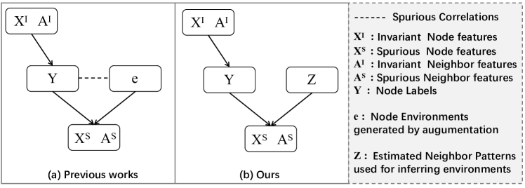
Figure 9: Comparisons between our work and previous graph-based invariant learning works from the causal perspective. Notably, the basic HGNN directly aggregates the selected neighbors’ full features without further separating like the above two types of invariant learning methods.

To help understand our framework well, we first provide the comparison between our work and previous graph-based invarinat learning works as shown in Figure 9. Specifically, the definitions of random variables can be defined as follows: We define $\mathbf{G}$ as a random variable of the input graph, $\mathbf{A}$ as a random variable of node’s neighbor information, $\mathbf{X}$ as a random variable of node’s features, and $\mathbf{Y}$ as a random variable of node’s label vectors. Both node features $\mathbf{X}$ and node neighbor information $\mathbf{A}$ consist of invariant predictive information that determines the label $\mathbf{Y}$ and the spurious information influenced by latent environments $\mathbf{e}$. In this case, we can denote $\mathbf{X}=\left[\mathbf{X}^{I},\mathbf{X}^{S}\right]$ and $\mathbf{A}=\left[\mathbf{A}^{I},\mathbf{A}^{S}\right]$.

Then, we provide a more detailed theoretical analysis of our framework from a casual perspective to identify invariant features.

Casual conditions of $Z$. From the casual perspective, some conditions are also needed for $Z$ to make sure our framework to address the heterophilic graph structure distribution shifts well [24]. Denote the $H(Y|X,A)$ as the expected loss of an optimal classifier over ($X$, $A$, and $Y$), we can clarify the reasonability of utilizing the estimated neighbor patterns as $Z$ auxiliary information to infer environments for invariant prediction based on the following two conditions.

Condition 1 (Invariance Preserving Condition).

Given invariant feature $(X^{I}$ and $A^{I})$ and any function $\rho(\cdot)$, it holds that

$$H(Y|(X^{I},A^{I}),\rho(Z))=H(Y|(X^{I},A^{I})).$$ (14)

Condition 2 (Non-invariance Distinguishing Condition).

For any feature $X^{Sk}\in X^{S}$ or $A^{Sk}\in A^{S}$ ,there exists a function $\rho(\cdot)$ and a constant $C>0$ satisfy:

$$H(Y|(X^{Sk},A^{Sk}))-{H}(Y|(X^{Sk},A^{Sk}),\rho(Z))\geq C.$$ (15)

Condition 1 requires that invariant features $X^{I}$ and $A^{I}$ should keep invariant under any environment split obtained by $\rho(Z)$. Otherwise, if there exists a split where an invariant feature becomes non-invariant, then this feature would introduce a positive penalty as shown in Eq. 13 to further promote the learning of invariant node representation. Exactly, Condition 1 can be met only if $H(Y|(X^{I},A^{I}),Z)=H(Y|(X^{I},A^{I}))$, which means the auxiliary variable $Z$ should be d-separated by invariant feature $X^{I}$ and $A^{I}$. We provide a detailed proof in the appendix A.3. Exactly, the estimated neighbor pattern just describes the similarity between the node and its neighbors as Eq. 11, while the label $Y$ only has the direct causal relationship with $X^{I}$ and $A^{I}$ from the causal perspective. This means the Condition 1 can be met by adopting the estimated neighbor pattern as auxiliary information $Z$ to construct environments.

Condition 2 reveals that for each spurious feature $X^{S}$ and $A^{S}$, there exists at least one environment split where this feature demonstrates non-invariance within the split environment. If a spurious feature doesn’t cause invariance penalties in all environment splits, it can’t be distinguished from true invariant features. As shown in Figure 1(c2), the results of V-Rex are better than ERM, which means even randomly split environments with seeds can have a positive effect on making spurious features produce effective invariance penalty, further promoting the learning of invariant features. It’s more likely to construct comparable or better environments than random seeds under the guidance of the estimated neighbor patterns $Z$. Thus, Condition 2 can also be guaranteed under our defined heterophilic graph structure distribution shit.

Proof of Meeting Condition 1. We show that for all $\rho(\cdot)$, if $H(Y|(X^{I},A^{I}),Z)=H(Y|(X^{I},A^{I}))$ holds, then there will exist that $H(Y|(X^{I},A^{I}),\rho(Z))=H(Y|(X^{I},A^{I}))$.

Proof.

On one hand, because $\rho(Z)$ contains less information than $Z$, we have

$$H(Y|(X^{I},A^{I}),\rho(Z))\geq H(Y|(X^{I},A^{I}),Z)=H(Y|(X^{I},A^{I})).$$

On the other hand, $(X^{I},A^{I})$ and $\rho(Z)$ contain more information than $(X^{I},A^{I})$, so we can get

$$H(Y|(X^{I},A^{I}),\rho(Z))\leq H(Y|(X^{I},A^{I})).$$

Thus, we conclude $H(Y|(X^{I},A^{I}),\rho(Z))=H(Y|(X^{I},A^{I}))$. ∎

Assumptions and Theorem to Identify Invariant Features. In particular, our assumption is consistent with previous invariant learning [24]. So we provide the previous version to support our framework, where $X=[X_{v};X_{s}]$, where the $X_{v}$ refers to the invariant feature and the $X_{s}$ refers to the spurious feature.

Assumption 1.

For a given feature mask $\Phi$ and any constant $\epsilon>0$, there exists $f\in F$ such that $E[l(f(\Phi(X)),Y)]\leq H(Y|\Phi(X))+\epsilon.$

Assumption 2.

If a feature violates the invariance constraint, adding another feature would not make the penalty vanish, i.e., there exists a constant $delta>0$ so that for spurious feature $X_{1}\subset X_{s}$ and any feature $X_{2}\subset X$,

$H(Y|X_{1},X_{2})-{H}(Y|\rho(Z),X_{1},X_{2})\geq\delta\left(H(Y|X_{1})-{H}(Y|\rho(Z),X_{1})\right)$.

Assumption 3.

For any distinct features $X_{1}$, $X_{2}$, $H(Y|X_{1},X_{2})\leq H(Y|X_{1})-\gamma$ with fixed $\gamma>0$.

Exactly, Assumption 1 is a common assumption that requires the function space $F$ be rich enough such that, given $\Phi$, there exists $f\in F$ that can fit $P(Y|\Phi(X))$ well. Assumption 2 aims to ensure a sufficient positive penalty if a spurious feature is included. Assumption 3 indicates that any feature contains some useful information w.r.t. $Y$, which cannot be explained by other features. Otherwise, we can simply remove such a feature, as it does not affect prediction.

The theorem to identify invariant features can be defined:

Theorem 1.

Depending on the Assumptions 1-3 and Conditions 1-2, if $\epsilon<\frac{C\gamma\delta}{4\gamma+2C\delta H(Y)}$ and $\lambda\in[\frac{H(Y)+1/2\delta C}{\delta C-4\epsilon}-\frac{1}{2},\frac{\gamma}{4\epsilon}-\frac{1}{2}]$, then we will have $\hat{L}(\Phi_{v})<\hat{L}(\Phi)$ for all $\Phi\neq\Phi_{v}$, where $H(Y)$ denotes the entropy of $Y$.

A.4 Experimental Setup

Datasets. We adopt six commonly used heterophilic graph datasets as shown in Table 4 [31, 23], to verify the effectiveness of HEI. Notably, considering that we should further split the test datasets to construct different evaluation settings. Those excessive small-scale heterophilic graph datasets, such as Texa, Cornell, and Wisconsin [31], are not fit and chosen for evaluation due to their unstable outcomes. Moreover, in real-world settings, we can’t know whether the input graph is homophilic or heterophilic in advance. Thus, we also provide comparison experiments and discussions for homophilic graphs in the Appendix A.5.

Settings. Based on previous dataset splits, we construct two different settings to evaluate the effectiveness and robustness of methods: (i) Standard Settings: We sort the test nodes based on their nodes’ homophily values and acquire the median. The part that is higher than the median is defined as High Hom Test, while the rest is defined as Low Hom Test. The model is trained on the previous train dataset and evaluated on more fine-grained test groups; (ii) Simulation Settings where exists severe distribution shifts.: We sort and split the train and test nodes simultaneously adopting the same strategy of (i). The model is trained on the Low/High Hom Train and evaluated on the High/Low Hom Test.

Backbones. Previous studies on heterophilic graphs mainly focus on effective backbone designs. To further verify our work is orthogonal to previous HGNN works, we adapt our framework to two existing SOTA and scalable backbones with different foundations, LINKX (MLP-based) [23] and GloGNN++ (GNN-based) [22]. In this way, the improvements can be attributed to the design to cope with the neglected structure distribution shifts on heterophilic graphs.

Baselines. Denote the results of the backbone itself as ERM(Base). We mainly compare HEI with previous graph-based methods that can handle agnostic distribution shifts on node-level tasks, which can be categorized into: (i) without environment augmentation methods (Renode [6], SRGNN [42]); (ii) with environment augmentation methods (EERM [37], BAGNN [12], FLOOD [27]). Notably, though we can utilize estimated neighbor patterns as auxiliary information to infer latent environments as stated above, the true environment label is still unavailable. So we don’t compare with those traditional invariant learning methods that rely on the explicit environment labels there, e.g. IRM [3], V-Rex [20] and GroupDRO [33]. More details can be seen in the Appendix A.6.

Table 4: Statistics for our used heterophilic graph datasets.

Dataset	Chameleon	Squirrel	Actor	Penn94	arXiv-year	twitch-gamer
Nodes	2277	5201	7600	41554	169343	168114
Edges	36101	216933	29926	1362229	1166243	6797557
Feat	2325	2089	931	5	128	7
Class	5	5	5	2	5	2
Edge hom.	0.23	0.22	0.22	0.47	0.222	0.545

A.5 More Experimental Results

We provide more experimental results to further show the effectiveness of the proposed HEI in addressing heterophilic graph structure distribution shifts.

RQ2: Additional Experiments on Simulation Settings using GloGNN++ as backbone. We also conduct experiments under severe distribution shifts using GloGNN++ as the backbone. As shown in Figure LABEL:GloGNN_large, our proposed method can acquire superior or comparable results than previous methods to handle graph structure distribution shifts, which further verifies the effectiveness and robustness of our design.

RQ3: Additional Experiments to explore the effect of similarity-based metric on large-scale datasets We provide the additional experiments about RQ3 there as shown in Table 6.

RQ4: Sensitive analysis. We provide the experimental results about RQ4 there as shown in Figure LABEL:environments_number.

Experiments on Homophilic Graph Datasets. Considering the fact that in real-world settings, we can’t know whether the input graph is homophilic or heterophilic in advance. Thus, we also provide comparison experiments and discussions for homophilic graphs. As shown in Table 7, from the results, we observe that our method can achieve consistent comparable performance to other baselines. But exactly, the improvements by these methods are all minor compared with the base result. That’s because the homophilic graph is not related to our settings. After all, homophilic graph datasets mean the neighbor pattern distribution between the train and test are nearly the same, which is not suitable to clarify our defined distribution shifts. The performance gap between the low home test and the high home test can support our analysis.

RQ5:Efficiency Studies. As shown in Table 5, referring to [22], we provide the time(seconds) to train the model until it converges which keeps the stable accuracy score on the validation set. From the results, we can conclude that the extra time cost can be acceptable compared with the base(backbone itself).

Table 5: Efficiency studies of HEI, where the report scores show the time(seconds) to train the model until converge that keeps the stable accuracy score on the validation set. Referring to [22], we adopt the GloGNN++ as the backbone there.

Methods	Penn94	arxiv-year	twitch-gamer
Base	22.3	7.2	40.5
Renode	23.5	8.5	41.2
SRGNN	24.9	9.1	41.0
EERM	24.7	8.8	41.5
BAGNN	24.8	9.1	42.1
FLOOD	24.5	8.8	41.8
HEI(Ours)	24.5	9.0	41.9

Table 6: Comparison experiments on large-scale datasets when we respectively adopt local similarity(Local Sim), post-aggregation similarity (Agg Sim), and SimRank as indicators to estimate nodes’ neighbor patterns so as to infer latent environments under Standard settings.

Backbones	Methods	Penn94			arxiv-year			twitch-gamer
		Full Test	High Hom Test	Low Hom Test	Full Test	High Hom Test	Low Hom Test	Full Test	High Hom Test	Low Hom Test
LINKX	HEI (Local Sim)	85.12 ± 0.21	88.28 ± 0.33	82.15 ± 0.59	54.41 ± 0.21	64.23 ± 0.47	48.29 ± 0.22	66.18 ± 0.12	83.75 ± 0.34	48.12 ± 0.47
	HEI (Agg Sim)	85.21 ± 0.17	88.29 ± 0.38	82.22 ± 0.54	54.45 ± 0.23	64.33 ± 0.49	48.33 ± 0.32	66.21 ± 0.15	83..85 ± 0.39	48.45 ± 0.57
	HEI (SimRank)	85.52 ± 0.31	88.44 ± 0.38	82.62 ± 0.54	54.65 ± 0.23	64.53 ± 0.63	48.63 ± 0.32	66.29 ± 0.15	84.03 ± 0.38	49.02 ± 0.57
GloGNN++	HEI (Local Sim)	86.08 ± 0.24	89.70 ± 0.64	82.18 ± 0.37	54.42 ± 0.24	64.48 ± 1.54	48.55 ± 0.64	66.30 ± 0.18	83.21 ± 0.68	49.00 ± 0.67
	HEI (Agg Sim)	86.15 ± 0.25	89.70 ± 0.69	82.43 ± 0.38	54.44 ± 0.25	64.51 ± 1.54	48.69 ± 0.81	66.34 ± 0.21	83.19 ± 0.78	49.14 ± 0.57
	HEI (SimRank)	86.48 ± 0.28	89.72 ± 0.65	83.09 ± 0.39	54.49 ± 0.20	64.59 ± 1.24	48.99 ± 0.75	66.39 ± 0.17	83.23 ± 0.68	49.50 ± 0.57

Table 7: Performance comparison on homophilic graph datasets under Standard Settings. The reported scores denote the classification accuracy (%) and error bar (±) over 10 trials. We highlight the best score on each dataset in bold and the second score with underline.

Backbones	Methods	CiteSeer			PubMed			Cora
		Full Test	High Hom Test	Low Hom Test	Full Test	High Hom Test	Low Hom Test	Full Test	High Hom Test	Low Hom Test
LINKX	ERM(Base)	73.19 ± 0.99	73.89 ± 1.51	72.79 ± 1.47	87.86 ± 0.77	88.49 ± 1.37	87.19 ± 1.51	84.64 ± 1.13	85.13 ± 1.83	83.85 ± 1.99
	ReNode	73.25 ± 0.89	74.00 ± 1.21	72.89 ± 1.87	87.91 ± 0.72	88.58 ± 1.42	87.21 ± 1.71	84.70 ± 1.23	85.28 ± 1.99	84.24 ± 2.13
	SRGNN	73.27 ± 0.99	74.03 ± 1.11	72.85 ± 1.87	87.96 ± 0.81	88.68 ± 1.72	87.31 ± 1.51	84.71 ± 1.25	85.22 ± 1.87	84.34 ± 2.03
	EERM	73.17 ± 0.79	73.81 ± 1.45	73.09 ± 1.65	87.96 ± 0.84	88.59 ± 1.32	87.29 ± 1.63	84.62 ± 1.37	85.14 ± 1.63	83.87 ± 2.03
	BAGNN	73.33 ± 0.88	73.99 ± 1.61	73.19 ± 1.63	88.01 ± 0.94	88.78 ± 1.57	87.69 ± 1.39	84.60 ± 1.28	85.24 ± 1.83	83.84 ± 2.41
	FLOOD	73.34 ± 0.91	73.95 ± 1.55	73.22 ± 1.67	88.05 ± 0.95	88.84 ± 1.62	87.81 ± 1.59	84.72 ± 1.41	85.35 ± 1.63	83.99 ± 2.51
	HEI(Ours)	73.51 ± 0.81	74.18 ± 1.25	73.42 ± 1.85	88.50 ± 0.97	89.01 ± 1.24	87.84 ± 1.92	85.17 ± 1.53	85.44 ± 1.83	84.84 ± 1.97
GloGNN++	ERM(Base)	77.22 ± 1.78	78.15 ± 2.55	76.79 ± 2.54	89.24 ± 0.39	90.62 ± 0.99	88.75 ± 1.28	88.33± 1.09	90.06 ± 1.52	87.37 ± 1.64
	ReNode	77.31 ± 1.69	78.27 ± 2.48	76.90 ± 2.39	89.25 ± 0.35	90.64 ± 0.87	88.79 ± 1.24	88.39± 1.21	90.11 ± 1.49	87.45 ± 1.57
	SRGNN	77.33 ± 1.65	78.24 ± 2.75	76.91 ± 2.77	89.33 ± 0.51	90.81 ± 1.21	88.99 ± 1.57	88.53± 1.09	90.46 ± 1.53	87.58 ± 1.54
	EERM	77.35 ± 1.81	78.27 ± 2.45	76.89 ± 2.81	89.34 ± 0.39	90.82 ± 1.09	88.95 ± 1.38	88.39± 1.21	90.36 ± 1.42	87.47 ± 1.74
	BAGNN	77.42 ± 1.81	78.35 ± 2.81	76.89 ± 2.42	89.37 ± 0.45	90.87 ± 1.29	88.99 ± 1.58	88.49± 1.31	90.39 ± 1.47	87.81 ± 1.64
	FLOOD	77.43 ± 1.79	78.39 ± 2.51	76.95 ± 2.37	89.41 ± 0.51	90.91 ± 1.29	89.08 ± 1.58	88.51 ± 1.27	90.40 ± 1.51	87.88 ± 1.69
	HEI(Ours)	77.45 ± 1.81	78.45 ± 2.59	77.00 ± 2.87	89.49± 0.39	91.12 ± 0.99	89.18 ± 1.33	88.73± 1.19	90.86 ± 1.39	88.17 ± 1.74

A.6 Implementation Details

We provide detailed implementation details for our experiments. The code to reproduce our experiments can be seen in supplementary material(in a ZIP format).

ERM(Base), It corresponds to the results of the backbone itself. We just entirely follow previous works [23, 22] under our constructed settings.

SRGNN[42], Shift-Robust GNN is a framework inspired by domain adaption, which means it needs prior knowledge from the target domain. Specifically, it strives to adapt a biased sample of labeled nodes to more closely conform to the distributional characteristics present in an IID sample of the graph. In our experiments, we utilize the estimated neighbor distribution information to evaluate the distribution of the source domain and target domain. Apart from this, we entirely follow this work to address graph structure distribution shifts on heterophilic graphs.

Renode[6], in our experiments, it is an extension of the original Renode, which is a model-agnostic training weight schedule mechanism to cope with topology-imbalance problems for semi-supervised node classification. Specifically, they devise a cosine annealing mechanism for the training node weights based on their Totoro values. The Totoro values involve topology information and can also integrate with quantity-imbalanced methods as the paper shown. Therefore, this method can also be seen as a baseline which can copy with agnostic distribution shifts. We adopt the same reweight strategy as the paper stated, and the Totoro values can also describe the neighbor pattern to a certain extent.

EERM[37], Explore-to-Extrapolate Risk Minimization (EERM) is an invariant learning approach that facilitates graph neural networks to leverage invariance principles for prediction. As stated in the paper, EERM resorts to multiple context explorers that are adversarially trained to construct diverse environments with augmentation. Then, following the principle of variance of risks, it utilizes the variance from multiple virtual environments as regularization to help model training. We entirely follow this work to address graph structure distribution shifts on heterophilic graphs.

BAGNN[12], Bias-aware(BA) GNN is also a method that deals with agnostic distribution shifts on graphs from the perspective of invariant learning. Specifically, it can be summarized into two steps: the environment clustering module assigns nodes to environments with minimization loss, and the invariant graph learning module learns invariant representation across environments with minimization loss. During the process of environment clustering, it adopts the masking strategy with graph augmentation. We entirely follow this work to address graph structure distribution shifts on heterophilic graphs.

FLOOD[27], it is also a a flexible invariant learning framework for OOD generalization on graphs. Specifically, it includes two key modules, invariant learning, and bootstrapped learning. The invariant learning modules construct multiple environments from graph data augmentation and learn invariant representation under risk extrapolation. Besides, the bootstrapped learning component is inspired by test time adaptation, which proposes to train a shared graph encoder with the invariant learning part according to the test distribution. We entirely follow this work to address graph structure distribution shifts on heterophilic graphs.

HEI (Ours), our training process can be concluded as follows: Given a heterophilic graph input, we first calculate the SimRank for each node in advance. Then, based on Equation 13, we collectively learn environment partition and invariant representation on heterophilic graphs, assisted by SimRank, to address graph structure distribution shifts on heterophilic graphs. Therefore, we save the processed SimRank values on nodes on the graph in advance and transfer them into tensors for the training. For training details, we should warm up for some epochs to avoid the learned environments in the initial stage that are not effective, which may influence the optimization of models. So at the beginning warm-up stage, we adopt the ERM strategy that is equal to the Base stage. After that, we adopt our proposed framework to learn an invariance penalty to improve model performance. For the range of parameters, we first execute experiments using basic backbones to get the best parameters of num-layers and hidden channels on different datasets. Then, we fix the num-layers and hidden channels to adjust other parameters, penalty weight$\lambda$) from $\left\{1e-,1e-2,1e-1,1,10,100\right\}$, learning rate from $\left\{1e-2,5e-3,1e-3,5e-4,1e-4\right\}$ and weight decay from $\left\{1e-2,5e-3,1e-3\right\}$. We also provide parameter sensitivity of environment number $k$ in the paper. Moreover, the $\rho$ is a two-layer MLP with the hidden channel from $\left\{16,32,64\right\}$, and its learning rate should be lower than the backbone in our experiments, within the range from $\left\{5e-3,1e-3,5e-4,1e-4\right\}$.

References

- (1) Sami Abu-El-Haija, Bryan Perozzi, Amol Kapoor, Nazanin Alipourfard, Kristina Lerman, Hrayr Harutyunyan, Greg Ver Steeg, and Aram Galstyan. Mixhop: Higher-order graph convolutional architectures via sparsified neighborhood mixing. In international conference on machine learning, pages 21–29. PMLR, 2019.
- (2) Kartik Ahuja, Jun Wang, Amit Dhurandhar, Karthikeyan Shanmugam, and Kush R Varshney. Empirical or invariant risk minimization? a sample complexity perspective. arXiv preprint arXiv:2010.16412, 2020.
- (3) Martin Arjovsky, Léon Bottou, Ishaan Gulrajani, and David Lopez-Paz. Invariant risk minimization. arXiv preprint arXiv:1907.02893, 2019.
- (4) Shiyu Chang, Yang Zhang, Mo Yu, and Tommi Jaakkola. Invariant rationalization. In International Conference on Machine Learning, pages 1448–1458. PMLR, 2020.
- (5) Deli Chen, Yankai Lin, Wei Li, Peng Li, Jie Zhou, and Xu Sun. Measuring and relieving the over-smoothing problem for graph neural networks from the topological view. In Proceedings of the AAAI conference on artificial intelligence, volume 34, pages 3438–3445, 2020.
- (6) Deli Chen, Yankai Lin, Guangxiang Zhao, Xuancheng Ren, Peng Li, Jie Zhou, and Xu Sun. Topology-imbalance learning for semi-supervised node classification. Advances in Neural Information Processing Systems, 34:29885–29897, 2021.
- (7) Ming Chen, Zhewei Wei, Zengfeng Huang, Bolin Ding, and Yaliang Li. Simple and deep graph convolutional networks. In International conference on machine learning, pages 1725–1735. PMLR, 2020.
- (8) Yongqiang Chen, Yatao Bian, Kaiwen Zhou, Binghui Xie, Bo Han, and James Cheng. Does invariant graph learning via environment augmentation learn invariance? arXiv preprint arXiv:2310.19035, 2023.
- (9) Yongqiang Chen, Yonggang Zhang, Yatao Bian, Han Yang, MA Kaili, Binghui Xie, Tongliang Liu, Bo Han, and James Cheng. Learning causally invariant representations for out-of-distribution generalization on graphs. Advances in Neural Information Processing Systems, 35:22131–22148, 2022.
- (10) Yuhan Chen, Yihong Luo, Jing Tang, Liang Yang, Siya Qiu, Chuan Wang, and Xiaochun Cao. Lsgnn: Towards general graph neural network in node classification by local similarity. arXiv preprint arXiv:2305.04225, 2023.
- (11) Zhengyu Chen, Jixie Ge, Heshen Zhan, Siteng Huang, and Donglin Wang. Pareto self-supervised training for few-shot learning. In Proceedings of the IEEE/CVF Conference on Computer Vision and Pattern Recognition, pages 13663–13672, 2021.
- (12) Zhengyu Chen, Teng Xiao, and Kun Kuang. Ba-gnn: On learning bias-aware graph neural network. In 2022 IEEE 38th International Conference on Data Engineering (ICDE), pages 3012–3024. IEEE, 2022.
- (13) Zhengyu Chen, Teng Xiao, Kun Kuang, Zheqi Lv, Min Zhang, Jinluan Yang, Chengqiang Lu, Hongxia Yang, and Fei Wu. Learning to reweight for generalizable graph neural network. In Proceedings of the AAAI Conference on Artificial Intelligence, volume 38, pages 8320–8328, 2024.
- (14) Zhengyu Chen, Teng Xiao, Donglin Wang, and Min Zhang. Pareto graph self-supervised learning. In ICASSP 2024-2024 IEEE International Conference on Acoustics, Speech and Signal Processing (ICASSP), pages 6630–6634. IEEE, 2024.
- (15) Eli Chien, Jianhao Peng, Pan Li, and Olgica Milenkovic. Adaptive universal generalized pagerank graph neural network. arXiv preprint arXiv:2006.07988, 2020.
- (16) Shurui Gui, Xiner Li, Limei Wang, and Shuiwang Ji. Good: A graph out-of-distribution benchmark. Advances in Neural Information Processing Systems, 35:2059–2073, 2022.
- (17) Dongxiao He, Chundong Liang, Huixin Liu, Mingxiang Wen, Pengfei Jiao, and Zhiyong Feng. Block modeling-guided graph convolutional neural networks. In Proceedings of the AAAI conference on artificial intelligence, volume 36, pages 4022–4029, 2022.
- (18) Di Jin, Zhizhi Yu, Cuiying Huo, Rui Wang, Xiao Wang, Dongxiao He, and Jiawei Han. Universal graph convolutional networks. Advances in Neural Information Processing Systems, 34:10654–10664, 2021.
- (19) Wei Jin, Tyler Derr, Yiqi Wang, Yao Ma, Zitao Liu, and Jiliang Tang. Node similarity preserving graph convolutional networks. In Proceedings of the 14th ACM international conference on web search and data mining, pages 148–156, 2021.
- (20) David Krueger, Ethan Caballero, Joern-Henrik Jacobsen, Amy Zhang, Jonathan Binas, Dinghuai Zhang, Remi Le Priol, and Aaron Courville. Out-of-distribution generalization via risk extrapolation (rex). In International Conference on Machine Learning, pages 5815–5826. PMLR, 2021.
- (21) Haoyang Li, Ziwei Zhang, Xin Wang, and Wenwu Zhu. Learning invariant graph representations for out-of-distribution generalization. Advances in Neural Information Processing Systems, 35:11828–11841, 2022.
- (22) Xiang Li, Renyu Zhu, Yao Cheng, Caihua Shan, Siqiang Luo, Dongsheng Li, and Weining Qian. Finding global homophily in graph neural networks when meeting heterophily. In International Conference on Machine Learning, pages 13242–13256. PMLR, 2022.
- (23) Derek Lim, Felix Hohne, Xiuyu Li, Sijia Linda Huang, Vaishnavi Gupta, Omkar Bhalerao, and Ser Nam Lim. Large scale learning on non-homophilous graphs: New benchmarks and strong simple methods. Advances in Neural Information Processing Systems, 34:20887–20902, 2021.
- (24) Yong Lin, Shengyu Zhu, Lu Tan, and Peng Cui. Zin: When and how to learn invariance without environment partition? Advances in Neural Information Processing Systems, 35:24529–24542, 2022.
- (25) Gang Liu, Tong Zhao, Jiaxin Xu, Tengfei Luo, and Meng Jiang. Graph rationalization with environment-based augmentations. In Proceedings of the 28th ACM SIGKDD Conference on Knowledge Discovery and Data Mining, pages 1069–1078, 2022.
- (26) Haoyu Liu, Ningyi Liao, and Siqiang Luo. Simga: A simple and effective heterophilous graph neural network with efficient global aggregation. arXiv preprint arXiv:2305.09958, 2023.
- (27) Yang Liu, Xiang Ao, Fuli Feng, Yunshan Ma, Kuan Li, Tat-Seng Chua, and Qing He. Flood: A flexible invariant learning framework for out-of-distribution generalization on graphs. In Proceedings of the 29th ACM SIGKDD Conference on Knowledge Discovery and Data Mining, pages 1548–1558, 2023.
- (28) Sitao Luan, Chenqing Hua, Qincheng Lu, Jiaqi Zhu, Mingde Zhao, Shuyuan Zhang, Xiao-Wen Chang, and Doina Precup. Is heterophily a real nightmare for graph neural networks to do node classification? arXiv preprint arXiv:2109.05641, 2021.
- (29) Sitao Luan, Chenqing Hua, Qincheng Lu, Jiaqi Zhu, Mingde Zhao, Shuyuan Zhang, Xiao-Wen Chang, and Doina Precup. Revisiting heterophily for graph neural networks. Advances in neural information processing systems, 35:1362–1375, 2022.
- (30) Haitao Mao, Zhikai Chen, Wei Jin, Haoyu Han, Yao Ma, Tong Zhao, Neil Shah, and Jiliang Tang. Demystifying structural disparity in graph neural networks: Can one size fit all? arXiv preprint arXiv:2306.01323, 2023.
- (31) Hongbin Pei, Bingzhe Wei, Kevin Chen-Chuan Chang, Yu Lei, and Bo Yang. Geom-gcn: Geometric graph convolutional networks. arXiv preprint arXiv:2002.05287, 2020.
- (32) Yu Rong, Wenbing Huang, Tingyang Xu, and Junzhou Huang. Dropedge: Towards deep graph convolutional networks on node classification. arXiv preprint arXiv:1907.10903, 2019.
- (33) Shiori Sagawa, Pang Wei Koh, Tatsunori B Hashimoto, and Percy Liang. Distributionally robust neural networks for group shifts: On the importance of regularization for worst-case generalization. arXiv preprint arXiv:1911.08731, 2019.
- (34) Susheel Suresh, Vinith Budde, Jennifer Neville, Pan Li, and Jianzhu Ma. Breaking the limit of graph neural networks by improving the assortativity of graphs with local mixing patterns. In Proceedings of the 27th ACM SIGKDD Conference on Knowledge Discovery & Data Mining, pages 1541–1551, 2021.
- (35) Tao Wang, Di Jin, Rui Wang, Dongxiao He, and Yuxiao Huang. Powerful graph convolutional networks with adaptive propagation mechanism for homophily and heterophily. In Proceedings of the AAAI conference on artificial intelligence, volume 36, pages 4210–4218, 2022.
- (36) Yu Wang and Tyler Derr. Tree decomposed graph neural network. In Proceedings of the 30th ACM international conference on information & knowledge management, pages 2040–2049, 2021.
- (37) Qitian Wu, Hengrui Zhang, Junchi Yan, and David Wipf. Handling distribution shifts on graphs: An invariance perspective. arXiv preprint arXiv:2202.02466, 2022.
- (38) Ying-Xin Wu, Xiang Wang, An Zhang, Xiangnan He, and Tat-Seng Chua. Discovering invariant rationales for graph neural networks. arXiv preprint arXiv:2201.12872, 2022.
- (39) Ruihao Zhang, Zhengyu Chen, Teng Xiao, Yueyang Wang, and Kun Kuang. Discovering invariant neighborhood patterns for heterophilic graphs. arXiv preprint arXiv:2403.10572, 2024.
- (40) Xin Zheng, Yixin Liu, Shirui Pan, Miao Zhang, Di Jin, and Philip S Yu. Graph neural networks for graphs with heterophily: A survey. arXiv preprint arXiv:2202.07082, 2022.
- (41) Jiong Zhu, Yujun Yan, Lingxiao Zhao, Mark Heimann, Leman Akoglu, and Danai Koutra. Beyond homophily in graph neural networks: Current limitations and effective designs. Advances in neural information processing systems, 33:7793–7804, 2020.
- (42) Qi Zhu, Natalia Ponomareva, Jiawei Han, and Bryan Perozzi. Shift-robust gnns: Overcoming the limitations of localized graph training data. Advances in Neural Information Processing Systems, 34:27965–27977, 2021.