Undominated monopoly regulation

Abstract

We study undominated mechanisms with transfers for regulating a monopolist who privately observes the marginal cost of production. We show that in any undominated mechanism, there is a quantity floor, which depends only on the primitives, and the regulator’s operation decision is stochastic only if the monopolist produces at the quantity floor. We provide a near-complete characterization of the set of undominated mechanisms and use it to (a) provide a foundation for deterministic mechanisms, (b) show that the efficient mechanism is dominated, and (c) derive a max-min optimal regulatory mechanism.

Keywords: regulation, undominated mechanisms, floor randomized mechanisms, downward distortion.

JEL Classification: D82, L51

1 Introduction

We consider the problem of regulating a monopolist who privately observes the marginal cost of production. The regulator’s payoff is a weighted sum of the consumer surplus and the monopolist’s profit, with a strictly smaller weight on the monopolist’s profit. Given such preferences, the regulator would like to maximize the consumer surplus irrespective of the cost (type) of the monopolist. However, incentive constraints imply that increasing consumer surplus at a given type reduces the consumer surplus at lower types. A seminal paper, Baron and Myerson (1982), studies the optimal resolution of this trade-off when the regulator uses transfers and maximizes the expected payoff with respect to a prior over the space of plausible marginal costs. Most of the subsequent literature, both with and without transfers, assumed expected payoff maximization by the regulator subject to incentive (IC) and participation (IR) constraints of the monopolist (see Armstrong and Sappington (2006) for an extensive survey).

This paper takes the first step in understanding the prior-free criterion of undomination in the context of regulatory mechanisms. A regulatory mechanism must specify an operation decision, which may be stochastic; a quantity decision, which is contingent on the monopolist operating; and a transfer decision on the amount of subsidy/tax to the monopolist, which is also contingent on the monopolist operating. A regulatory mechanism is undominated if no other mechanism gives the regulator a strictly higher payoff at some marginal cost of the monopolist without lowering the regulator’s payoff at other costs. Such prior-free undominated mechanisms are relevant particularly when the regulator lacks confidence in the belief over the plausible marginal costs or fears ex-post criticism of the subjective belief used while choosing the regulatory mechanism. The concept of undomination is also useful for refining the set of worst-case optimal mechanisms when it is not a singleton.

Our first main result shows that an undominated regulatory mechanism must be a floor randomized mechanism. A floor randomized mechanism is defined by partitioning the type space into three disjoint intervals (with the possibility that some of these intervals may be empty) and a quantity floor $\hat{q}$, which we define precisely later. In the first interval (containing the low-cost types), the (monopolist) firm operates for sure and produces quantity higher than the quantity floor $\hat{q}$. In the second interval, with intermediate-cost types, the firm operates with positive probability (possibly less than one) and produces quantity $\hat{q}$. The firm is shut in the third interval, which contains high-cost types. Thus, the operation decision is stochastic only at the quantity floor $\hat{q}$.

A general incentive compatible (IC) and individually rational (IR) mechanism is characterized by the monotonicity of the product of quantity and operation probability, and an envelope formula specifying the transfer. On the other hand, floor randomized mechanisms (which are IC and IR) have several structural properties that make them easier to handle: (i) whenever the monopolist is allowed to operate, the quantity produced is bounded below by $\hat{q}$; (ii) operation decision is stochastic only when the quantity produced equals $\hat{q}$; (iii) both quantity and operation decisions are monotone.

Using these properties of floor randomized mechanisms, we derive two further necessary conditions for undomination. The first condition is what we call downward distortion. It requires that the quantity produced at every type be lower than the efficient quantity at that type. Thus, there is a type-dependent upper bound on the quantity to be produced (the quantity floor $\hat{q}$ is type-independent). The second condition is technical and requires the product of the quantity and the operation decisions to be left continuous. Thus, we show that every undominated mechanism is a floor randomized mechanism satisfying downward distortion and left-continuity. Conversely, every floor randomized mechanism satisfying left-continuity and a stricter version of downward distortion is undominated. Thus, undomination, despite being a weak criterion, puts significant structure on the set of IC and IR mechanisms.

Our analysis has three critical implications for regulation design. First, we show that for every IC and IR mechanism $M$ and for every prior over the marginal costs, there exists a deterministic IC and IR mechanism that generates more expected payoff for the regulator than $M$. This provides a foundation for deterministic mechanisms in our model and explains why the optimal regulatory mechanism in Baron and Myerson (1982) is deterministic. The second implication concerns the efficient mechanism, where the firm always operates and produces efficient quantity (maximizing total surplus). We show that the efficient mechanism is dominated. The third implication is for an ambiguity-averse regulator who evaluates any mechanism by the worst expected payoff it generates over a set of priors. We call the mechanism that gives the highest such worst payoff as max-min optimal mechanism. We establish that if the set of priors contains a prior that (first-order) stochastically dominates every other prior in the set, then the max-min optimal mechanism is the optimal mechanism for that prior.

As an essential step in proving the result on max-min optimal regulatory mechanisms, we show that undominated mechanisms are monotonic. The regulator’s expected payoff increases as the distribution over marginal cost decreases in the first-order sense. In general, an arbitrary IC regulatory mechanism need not be monotonic. This observation contrasts sharply with IC mechanisms for selling a single good. As Hart and Reny (2015) shows, every IC mechanism for selling a single good is monotonic.

The rest of the paper is organized as follows. Section 2 describes the model. In Section 3, we discuss floor randomized mechanisms and show it is without loss to restrict our search of undominated mechanisms in the class of floor randomized mechanisms. Section 4 gives a near-complete characterization of undominated mechanisms. We discuss the implications of our results for regulation design in Section 5. Finally, related literature is discussed in Section 6, and Appendices A-C contain all the proofs.

2 Model

A regulator oversees a market with a unit mass of consumers and a monopolist selling a single product. We begin by describing the market and then discuss the regulatory mechanisms.

2.1 Market

The total cost incurred by the monopolist in producing a quantity $q>0$ of the product is given by $(c+\theta q)$. The parameter $c>0$ denotes the fixed cost which is incurred only when $q>0$. The parameter $\theta>0$ denotes the marginal cost of production for the monopolist. The monopolist is perfectly informed about its fixed cost and marginal cost.

Let $P:\Re_{+}\rightarrow\Re_{+}$ be a strictly decreasing inverse demand function that represents the preferences of the unit mass of consumers. If the monopolist charges a uniform price of $P(q)$, where $q>0$, exactly $q$ units of the product are sold in the market, and the consumers get a total value of

$$V(q) =\int\limits_{0}^{q}P(z)dz.$$

The associated consumer surplus (CS) is given by $\big{(}V(q)-qP(q)\big{)}$ and the profit of the monopolist is $\big{(}qP(q)-\theta q-c\big{)}$. Finally, the total surplus (TS) is the sum of consumer surplus and profit of the monopolist, i.e.,

$$\textsc{TS}(\theta,q)=V(q)-\theta q-c.$$

If zero units are sold, i.e. $q=0$, the consumer surplus, monopolist’s profit, and total surplus are all zero.

Throughout the paper, we impose the following assumptions on the primitives. We assume that the marginal cost $\theta$ can take values in the interval $\Theta\equiv[\underline{\theta},\overline{\theta}]$, where $0<\underline{\theta}<\overline{\theta}$. Further, $P$ satisfies the following conditions.

1. $P$ is continuous and $P(\overline{q})=0$ for some $\overline{q}>0$.

2. $c$ and $\overline{\theta}$ are such that $\textsc{TS}\big{(}\overline{\theta},P^{-1}(\overline{\theta})\big{)}>0$.

Assumptions [A1] is a technical assumption on $P$. Assumption [A2] is a joint condition on $c$, $\overline{\theta}$ and $P^{-1}$. Intuitively, it says that it is “efficient” to let the type with the highest marginal cost operate in the complete information benchmark.

2.2 Regulatory mechanisms

The regulator perfectly knows the fixed cost of the monopolist and the inverse demand function. However, when it comes to the marginal cost, the regulator only knows that it belongs to $\Theta$.

The regulatory apparatus employed in disciplining the behavior of the monopolist can be summarized through a regulatory mechanism $M$. By revelation principle, we focus on direct regulatory mechanisms in which the monopolist first reports the marginal cost $\theta$ to the regulator, who then enforces two decisions $r(\theta)$ and $q(\theta)$ on the monopolist and transfers a contingent subsidy $s(\theta)$ to the monopolist. More specifically, a regulatory mechanism is given by $M\equiv(r,q,s)$, where

• Operation decision. The map $r:\Theta\rightarrow[0,1]$ denotes the probability with which the monopolist is allowed to operate.

• Quantity rule. If the monopolist is allowed to operate, the map $q:\Theta\rightarrow[0,\bar{q}]$ prescribes the quantity to be produced by the monopolist.

• Subsidy rule. If the monopolist is allowed to operate, the map $s:\Theta\rightarrow\Re$ represents the subsidy each type of monopolist receives.

Throughout the paper, we focus attention on regulatory mechanisms such that $q(\theta)=0$ if and only if $r(\theta)=0$. This restriction is without loss and will simplify of the exposition. Given such a regulatory mechanism, $M\equiv(r,q,s)$, the utility of a type $\theta$ monopolist from truthfully reporting its type is

$$u(\theta):=\Big{[}q(\theta)P(q(\theta))-\theta q(\theta)-c+s(\theta)\Big{]}r(\theta).$$ (1)

On the other hand, the corresponding consumer surplus (CS) is

$$\textsc{CS}(\theta,M) =\Big{(}V(q(\theta))-q(\theta)P(q(\theta))-s(\theta)\Big{)}r(\theta)$$

$$=\Big{(}V(q(\theta))-c-\theta q(\theta)\Big{)}r(\theta)-u(\theta)$$ (2)

where (2.2) is obtained by substituting $s(\theta)$ from equation (1). Observe, equation (1) uniquely defines the subsidy $s$ for given $(r,q,u)$. Thus, it is without loss of generality to write a mechanism as $M\equiv(r,q,u)$. On the other hand, we denote a deterministic mechanism, i.e., a mechanism where $r(\theta)\in\{0,1\}$ for all $\theta$, as $M\equiv(q,u)$ by suppressing $r$. We follow this convention throughout the paper.

A regulatory mechanism $(r,q,u)$ is incentive compatible (IC) if for all $\theta,\theta^{\prime}\in\Theta$

$$u(\theta)\geq\Big{[}q(\theta^{\prime})P(q(\theta^{\prime}))-\theta q(\theta^{\prime})-c+s(\theta^{\prime})\Big{]}r(\theta^{\prime})=u(\theta^{\prime})+(\theta^{\prime}-\theta)q(\theta^{\prime})r(\theta^{\prime}).$$

Furthermore, the regulatory mechanism $M$ is individually rational (IR) if $u(\theta)\geq 0$ for all $\theta\in\Theta$. We now state a lemma establishing the exact connection between incentive compatibility and individual rationality of the mechanism $M\equiv(r,q,u)$ and certain properties of $u$. To do so, fix $\theta$ and let $x\in\Re$ be such that

$$u(\theta^{\prime}) \geq u(\theta)+(\theta^{\prime}-\theta)x~{}\qquad~{}\forall~{}\theta^{\prime}\in\Theta.$$

Then, $x$ is called a subgradient of $u$ at $\theta$. Let $\partial u(\theta)$ be the set of all subgradients of $u$ at $\theta$. The following lemma states if $(r,q,u)$ is IC, then $-q(\theta)r(\theta)\in\partial u(\theta)$.

Lemma 1 (Baron and Myerson (1982))

The following are equivalent:

1. $(r,q,u)$ is IC.

2. $u$ is convex, decreasing, and for all $\theta\in\Theta$

   $$-q(\theta)r(\theta) \in\partial u(\theta).$$

3. $q(\theta)r(\theta)$ is decreasing and for all $\theta\in\Theta$

   $$u(\theta) =u(\bar{\theta})+\int\limits_{\theta}^{\bar{\theta}}q(z)r(z)dz.$$

Further, $(r,q,u)$ is IR if and only if $u(\overline{\theta})\geq 0$.

In standard screening problems, a single monotone function characterizes incentive compatibility (for instance, in single-object auctions, it is the increasing allocation rule). By contrast, in our setup, the incentive compatibility is characterized by the product $q(\theta)r(\theta)$ of two potentially non-monotonic functions $q$ and $r$. By Lemma 1, this product must decrease in $\theta$ for a mechanism $(q,r,u)$ to be IC.

2.3 Regulator’s surplus and undominated mechanisms

If the monopolist is of type $\theta$, the regulator’s surplus from an IC and IR mechanism $M\equiv(r,q,u)$ is

$$\textsc{RS}_{\alpha}(\theta,M) =\textsc{CS}(\theta,M)+\alpha u(\theta),$$

where $\alpha\in[0,1)$ is the weight the regulator puts on the monopolist’s profit. We can further simplify the regulator’s surplus using equation (2.2) to

$$\textsc{RS}_{\alpha}(\theta,M) =r(\theta)\Big{(}V(q(\theta))-c-\theta q(\theta)\Big{)}-(1-\alpha)u(\theta)$$ (3)

$$=r(\theta)\textsc{TS}(\theta,q(\theta))-(1-\alpha)u(\theta)$$ (4)

Thus, the regulator’s surplus can be separated into two parts: the total surplus, which is independent of $\alpha$, and the weighted disutility from the rent paid to the monopolist. The regulator is concerned about total surplus as well as how the total surplus is distributed across the consumers and the monopolist. As $\alpha$ decreases, the distributional concerns of the regulator get stronger. The extreme scenario is when $\alpha=0$, where the regulator’s surplus equals consumer surplus.

We now introduce a prior-free notion of comparing two IC and IR mechanisms.

Definition 1

An IC and IR mechanism $\widetilde{M}$ dominates an IC and IR mechanism $M$ if

$$\textsc{RS}_{\alpha}(\theta,\widetilde{M})\geq\textsc{RS}_{\alpha}(\theta,M)~{}\qquad~{}\forall~{}\theta\in\Theta$$

with strict inequality holding for some $\theta$. In this case, we say $M$ is dominated.

An IC and IR mechanism $M$ is undominated if it is not dominated.

In what follows, we aim to characterize the set of undominated mechanisms.

2.4 Remarks on the model

Some remarks are in order about the modelling of regulatory mechanisms. First, it appears that the regulatory mechanism only controls quantity, and price is determined from inverse demand function. However, we can recast the mechanism to control price, and quantity can be determined by the demand function (as is done in Armstrong and Sappington (2004)).

Second, our regulatory mechanisms use transfers. These transfers come from the consumers and go to the firm (if they are negative, these are taxes collected from the firm that go to the consumers). Implicitly, we assume a budget-balance constraint for the regulator. This is standard in the literature that follows Baron and Myerson (1982) - for departures, see Laffont and Tirole (1986).

Just like us, Baron and Myerson (1982) assume that the type of the monopolist is a single dimensional parameter $\theta$ that affects the cost in a linear way. However, in their model $\theta$ affects both the fixed cost and the marginal cost: the total cost of producing quantity $q$ in their model is $k_{0}+k_{1}\theta+(c_{0}+c_{1}\theta)q$ for a monopolist with type $\theta$. Thus, setting $k_{0}=c,k_{1}=0,c_{0}=0,c_{1}=1$, we get our model. Similar to Amador and Bagwell (2022), this simplification allows us to convey the intuition for our results transparently.

3 Floor randomized mechanisms

This section introduces a subclass of IC and IR mechanisms called floor randomized mechanisms. Every IC and IR mechanism can be transformed into a unique floor randomized mechanism. Our main result will show that converting an arbitrary mechanism to a floor randomized mechanism improves the regulator’s surplus at every type.

As an essential step in defining a floor randomized mechanism, we first describe the quantity floor, $\hat{q}$, which is the unique solution to the following equation:

$$V(q)-qP(q) =c.$$

The LHS is the consumer surplus when the monopolist produces quantity $q$ in absence of any regulation. The equation solves for quantity $\hat{q}$ where this consumer surplus equals fixed cost. To see that a unique positive solution exists, note that $V(q)-qP(q)$ is a strictly increasing function with $\lim_{q\rightarrow 0}V(q)-qP(q)$ equals zero and $V(\overline{q})-\overline{q}P(\overline{q})>c$, where the latter inequality follows from Assumption [A2].

Next, we define a floor randomized mechanism where we use the notation $I\succ I^{\prime}$ for any pair of disjoint intervals $I,I^{\prime}\subseteq\Theta$ to mean $x>y$ for every $x\in I$ and every $y\in I^{\prime}$.

Definition 2

An IC and IR mechanism $(r,q,u)$ is floor randomized if $u(\bar{\theta})=0$ and the type space $\Theta$ can be partitioned into three disjoint intervals $\Theta_{1},\Theta_{01},\Theta_{0}$ such that $\Theta_{0}\succ\Theta_{01}\succ\Theta_{1}$ and

$$q(\theta) \geq\hat{q}~{}~{}{\rm and}~{}~{}r(\theta)=1~{}\qquad~{}\forall~{}\theta\in\Theta_{1}$$

$$q(\theta) =\hat{q}~{}~{}{\rm and}~{}~{}r(\theta)\in(0,1)~{}\qquad~{}\forall~{}\theta\in\Theta_{01}$$

$$q(\theta) =0~{}~{}{\rm and}~{}~{}r(\theta)=0~{}\qquad~{}\forall~{}\theta\in\Theta_{0}$$

Figure 1 plots $q(\theta)$ (solid line) and $r(\theta)$ (dash-dotted line) on the vertical axes and illustrates the interval partitioning of the type space in a floor randomized mechanism. It also sheds light on several other features of a floor randomized mechanism:

• quantity floor: whenever the monopolist is allowed to operate with a positive probability, it produces a quantity weakly above $\hat{q}$. Thus, if $\Theta_{01}$ is empty, a deterministic mechanism with quantity-floor $\hat{q}$ is floor randomized.

• floor randomization: if the operation decision is random for some type of the monopolist, this type is prescribed quantity equals the floor $\hat{q}$.

• individual monotonicity: in a floor randomized mechanism both $q$ and $r$ are decreasing.

Starting with an arbitrary IC and IR mechanisms $M\equiv(r,q,u)$, which need not be floor randomized, we can obtain a floor randomized mechanism as follows: Let $\tilde{q}(\theta)\equiv q(\theta)r(\theta)$, which decreases in $\theta$ because $M$ is IC, and define

$$q^{T}(\theta)=\begin{cases}\max(\tilde{q}(\theta),\hat{q})&\textrm{$\tilde{q}(\theta)>0$}\\ 0&{\rm otherwise}\end{cases} r^{T}(\theta)=\begin{cases}\min(\frac{\tilde{q}(\theta)}{\hat{q}},1)&\textrm{$\tilde{q}(\theta)>0$}\\ 0&{\rm otherwise}\end{cases}$$

At every $\theta$, we have $q^{T}(\theta)r^{T}(\theta)$ equals $\tilde{q}(\theta)$. Consequently, the mechanism $M^{T}\equiv(r^{T},q^{T},u^{T})$, where $u^{T}(\theta)=\int_{\theta}^{\overline{\theta}}\tilde{q}(z)dz$, is incentive compatible and individually rational with $u^{T}(\overline{\theta})=0$. Moreover, it is also floor randomized with $\Theta_{1}=\{\theta:\tilde{q}(\theta)\geq\hat{q}\}$ and $\Theta_{01}=\{\theta:\hat{q}>\tilde{q}(\theta)>0\}$. Notice that $r^{T}(\theta)\in(0,1)$ is true when $q^{T}(\theta)=\hat{q}$. Our first main result shows that the transformed mechanism $M^{T}$ improves the regulator’s surplus at every type. Formally,

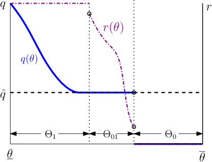
Figure 1: Graphical illustration of a floor randomized mechanism

Theorem 1

Any IC and IR mechanism that is not floor randomized is dominated by a floor randomized mechanism.

Thus, the set of undominated mechanisms is a subset of the set of floor randomized mechanisms. The proof of Theorem 1 is in Appendix A. To see the main idea behind this proof, consider a deterministic IC and IR mechanisms $M$ in which every type is allowed to operate and produces a strictly positive quantity $q^{\dagger}<\hat{q}$. Furthermore, assume that $u(\overline{\theta})=0$. Clearly, $M$ is not floor randomized. In its floor randomized transformation, $M^{T}$, every type is allowed to operate with probability $\frac{q^{\dagger}}{\hat{q}}$ and produces a quantity $\hat{q}$. We now argue that moving from deterministic operation to stochastic operation can make the regulator better off at every $\theta$. To see why, consider the difference

$$\textsc{RS}_{\alpha}(\theta,M^{T})-\textsc{RS}_{\alpha}(\theta,M) =\frac{q^{\dagger}}{\hat{q}}\Big{(}V(\hat{q})-c\Big{)}-\Big{(}V(q^{\dagger})-c\Big{)}$$

$$=\frac{q^{\dagger}}{\hat{q}}\widetilde{V}(\hat{q})+\left(1-\frac{q^{\dagger}}{\hat{q}}\right)\widetilde{V}(0)-\widetilde{V}(q^{\dagger})$$

where $\widetilde{V}(q)=\Big{(}V(q)-c\Big{)}\mathbf{1}_{\{q>0\}}$. If $\widetilde{V}(q)$ was a concave function, then Jensen’s inequality would have implied that the difference is negative. However, $\widetilde{V}(q)$ is not concave because of the discontinuity at $0$. Figure 2 plots $\widetilde{V}(q)$, and pictorially depicts both the terms in the difference. As can be seen, the expected value of $\widetilde{V}(q)$ is denoted by the ($\blacksquare$). On the other hand, the value of $\widetilde{V}(q^{\dagger})$ is denoted by ($\times$), and lies at a lower level. Thus, randomization is valuable to the regulator for quantities $q<\hat{q}$ as it reduces the occurrence of the fixed cost and simultaneously increases the value to the consumers relative to a deterministic mechanism.

Figure 2: Graphical illustration of $\widetilde{V}$

4 Undominated mechanisms

In this section, we provide a near-complete characterization of undominated mechanisms, and show that not every floor randomized mechanism is undominated. We begin by introducing a new deterministic IC and IR mechanism $M_{e}\equiv(q_{e},u_{e})$, where $u_{e}(\bar{\theta})=0$ and

$$P(q_{e}(\theta))=\theta~{}~{}~{}\textrm{or}~{}~{}~{}q_{e}(\theta)=P^{-1}(\theta)~{}\qquad~{}\forall~{}\theta.$$

Thus, the efficient quantity rule $q_{e}$ assigns every marginal cost $\theta$ the quantity that maximizes $\textsc{TS}(\theta,q)$. Because $P$ is strictly decreasing $q_{e}$ is single valued, positive, and strictly decreasing. Moreover, continuity and monotonicity of $P$ (assumption [A1]) ensures that $q_{e}$ is continuous. The next observation compares $q_{e}(\theta)$ to the quantity floor $\hat{q}$.

Observation 1

For every $\theta$, we have $q_{e}(\theta)>\hat{q}~{}~{}{\rm and}~{}~{}\textsc{TS}(\theta,\hat{q})>0$.

This observation, which is proven in Appendix B, states that the quantity floor is strictly below the efficient quantity for every type. We further partition the set of floor randomized mechanisms based on whether or not the quantity produced is weakly below the efficient quantity at all types.

Definition 3

A mechanism $(r,q,u)$ satisfies downward distortion (DD) if

$$q(\theta)\leq q_{e}(\theta)~{}\qquad~{}\forall~{}\theta$$

with an equality at $\underline{\theta}$. If the inequality is strict for every $\theta>\underline{\theta}$, then we say that mechanism $(r,q,u)$ satisfies strict downward distortion (strict DD).

As we establish later in this section, the quantity rule of every undominated mechanism will satisfy DD. In addition, undominated mechanisms must also be left continuous.

Definition 4

A mechanism $(r,q,u)$ is left continuous if the product $qr$ is left continuous.

Our next main results shows that undominated mechanisms satisfy downward distortion and left-continuity.

Theorem 2

Suppose $M\equiv(r,q,u)$ is an IC and IR mechanism. Then, the following statements are true:

1. If $M$ is undominated, then it is floor randomized, left continuous, and satisfies DD.

2. If $M$ is dominated, then it is dominated by a floor randomized and left-continuous mechanism satisfying DD.

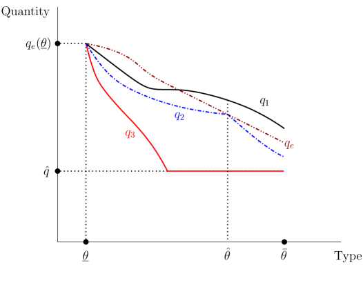
Figure 3: Illustration of necessary and sufficient conditions

Figure 3 plots quantity rules $q_{1},q_{2}$, and $q_{3}$ for three floor randomized mechanisms in which the monopolist always operates. The mechanism $M_{1}$ corresponding to the quantity rule $q_{1}$ violates DD, and by part (1) of Theorem 2, it is dominated. To see the intuition, consider another floor randomized mechanism $M\equiv(q,u)$ where $q(\theta)=\min\{q_{1}(\theta),q_{e}(\theta)\}$. For $\hat{\theta}$, which is shown in the figure, the total surplus is strictly larger under $M$ because $q(\theta)=q_{e}(\theta)<q_{1}(\theta)$. On the other hand, the rent paid to the monopolist is smaller because $q(\theta)\leq q_{1}(\theta)$ for all $\theta$. The proof in the Appendix B generalizes this intuition beyond deterministic floor randomized mechanisms. Moreover, it shows why left-continuity is also necessary.

Next, we show that strict DD, a stronger version of DD, and the remaining necessary conditions imply undomination.

Theorem 3

If a mechanism is floor randomized, left continuous, and satisfies strict DD, then it is undominated.

In Figure 3, the quantity rule $q_{2}$ satisfies DD but violates strict DD. Hence, Theorem 3 is silent whether the mechanism corresponding to $q_{2}$ is dominated or not. On the other hand the quantity rule $q_{3}$ satisfies strict DD and is left continuous. Hence, the corresponding floor randomized mechanism is undominated.

The proof of Theorem 3 is in Appendix B. Here, we discuss the role of strict DD in the proof. Consider a quantity rule $q$, which satisfies strict DD and corresponds to a deterministic floor randomized mechanism $M$. Such a $q$ is depicted in the Figure 4. The price-axis also plots the types, whereas the horizontal axis plots quantity. To show that $q$ is undominated, it must be that that any other mechanism cannot improve the regulator’s surplus at some type without lowering it at other types. In particular, the quantity rule $q_{1}$, which is obtained by lowering $q$ at some types, should not be able to improve the regulator’s surplus at $\hat{\theta}$. The rent saving corresponding to $q_{1}$ is given by $(1-\alpha)(A+B)$. Whereas the corresponding loss in the total surplus is given by $(B+C+D)$. The strict DD ensures that $D>0$, and therefore, even if $\alpha=0$ and area $A$ equals area $C$, the rent saving is always strictly smaller than the loss in the total surplus. Thus, $q_{1}$ can never dominate $q$.

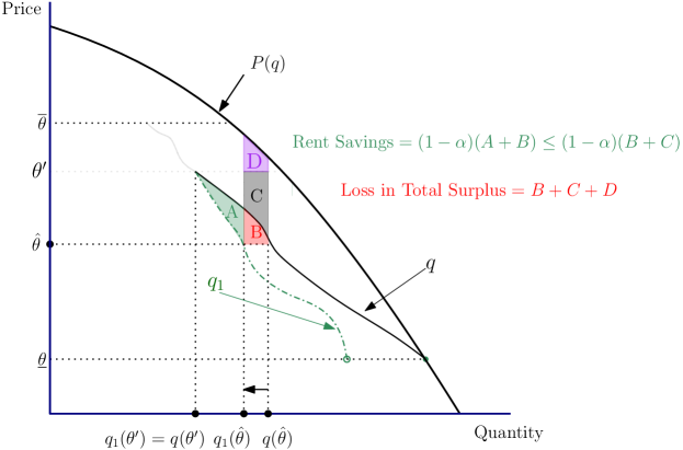
Figure 4: Strict DD and sufficiency

5 Implications for regulation

This section delves into the implications of our findings for regulatory design. First, it discusses why deterministic regulatory mechanisms are focal and identifies properties of optimal mechanisms (expected regulator surplus maximizing mechanism for a given prior) invariant to the details of the regulator’s prior. Then, it discusses the efficient mechanism. Finally, it identifies the max-min optimal mechanism for a regulator who entertains a set of priors over the marginal costs.

5.1 Deterministic regulatory mechanisms

In this section, we use the properties of undominated mechanisms stated in Theorem 1 and 2 to establish that focusing attention on deterministic mechanisms is without loss of generality in a certain sense. For every IC and IR mechanism $M$ and a prior $G$ over $\Theta$, define

$$\textsc{RS}_{\alpha}(M,G) =\int\limits_{\underline{\theta}}^{\bar{\theta}}\textsc{RS}_{\alpha}(\theta,M)dG(\theta).$$

We show the following.

Proposition 1

For every IC and IR mechanism $\widetilde{M}$ and every prior $G$ over $\Theta$, there exists a deterministic mechanism $M^{\star}$ such that

$$\textsc{RS}_{\alpha}(M^{\star},G) \geq\textsc{RS}_{\alpha}(\widetilde{M},G).$$

To prove this, fix an IC and IR mechanism $\widetilde{M}$ and a prior $G$. First, either $\widetilde{M}$ is undominated or by Theorem 2, there exists a mechanism $M$ that dominates $\widetilde{M}$ and is floor randomized. By Theorem 1, if $\widetilde{M}$ is undominated, it is also floor randomized. Hence, we conclude that there exists a floor randomized mechanism $M$ (where $M$ may be same as $\widetilde{M}$) such that

$$\textsc{RS}_{\alpha}(M,G) \geq\textsc{RS}_{\alpha}(\widetilde{M},G)$$ (5)

Now, let $M\equiv(r,q,u)$. Let $\mathcal{M}(q)$ be the set of all floor randomized mechanisms for the quantity rule $q$:

$$\mathcal{M}(q):=\{(r^{\dagger},q,u^{\dagger}):(r^{\dagger},q,u^{\dagger})~{}\textrm{is floor randomized}\}.$$

Clearly, $\mathcal{M}(q)$ is non empty because it contains $M$. In fact, it contains multiple elements when $q(\theta)=\hat{q}$ over an interval of $\theta$s. Observe that $\mathcal{M}(q)$ is a convex and compact set: if $(r^{\dagger},q,u^{\dagger})$ and $(r^{\ddagger},q,u^{\ddagger})$ are two mechanisms in $\mathcal{M}(q)$, their convex combination gives another floor randomized mechanism. Hence, by Krien-Milman theorem, the set $\mathcal{M}(q)$ is convex hull of its extreme points, where we define an extreme point as follows.

Definition 5

A mechanism $(r^{\dagger},q,u^{\dagger})\in\mathcal{M}(q)$ is an extreme point if there does not exist two other mechanisms $(r^{\prime},q,u^{\prime}),(r^{\prime\prime},q,u^{\prime\prime})\in\mathcal{M}(q)$ such that for some $\lambda\in(0,1)$

$$(r^{\dagger}(\theta),u^{\dagger}(\theta)) =\lambda(r^{\prime}(\theta),u^{\prime}(\theta))+(1-\lambda)(r^{\prime\prime}(\theta),u^{\prime\prime}(\theta))~{}\qquad~{}\forall~{}\theta\in\Theta.$$

The next lemma shows that every extreme point of $\mathcal{M}(q)$ is a deterministic mechanism.

Lemma 2

Every extreme point of $\mathcal{M}(q)$ is deterministic.

The proof of the above Lemma is similar to the proof of Lemma 4 in Manelli and Vincent (2007) and is given in Appendix C. It shows that any mechanism $(r,q,u)\in\mathcal{M}(q)$ involving randomization, that is $r(\theta)\in(0,1)$ for some $\theta$, can be written as a convex combination of two mechanisms in the set $\mathcal{M}(q)$.

Thus, any objective function that is linear in both $r$ and $u$ will attain its maximum at a deterministic mechanism. In particular, fixing $q$, consider the following objective function, which is linear in $(r,u)$.

$$\max_{(r,u)}\int\limits_{\Theta}\left(r(\theta)\textsc{TS}(\theta,q(\theta))-(1-\alpha)u(\theta)\right)dG(\theta),$$

As a result, Lemma 2 implies that a maximum over all $\mathcal{M}(q)$ can be achieved at a deterministic mechanism $M^{\star}$. Hence, there exists a deterministic mechanism $M^{\star}$ such that

$$\textsc{RS}_{\alpha}(M^{\star},G) \geq\textsc{RS}_{\alpha}(M,G),$$

where we used the fact that $M\in\mathcal{M}(q)$. Using (5), we get the desired inequality of Proposition 1. The pictorial depiction of the discussion so far is given in Figure 5.

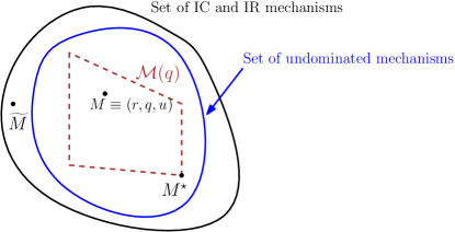
Figure 5: Pictorial depiction of Proposition 1

An important implication of Proposition 1 concerns optimal regulation design for a given prior. We say a mechanism $M^{\rm{OPT}}\equiv(r^{\rm{OPT}},q^{\rm{OPT}},u^{\rm{OPT}})$ is optimal for a prior $G$ over $\Theta$ if for every IC and IR mechanism $M$,

$$\textsc{RS}_{\alpha}(M^{\rm OPT},G) \geq\textsc{RS}_{\alpha}(M,G)$$

We say $M^{\rm{OPT}}$ has a quantity floor is $q^{\rm{OPT}}(\theta)\geq\hat{q}$ whenever $q^{\rm{OPT}}(\theta)>0$.

Corollary 1

For every prior $G$ over $\Theta$, there always exists a deterministic optimal mechanism for the prior $G$ that satisfies DD and has quantity floor.

The corollary follows from Proposition 1, which implies it is without loss of generality to focus attention on deterministic undominated mechanisms while searching for the optimal mechanism. The result follows because every undominated mechanism satisfies DD and has a quantity floor. Corollary 1 identifies properties of optimal mechanisms that are invariant to the regulator’s prior. Moreover, it does not require any assumptions on the regulator’s prior, and therefore, generalizes a finding of Baron and Myerson (1982), which states that for any distribution that admits positive density, the optimal mechanism is deterministic.

5.2 Efficient mechanism is dominated

Let $M_{e}\equiv(q_{e},u_{e})$ be a deterministic IC and IR mechanism in which each type $\theta$ produces quantity $q_{e}(\theta)$ and $u_{e}(\overline{\theta})=0$. We call $M_{e}$ the efficient mechanism. Clearly, the efficient mechanism is floor randomized because it is deterministic and $q_{e}(\theta)>\hat{q}$ for all $\theta$ (Observation 1). Moreover, it is continuous, and satisfies DD. However, it violates strict DD, and therefore, Theorem 3 is silent on whether $M_{e}$ is undominated. The next result shows that $M_{e}$ is dominated, no matter what $\alpha\in[0,1)$ is, when $P$ is twice continuously differentiable.

Theorem 4

If $P$ is twice continuously differentiable, then the efficient mechanism is dominated.

Theorem 4 highlights the limits of our necessary (Theorem 2) and sufficient (Theorem 3) conditions in identifying undominated mechanisms. It exhibits that some mechanisms satisfy the necessary conditions and are still dominated.

It is worth noting that if $\alpha=1$, equation (4) implies that the regulator’s surplus at type $\theta$ in a mechanism $(r,q,u)$ is $r(\theta)\textsc{TS}(\theta,q(\theta))$, which is uniquely maximized at $q_{e}(\theta)$ with $r(\theta)=1$. Therefore, $M_{e}$ is an undominated mechanism.

5.3 Max-min optimal mechanism

While the optimal mechanism design in Baron and Myerson (1982) fixes a prior and derives an optimal mechanism, the regulator may be ambiguity averse. To model this, let $\mathcal{F}$ denote the set of all probability distributions over $\Theta$. We assume that the regulator considers probability distributions in a set $\mathcal{G}\subseteq\mathcal{F}$ to be plausible. Suppose there exists $G^{\star}\in\mathcal{G}$ such that $G^{\star}\succ_{{\rm fosd}}G$ for every $G\in\mathcal{G}$, where $\succ_{{\rm fosd}}$ is the first-order stochastic domination relation. For example, if $\mathcal{G}=\mathcal{F}$, this assumption is automatically satisfied with $G^{\star}$ being the distribution that puts all the probability mass at $\bar{\theta}$. We solve for the max-min optimal mechanism for $\mathcal{G}$, where

Definition 6

An IC and IR mechanism $M$ is max-min optimal for $\mathcal{G}$ if for every IC and IR mechanism $M^{\prime}$

$$\inf_{G\in\mathcal{G}}\textsc{RS}_{\alpha}(M,G)\geq\inf_{G\in\mathcal{G}}\textsc{RS}_{\alpha}(M^{\prime},G).$$

Proposition 2

The optimal mechanism for prior $G^{\star}$ is max-min optimal for $\mathcal{G}$.

If we further assume that $G^{\star}$ admits a continuous and positive density, then the optimal mechanism for $G^{\star}$ is the Baron and Myerson (1982) optimal mechanism. Consequently, max-min optimal mechanism is the Baron and Myerson (1982) optimal mechanism for $G^{\star}$.

The proof of Proposition 2, which is given in Appendix C, is based on the following lemma, which is of independent interest. It shows that for any floor randomized mechanism satisfying DD, the expected regulator’s surplus for prior $G$ is higher than that for prior $G^{\prime}$, where $G^{\prime}\succ_{{\rm fosd}}G$. This lemma leverages the unique feature of floor randomized mechanisms that operation decisions are monotone functions.

Lemma 3

If $M\equiv(r,q,u)$ is a floor randomized mechanism that satisfies DD, then for all $G,G^{\prime}\in\mathcal{F}$ such that $G^{\prime}\succ_{{\rm fosd}}G$,

$$\textsc{RS}_{\alpha}(M,G)\geq\textsc{RS}_{\alpha}(M,G^{\prime}).$$

The proof of Lemma 3 is in Appendix C. If we treat a distribution in $\mathcal{F}$ as a “technology”, then $G^{\prime}\succ_{{\rm fosd}}G$ has the interpretation that $G$ is a better technology than $G^{\prime}$ (because $G$ puts more probability mass on lower marginal costs). A consequence of Lemma 3 is that as the technology gets better the regulator’s expected surplus improves from a floor randomized mechanism satisfying DD.

6 Related literature

There is an extensive theoretical literature on mechanism design approach to regulation. Armstrong and Sappington (2006) and Armstrong and Sappington (2004) are excellent surveys, where the latter provides a unified treatment of various results in the literature. We work in the model of Baron and Myerson (1982), which derives the optimal regulatory mechanism for a regulator who does not observe the marginal cost. The optimal regulatory mechanism depends on the prior. In contrast, our analysis is prior-free and seeks to understand undominated mechanisms.

While we, like Baron and Myerson (1982), assume that the inverse demand function is known to the regulator, Lewis and Sappington (1988a) analyzes a model where the regulator observes the cost function of the monopolist but not the inverse demand function. Lewis and Sappington (1988b); Armstrong (1999) analyze optimal regulatory mechanisms when the regulator does not know the cost and inverse demand functions.

A recent contribution by Guo and Shmaya (2024) analyzes robust regulatory mechanisms in a setup where the regulator does not know the inverse demand function or the monopolist’s cost function. In their paper, the regulator evaluates regulatory mechanisms by their worst-case regret, which is the difference between their complete information and the actual payoffs. They show that a price-cap mechanism is robustly optimal even in a setting where transfers are feasible. Our approach complements their analysis as it is also non-Bayesian but differs in the robustness criterion. Undomination, despite being a very weak robustness criterion, puts significant restrictions like floor randomization and downward distortion on the set of IC and IR mechanisms.

Undominated mechanism design has been studied in other models of mechanism design. For instance, in the multidimensional screening problem (where a monopolist is selling multiple goods to a buyer with multidimensional private values), Manelli and Vincent (2007) consider undominated selling mechanisms for the monopolist and show that they are optimal for some prior distribution over values of the buyer. Unlike us, they do not give necessary and sufficient conditions for a mechanism to be undominated.

For allocating a single object to multiple agents (with quasilinear utility), Sprumont (2013) characterizes undominated mechanisms in the class of strategy-proof, ex-post individually rational, feasible (weak budget-balance), anonymous, and envy-free mechanisms – see similar characterizations in Athanasiou and Valletta (2021) in the context of a public good problem. When selling multiple objects to a set of buyers who demand at most one object, Kazumura et al. (2020) show that a generalization of the Vickrey-Clarke-Groves (VCG) mechanism is the unique undominated mechanism among the class of strategy-proof and ex-post individually rational mechanisms satisfying no-subsidy, no-wastage, and equal treatment of equals. As is apparent, this literature focuses on settings with many agents and characterizes undominated mechanisms under additional constraints than IC and IR. A recent work by Borgers et al. (2024) analyze undominated mechanisms in a single object private values auction model, and shows that any second price auction with a positive reserve price is undominated.

As alluded in the introduction, an arbitrary IC and IR regulatory mechanism need not be monotonic, that is, the expected regulator surplus may reduce even when the distribution over marginal cost gets better as per first-order stochastic dominance relation. However, undominated regulatory mechanisms, as shown by our Lemma 3, are always monotone. This idea of considering monotone mechanisms (i.e., designer’s payoff increases as the prior distribution over the agent’s valuation gets better) was first introduced in the mechanism design literature by Hart and Reny (2015). They show that deterministic and symmetric IC mechanisms are monotone if the monopolist is selling multiple goods, but every IC mechanism is monotone if the monopolist is selling a single good.

Finally, our result on max-min optimal regulation contributes to the literature on robust mechanism design. This literature is reviewed in Carroll (2019) – also see Carroll (2017) who find a max-min optimal mechanism in the multidimensional screening model. A recent contribution by Bergemann et al. (2023) discusses max-min optimal procurement mechanisms for a government that evaluates a mechanism by the ratio of actual consumer surplus and its value in the complete information benchmark.

Appendix A Proofs of Section 3

Proof of Theorem 1. Let $M\equiv(r,q,u)$ be an IC and IR mechanism, and $M^{T}\equiv(r^{T},q^{T},u^{T})$ be its unique floor randomized transformation. Recall, for every $\theta$, we have $q^{T}(\theta)r^{T}(\theta)=q(\theta)r(\theta)$. Thus, using the notation $\overline{V}(q)=V(q)-c$, we can write

$$\textsc{RS}_{\alpha}(\theta,M^{T}) =r^{T}(\theta)\overline{V}(q^{T}(\theta))-\theta q^{T}(\theta)r^{T}(\theta)-(1-\alpha)u^{T}(\theta)$$

$$=r(\theta)\overline{V}(q(\theta))-\theta q(\theta)r(\theta)-(1-\alpha)\big{(}u(\theta)-u(\overline{\theta})\big{)}$$

$$\qquad+\Big{(}r^{T}(\theta)\overline{V}(q^{T}(\theta))-r(\theta)\overline{V}(q(\theta))\Big{)}$$

$$=\textsc{RS}_{\alpha}(\theta,M)+(1-\alpha)u(\overline{\theta})+\Big{(}r^{T}(\theta)\overline{V}(q^{T}(\theta))-r(\theta)\overline{V}(q(\theta))\Big{)}$$

Because $M$ is an IR mechanism, $u(\overline{\theta})\geq 0$, and therefore,

$$\textsc{RS}_{\alpha}(\theta,M^{T})-\textsc{RS}_{\alpha}(\theta,M) \geq r^{T}(\theta)\Big{(}V(q^{T}(\theta))-c\Big{)}-r(\theta)\Big{(}V(q(\theta))-c\Big{)}.$$ (6)

To complete the proof, it suffices to show that the RHS of inequality (6) is non-negative for all $\theta$, and it is positive for some $\theta$. Before we show that, consider the second term on the RHS of inequality (6). If $q(\theta)=0$, then $r(\theta)=0$, and therefore, the whole term is zero. Thus, this term can be thought of as a convex combination of points on the graph of the function $\widetilde{V}(q)=\big{(}V(q)-c\big{)}\mathbf{1}_{q>0}$. More formally, if $q(\theta)>0$, then

$$r(\theta)\Big{(}V(q(\theta))-c\Big{)}=r(\theta)\widetilde{V}(q(\theta))+(1-r(\theta))\widetilde{V}(0).$$

A similar interpretation also applied to the first term on the RHS. Thus, to evaluate the RHS of inequality (6), we need to consider the concave closure of $\widetilde{V}(q)$, which is the smallest concave function weakly above $\widetilde{V}$.

Observe $\widetilde{V}(q)$ is strictly increasing and strictly concave for all $0<q<\bar{q}$, where $\bar{q}$ is the unique $q$ such that $P(q)=0$. This is because the derivative of $\widetilde{V}(q)$ at $q>0$ is $P(q)$ which is positive and strictly decreasing. However, $\widetilde{V}$ has a discontinuity at $q=0$ because $\widetilde{V}(0)=0$ and $\lim_{q\downarrow 0}\widetilde{V}(q)=-c$. This means that $\widetilde{V}$ is not concave. The concave closure of function $\widetilde{V}$ is denoted by $co(\widetilde{V})$ and is given by

$$co(\widetilde{V})(q)=\begin{cases}qP(\hat{q})=\frac{\overline{V}(\hat{q})}{\hat{q}}q&\textrm{if}\ q<\hat{q}\\ \overline{V}(q)&\textrm{if}\ q\geq\hat{q}\end{cases}$$

Since $\hat{q}$ is such that $\overline{V}(\hat{q})=\hat{q}P(\hat{q})$, it follows that $co(\widetilde{V})$ defines the concave envelope of $\widetilde{V}$. Thus, $co(\widetilde{V})(q)$ is linearly increasing in $q$ till $\hat{q}$. For $q\geq\hat{q}$, $co(\widetilde{V})(q)$ is strictly concave and equals $\overline{V}(q)$. Figure 2 in the main text graphically illustrates $co(\widetilde{V})$.

Pick $\theta\in\Theta$. If $q(\theta)r(\theta)=0$, then the regulator’s surplus is identical under both $M$ and $M^{T}$. Below, we consider two cases and argue that the RHS of the inequality (6) is non-negative for all $\theta$.

Case 1. Let $\theta$ be such that $q(\theta)r(\theta)\geq\hat{q}$. Hence, by definition $r^{T}(\theta)=1$ and $q^{T}(\theta)=q(\theta)r(\theta)$. Then,

$$\textsc{RS}_{\alpha}(\theta,M^{T})-\textsc{RS}_{\alpha}(\theta,M) \geq r^{T}(\theta)\overline{V}(q^{T}(\theta))-r(\theta)\overline{V}(q(\theta))$$

$$=co(\widetilde{V})(q(\theta)r(\theta))-r(\theta)co(\widetilde{V})(q(\theta))$$

$$\geq 0$$

where the inequality follows from concavity of $co(\widetilde{V})$ and $co(\widetilde{V})(0)=0$. If $r(\theta)<1$, then inequality is strict because of the strict concavity of $co(\widetilde{V})$ on $q\geq\hat{q}$.

Case 2. Let $\theta$ be such that $0<q(\theta)r(\theta)<\hat{q}$. Then, $q^{T}(\theta)=\hat{q}$ and $r^{T}(\theta)=\frac{q(\theta)r(\theta)}{\hat{q}}$. Moreover,

$$\textsc{RS}_{\alpha}(\theta,M^{T})-\textsc{RS}_{\alpha}(\theta,M) \geq r^{T}(\theta)\overline{V}(q^{T}(\theta))-r(\theta)\overline{V}(q(\theta))$$

$$=\frac{q(\theta)r(\theta)}{\hat{q}}\overline{V}(\hat{q})-r(\theta)\overline{V}(q(\theta))$$

$$=co(\widetilde{V})(q(\theta)r(\theta))-r(\theta)\overline{V}(q(\theta))$$

$$\geq co(\widetilde{V})(q(\theta)r(\theta))-r(\theta)co(\widetilde{V})(q(\theta))$$

$$\geq 0$$

where the second equality follows from the definition of $co(\widetilde{V})$, the second inequality follows because $co(\widetilde{V})(q)\geq\overline{V}(q)$ for all $q$, and the last inequality follows from concavity of $co(\widetilde{V})$ and $co(\widetilde{V})(0)=0$. If $q(\theta)\neq\hat{q}$, this inequality is strict.

To complete the proof, observe that $M$ is not floor randomized, and therefore, we must have at least one $\theta$ where $q(\theta)r(\theta)\geq\hat{q}$ but $r(\theta)<1$ or $0<q(\theta)r(\theta)\leq\hat{q}$ and $q(\theta)\neq\hat{q}$. That is, the RHS of inequality (6) is positive at this $\theta$. $\blacksquare{}$

Appendix B Proofs of Section 4

Proof of Observation 1. Let $\Delta(q)=\overline{V}(q)-P(q)q$. Notice that $\Delta(q)$ is strictly increasing and continuous in $q$ as $\Delta^{\prime}(q)=-P^{\prime}(q)q>0$. Further, by definition of $\hat{q}$, we have $\Delta(\hat{q})=0$. Now,

$$\Delta(q_{e}(\bar{\theta})) =\overline{V}(P^{-1}(\bar{\theta}))-\bar{\theta}P^{-1}(\bar{\theta})>0,$$

where the inequality follows from assumption $[A2]$. By continuity and monotonicity of $\Delta$, we have $\hat{q}<q_{e}(\overline{\theta})$. This further implies $\hat{q}<q_{e}(\theta)$ for all $\theta$ because $q_{e}$ decreases in $\theta$. Finally, consider

$$\textsc{TS}(\theta,\hat{q})=\overline{V}(\hat{q})-\theta\hat{q}\geq\overline{V}(\hat{q})-\overline{\theta}\hat{q}=\big{(}P(\hat{q})-\overline{\theta}\big{)}\hat{q}>0,$$

where the last inequality holds because $\hat{q}<q_{e}(\overline{\theta})$ and $P(\cdot)$ is strictly decreasing. $\blacksquare{}$

Proof of Theorem 2. Suppose $M$ is undominated. By Theorem 1, it is floor randomized. Lemma 4 and Lemma 5, which are stated and proved below, establish that a floor randomized mechanism violating DD or left-continuity is dominated. Thus, completing the proof of Part 1.

As for Part 2, consider a dominated IC and IR mechanism $M$, which is not floor randomized. By Theorem 1, $M$ is dominated by its floor randomized transformation $M^{T}$. We can further use Lemma 4 and Lemma 5 to transform $M^{T}$ into another floor randomized mechanism $\widetilde{M}$ that dominates $M$ and satisfies DD and left-continuity. $\blacksquare{}$

Lemma 4

Suppose $M\equiv(r,q,u)$ is a floor randomized mechanism. Then, there exists a floor randomized mechanism $\widetilde{M}\equiv(\tilde{r},\tilde{q},\tilde{u})$ satisfying DD such that

$$\tilde{q}(\theta) \leq q(\theta) \forall~{}\theta>\underline{\theta}$$ (7)

$$\tilde{u}(\theta) \leq u(\theta) \forall~{}\theta$$

$$\textsc{RS}_{\alpha}(\theta,\widetilde{M}) \geq\textsc{RS}_{\alpha}(\theta,M) \forall~{}\theta$$ (8)

Inequalities (7) and (8) are strict for all $\theta$ where $M$ violates DD.

Proof. Define a new quantity rule $\tilde{q}$ as follows

$$\tilde{q}(\theta) :=\begin{cases}q_{e}(\theta)&\textrm{if $\theta=\underline{\theta}$ or $q(\theta)>q_{e}(\theta)$}\\ q(\theta)&\textrm{otherwise}\end{cases}$$

Consider mechanism $\widetilde{M}=(\tilde{r},\tilde{q},\tilde{u})$, where $\tilde{r}(\underline{\theta})=1$ and $\tilde{r}(\theta)=r(\theta)$ for all $\theta\neq\underline{\theta}$. Moreover,

$$\tilde{u}(\theta) :=\int\limits_{\theta}^{\overline{\theta}}\tilde{q}(y)\tilde{r}(y)dy~{}\qquad~{}\forall~{}\theta.$$ (9)

Both $q$ and $r$ are decreasing in $\theta$ because $M$ is a floor randomized mechanism. Moreover, $q_{e}$ also decreases in $\theta$. Thus, $\tilde{q}$ as well as $\tilde{r}$ decrease in $\theta$. Monotonicity of $\tilde{q}(\theta)\tilde{r}(\theta)$ in $\theta$ along with equation (9) implies $\widetilde{M}$ is IC. It is also IR with $\tilde{u}(\overline{\theta})=0$. To see why $\widetilde{M}$ is a floor randomized mechanisms, consider the following two cases.
case 1. Suppose $\Theta^{M}_{1}=\emptyset$. In this case, $q(\theta)\in\{0,\hat{q}\}$ for all $\theta$. Thus, $\tilde{q}$ differs from $q$ only at $\underline{\theta}$, implying that $\Theta^{\widetilde{M}}_{1}=\{\underline{\theta}\}$. Furthermore,

$$\Theta^{\widetilde{M}}_{01} =\begin{cases}\Theta^{M}_{01}&\textrm{if $\Theta_{01}^{M}=\emptyset$}\\ \Theta^{M}_{01}\setminus\{\underline{\theta}\}&\textrm{otherwise}\end{cases} \Theta^{\widetilde{M}}_{0} =\begin{cases}\Theta^{M}_{0}\setminus\{\underline{\theta}\}&\textrm{if $\Theta^{M}_{01}=\emptyset$}\\ \Theta^{M}_{0}&\textrm{otherwise}\end{cases}$$

case 2. If $\Theta^{M}_{1}\neq\emptyset$, then $\tilde{q}$ differs from $q$ only on a subset of $\Theta^{M}_{1}$. For every $\theta$ in this subset, $\tilde{q}(\theta)=q_{e}(\theta)>\hat{q}$, and therefore, $\tilde{r}(\theta)=1$. Consequently,

$$\Theta^{\widetilde{M}}_{1} =\Theta^{M}_{1} \Theta^{\widetilde{M}}_{01} =\Theta^{M}_{01} \Theta^{\widetilde{M}}_{0} =\Theta^{M}_{0}.$$

We now argue that mechanism $\widetilde{M}$ satisfies DD and all the relevant inequalities in the statement of Lemma 4 hold. Observe that $\tilde{q}(\theta)\leq\min\{q_{e}(\theta),q(\theta)\}$ for all $\theta$, and thus, $\tilde{q}(\theta)$ satisfies DD. Moreover, $\tilde{q}(\theta)\leq q(\theta)$ for all $\theta$ with a strict inequality where $q$ violates DD. We also have

$$\tilde{u}(\theta)=\int\limits_{\theta}^{\overline{\theta}}\tilde{q}(y)\tilde{r}(y)dy\leq\int\limits_{\theta}^{\overline{\theta}}q(y)r(y)dy=u(\theta)\qquad\forall~{}\theta.$$

Thus, to complete the proof it suffice to show that the total surplus under $\widetilde{M}$ is larger than that under $M$ at every $\theta$. Total surplus is unchanged for $\theta$ if $\theta\neq\underline{\theta}$ and $q(\theta)\leq q_{e}(\theta)$. For $\theta$ such that $\theta=\underline{\theta}$ or $q(\theta)>q_{e}(\theta)$, we have $\tilde{q}(\theta)=q_{e}(\theta)$. By definition of $q_{e}$, total surplus is higher in $\widetilde{M}$ than in $M$. $\blacksquare{}$

Lemma 5

Suppose $M\equiv(r,q,u)$ is a floor randomized mechanism satisfying DD. Then, there exists another floor randomized mechanism $\widetilde{M}\equiv(\tilde{r},\tilde{q},u)$ satisfying DD and left-continuity such that

$$\tilde{q}(\theta)\tilde{r}(\theta) \geq q(\theta)r(\theta) \forall~{}\theta$$

$$\textsc{CS}(\theta,\widetilde{M}) \geq\textsc{CS}(\theta,M) \forall~{}\theta$$

$$\textsc{RS}_{\alpha}(\theta,\widetilde{M}) \geq\textsc{RS}_{\alpha}(\theta,M) \forall~{}\theta$$

with equality holding for almost all $\theta$. Moreover, the above inequalities are strict at $\theta$s where $M$ violates left-continuity.

Proof. Because $q(\theta)r(\theta)$ is decreasing, it violates left-continuity at countably many types. Let $\Theta_{d}$ be the set of such types. We modify $q$ and $r$ at these types to obtain a new quantity rule $\tilde{q}$ and a new operation decision $\tilde{r}$.

$$\tilde{q}(\theta) =\lim_{z\uparrow\theta}q(z) \tilde{r}(\theta) =\lim_{z\uparrow\theta}r(z) \forall~{}\theta\in\Theta_{d}$$

By construction, $\tilde{q}\tilde{r}$ is left continuous at all $\theta\in\Theta_{d}$, and as a result, it is also left continuous at all $\theta$. Therefore, the IC and IR mechanism $\widetilde{M}\equiv(\tilde{r},\tilde{q},\tilde{u})$, where $\tilde{u}(\theta)=\int\limits_{\theta}^{\overline{\theta}}\tilde{q}(y)\tilde{r}(y)dy$, is also left continuous. Moreover, $\widetilde{M}$ is floor randomized and satisfies DD because $M$ satisfies both these properties. Below, we argue that $\widetilde{M}$ dominates $M$.

For mechanism $\widetilde{M}$, the regulator’s surplus at any type $\theta$ is

$$\tilde{r}(\theta)\textsc{TS}(\theta,\tilde{q}(\theta))-(1-\alpha)\tilde{u}(\theta).$$

Because $\tilde{q}(\theta)\tilde{r}(\theta)$ differs from $q(\theta)r(\theta)$ on measure zero types, we have $\tilde{u}(\theta)=u(\theta)$ for all $\theta$. Thus, it is enough to show that

$$\tilde{r}(\theta)\textsc{TS}(\theta,\tilde{q}(\theta))>r(\theta)\textsc{TS}(\theta,q(\theta))~{}~{}\forall~{}\theta\in\Theta_{d}$$

Fix $\theta\in\Theta_{d}$. First, suppose that $r(\theta)=0$. Then, $q(\theta)=0$. However, $\tilde{q}(\theta)\tilde{r}(\theta)>0$. Otherwise, $qr$ will be continuous at $\theta$, a contradiction. In particular, we have $\tilde{q}(\theta)>0$ and $\tilde{r}(\theta)>0$, and a larger expected total surplus under $\widetilde{M}$ at $\theta$. To complete the proof, consider the remaining case where $r(\theta)>0$. Because $M$ is floor randomized, $q(\theta)\geq\hat{q}$. Moreover, by construction, either $\tilde{q}(\theta)>q(\theta)$ or $\tilde{r}(\theta)>r(\theta)$. Because both $M$ and $\widetilde{M}$ satisfy DD, the increase in quantity or probability of operation increases the expected total surplus at $\theta$. $\blacksquare{}$

Proof of Theorem 3. Suppose $M\equiv(q,r,u)$ is a floor randomized, left-continuous mechanism that satisfies strict DD. By contradiction, assume $M$ is dominated by another mechanism $\widetilde{M}\equiv(\tilde{r},\tilde{q},\tilde{u})$. Part (2) of Theorem 2 implies that we can find $\widetilde{M}$ such that it is floor randomized, left continuous, and satisfies DD. Let

$$D_{qr} :=\{\theta:\tilde{q}(\theta)\tilde{r}(\theta)<q(\theta)r(\theta)\}.$$

By Lemma 6, $D_{qr}$ has a positive measure. Next, define

$$\theta_{h} :=\sup~{}\{\theta:\theta\in D_{qr}\}.$$

$\theta_{h}$ is a finite real number because $D_{qr}$ is non-empty and bounded. Clearly, $\theta_{h}>\underline{\theta}$. In what follows, the proof obtains a contradiction by showing that there exists $\theta$, in a left neighbourhood of $\theta_{h}$, at which the regulator gets a higher surplus under mechanism $M$. To do so, it considers two cases: 1) $r(\theta_{h})\in[0,1)$, and 2) $r(\theta_{h})=1$.

Case 1. If $r(\theta_{h})\in[0,1)$, then $q(\theta_{h})r(\theta_{h})<\hat{q}$ (since $M$ is a floor randomized mechanism). There exists $\theta_{\ell}<\theta_{h}$, along with a corresponding left-neighbourhood $\mathcal{N}:=[\theta_{\ell},\theta_{h})$ of $\theta_{h}$, such that

$$\hat{q}>_{(a)}q(\theta)r(\theta)>_{(b)}\tilde{q}(\theta)\tilde{r}(\theta)\geq 0~{}\qquad~{}\forall~{}\theta\in\mathcal{N}.$$

Inequality $(a)$ holds because $qr$ is decreasing in $\theta$ and left continuous at $\theta_{h}$. As for inequality $(b)$, it follows from the definition of $\theta_{h}$. Thus, for every $\theta\in\mathcal{N}$, we have $q(\theta)=\hat{q}$ and $r(\theta)>0$. Furthermore, $r(\theta)>\tilde{r}(\theta)$. To see why, notice that $\hat{q}r(\theta)>\tilde{q}(\theta)\tilde{r}(\theta)$ and $\widetilde{M}$ being floor randomized imply $\tilde{q}(\theta)\in\{0,\hat{q}\}$. In both these cases, inequality $(b)$ implies $r(\theta)>\tilde{r}(\theta)$. Now, let

$$\Delta:=\sup_{y\in\mathcal{N}}r(y)-\tilde{r}(y),$$

which is a strictly positive. Thus, there exists $\theta\in\mathcal{N}$ such that $r(\theta)-\tilde{r}(\theta)=\Delta-\epsilon$, where $\epsilon<\Delta\frac{P(\hat{q})-P(q_{e}(\overline{\theta}))}{P(\hat{q})-P(q_{e}(\underline{\theta}))}$. Consider the difference

$$\textsc{RS}_{\alpha}(\theta,M)-\textsc{RS}_{\alpha}(\theta,\widetilde{M}) =~{}~{}~{}r(\theta)\big{(}\overline{V}(\hat{q})-\theta\hat{q}\big{)}-\tilde{r}(\theta)\big{(}\overline{V}(\tilde{q}(\theta))-\theta\hat{q}\big{)}-(1-\alpha)\big{(}u(\theta)-\tilde{u}(\theta)\big{)}$$

$$\geq_{(a)}\Big{(}r(\theta)-\tilde{r}(\theta)\Big{)}\big{(}\overline{V}(\hat{q})-\theta\hat{q}\big{)}-(1-\alpha)\big{(}u(\theta)-\tilde{u}(\theta)\big{)}$$

$$=_{(b)}\Big{(}r(\theta)-\tilde{r}(\theta)\Big{)}\hat{q}\big{(}P(\hat{q})-\theta\big{)}-(1-\alpha)\big{(}u(\theta)-\tilde{u}(\theta)\big{)}$$

where inequality $(a)$ follows from $\tilde{q}(\theta)\in\{0,\hat{q}\}$. As for equality $(b)$, it uses the fact that $\overline{V}(\hat{q})=\hat{q}P(\hat{q})$. To reach a contradiction and complete the proof, it suffices to show that the right hand side of the above equation is positive.

$$\Big{(}r(\theta)-\tilde{r}(\theta)\Big{)}\hat{q}\big{(}P(\hat{q})-\theta\big{)}-(1-\alpha)\big{(}u(\theta)-\tilde{u}(\theta)\big{)}$$

$$=\Big{(}r(\theta)-\tilde{r}(\theta)\Big{)}\hat{q}\big{(}P(\hat{q})-\theta\big{)}-(1-\alpha)\Big{(}\hat{q}\int\limits_{\theta}^{\theta_{h}}\big{(}r(y)-\tilde{r}(y)\big{)}dy\Big{)}-(1-\alpha)\Big{(}\int\limits_{\theta_{h}}^{\overline{\theta}}\big{(}q(y)r(y)-\tilde{q}(y)\tilde{r}(y)\big{)}dy\Big{)}$$

(since $$r(y)>\tilde{r}(y)\geq 0 y\in[\theta,\theta_{h} u(\overline{\theta})=\tilde{u}(\overline{\theta})=0$$ for all ) and )

$$\geq\Big{(}r(\theta)-\tilde{r}(\theta)\Big{)}\hat{q}\big{(}P(\hat{q})-\theta\big{)}-(1-\alpha)\Big{(}\hat{q}\int\limits_{\theta}^{\theta_{h}}\big{(}r(y)-\tilde{r}(y)\big{)}dy\Big{)}$$

(since $$q(y)r(y)\leq\tilde{q}(y)\tilde{r}(y) y>\theta_{h}$$ for all )

$$\geq\Big{(}r(\theta)-\tilde{r}(\theta)\Big{)}\hat{q}\big{(}P(\hat{q})-\theta\big{)}-\Big{(}\hat{q}\int\limits_{\theta}^{\theta_{h}}\big{(}r(y)-\tilde{r}(y)\big{)}dy\Big{)}~{}\qquad~{}\textrm{(since $r(y)>\tilde{r}(y)$ for all $y\in[\theta,\theta_{h})$)}$$

$$\geq\Big{(}r(\theta)-\tilde{r}(\theta)\Big{)}\hat{q}\big{(}P(\hat{q})-\theta\big{)}-\hat{q}\Delta(\theta_{h}-\theta)$$

$$=(\Delta-\epsilon)\hat{q}\big{(}P(\hat{q})-\theta\big{)}-\hat{q}\Delta(\theta_{h}-\theta)$$

$$=\Delta\hat{q}\big{(}P(\hat{q})-\theta_{h})-\epsilon\hat{q}\big{(}P(\hat{q})-\theta\big{)}$$

$$\geq\Delta\hat{q}\big{(}P(\hat{q})-\bar{\theta})-\epsilon\hat{q}\big{(}P(\hat{q})-\underline{\theta}\big{)}$$

$$=\Delta\hat{q}\big{(}P(\hat{q})-P(q_{e}(\bar{\theta}))\big{)}-\epsilon\hat{q}\big{(}P(\hat{q})-P(q_{e}(\underline{\theta}))\big{)}$$

$$>0$$

where the last inequality follows from Lemma 1 ($\hat{q}<q_{e}(\bar{\theta})$) and the fact that $\epsilon<\Delta\frac{P(\hat{q})-P(q_{e}(\overline{\theta}))}{P(\hat{q})-P(q_{e}(\underline{\theta}))}$.

Case 2. Suppose $r(\theta_{h})=1$. Then, by Lemma 7, $\tilde{r}(\theta_{h})=1$. Because both $M$ and $\widetilde{M}$ are floor randomized, $r(\theta)=\tilde{r}(\theta)=1$ for all $\theta\leq\theta_{h}$. Therefore, it suffices to focus on $q$ and $\tilde{q}$, which are left continuous on $\theta\leq\theta_{h}$, for comparing the regulator’s surplus for types below $\theta_{h}$.

There exists a non-empty left-neighbourhood $\mathcal{N}:=[\theta_{l},\theta_{h})$ of $\theta_{h}$ such that

$$\tilde{q}(\theta)<_{(a)}q(\theta)<_{(b)}q_{e}(\theta_{h})~{}\forall~{}\theta\in\mathcal{N}.$$

Inequality $(a)$ holds because of the definition of $\theta_{h}$. Whereas, inequality $(b)$ is guaranteed because $q(\theta_{h})<q_{e}(\theta_{h})$ ($M$ satisfies strict DD) and $q$ is left continuous and decreasing. Let

$$\Delta=\sup_{y\in\mathcal{N}}q(y)-\tilde{q}(y),$$

which is strictly positive. Thus, there exists $\theta\in\mathcal{N}$ such that $q(\theta)-\tilde{q}(\theta)=\Delta-\epsilon$, where $\epsilon<\Delta\frac{P(q(\theta_{l}))-P(q_{e}(\theta_{h}))}{P(q(\theta_{l}))-P(q_{e}(\underline{\theta}))}$. Now, consider the difference

$$\textsc{RS}_{\alpha}(\theta,M)-\textsc{RS}_{\alpha}(\theta,\widetilde{M}) =\int\limits_{\tilde{q}(\theta)}^{q(\theta)}\big{(}P(z)-\theta\big{)}dz-(1-\alpha)\big{(}u(\theta)-\tilde{u}(\theta)\big{)}.$$

To reach a contradiction and complete the proof, it suffices to show that the right hand side of the above equation is positive.

$$\int\limits_{\tilde{q}(\theta)}^{q(\theta)}\big{(}P(z)-\theta\big{)}dz-(1-\alpha)\Big{(}u(\theta)-\tilde{u}(\theta)\Big{)}$$

$$=\int\limits_{\tilde{q}(\theta)}^{q(\theta)}\big{(}P(z)-\theta\big{)}dz-(1-\alpha)\Big{(}\int\limits_{\theta}^{\theta_{h}}\big{(}q(y)-\tilde{q}(y)\big{)}dy\Big{)}$$

$$\qquad-(1-\alpha)\Big{(}\int\limits_{\theta_{h}}^{\overline{\theta}}\big{(}q(y)r(y)-\tilde{q}(y)\tilde{r}(y)\big{)}dy\Big{)} u(\overline{\theta})=0 \tilde{u}(\overline{\theta})=0$$ (since and )

$$\geq\int\limits_{\tilde{q}(\theta)}^{q(\theta)}\big{(}P(z)-\theta\big{)}dz-(1-\alpha)\Big{(}\int\limits_{\theta}^{\theta_{h}}\big{(}q(y)-\tilde{q}(y)\big{)}dy\Big{)} q(y)r(y)\leq\tilde{q}(y)\tilde{r}(y) y>\theta_{h}$$ (since for all )

$$\geq\int\limits_{\tilde{q}(\theta)}^{q(\theta)}\big{(}P(z)-\theta\big{)}dz-\int\limits_{\theta}^{\theta_{h}}\big{(}q(y)-\tilde{q}(y)\big{)}dy q(y)>\tilde{q}(y) y\in[\theta,\theta_{h})$$ (since for all )

$$\geq\big{(}P(q(\theta_{\ell}))-\theta\big{)}(q(\theta)-\tilde{q}(\theta))-\Delta(\theta_{h}-\theta) q(\theta_{\ell})\geq q(\theta) \Delta$$ (since and by definition of )

$$=\big{(}P(q(\theta_{\ell}))-\theta\big{)}(\Delta-\epsilon)-\Delta(\theta_{h}-\theta)$$

$$=\Delta\big{(}P(q(\theta_{\ell}))-\theta_{h}\big{)}-\epsilon\big{(}P(q(\theta_{\ell}))-\theta\big{)}$$

$$\geq\Delta\big{(}P(q(\theta_{\ell}))-\theta_{h}\big{)}-\epsilon\big{(}P(q(\theta_{\ell}))-\underline{\theta}\big{)}$$

$$>0$$

where the last inequality follows from $\epsilon<\Delta\frac{P(q(\theta_{l}))-P(q_{e}(\theta_{h}))}{P(q(\theta_{l}))-P(q_{e}(\underline{\theta}))}$. $\blacksquare{}$

Lemma 6

The set $D_{qr}$ has a positive measure.

Proof. Both $M$ and $\widetilde{M}$ satisfy DD, and therefore, $q(\underline{\theta})=\tilde{q}(\underline{\theta})=q_{e}(\underline{\theta})$. Thus, the total surplus from both the mechanisms at $\underline{\theta}$ is the same. Because $\widetilde{M}$ dominates $M$, it must be that the rent paid by the monopolist of type $\underline{\theta}$ is lower in $\widetilde{M}$ than in $M$, that is,

$$u(\underline{\theta})=\int\limits_{\underline{\theta}}^{\bar{\theta}}q(z)r(z)dz\geq\int\limits_{\underline{\theta}}^{\bar{\theta}}\tilde{q}(z)\tilde{r}(z)dz=\tilde{u}(\underline{\theta}).$$ (10)

If the inequality is an equality, $q(\theta)r(\theta)=\tilde{q}(\theta)\tilde{r}(\theta)$ for almost all $\theta$, and by left-continuity of $M$ and $\widetilde{M}$, $q(\theta)r(\theta)=\tilde{q}(\theta)\tilde{r}(\theta)$ for all $\theta$. Because both $M$ and $\widetilde{M}$ are floor randomized mechanisms, this implies $M=\widetilde{M}$, which is a contradiction. Thus, inequality (10) is strict, and $q(\theta)r(\theta)>\tilde{q}(\theta)\tilde{r}(\theta)$ for a positive measure of $\theta$. Consequently, $D_{qr}$ has a positive measure. $\blacksquare{}$

Lemma 7

If $r(\theta_{h})=1$, then $\tilde{r}(\theta_{h})=1$ and $q(\theta_{h})=\tilde{q}(\theta_{h})$.

Proof. For all $\theta>\theta_{h}$, we have $q(\theta)r(\theta)\leq\tilde{q}(\theta)\tilde{r}(\theta)$. Therefore, the rent paid by the monopolist of type $\theta_{h}$ is lower in $M$ than in $\widetilde{M}$, that is $u(\theta_{h})\leq\tilde{u}(\theta_{h})$. It must be that the expected total surplus is higher in $\widetilde{M}$ than $M$ at $\theta_{h}$:

$$\tilde{r}(\theta_{h})\Big{(}\overline{V}(\tilde{q}(\theta_{h}))-\theta_{h}\tilde{q}(\theta_{h})\Big{)}\geq r(\theta_{h})\Big{(}\overline{V}(q(\theta_{h}))-\theta_{h}q(\theta_{h})\Big{)}$$ (11)

Otherwise, $\widetilde{M}$ cannot dominate $M$ at $\theta_{h}$, a contradiction. We now use this inequality to show the desired result.

Suppose $r(\theta_{h})=1$. In this case, $q(\theta_{h})\geq\tilde{r}(\theta_{h})\tilde{q}(\theta_{h})$. If $\tilde{r}(\theta_{h})=1$, then $q(\theta_{h})\geq\tilde{q}(\theta_{h})$. Else, $\tilde{q}(\theta_{h})\leq\hat{q}\leq q(\theta_{h})$. In both these cases, we have $q(\theta_{h})\geq\tilde{q}(\theta_{h})$. Thus,

$$\tilde{r}(\theta_{h})\Big{(}\overline{V}(\tilde{q}(\theta_{h}))-\theta_{h}\tilde{q}(\theta_{h})\Big{)} \leq\Big{(}\overline{V}(\tilde{q}(\theta_{h}))-\theta_{h}\tilde{q}(\theta_{h})\Big{)}$$

$$\leq\Big{(}\overline{V}(q(\theta_{h}))-\theta_{h}q(\theta_{h})\Big{)}$$

$$=r(\theta_{h})\Big{(}\overline{V}(q(\theta_{h}))-\theta_{h}q(\theta_{h})\Big{)}$$

Using equation (11), we conclude that $\tilde{r}(\theta_{h})=1$ and $q(\theta_{h})=\tilde{q}(\theta_{h})$. $\blacksquare{}$

Appendix C Proofs of Section 5

Proof of Lemma 2. Let $(r,q,u)\in\mathcal{M}(q)$ be such that $r(\theta)\in(0,1)$ for some $\theta$. It suffices to show that $(r,q,u)$ is not an extreme point of $\mathcal{M}(q)$. That is, it is enough to establish that there exists two decreasing functions $\hat{r}$ and $\tilde{r}$, both taking values in $[0,1]$, and satisfying

$$r(\theta)=\frac{1}{2}\hat{r}(\theta)+\frac{1}{2}\tilde{r}(\theta)~{}~{}\forall~{}\theta.$$

Notice that the above equation, in combination with $q,$ will then imply $u=\frac{1}{2}\hat{u}(\theta)+\frac{1}{2}\tilde{u}(\theta)$, establishing that $(r,q,u)$ can be written as convex combination of two mechanism, $(\hat{r},q,\hat{u})$ and $(\tilde{r},q,\tilde{u})$, both in $\mathcal{M}(q)$.

To do so, consider

$$\hat{r}(\theta)=\begin{cases}0&\textrm{if}~{}r(\theta)<0.5\\ 2r(\theta)-1&\textrm{if}~{}r(\theta)\geq 0.5\end{cases}\hskip 36.135pt\tilde{r}(\theta)=\begin{cases}2r(\theta)&\textrm{if}~{}r(\theta)<0.5\\ 1&\textrm{if}~{}r(\theta)\geq 0.5\end{cases}$$

It is easy to see that $r(\theta)=\frac{1}{2}(\hat{r}(\theta)+\tilde{r}(\theta))$ for all $\theta$. Both $\hat{r}$ and $\tilde{r}$ are feasible, that is, they take values in $[0,1]$. Finally, both $\hat{r}$ and $\tilde{r}$ are decreasing because $r$ is decreasing. If $r(\theta)\notin\{0,1\}$ for some $\theta$, then $\hat{r}(\theta)\neq\tilde{r}(\theta)$. Therefore, $r$ can be written as convex combination of two more decreasing functions. $\blacksquare{}$

Proof of Theorem 4. Let $Q=[q_{e}(\overline{\theta}),q_{e}(\underline{\theta})]$. We begin by arguing that there exists an interval $[q_{0},q_{1}]\subset Q$ on which $P$ is either concave or convex. If $P^{\prime\prime}(q)=0$ for all $q\in Q$, then any closed interval contained in $Q$ is the desired interval. Otherwise, $P^{\prime\prime}(q)\neq 0$ for some $q$. By continuity of the second derivative, we can find a closed interval $[q_{0},q_{1}]$ containing $q$ where $P$ is either concave or convex. Let $\theta_{\ell}=P^{-1}(q_{1})$ and $\theta_{h}=P^{-1}(q_{0})$.

Because $P$ is either concave or convex on $[q_{0},q_{1}]$, it is differentiable almost everywhere. Let $-g(y)$, where $g(y)>0$ for all $y\in[q_{0},q_{1}]$, be a subgradient of $P$ at $y$ (it is equal to the derivative of $P$ almost everywhere). Then, we can write

$$P(q) =P(q^{\prime})-\int\limits_{q^{\prime}}^{q}g(y)dy \forall q,q^{\prime}.$$

In the interval $[q_{0},q_{1}]$, if $P$ is concave then $g$ is increasing. On the other hand, if $P$ is convex on $[q_{0},q_{1}]$, then $g$ is decreasing. Consider the following quantity rule

$$\tilde{q}(\theta)=\begin{cases}q_{e}(\theta)&\textrm{if $\theta\notin[\theta_{\ell},\theta_{h}]$ }\\ q_{e}(\theta)-\epsilon(\theta_{h}-\theta)&\textrm{if $\theta\in[\theta_{\ell},\theta_{h}]$ }\end{cases}$$

where $\epsilon<\frac{1-\alpha}{2g(P^{-1}(\theta^{\star}))}$ with $\theta^{\star}=\theta_{\ell}$ if $P$ is concave and $\theta^{\star}=\theta_{h}$ if $P$ is convex. First, we assume that $P$ is concave on $[q_{0},q_{1}]$. Step 1 shows that $\tilde{q}$ is decreasing, and therefore, $\widetilde{M}\equiv(\tilde{q},\tilde{u})$, where $\tilde{u}(\theta)=\int\limits_{\theta}^{\overline{\theta}}\tilde{q}(y)dy$ is an IC and IR mechanism. Step 2 establishes that $\widetilde{M}$ dominates $M_{e}$. Finally, Step 3 considers the case of $P$ being convex and highlights changes to Steps 1 and 2.

Step 1. Observe $\tilde{q}$ is decreasing on $\Theta\setminus[\theta_{\ell},\theta_{h}]$ as $q_{e}$ is decreasing (IC of $M_{e}$). Thus, it suffices to show that $\tilde{q}$ is decreasing in the interval $[\theta_{\ell},\theta_{h}]$. To do so, note that $P$ is decreasing and concave, and hence, $P^{-1}$ is decreasing and concave on $[\theta_{\ell},\theta_{h}]$. As a result, $q_{e}$ is also decreasing and concave on $[\theta_{\ell},\theta_{h}]$. Thus, for every $\theta,\theta^{\prime}\in[\theta_{\ell},\theta_{h}]$, we have $q_{e}(\theta^{\prime})=q_{e}(\theta)-\int\limits_{\theta}^{\theta^{\prime}}w(y)dy$, where $w(y)>0$ and $w$ is increasing. Moreover, $w(y)=\frac{1}{g(P^{-1}(y))}$ whenever $P(\cdot)$ is differentiable in $[\theta_{\ell},\theta_{h}]$. For any $\theta^{\prime},\theta\in[\theta_{\ell},\theta_{h}]$ such that $\theta^{\prime}>\theta$, we have

$$\tilde{q}(\theta)-\tilde{q}(\theta^{\prime})=q_{e}(\theta)-q_{e}(\theta^{\prime})-\epsilon(\theta^{\prime}-\theta) =\int\limits_{\theta}^{\theta^{\prime}}w(y)dy-\epsilon(\theta^{\prime}-\theta)$$

$$\geq(w(\theta_{\ell})-\epsilon)(\theta^{\prime}-\theta)>0$$ (12)

where the first inequality follows since $w$ is increasing and the last inequality holds because $\epsilon<\frac{1-\alpha}{2g(P^{-1}(\theta_{\ell}))}<w(\theta_{\ell})$.

Step 2. Now we show that mechanism $\widetilde{M}$ dominates mechanism $M_{e}$. Since $q_{e}(\theta)\geq\tilde{q}(\theta)$ for all $\theta$, we get $\tilde{u}(\theta)\leq u_{e}(\theta)$. For all $\theta\notin[\theta_{\ell},\theta_{h}]$, since $q_{e}(\theta)=\tilde{q}(\theta)$, we immediately conclude that $\textsc{RS}_{\alpha}(\theta,\widetilde{M})\geq\textsc{RS}_{\alpha}(\theta,M_{e})$. For $\theta\in[\theta_{\ell},\theta_{h}]$, the reduction in the total surplus is

$$\textsc{TS}(\theta,M_{e})-\textsc{TS}(\theta,\widetilde{M})$$

$$=\int\limits_{\tilde{q}(\theta)}^{q_{e}(\theta)}\Big{(}P(z)-\theta\Big{)}dz$$

$$=\int\limits_{\theta}^{P(\tilde{q}(\theta))}(P^{-1}(y)-\tilde{q}(\theta))dy$$ (integrating along the price axis)

$$\leq\quad\int\limits_{\theta}^{P(\tilde{q}(\theta))}(q_{e}(y)-\tilde{q}(y))dy \tilde{q} q_{e}(y)=P^{-1}(y)$$ ( is decreasing and )

$$=\epsilon\int\limits_{\theta}^{P(\tilde{q}(\theta))}(\theta_{h}-y)dy \tilde{q}$$ (by definition of )

$$=\epsilon(P(\tilde{q}(\theta))-\theta)\Big{(}(\theta_{h}-\theta)-\frac{(P(\tilde{q}(\theta))-\theta)}{2}\Big{)}$$

$$\leq\epsilon(P(\tilde{q}(\theta))-\theta)(\theta_{h}-\theta) P(\tilde{q}(\theta))\geq P(q_{e}(\theta))=\theta$$ (since ) (13)

Using increasingness of $g$ and the fact that $\theta=P(q_{e}(\theta))$, we get

$$P(\tilde{q}(\theta))-\theta =P(\tilde{q}(\theta))-P(q_{e}(\theta))=\int\limits_{\tilde{q}(\theta)}^{q_{e}(\theta)}g(y)dy\leq g(q_{e}(\theta))(q_{e}(\theta)-\tilde{q}(\theta))=\epsilon g(q_{e}(\theta))(\theta_{h}-\theta).$$

Substituting this in equation (13), we get

$$\textsc{TS}(\theta,M_{e})-\textsc{TS}(\theta,\widetilde{M}) \leq\epsilon^{2}g(q_{e}(\theta)){(\theta_{h}-\theta)}^{2}$$

$$\leq\epsilon^{2}g(q_{e}(\theta_{\ell})){(\theta_{h}-\theta)}^{2}\qquad~{}\textrm{(since $g$ is increasing and $q_{e}$ is decreasing)}$$

$$=\epsilon^{2}g(P^{-1}(\theta_{\ell})){(\theta_{h}-\theta)}^{2}\qquad~{}\textrm{(since $q_{e}(\theta)=P^{-1}(\theta)$)}$$ (14)

Next, reduction in rent paid at $\theta\in[\theta_{\ell},\theta_{h}]$ is

$$u_{e}(\theta)-\tilde{u}(\theta) =\int\limits_{\theta}^{\overline{\theta}}(q_{e}(y)-\tilde{q}(y))dy=\epsilon\int\limits_{\theta}^{\theta_{h}}(\theta_{h}-y)dy=\frac{1}{2}\epsilon(\theta_{h}-\theta)^{2}.$$

Hence, for any $\theta\in[\theta_{\ell},\theta_{h}]$, we get

$$\textsc{RS}_{\alpha}(\theta,\widetilde{M})-\textsc{RS}_{\alpha}(\theta,M_{e}) =\textsc{TS}(\theta,\widetilde{M})-\textsc{TS}(\theta,M_{e})-(1-\alpha)(\tilde{u}(\theta)-u_{e}(\theta))$$

$$\geq(1-\alpha)\frac{1}{2}\epsilon(\theta_{h}-\theta)^{2}-\epsilon^{2}g(P^{-1}(\theta_{\ell})){(\theta_{h}-\theta)}^{2}$$

$$=\frac{1}{2}\epsilon(\theta_{h}-\theta)^{2}(1-\alpha-2\epsilon g(P^{-1}(\theta_{\ell})))$$

Since $\epsilon<\frac{1-\alpha}{2g(P^{-1}(\theta_{\ell}))}$, we see that the last expression is positive except for $\theta=\theta_{h}$, where it is zero. This establishes that $\widetilde{M}$ dominates $M_{e}$.

Step 3. To complete the proof we consider the case that $P$ is convex on $[q_{0},q_{1}]$. In this case, the proof is similar to the case when $P$ is concave. Below, we highlight main changes. First, we choose $\epsilon<\frac{1-\alpha}{2g(P^{-1}(\theta_{h}))}$.

Since $g$ and $w$ are decreasing and $\epsilon<\frac{1-\alpha}{2g(P^{-1}(\theta_{h}))}<\frac{1}{g(P^{-1}(\theta_{h}))}=w(\theta_{h})$, inequality (12) in Step 1 reduces to

$$\tilde{q}(\theta)-\tilde{q}(\theta^{\prime})\geq(w(\theta_{h})-\epsilon)(\theta^{\prime}-\theta)>0.$$

As for Step 2, identical simplifications lead to the counterpart of inequality (14) by using $g$ is decreasing

$$\textsc{TS}(\theta,M_{e})-\textsc{TS}(\theta,\widetilde{M})\leq\epsilon^{2}g(P^{-1}(\theta_{h})){(\theta_{h}-\theta)}^{2}.$$

The proof is completed by comparing $\textsc{RS}_{\alpha}(\theta,\widetilde{M})$ and $\textsc{RS}_{\alpha}(\theta,M_{e})$. $\blacksquare{}$

The proof of Proposition 2 is given after the proof of Lemma 3.

Proof of Lemma 3. Let $M\equiv(r,q,u)$ be a floor randomized mechanism satisfying DD. It suffices to prove that for all $\theta,\theta^{\prime}$ such that $\theta^{\prime}>\theta$,

$$\textsc{RS}_{\alpha}(\theta,M)\geq\textsc{RS}_{\alpha}(\theta^{\prime},M).$$

Let $\theta^{*}_{q}$ be such that $r(\theta)=0$ for all $\theta>\theta^{*}_{q}$. We first establish $\textsc{RS}_{\alpha}(\theta^{*}_{q},M)\geq\textsc{RS}_{\alpha}(\theta,M)\geq\textsc{RS}_{\alpha}(\theta^{\prime},M)\geq 0$, where $\theta^{*}_{q}<\theta<\theta^{\prime}$. Clearly, $\textsc{RS}_{\alpha}(\theta,M)=\textsc{RS}_{\alpha}(\theta^{\prime},M)=0$, and thus, it suffices to show that the first inequality holds. If $r(\theta^{*}_{q})=0$, we have $\textsc{RS}_{\alpha}(\theta^{*}_{q},M)=0$. If $r(\theta^{*}_{q})>0$, by Observation 1, $\textsc{TS}(\theta^{*}_{q},q(\theta^{*}_{q}))>0$. Since $u(\theta^{*}_{q})=0$, we get $\textsc{RS}_{\alpha}(\theta^{*}_{q},M)>0$.

Henceforth, we assume that $\theta<\theta^{\prime}\leq\theta^{*}_{q}$ and show that $\textsc{RS}_{\alpha}(\theta,M)\geq\textsc{RS}_{\alpha}(\theta^{\prime},M)$ with a strict inequality holding if $\alpha\in(0,1)$. Both $q$ and $r$ are decreasing functions because $M$ is floor randomized. Further, by Observation 1, total surplus at $\theta$ and $\theta^{\prime}$ are non-negative. Then,

$$\textsc{RS}_{\alpha}(\theta,M)-\textsc{RS}_{\alpha}(\theta^{\prime},M)$$

$$=\Big{(}\overline{V}(q(\theta))-\theta q(\theta)\Big{)}r(\theta)-\Big{(}\overline{V}(q(\theta^{\prime}))-\theta^{\prime}q(\theta^{\prime})\Big{)}r(\theta^{\prime})-(1-\alpha)\Big{(}u(\theta)-u(\theta^{\prime})\Big{)}$$

$$\geq\Big{(}\overline{V}(q(\theta))-\theta q(\theta)\Big{)}r(\theta)-\Big{(}\overline{V}(q(\theta^{\prime}))-\theta^{\prime}q(\theta^{\prime})\Big{)}r(\theta)-(1-\alpha)\Big{(}u(\theta)-u(\theta^{\prime})\Big{)}$$

(since $$r(\theta)\geq r(\theta^{\prime}) \textsc{TS}(\theta^{\prime},q(\theta^{\prime}))\geq 0$$ and )

$$=r(\theta)\int\limits_{q(\theta^{\prime})}^{q(\theta)}(P(z)-\theta)dz+r(\theta)(\theta^{\prime}-\theta)q(\theta^{\prime})-(1-\alpha)\Big{(}\int\limits_{\theta}^{\theta^{\prime}}q(\tilde{\theta})r(\tilde{\theta})d\tilde{\theta}\Big{)}~{}\qquad~{}\textrm{(by IC)}$$

$$\geq r(\theta)\int\limits_{q(\theta^{\prime})}^{q(\theta)}(P(z)-\theta)dz+r(\theta)(\theta^{\prime}-\theta)q(\theta^{\prime})-(1-\alpha)r(\theta)\Big{(}\int\limits_{\theta}^{\theta^{\prime}}q(\tilde{\theta})d\tilde{\theta}\Big{)}~{}\qquad~{}\textrm{(since $r$ is decreasing)}$$

$$=r(\theta)\Bigg{[}\int\limits_{q(\theta^{\prime})}^{q(\theta)}(P(z)-\theta)dz+(\theta^{\prime}-\theta)q(\theta^{\prime})-\int\limits_{\theta}^{\theta^{\prime}}q(\tilde{\theta})d\tilde{\theta}+\alpha\int\limits_{\theta}^{\theta^{\prime}}q(\tilde{\theta})d\tilde{\theta}\Bigg{]}$$

$$=r(\theta)\Bigg{[}\int\limits_{q(\theta^{\prime})}^{q(\theta)}(P(z)-\theta)dz-\int\limits_{\theta}^{\theta^{\prime}}(q(\tilde{\theta})-q(\theta^{\prime}))d\tilde{\theta}+\alpha\int\limits_{\theta}^{\theta^{\prime}}q(\tilde{\theta})d\tilde{\theta}\Bigg{]}$$ (15)

Observe that the third integral is always non-negative and it is positive if $\alpha\in(0,1)$. Thus, it suffices to show that the first integral is weakly larger than the second. Observe that the first integral can be equivalently written in terms of $y\equiv P(z)$ instead of $z$. Formally,

$$\int\limits_{q(\theta^{\prime})}^{q(\theta)}(P(z)-\theta)dz =\int\limits_{\theta}^{P(q(\theta))}(q(\theta)-q(\theta^{\prime}))dy+\int\limits_{P(q(\theta))}^{P(q(\theta^{\prime}))}(P^{-1}(y)-q(\theta^{\prime}))dy.$$ (16)

Figure 6 pictorially depicts this change of variable. Observe $P(q(\theta))\geq\theta$ by DD and $P(q(\theta^{\prime}))\geq P(q(\theta))$ because $P$ and $q$ are decreasing. Notice that each integral on the right-hand side of (16) is non-negative because $P$ and $q$ are decreasing.

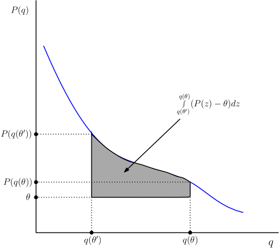
Figure 6: Pictorial depiction of integration along the price axis

Now, suppose $\theta^{\prime}\leq P(q(\theta))$, then (16) implies

$$\int\limits_{q(\theta^{\prime})}^{q(\theta)}(P(z)-\theta)dz \geq\int\limits_{\theta}^{\theta^{\prime}}(q(\theta)-q(\theta^{\prime}))d\tilde{\theta}\geq\int\limits_{\theta}^{\theta^{\prime}}(q(\tilde{\theta})-q(\theta^{\prime}))d\tilde{\theta}$$ (17)

where the second inequality holds because $q$ is decreasing. If $\theta^{\prime}>P(q(\theta))$, we know by DD, $q_{e}(\theta^{\prime})\geq q(\theta^{\prime})$, and hence, $P(q(\theta^{\prime}))\geq P(q_{e}(\theta^{\prime}))=\theta^{\prime}$. This implies that $\theta^{\prime}\in[P(q(\theta)),P(q(\theta^{\prime}))]$. Again, using equation (16), we get

$$\int\limits_{q(\theta^{\prime})}^{q(\theta)}(P(z)-\theta)dz \geq\int\limits_{\theta}^{P(q(\theta))}(q(\theta)-q(\theta^{\prime}))d\tilde{\theta}+\int\limits_{P(q(\theta))}^{\theta^{\prime}}(P^{-1}(\tilde{\theta})-q(\theta^{\prime}))d\tilde{\theta}$$

$$\geq\int\limits_{\theta}^{P(q(\theta))}(q(\theta)-q(\theta^{\prime}))d\tilde{\theta}+\int\limits_{P(q(\theta))}^{\theta^{\prime}}(q(\tilde{\theta})-q(\theta^{\prime}))d\tilde{\theta}$$ (by DD)

$$\geq\int\limits_{\theta}^{P(q(\theta))}(q(\tilde{\theta})-q(\theta^{\prime}))d\tilde{\theta}+\int\limits_{P(q(\theta))}^{\theta^{\prime}}(q(\tilde{\theta})-q(\theta^{\prime}))d\tilde{\theta} q$$ (since is decreasing)

$$=\int\limits_{\theta}^{\theta^{\prime}}(q(\tilde{\theta})-q(\theta^{\prime}))d\tilde{\theta}$$ (18)

By inequalities (17) and (18), we have

$$\int\limits_{q(\theta^{\prime})}^{q(\theta)}(P(z)-\theta)dz \geq\int\limits_{\theta}^{\theta^{\prime}}(q(\tilde{\theta})-q(\theta^{\prime}))d\tilde{\theta}$$

Thus, (15) implies that $\textsc{RS}_{\alpha}(\theta,M)\geq\textsc{RS}_{\alpha}(\theta^{\prime},M)$ with a strict inequality holding for $\alpha\in(0,1)$. $\blacksquare{}$

Proof of Proposition 2. We begin by arguing that it is without loss to focus attention on floor randomized mechanisms satisfying DD and left-continuity. To see why, pick any IC and IR mechanism $M$ that violates either of these properties. By Theorem 2, there exists a floor randomized mechanism satisfying DD and left-continuity, say $M^{\prime}$, that dominates $M$. Moreover,

$$\inf_{G\in\mathcal{G}}\textsc{RS}_{\alpha}(M^{\prime},G)=_{(a)}\textsc{RS}_{\alpha}(M^{\prime},G^{\star}) \geq_{(b)}\textsc{RS}_{\alpha}(M,G^{\star})\geq\inf_{G\in\mathcal{G}}\textsc{RS}_{\alpha}(M,G)$$

where equality $(a)$ holds because of Lemma 3. As for inequality $(b)$, it holds because $M^{\prime}$ dominates $M$. Notice that the set of floor randomized mechanisms satisfying DD and left-continuity is non-empty, and therefore, there exists a max-min optimal mechanism which satisfies these three properties.

To complete the proof, it suffices to argue that $M_{G^{\star}}$, where

$$M_{G^{\star}}\in\arg\max_{M\in\mathcal{N}}~{}\textsc{RS}_{\alpha}(M,G^{\star}),$$ (19)

is indeed max-min optimal in the set $\mathcal{N}$ of floor randomized mechanisms satisfying DD and left-continuity. By Lemma 3, infimum occurs at $G^{\star}$ for all such mechanisms. And because of equation (19), mechanism $M_{G^{\star}}$ attains the maximum regulator’s surplus among all such mechanisms at $G^{\star}$. $\blacksquare{}$

References

- Amador and Bagwell (2022) Amador, M. and K. Bagwell (2022): “Regulating a monopolist with uncertain costs without transfers,” Theoretical Economics, 17, 1719–1760.
- Armstrong (1999) Armstrong, M. (1999): “Optimal regulation with unknown demand and cost functions,” Journal of Economic Theory, 84, 196–215.
- Armstrong and Rochet (1999) Armstrong, M. and J.-C. Rochet (1999): “Multi-dimensional screening: A user’s guide,” European Economic Review, 43, 959–979.
- Armstrong and Sappington (2004) Armstrong, M. and D. E. Sappington (2004): “Toward a synthesis of models of regulatory policy design with limited information,” Journal of Regulatory Economics, 26, 5–21.
- Armstrong and Sappington (2006) ——— (2006): “Regulation, competition and liberalization,” Journal of Economic Literature, 44, 325–366.
- Athanasiou and Valletta (2021) Athanasiou, E. and G. Valletta (2021): “Undominated mechanisms and the provision of a pure public good in two agent economies,” Social Choice and Welfare, 57, 763–795.
- Baron and Myerson (1982) Baron, D. P. and R. B. Myerson (1982): “Regulating a monopolist with unknown costs,” Econometrica, 50, 911–930.
- Bergemann et al. (2023) Bergemann, D., T. Heumann, and S. Morris (2023): “Cost based nonlinear pricing,” Cowles Foundation for Research in Economics, Yale University.
- Borgers et al. (2024) Borgers, T., J. Li, and W. Kexin (2024): “Undominated mechanisms,” Presented at Conference of Mechansms and Institution Design.
- Carroll (2017) Carroll, G. (2017): “Robustness and separation in multidimensional screening,” Econometrica, 85, 453–488.
- Carroll (2019) ——— (2019): “Robustness in mechanism design and contracting,” Annual Review of Economics, 11, 139–166.
- Dana Jr (1993) Dana Jr, J. D. (1993): “The organization and scope of agents: Regulating multiproduct industries,” Journal of Economic Theory, 59, 288–310.
- Guo and Shmaya (2024) Guo, Y. and E. Shmaya (2024): “Robust monopoly regulation,” Working Paper.
- Hart and Reny (2015) Hart, S. and P. J. Reny (2015): “Maximal revenue with multiple goods: Nonmonotonicity and other observations,” Theoretical Economics, 10, 893–922.
- Kazumura et al. (2020) Kazumura, T., D. Mishra, and S. Serizawa (2020): “Strategy-proof multi-object mechanism design: Ex-post revenue maximization with non-quasilinear preferences,” Journal of Economic Theory, 188, 105036.
- Laffont and Tirole (1986) Laffont, J.-J. and J. Tirole (1986): “Using cost observation to regulate firms,” Journal of Political Economy, 94, 614–641.
- Lewis and Sappington (1988a) Lewis, T. R. and D. E. Sappington (1988a): “Regulating a monopolist with unknown demand,” American Economic Review, 986–998.
- Lewis and Sappington (1988b) ——— (1988b): “Regulating a monopolist with unknown demand and cost functions,” The RAND Journal of Economics, 438–457.
- Manelli and Vincent (2007) Manelli, A. M. and D. R. Vincent (2007): “Multidimensional mechanism design: Revenue maximization and the multiple-good monopoly,” Journal of Economic Theory, 137, 153–185.
- Sprumont (2013) Sprumont, Y. (2013): “Constrained-optimal strategy-proof assignment: Beyond the Groves mechanisms,” Journal of Economic Theory, 148, 1102–1121.
- Yang and Zentefis (2023) Yang, K. H. and A. K. Zentefis (2023): “Regulating oligopolistic competition,” Journal of Economic Theory, 212, 105709.